DNS of horizontal open channel flow with finite-size, heavy particles at low solid volume fraction

Abstract

We have performed direct numerical simulation of turbulent open channel flow over a smooth horizontal wall in the presence of finite-size, heavy particles. The spherical particles have a diameter of approximately $7$ wall units, a density of $1.7$ times the fluid density and a solid volume fraction of $5\cdot 10^{-4}$. The value of the Galileo number is set to $16.5$ , while the Shields parameter measures approximately $0.2$. Under these conditions, the particles are predominantly located in the vicinity of the bottom wall, where they exhibit strong preferential concentration which we quantify by means of Voronoi analysis and by computing the particle-conditioned concentration field. As observed in previous studies with similar parameter values, the mean streamwise particle velocity is smaller than that of the fluid. We propose a new definition of the fluid velocity “seen” by finite-size particles based on an average over a spherical surface segment, from which we deduce in the present case that the particles are instantaneously lagging the fluid only by a small amount. The particle-conditioned fluid velocity field shows that the particles preferentially reside in the low-speed streaks, leading to the observed apparent lag. Finally, a vortex eduction study reveals that spanwise particle motion is significantly correlated with the presence of vortices with the corresponding sense of rotation which are located in the immediate vicinity of the near-wall particles.

1 Introduction

The transport of solid particles in wall bounded turbulent flows is a common occurrence in various natural and man-made systems. This transport phenomenon has significant implications in many environmental and industrial processes. For instance one of the key environmental variables in river geomorphology is sediment transport, which involves the erosion, movement and deposition of sediment particles by the fluid flow. An improved understanding of the coupled interaction between solid particles and turbulence is highly desirable as it would pave the way for improvements of engineering-type formulas. However the complex structure of wall-bounded shear flows and the dependence on multiple governing parameters has made this task very challenging to the present date.

Experimental studies of particle-turbulence interaction in horizontal channel flow show that near-wall coherent structures play an important role in the dynamics of particle motion (see e.g. Sumer and Oğuz, 1978; Yung et al., 1989; Rashidi et al., 1990; Kaftori et al., 1995a, b; Niño and García, 1996; Kiger and Pan, 2002; Righetti and Romano, 2004). Rashidi et al. (1990) investigated the coupled interaction between phases in a horizontal channel flow laden with heavy spherical particles. They observed that most of the particles, once they settle to the bottom wall, accumulate in the low-speed streaks. The particles, depending on their size, their density and flow Reynolds number, are observed to get lifted up and entrained into the outer flow presumably by the action of the coherent structures. Particles resettling to the bottom are observed to migrate into the low-speed fluid regions, supposedly by the action of the eddy structures. Hetsroni and Rozenblit (1994) found similar particle segregation at the wall when investigating particles with a diameter of 10 wall units (i.e. equal to 10 times the viscous length scale $\nu/u_{\tau}$ where $\nu$ is the kinematic viscosity of the fluid and $u_{\tau}$ is the friction velocity). However, larger particles having a diameter of more than 30 wall units did not accumulate in the low-speed fluid regions; rather they formed a random distribution at the bottom wall of their horizontal flume. In similar experiments, Kaftori et al. (1995a) and Niño and García (1996) investigated the effect of the coherent structures on particle motion, distribution, entrainment as well as deposition in the wall region. They show that heavy particles directly interact with the flow structures. At the bottom wall, particles were observed to be non-uniformly distributed and to form streamwise aligned streaks. The shape, length and persistence with time of these streaks was observed to vary with the particle size and/or the flow rate. Formation of particle streaks was also observed by Yung et al. (1989) even for particles which are completely submerged within the viscous sublayer (diameter smaller than $1.3$ wall units). The experimental studies of Kaftori et al. (1995b); Kiger and Pan (2002); Righetti and Romano (2004) were focused on the characteristics of suspended heavy particles and their turbulence modulation effects in open as well as closed channel flows. These experiments showed that generally, the mean streamwise velocity of the particles is smaller than that of the fluid except for those particles located in a layer very close to the wall where contrarily particle velocity is reported to be on average higher than that of the fluid.

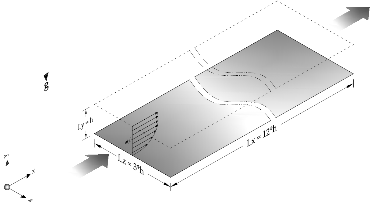
Figure 1: Geometrical configuration of the present simulation. Gravity is directed in the negative y- direction. The computational domain is periodic along the x- and z-directions.

The majority of available numerical studies on particle-turbulence interaction are based on the point-particle approach (see e.g. Rouson and Eaton, 2001; Marchioli and Soldati, 2002; Narayanan et al., 2003; Picciotto et al., 2005). Studies based on this approach show that there is a strong correlation between the near-wall coherent structures and particle deposition and entrainment processes as well as the resulting preferential particle segregation. The degree of the correlation is found to be dependent on the Stokes number, i.e. the ratio of the particle response time to some representative time scale of the flow (Soldati and Marchioli, 2009). However, the point-particle approach is limited to particle sizes which are much smaller than the smallest flow scales. Therefore, in order to numerically investigate finite-size effects, one has to resort to simulations which fully resolve the particles.

Recently more faithful simulations in which the interface between the phases is resolved to accurately compute the flow field at the particle scale are starting to emerge both for wall bounded flows (Pan and Banerjee, 1997; Uhlmann, 2008; Shao et al., 2012; García-Villalba et al., 2012) and unbounded flows (Kajishima and Takiguchi, 2002; Ten Cate et al., 2004; Lucci et al., 2010, 2011). In one of the first simulations of this kind, Pan and Banerjee (1997) simulated horizontal open channel flow seeded with a small number of fixed and moving particles of diameter 8.5 and 17 wall units at an average solid volume fraction of $\mathcal{O}(10^{-4})$. They observed that the presence of particles strongly affected the turbulent structures. Uhlmann (2008) and García-Villalba et al. (2012) simulated vertically oriented channel flow seeded with freely moving heavy particles with a diameter of approximately 11 wall units at a solid volume fraction of $0.4\%$. These simulations revealed that the particles strongly modified the flow and lead to the formation of very large streamwise-elongated flow structures. Recently, Shao et al. (2012) simulated particle-laden turbulent flow in a horizontal channel. They considered heavy particles (with density $1.5$ times that of the fluid) which are relatively large in size (with diameter $10\%$ and $20\%$ of the half channel height), at relatively large solid volume fraction values (up to $7\%$). They reported that, in cases where settling effects are not considered (without gravity), the particle distribution was homogeneous and the mean fluid and particle velocities were equal. However, when settling effects are considered, they reported that most particles settle to the bottom wall where they accumulate in the low-speed fluid regions.

$Re_{\mathrm{b}}$	$Re_{\tau}$	$\rho_{\mathrm{p}}/\rho_{\mathrm{f}}$	$D/h$	$D^{+}$	$St^{+}$	$St_{\mathrm{b}}$	$\Phi_{\mathrm{s}}$	$|\mathbf{g}|h/u_{\mathrm{b}}^{2}$	$Ga$	$\theta$
$2870$	$184.54$	$1.7$	$10/256$	$7.21$	$4.91$	$0.41$	$0.05\%$	$0.80$	$16.49$	$0.19$

Table 1: Physical parameters of the simulation. $Re_{\mathrm{b}}$ is the Reynolds number based on the channel depth $h$ and bulk velocity $u_{\mathrm{b}}$. $Re_{\tau}$ is the Reynolds number based on $h$ and the friction velocity $u_{\tau}$. $St^{+}$ and $St_{\mathrm{b}}$ are the Stokes numbers based on near wall fluid time scale and bulk time scale respectively. $D$ is the diameter of the spherical particles. $\Phi_{\mathrm{s}}$ is the global solid volume fraction and $|\mathbf{g}|$ is the magnitude of acceleration due to gravity. $Ga$ and $\theta$ are the Galileo number and Shields number, respectively.

$L_{\mathrm{x}}\times L_{\mathrm{y}}\times L_{\mathrm{z}}$	$N_{\mathrm{x}}\times N_{\mathrm{y}}\times N_{\mathrm{z}}$	$D/\Delta x$	$\Delta x^{+}$	$N_{\mathrm{p}}$	$T_{\mathrm{obs}}u_{\mathrm{b}}/h$
$12h\times h\times 3h$	$3072\times 257\times 768$	$10$	$0.72$	$518$	$255$

Table 2: Numerical parameters of the simulation. $L_{i}$ and $N_{i}$ are the computational domain length and number of grid points employed in the $i$th coordinate direction, respectively. $N_{\mathrm{p}}$ is the number of particles considered. $T_{\mathrm{obs}}$ is the observation time of the simulations excluding the transient period.

The general picture that has emerged from previous studies of horizontal turbulent channel flow with heavy particles (in the regime where streaky particle patterns are observed) can be summed up briefly as follows. Sweeps of high-speed fluid as well as gravitational settling bring suspended heavy particles towards the wall. Through the action of the quasi-streamwise vortices, particles near the wall are forced to move in the spanwise direction into the low-speed regions, resulting in particle accumulation in the form of persistent streaky particle patterns. The counter-rotating quasi-streamwise vortices flanking the low-speed streaks generate ejections of low-momentum fluid away from the wall. These ejection events are the predominant sources of upward particle motion from the wall. Concerning the difference between the mean fluid velocity and the mean particle velocity (i.e. particles apparently lagging the fluid), it is believed to be a statistical consequence of particles preferentially residing in the low-speed regions, rather than a manifestation of particles instantaneously lagging the surrounding fluid in a significant manner.

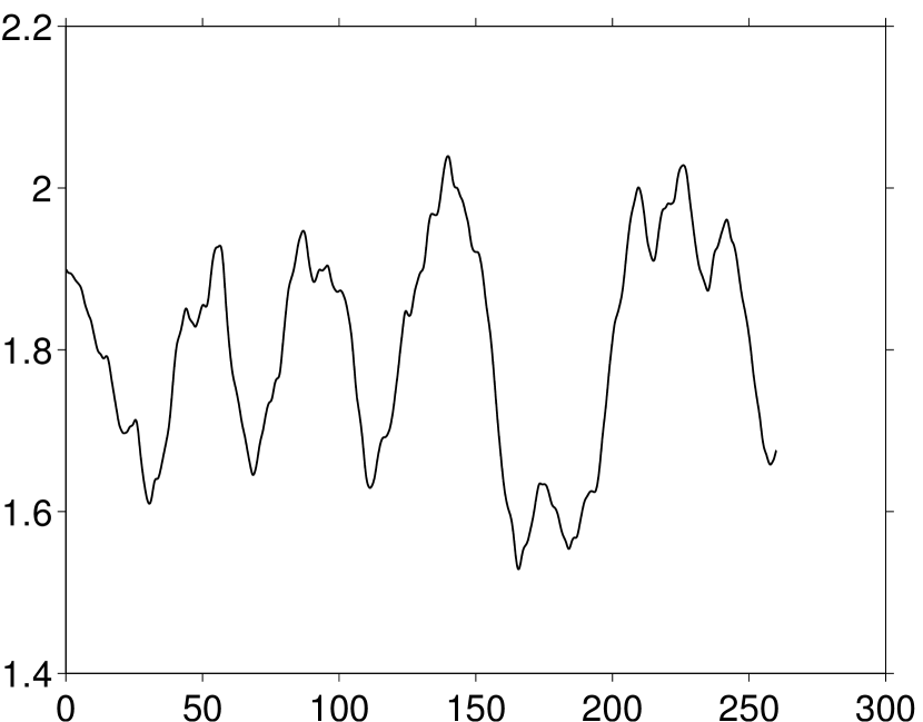
$(a)$

$t/T_{\mathrm{b}}$

$\langle k\rangle_{\mathrm{xyz}}/u_{\tau}^{2}$

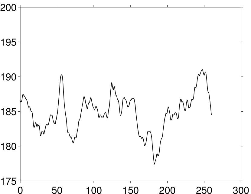
$(b)$

$t/T_{\mathrm{b}}$

$Re_{\tau}$

Figure 2: Time evolution of (a) box-averaged turbulent kinetic energy and (b) friction-velocity based Reynolds number. Note that the time coordinate has been shifted to the beginning of the observation interval, excluding initial transients.

Despite the great progress achieved through past studies, a number of important questions still remain unanswered. The present work is an attempt to fill these gaps. First, a detailed characterization of the spatial structure of the dispersed phase in horizontal channel flow with finite-size particles is still lacking. For this purpose an analysis based upon Voronoi tesselation relative to the instantaneous particle distribution is an adequate instrument, as has been demonstrated by Monchaux, Bourgoin, and Cartellier (2010) and Monchaux, Bourgoin, and Cartellier (2012). Additionally, the particle-pair distribution function yields complementary information on the large-scale structure of the particle ‘field’. Second, in order to rigorously confirm the explanation of the apparent velocity lag of the particles in terms of preferential sampling of the fluid velocity field, the possibility of a systematic instantaneous inter-phase velocity lag needs to be excluded. This in turn requires the definition of a characteristic fluid velocity in the vicinity of the particles (often referred to as the velocity ‘seen’ by the particles). However, for finite-size particles a unique definition does not exist, and for different reasons previous attempts (Bagchi and Balachandar, 2003; Merle et al., 2005; Zeng et al., 2008; Lucci et al., 2010) do not yield the desired results in the present flow configuration. Here we propose a new definition of the fluid velocity seen by finite-size particles. A third point of interest concerns the fluid velocity field conditioned upon the presence of particles and, in particular, the relation between the spanwise motion of near-wall particles (driving particles into low-speed streaks) and the presence of coherent vortices.

In order to investigate these three aspects of the problem, highly-resolved flow and particle data (in time and space) is required. In the present work we have generated such data by means of interface-resolved direct numerical simulation of particle-laden, horizontal, open channel flow over a smooth wall. All relevant scales of the flow problem are resolved by means of a finite-difference/immersed-boundary technique. The solid volume fraction was set to a relatively low value in order to avoid a dominance of inter-particle collisions. Contact between pairs of particles and contact of particles with the solid wall is considered as frictionless in the simulations.

$(a)$

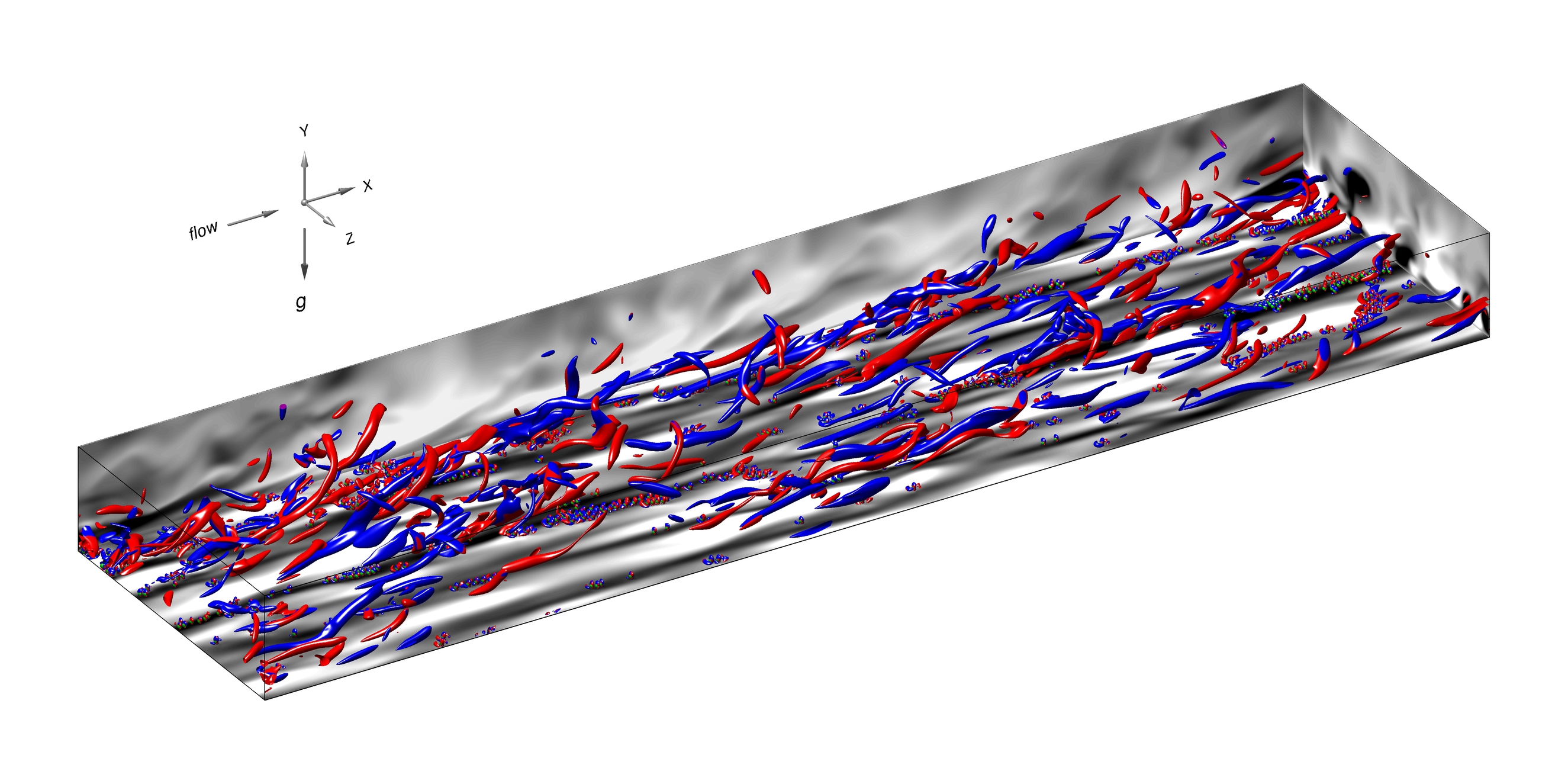
$3h$                                                                   $12h$

$h$

$(b)$

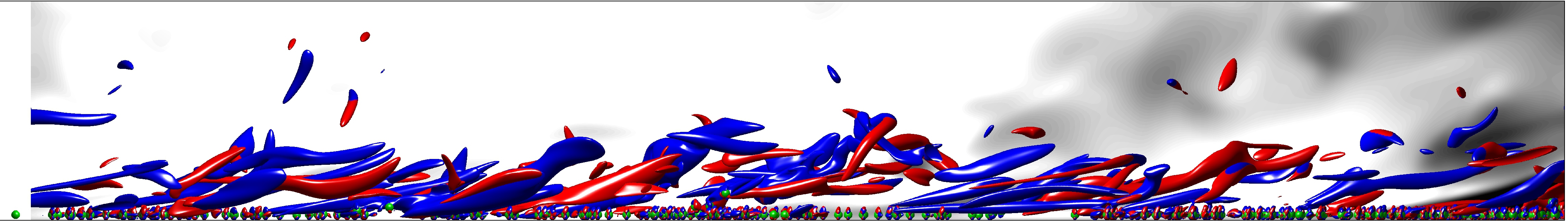
Figure 3: Instantaneous three-dimensional snapshot of the flow field and the particle positions (observed mostly residing at the bottom wall). Strong vortical regions are shown by plotting a negative-valued iso-surface of the $\lambda_{2}$ field (cf. definition in § 3.6). The iso-surfaces are colored (red/blue) based on the sign of the streamwise vorticity (positive/negative). The greyscales indicate values of the streamwise velocity fluctuation in a wall-parallel plane at $y^{+}=5$ (projected upon the plane $y=0$ for better visibility) and in wall perpendicular planes at $x/h=12$ and $z/h=0$, ranging from black (minimum negative values) to white (maximum positive values). Note that although the particle surfaces are colored in green, particles appear mostly in either red or blue color, due to vortical structures located in their immediate vicinity. A close-up of the same graph looking against the spanwise direction is shown in $(b)$ (i.e. the flow is from left to right).

2 Computational methodology and setup

2.1 Numerical method

The numerical method employed in the present study is a formulation of the immersed boundary method for the simulation of particulate flows developed by Uhlmann (2005a). The basic idea of the immersed boundary method is to solve the modified incompressible Navier-Stokes equations throughout the entire domain $\Omega$ comprising the fluid domain $\Omega_{\mathrm{f}}$ and the domain occupied by the suspended particles $\Omega_{\mathrm{s}}$ while adding a force term which serves to impose the no-slip condition at the fluid-solid interface. The immersed boundary technique is realized in the framework of a standard fractional step method for the incompressible Navier-Stokes equations. The temporal discretization is semi-implicit, based on the Crank-Nicolson scheme for the viscous terms and a low-storage three-step Runge-Kutta procedure for the non-linear part (Verzicco and Orlandi, 1996). The spatial operators are evaluated by central finite-differences on a staggered grid. The temporal and spatial accuracy of this scheme are of second order. In the computation of the forcing term, the necessary interpolation of variable values from Eulerian grid positions to particle-related Lagrangian positions (and the inverse operation of spreading the computed force terms back to the Eulerian grid) are performed by means of the regularized delta function approach of Peskin (2002). This procedure yields a smooth temporal variation of the hydrodynamic forces acting on individual particles while they are in arbitrary motion with respect to the fixed grid. The employed Cartesian grid is uniform and isotropic in order to ensure the conservation of important quantities such as the total force and torque, during the interpolation and spreading procedure. The particle motion is determined by the Runge-Kutta-discretized Newton equations for linear and angular motion of rigid bodies, driven by buoyancy, hydrodynamic forces/torque and contact forces (in case of collisions).

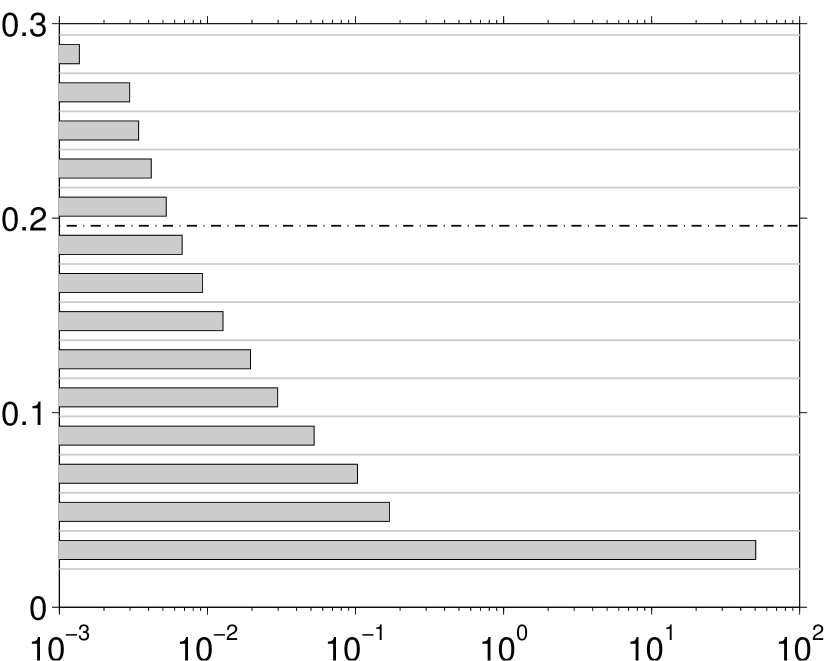
$\langle\phi_{s}\rangle/\Phi_{s}$

$\quad y/h$

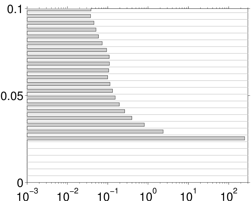
Figure 4: Profile of the average solid volume fraction $\langle\phi_{s}\rangle$, normalized by the global value $\Phi_{s}$. The width of the averaging bins are shown with gray-colored lines. The number of data samples located in bins above the chain-dotted line (at $y^{+}=36$) is smaller than 800. Note that the bin adjacent to the wall has zero number of samples as there is no particle center in the interval $0\leq y_{\mathrm{p}}<D/2$. The insert shows the same quantity for an interval close to the wall, evaluated with finer averaging bins $\Delta h=\Delta x$.

During the course of a simulation, particles can closely approach each other. However, very thin inter-particle fluid films cannot be resolved by a typical grid, and therefore, the correct buildup of repulsive pressure is not captured, which, in turn, can lead to possible partial “overlap” of the particle positions in the numerical computation. In practice, particle-particle contacts are treated by a simple repulsive force mechanism (Glowinski et al., 1999), which is active for particle pairs at a distance smaller than two grid spacings. The contact force only acts in the normal direction (along the line connecting the two particles’ centers) and frictional contact forces are not considered. The analogous treatment is applied to particle-wall contact. Note that a posteriori evaluation of the particle trajectories revealed that the average temporal interval between two collision events measures approximately $4.1$ bulk flow time units.

The numerical method employs domain decomposition for parallelism and has been shown to run on grids of up to $8192^{3}$, using up to ${\cal O}(10^{5})$ processor cores in scaling tests (Uhlmann, 2010). The numerical method has been validated on a whole range of benchmark problems (Uhlmann, 2004, 2005a, 2005b, 2006), and has been previously employed for the simulation of several flow configurations (Uhlmann, 2008; Chan-Braun et al., 2011; García-Villalba et al., 2012).

2.2 Flow configuration and parameter values

Horizontal open channel flow laden with finite-size, heavy, spherical particles is considered including the action of gravity. As shown in figure 1, a Cartesian coordinate system is adopted such that $x$, $y$, and $z$ are the streamwise, wall-normal and spanwise directions respectively. Mean flow and gravity are directed in the positive $x$ and the negative $y$ directions respectively. The computational domain is periodic in the homogeneous directions (streamwise and spanwise).

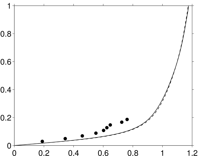
$(a)$

$\langle u_{\mathrm{f}}\rangle/u_{\mathrm{b}},\langle u_{\mathrm{p}}\rangle/u_{\mathrm{b}}$

$\quad y/h$

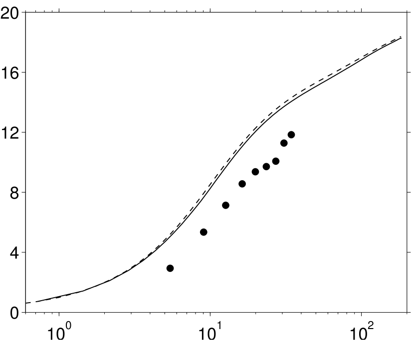
$(b)$

$y^{+}$

$\langle u_{\mathrm{f}}\rangle/u_{\tau},\langle u_{\mathrm{p}}\rangle/u_{\tau}$

Figure 5: Wall-normal profile of the mean streamwise fluid velocity (solid line) and particle velocity (filled symbols) both in (a) outer units and (b) wall units. The dashed line represents the corresponding profile of a single phase flow at a bulk Reynolds number identical to the current simulation.

A free-slip condition is imposed at the top boundary while the no-slip condition is imposed at the bottom wall. The channel is driven by a horizontal mean pressure gradient imposing a constant flow rate. The Reynolds number of the flow based on the channel height $h$ and the bulk velocity $u_{\mathrm{b}}~{}\equiv~{}\frac{1}{h}\int_{0}^{h}\langle u_{\mathrm{f}}\rangle\mathrm{d}y$ is set to a value $Re_{\mathrm{b}}\equiv u_{\mathrm{b}}h/\nu=2870$ generating a turbulent flow at a friction Reynolds number $Re_{\tau}\equiv u_{\tau}h/\nu=184$, where $u_{\tau}\equiv\sqrt{\langle\tau_{\mathrm{w}}\rangle/\rho}$ is the friction velocity, and $\langle\tau_{\mathrm{w}}\rangle$ is the mean shear stress averaged in time and over the solid wall at $y=0$. The value of the friction velocity matches the value obtained in single-phase flow at the same bulk Reynolds number to within $1\%$. The spherical particles considered are relatively small in size when compared to the channel depth (particle diameter $D/h=10/256$) but they are larger than the viscous length scale ($D^{+}=7.21$). Note that the “⁺” superscript indicates scaling in wall units. The particle-to-fluid density ratio is set to a value of $\rho_{\mathrm{p}}/\rho_{\mathrm{f}}=1.7$. The Stokes number is defined as the ratio between the particle relaxation time scale $\tau_{\mathrm{p}}\equiv\rho_{\mathrm{p}}/\rho_{\mathrm{f}}D^{2}/(18\nu)$, assuming Stokes drag law, and a fluid time scale. The Stokes number based on the near wall fluid time scale has a value $St^{+}\equiv\tau_{\mathrm{p}}u_{\tau}^{2}/\nu=4.9$ and the Stokes number based on bulk fluid time scale $T_{\mathrm{b}}\equiv h/u_{\mathrm{b}}$ has a value of $St_{\mathrm{b}}\equiv\tau_{\mathrm{p}}/T_{\mathrm{b}}=0.41$. The global solid volume fraction was set to $\Phi_{\mathrm{s}}=5\times 10^{-4}$. This means that there are $N_{\mathrm{p}}=518$ particles in the computational domain $\Omega$ of size $12h\times h\times 3h$. The non-dimensional gravity constant $gh/u_{\mathrm{b}}^{2}$ was set to a value $0.8$ such that the Galileo number, defined as $Ga^{2}=(\rho_{\mathrm{p}}/\rho_{\mathrm{f}}-1)gD^{3}/\nu^{2}$ has a value $Ga=16.49$ and the Shields number, defined as $\theta^{-1}=(\rho_{\mathrm{p}}/\rho_{\mathrm{f}}-1)gD/u_{\tau}^{2}$ has a value $\theta=0.19$. The computational domain is discretized by a uniform isotropic grid with grid spacing $\Delta x=\Delta y=\Delta z=h/256$. This grid spacing yields a particle resolution of $D/\Delta x=10$ and in terms of wall units $\Delta x^{+}\approx 0.7$. Table 1 and table 2 summarize the important physical and numerical parameter values adopted.

The simulation was first initiated on a coarser grid (by a factor of two in each coordinate direction), using a fully turbulent flow field with particles distributed throughout the computational domain as initial condition. A transient of roughly $40\,T_{\mathrm{b}}$ was observed, after which the particles had formed patterns very similar to those observed and described below. Then the final data of the coarser-grid simulation was interpolated upon the current grid, and the simulation was continued for another $252\,T_{\mathrm{b}}$. The entire initial interval of $560\,T_{\mathrm{b}}$ was unintentionally computed with an incorrect value of the particles’ moment of inertia ($\rho_{p}D^{5}\pi 5/48$ instead of $\rho_{p}D^{5}\pi/60$). After correcting the value of the moment of inertia, the simulation was run for additional $260\,T_{\mathrm{b}}$, the first $5\,T_{\mathrm{b}}$ of which have been discarded. Therefore, the temporal observation interval over which the present data was generated measures $T_{\mathrm{obs}}=255\,T_{b}$.

Figure 2 shows the time evolution over the observation interval of the box-averaged turbulent kinetic energy, defined as $\langle k\rangle_{\mathrm{xyz}}=\frac{1}{2}(\langle u_{\mathrm{f},i}u_{\mathrm{f},i}\rangle_{\mathrm{xyz}}-\langle u_{\mathrm{f},i}\rangle_{\mathrm{xyz}}\langle u_{\mathrm{f},i}\rangle_{\mathrm{xyz}})$, where $\langle\cdot\rangle_{\mathrm{xyz}}$ denotes an instantaneous average over the domain occupied by the fluid, as defined in (22). The time evolution of $Re_{\tau}$ based upon the instantaneous value of the friction velocity is also presented in the figure. Several cycles of large-scale fluctuations can be observed. The reader is referred to A for a statistical convergence check based on the balance of the mean streamwise momentum.

Figure 3 gives an impression of the size of the domain, the coherent flow structures and the particle distribution.

The simulation was typically performed on $48$ to $256$ processor cores and required roughly half a million core hours of CPU time.

In addition, we have generated single-phase reference data at the same parameter point by means of a pseudo-spectral method (Kim et al., 1987). This reference simulation has been run for over $4400$ bulk time units, i.e. a considerably longer interval than that of the main simulation. The single-phase data will be used for the purpose of comparison in the following.

2.3 Notation

Before turning to the results, let us fix the basic notation followed throughout the present text. Velocity vectors and their components corresponding to the fluid and the particle phases are distinguished by subscript “f” and “p”, respectively, as in $\mathbf{u}_{\mathrm{f}}=(u_{\mathrm{f}},v_{\mathrm{f}},w_{\mathrm{f}})^{T}$ and $\mathbf{u}_{\mathrm{p}}=(u_{\mathrm{p}},v_{\mathrm{p}},w_{\mathrm{p}})^{T}$. Similarly, the particle position vector is denoted as $\mathbf{x}_{\mathrm{p}}=(x_{\mathrm{p}},y_{\mathrm{p}},z_{\mathrm{p}})^{T}$ and the vector of angular particle velocity as $\boldsymbol{\omega}_{\mathrm{p}}=(\omega_{\mathrm{p,x}},\omega_{\mathrm{p,y}},\omega_{\mathrm{p,z}})^{T}$.

Fluctuations of the fluid velocity field with respect to the average over wall-parallel planes and time are henceforth denoted by a single prime, i.e. $\mathbf{u}_{\mathrm{f}}^{\prime}(\mathbf{x},t)=\mathbf{u}_{\mathrm{f}}(\mathbf{x},t)-\langle\mathbf{u}_{\mathrm{f}}\rangle(y)$. Likewise, the fluctuations of the particle velocity are defined as the difference between the instantaneous value and the average (over time and all particles located in predefined wall-normal intervals) at the corresponding location, viz. $\mathbf{u}_{\mathrm{p}}^{\prime}(\mathbf{x}_{\mathrm{p}}(t),t)=\mathbf{u}_{\mathrm{p}}(\mathbf{x}_{\mathrm{p}}(t),t)-\langle\mathbf{u}_{\mathrm{p}}\rangle(y_{\mathrm{p}}(t))$. The reader is referred to B for definitions of the various averaging operators used in the present study.

The particle radius is henceforth denoted as $R=D/2$.

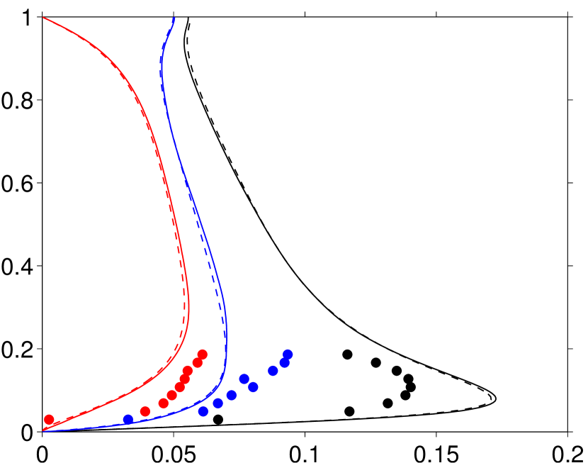
$(a)$

$\langle u^{\prime}_{\mathrm{f},\alpha}u^{\prime}_{\mathrm{f},\alpha}\rangle^{\frac{1}{2}}/u_{\mathrm{b}}$, $\langle u^{\prime}_{\mathrm{p},\alpha}u^{\prime}_{\mathrm{p},\alpha}\rangle^{\frac{1}{2}}/u_{\mathrm{b}}$

$\quad y/h$

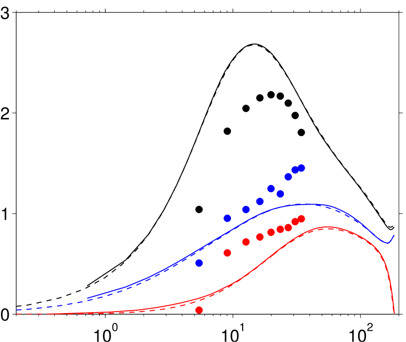
$(b)$

$y^{+}$

$\langle u^{\prime}_{\mathrm{f},\alpha}u^{\prime}_{\mathrm{f},\alpha}\rangle^{\frac{1}{2}}/u_{\tau}$, $\langle u^{\prime}_{\mathrm{p},\alpha}u^{\prime}_{\mathrm{p},\alpha}\rangle^{\frac{1}{2}}/u_{\tau}$

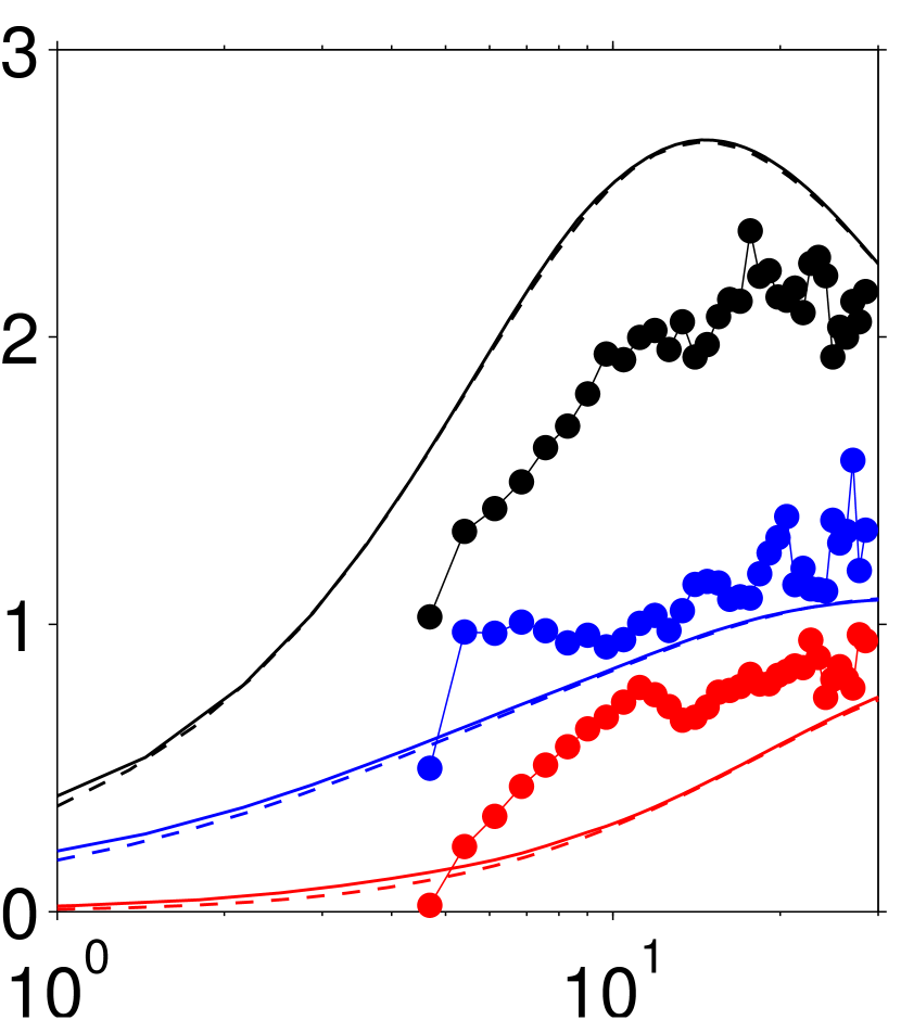
Figure 6: Wall-normal profile of the rms velocity fluctuations of the fluid phase (lines) and particles (filled symbols) in (a) outer units and (b) wall units. The dashed line indicates the single phase data. The black, blue and red colors represent the streamwise, spanwise and wall-normal components of the fluctuations, respectively. The insert shows the same quantities but the particle data is evaluated at finer bins of width $\Delta h=\Delta x$.

3 Results

3.1 Eulerian statistics

3.1.1 Mean solid volume fraction

The global solid volume fraction has such a low value that even if all particles are in contact with the solid wall, their projected area covers less than two percent of the wall-plane, i.e. $N_{p}\pi R^{2}/(L_{x}L_{z})=0.0172$. Figure 4 shows the wall-normal profile of the average solid volume fraction $\langle\phi_{s}\rangle$ (cf. averaging operator defined in equation 25 in B.3). Due to the gravitational settling effect, a strong wall-normal particle concentration gradient forms near the wall. The wall-normal location of the particle centers of the overwhelming majority of all particles ($99.15\%$) is in the interval $D/2\leq y_{\mathrm{p}}<D$ (i.e. corresponding to the second averaging bin). At larger wall-distances, the number of particle samples becomes scarce for the given temporal observation interval. In order to ensure an adequate quality of the statistics, we have chosen to consider only those bins with $y_{\mathrm{p}}^{+}\leq 36$ (up to the dashed line in figure 4), for which the number of samples per bin ranges from a maximum of $10^{7}$ down to $1386$. Therefore, in the following presentation, all Eulerian particle statistics are only provided for wall distances $y^{+}\leq 36$.

3.1.2 Mean streamwise velocity

The profiles of the mean streamwise velocity of fluid and solid phase are shown in figure 5 in outer and inner scaling. Additionally, the data for single-phase flow is included for comparison. In both scalings, the velocity profile of the fluid phase, $\langle u_{\mathrm{f}}\rangle$, almost coincides with the results of the single phase flow. The difference between the curves is smaller than $9.3\times 10^{-3}$ times the maximum velocity, and, therefore, within the range of statistical uncertainty. Thus, for the given parameters, the presence of particles has a negligible effect on the mean fluid velocity profile.

The mean streamwise particle velocity, $\langle u_{\mathrm{p}}\rangle$, is observed to be systematically smaller than that of the fluid phase $\langle u_{\mathrm{f}}\rangle$. The difference in the mean velocities of the two phases, i.e. the apparent velocity lag, is denoted as

$$u_{\mathrm{lag}}=\langle u_{\mathrm{f}}\rangle-\langle u_{\mathrm{p}}\rangle\,,$$ (1)

which is found to vary in the range of $2.1u_{\tau}$ to $3.2u_{\tau}$, corresponding to $0.14u_{\mathrm{b}}$ to $0.21u_{\mathrm{b}}$ (cf. figure 14$b$ which will be discussed below).

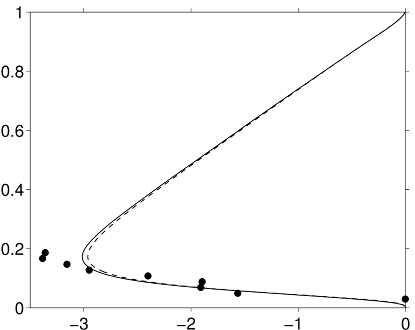
$(a)$

$[\langle u^{\prime}_{\mathrm{f}}v^{\prime}_{\mathrm{f}}\rangle/u^{2}_{\mathrm{b}}$, $\langle u^{\prime}_{\mathrm{p}}v^{\prime}_{\mathrm{p}}\rangle/u^{2}_{\mathrm{b}}]\times 10^{3}$

$\quad y/h$

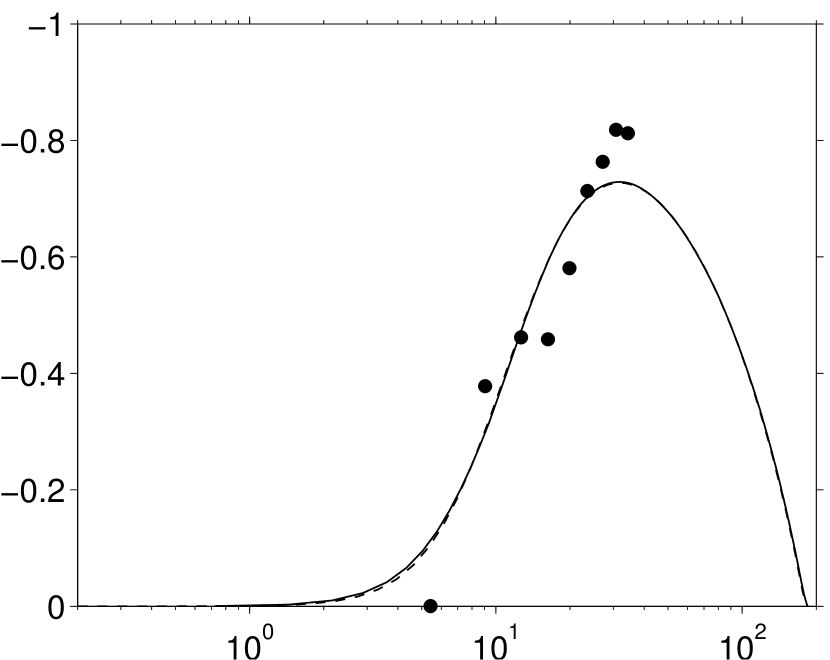
$(b)$

$y^{+}$

$\langle u^{\prime}_{\mathrm{f}}v^{\prime}_{\mathrm{f}}\rangle/u^{2}_{\tau}$, $\langle u^{\prime}_{\mathrm{p}}v^{\prime}_{\mathrm{p}}\rangle/u^{2}_{\tau}$

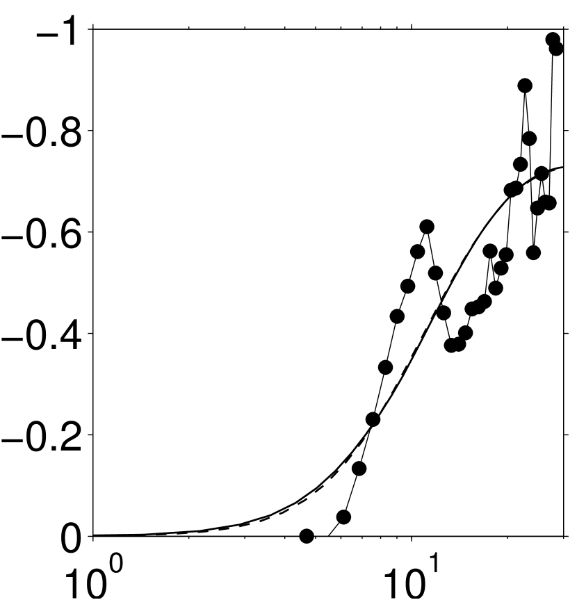
Figure 7: Wall-normal profile of the Reynolds shear stress of the fluid phase (lines) and correlation between streamwise and wall-normal velocity fluctuations of particles (filled symbols) in (a) outer units and (b) wall units. The dashed line indicates the single phase Reynolds stress profiles. The insert shows the same quantities but the particle data is evaluated at finer bins of width $\Delta h=\Delta x$.

The general feature of a positive apparent velocity lag $u_{\mathrm{lag}}>0$ has been reported in a number of experimental studies on horizontal wall-bounded shear flow (Rashidi et al., 1990; Kaftori et al., 1995b; Taniere et al., 1997; Kiger and Pan, 2002; Righetti and Romano, 2004; Muste et al., 2009; Noguchi and Nezu, 2009) as well as in the interface-resolved DNS of horizontal plane channel flow by Shao et al. (2012). The aforementioned references cover a relatively broad range of parameter values in terms of Stokes number, Galileo number and solid volume fraction. Therefore, the phenomenon, which is commonly linked to particles residing preferentially in low-speed regions of the flow, appears to be a relatively ‘robust’ feature of particulate flow in horizontal, wall-bounded, shear turbulence.

However, it should be mentioned that in most of the aforementioned experimental studies a change of sign of the apparent velocity lag is observed – contrary to the present simulations and contrary to those by Shao et al. (2012). Kaftori et al. (1995b) measured particle velocities exceeding the average fluid velocity in a small interval ($y\lesssim D$) very near the wall. The authors, however, attribute this result to measurement errors (influence of the angular particle velocity) rather than to a physical effect. Kiger and Pan (2002) observed average particle velocities leading the average fluid velocity at wall-distances $y^{+}\lesssim 35$; however, they did not further comment on the possible cause for this result. Righetti and Romano (2004) also detected a change of sign of the apparent slip velocity, i.e. $\langle u_{\mathrm{p}}\rangle$ being larger than $\langle u_{\mathrm{f}}\rangle$ for $y^{+}\lesssim 20$ (slightly depending on particle diameter), and vice versa further away from the wall. The authors explained the leading particle velocity near the wall as a consequence of sweep events (i.e. in the fourth quadrant of the $u_{\mathrm{p}}^{\prime},v_{\mathrm{p}}^{\prime}$-plane) dominating the particle transport from the outer flow towards the wall. In the present case, on the contrary, the vast majority of the particles are residing in the direct vicinity of the wall (cf. concentration profile in figure 4), and excursions of individual particles to larger wall-distances occur only very infrequently. Therefore, the importance of particles carrying high streamwise momentum while being swept towards the wall is of little importance to the mean streamwise velocity budget in the region near the wall. As a consequence, negative values of $u_{\mathrm{lag}}$ are not observed in the present case.

In § 3.2 we will return to the apparent velocity lag in order to determine the contribution from the instantaneous lag with respect to a characteristic fluid velocity in the vicinity of the particles. In § 3.4 it will be shown that indeed the decisive contribution stems from particles preferentially sampling the low-speed regions of the flow.

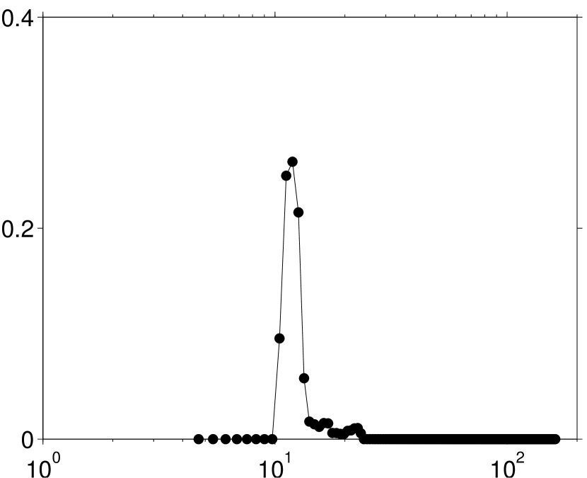
$y^{+}$

$n_{\mathrm{coll}}/n_{\mathrm{p}}^{(j)}$

Figure 8: Wall-normal profile of the number of collision events happening mainly in the vertical direction, i.e. the orientation of the line joining the centers of the two colliding particles is closer to a vertical line than it is to a horizontal line. The collision event is attributed to the particle which is at a larger wall-normal distance than its partner. Data points correspond to the same fine bins adopted in the insert of figure 7.

3.1.3 Covariances of fluid and particle velocity fluctuations

Figure 6 and figure 7 show the wall-normal profiles of the rms velocity fluctuation components of the fluid phase $\langle u^{\prime}_{\mathrm{f},\alpha}u^{\prime}_{\mathrm{f},\alpha}\rangle^{\frac{1}{2}}$ and of the particle phase $\langle u^{\prime}_{\mathrm{p},\alpha}u^{\prime}_{\mathrm{p},\alpha}\rangle^{\frac{1}{2}}$, the Reynolds shear stress profile of the fluid phase $\langle u^{\prime}_{\mathrm{f}}v^{\prime}_{\mathrm{f}}\rangle$ as well as the correlation between the streamwise and wall-normal particle velocity fluctuations $\langle u^{\prime}_{\mathrm{p}}v^{\prime}_{\mathrm{p}}\rangle$. All components of the fluid velocity fluctuation covariances deviate only marginally from the single phase counterparts when normalized both in outer and wall scales. This confirms that the presence of the particles, at the presently adopted parameter values, has a negligible influence on the one-point statistics of the fluid velocity field.

Concerning the dispersed phase, in the near wall region within $y^{+}<36$, the particle velocity fluctuation intensity is observed to be less than that of the fluid fluctuation in the streamwise direction. The reverse is true for the cross-stream components, i.e. in the wall-normal and spanwise directions particle velocity components are observed to fluctuate more strongly than fluid velocities. An exception are those particles which are in the near proximity of the wall (with their centers located at wall normal distance within one particle diameter from the wall) where $\langle v_{\mathrm{p}}^{\prime 2}\rangle$ ($\langle w_{\mathrm{p}}^{\prime 2}\rangle$), is also smaller than $\langle v_{\mathrm{f}}^{\prime 2}\rangle$ ($\langle w_{\mathrm{f}}^{\prime 2}\rangle$). Note that the apparent ‘jump’ from the first to the second data point in figure 6$(b)$ is due to the width of the bins, as can be seen from the insert where much finer sampling bins where used and smoother curves are obtained adjacent to the wall. The insert also demonstrates the limited amount of particle statistics for locations $y^{+}>20$. The overall trend of more isotropic particle velocity fluctuations as compared to the fluid phase can be explained by the action of particle collisions which tend to re-distribute the kinetic energy among the components. Furthermore, as already noted by Kaftori et al. (1995b), the action of gravity in the negative wall-normal direction leads to an additional enhancement of the fluctuation intensity of the wall-normal particle velocity component. On the other hand, the profiles in figure 6$(b)$ (particularly the insert) demonstrate the effect of the finite size of the particles: the damping of the particle velocity fluctuations very close to the wall is felt at larger distances than what is experienced by the fluid, and the wall-normal component has a nearly vanishing fluctuation intensity at center locations around $y^{+}=5$.

Let us turn to the covariance between streamwise and wall-normal velocity fluctuations. Figure 7$(a)$ shows that the fluid and the particle phase exhibit similar values in the near-wall region $y/h\leq 0.2$. Upon closer inspection (figure 7$b$ and insert) it can be seen that the particle ‘Reynolds stress’ tends towards zero at the wall faster than the fluid counterpart, and a cross-over is observed at $y^{+}\approx 7$, which again manifests the finite-size of the particles. However, we detect a clear local maximum of $\langle u^{\prime}_{\mathrm{p}}v^{\prime}_{\mathrm{p}}\rangle$ at a wall-distance of $y^{+}\approx 10$. The insert shows that the particle ‘Reynolds stress’ first decreases significantly for $y^{+}>10$, then rises again for $y^{+}>15$. Although the fluctuation intensity of the two components ($\langle u_{\mathrm{p}}^{\prime}u_{\mathrm{p}}^{\prime}\rangle$ and $\langle v_{\mathrm{p}}^{\prime}v_{\mathrm{p}}^{\prime}\rangle$) does not change much in the interval $10\leq y^{+}\leq 20$, their covariance does exhibit the observed ‘kink’. This means that the correlation between the two components is somehow disturbed in that region. Therefore, we have more carefully investigated the particle paths in the corresponding region. It turns out that particle-particle contact is responsible for the observed behavior. Figure 8 shows the number of detected collisions as a function of wall-distance. In computing the counter, only those collisions were considered which take place in a predominantly vertical direction (i.e. where the line connecting the centers of the two colliding particles is closer to the vertical than to any horizontal axis). By this choice we eliminate those collisions which occur between particles in motion predominantly in a wall-parallel plane. As can be seen, these collisions are concentrated in the same interval of wall-normal distances as the reduction of particle ‘Reynolds stress’ observed in figure 7$(b)$. We have analyzed the trajectories of all particles colliding in the mentioned region (figure omitted), and found that these collisions mostly correspond to either: (i) particles being picked up from the wall by high-speed fluid, then colliding at oblique angles with those particles being located on their downstream side; (ii) particles approaching the near-wall region from the outer flow, then colliding with near-wall particles. In the former case, an ejection (i.e. in the second quadrant of the $u_{\mathrm{p}}^{\prime},v_{\mathrm{p}}^{\prime}$-plane) will be reduced in intensity or converted into a third quadrant event. In the latter case, the collision will tend to convert what is most probably a ‘sweep’ event (fourth quadrant) into a first quadrant event. In both cases, the consequence will be a reduction in amplitude of the (overall negative) correlation between $u_{\mathrm{p}}^{\prime}$ and $v_{\mathrm{p}}^{\prime}$.

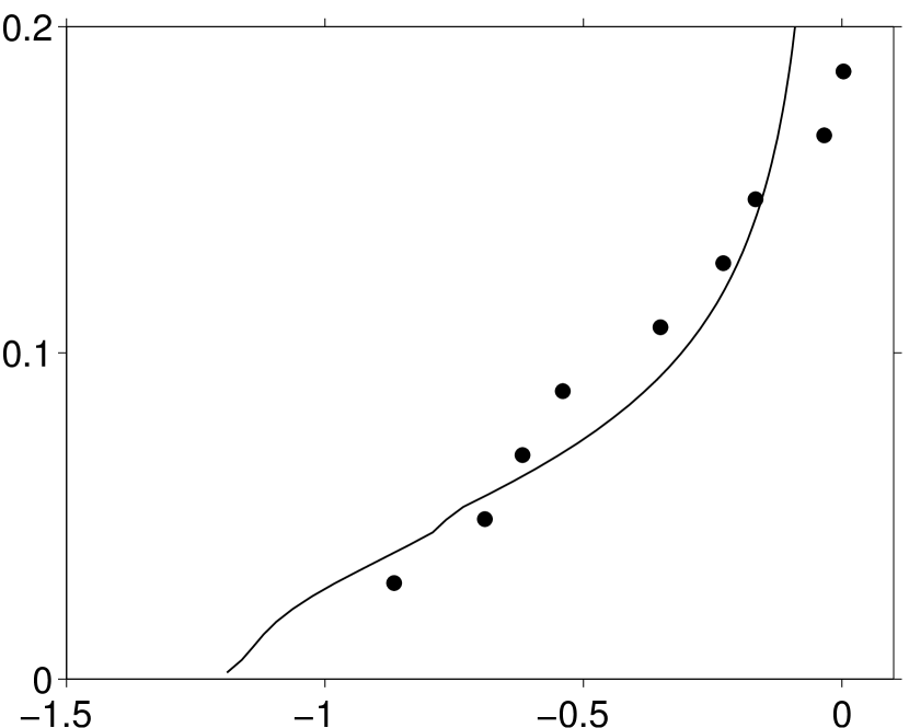
[$-A\,\mathrm{d}\langle u_{\mathrm{f}}\rangle/\mathrm{d}y$; $\langle\omega_{\mathrm{p,z}}\rangle$]$R/u_{\tau}$

$\quad y/h$

Figure 9: Wall-normal profiles of the mean fluid shear (solid line) and mean value of the spanwise component of particle angular velocity (symbols). The proportionality factor is given as $A=0.33.$

3.1.4 Mean shear of the fluid phase and mean angular velocity of the particle phase

Figure 9 shows the profiles of the mean fluid shear, $\mathrm{d}\langle u_{\mathrm{f}}\rangle/\mathrm{d}y$, and the mean angular particle velocity around the spanwise axis, $\langle\omega_{\mathrm{p,z}}\rangle$. The figure suggests that the average particle rotation is driven by the mean shear, as the data points are approximately proportional to the mean fluid velocity gradient. We observe that $\langle\omega_{\mathrm{p,z}}\rangle\approx-A\mathrm{d}\langle u_{\mathrm{f}}\rangle/\mathrm{d}y$ with a proportionality factor of $A\approx 0.33$ (visual fit). An analogous result has already been observed in particulate flow through a vertical channel (Uhlmann, 2008; García-Villalba et al., 2012) where a proportionality factor of $A\approx 0.15$ was obtained. Note that the sign of the angular particle velocity corresponds to forward “rolling” motion. Incidentally, the angular velocity of particles adjacent to the wall is significantly smaller than would be required by a condition of traction on the wall for which $-\langle\omega_{\mathrm{p,z}}\rangle R/\langle u_{\mathrm{p}}\rangle=1$. In the present simulation, the observed value of $-\langle\omega_{\mathrm{p,z}}\rangle R/\langle u_{\mathrm{p}}\rangle$ in the averaging bin adjacent to the wall is equal to $0.3$. Please note that there is no need for particles to actually obey a traction condition in the present setup even if they remain in contact with the wall, since tangential forces were neglected in our contact model.

$(a)$

$z/h$

$(u_{\mathrm{f}}-\langle u_{\mathrm{f}}\rangle)/u_{\tau}$

$(b)$

$z/h$

$(u_{\mathrm{f}}-\langle u_{\mathrm{f}}\rangle)/u_{\tau}$

$(c)$

$z/h$

$\varepsilon^{+}$

$(d)$

$z/h$

$x/h$

$\varepsilon^{+}$

Figure 10: Visualization of instantaneous flow fields in a wall-parallel plane located at $y^{+}=5$. Graphs $(a)$ and $(b)$ show fluctuations of the streamwise fluid velocity component, $(c)$ and $(d)$ show the instantaneous dissipation rate of fluctuating kinetic energy, $\varepsilon=2\nu s_{ij}^{\prime}s_{ij}^{\prime}$, where $s_{ij}^{\prime}=(u_{i,j}^{\prime}+u_{j,i}^{\prime})/2$. Graphs $(a)$, $(c)$ refer to the present particulate flow case (intersections with particles are shown in black), and $(b)$, $(d)$ to single phase flow. Note that one matching instant in time is shown in $(a)$, $(c)$ and similarly in $(b)$, $(d)$. Moreover, the instant when $(a)$, $(c)$ are taken corresponds to the three-dimensional visualization shown in figure 3.

3.1.5 Instantaneous flow field and two-point correlations

Figure 10 shows the instantaneous value of the streamwise velocity component in a wall-parallel plane at a wall-distance of $y^{+}=5$. The particulate flow result (figure 10$a$) can be compared to the result of single-phase flow at otherwise identical parameters provided in figure 10$b$. In both cases the flow field exhibits the well-known streaks of high- and low- speed fluid regions. From visual observation the result of the two-phase flow differs little from that of the single-phase flow and the particles do not seem to alter the turbulence structure much at the given wall distance.

$(a)$

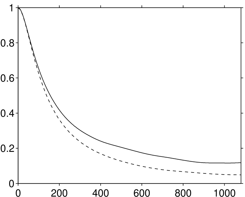
$r_{\mathrm{x}}^{+}$

$\quad R_{\mathrm{u^{\prime}u^{\prime}}}(r_{x},y^{+}\!=\!10,0)$

$\quad R_{\mathrm{u^{\prime}u^{\prime}}}(0,y^{+}\!=\!10,r_{z})$

$(b)$

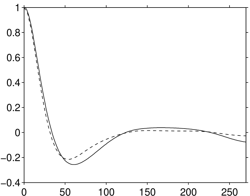
$r_{\mathrm{z}}^{+}$

$(c)$

$k_{\mathrm{x}}\,D$

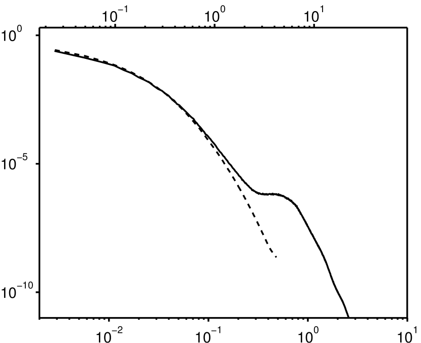
$k_{\mathrm{x}}^{+}$

$E_{\mathrm{u^{\prime}u^{\prime}}}(k_{x},y^{+}\!=\!10,0)/\langle u^{\prime}u^{\prime}\rangle$

$E_{\mathrm{u^{\prime}u^{\prime}}}(0,y^{+}\!=\!10,k_{z})/\langle u^{\prime}u^{\prime}\rangle$

$(d)$

$k_{\mathrm{z}}\,D$

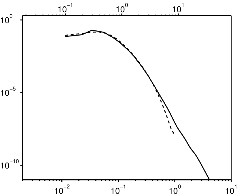
$k_{\mathrm{z}}^{+}$

Figure 11: Graphs $(a)$, $(b)$ show the auto-correlation coefficient of the streamwise velocity component as defined in (2), for separations in the streamwise and spanwise direction, respectively. The corresponding one-dimensional energy spectra are shown in graphs $(c)$ and $(d)$ as a function of the wavenumber $k_{\alpha}$ (with directional index $\alpha=1$ and $3$). Solid lines are for the present particulate flow case, dashed lines for corresponding single-phase flow.

A more sensitive measure of local flow field modification is provided by the dissipation rate of fluctuating kinetic energy, $\varepsilon=2\nu s_{ij}^{\prime}s_{ij}^{\prime}$, where $s_{ij}^{\prime}=(u_{i,j}^{\prime}+u_{j,i}^{\prime})/2$ is the fluctuating rate-of-strain tensor. A map of $\varepsilon$ is provided in figure 10$c$ for the present case and in figure 10$d$ for the corresponding single-phase flow. Note that in the particulate case, where data is generated by means of a finite-difference method on a staggered grid, consistent computation of the dissipation rate requires interpolation, thereby introducing a certain amount of smoothing. Contrarily, the single-phase data is obtained via a pseudo-spectral method in a collocated grid arrangement, where dissipation can be directly computed point-wise. Indeed, the figure shows that localized contributions to the dissipation rate can be observed in the vicinity of the phase-interfaces. However, the largest values of dissipation are in general found in regions outside the low-speed streaks, which appear not to be much affected by the presence of particles. Also, note that such instantaneous dissipation maps exhibit a considerable temporal variation due to the intermittent nature of this quantity. Therefore, a one-on-one comparison is at best qualitative. When plane-averaged and averaged in time, the contribution to dissipation stemming from the particles should become negligible, since we have seen above that the turbulent kinetic energy is practically unaffected by their presence.

The possible influence of the particles can be further quantified by analyzing the two-point auto-correlations of the streamwise velocity fluctuations defined as

$$\!\!\!\!\!\!\!\!\!\!\!\!\!\!\!\!\!\!\!\!\!\!\!R_{\mathrm{u}^{\prime}\,\mathrm{u}^{\prime}}(r_{\mathrm{x}},y,r_{\mathrm{z}})=\frac{1}{L_{\mathrm{x}}L_{\mathrm{z}}\langle u^{\prime}u^{\prime}\rangle(y)}\int_{0}^{L_{\mathrm{x}}}\int_{0}^{L_{\mathrm{z}}}u^{\prime}(x,y,z)u^{\prime}(x+r_{\mathrm{x}},y,z+r_{\mathrm{z}})\,\mathrm{d}x\mathrm{d}z\,$$ (2)

where $r_{\mathrm{x}}$ and $r_{\mathrm{z}}$ are streamwise and spanwise separations, respectively, and $u^{\prime}$ refers to a velocity fluctuation with respect to the average over wall-parallel planes and time. Note, that in (2) it is not distinguished between regions of fluid or solid phase. Figure 11$a$ shows the auto-correlation coefficient of the streamwise velocity component as a function of streamwise separations at a wall distance of $y^{+}=10$ at zero spanwise separation. In addition the result from the single-phase reference case is included in the figure. At increasing separations $r_{\mathrm{x}}$ the correlation coefficient in the present case is larger than in the single-phase flow and exhibits values of $0.12$ at the largest streamwise distance compared to a value of $0.04$ in the single-phase case. Figure 11$b$ shows the correlation coefficient as a function of spanwise separation, $r_{\mathrm{z}}$ for zero streamwise separation. The magnitude and location of the minima differs, i.e. the minimum is located at $r_{\mathrm{z}}^{+}=60$ and has a value of $-0.26$ in the present case while in the single-phase flow the minimum is located at $r_{\mathrm{z}}^{+}=55$ and has a value of $-0.19$. In contrast to the single-phase flow the auto-correlation in the present case reaches positive values for $120<r_{\mathrm{z}}^{+}<230$, leading to a local maximum at $r_{\mathrm{z}}^{+}=166$ ($R_{\mathrm{u}^{\prime}\,\mathrm{u}^{\prime}}=0.04$).

Since small-scale contributions are not easily observed from the spatial correlation functions, we present the corresponding one-dimensional energy spectra in figure 11$(c,d)$. It can be seen that particles affect the distribution of kinetic energy among the scales only at scales around and below their diameter $D$. The effect is more pronounced in the streamwise direction, where a visible ‘bump’ is observed.

In conclusion, a small but distinct effect of the particles on the turbulence structure is found in the auto-correlation of the flow field close to the wall. The increase in the magnitude of the correlation coefficient of the streamwise velocity fluctuations for separation in the streamwise as well as in the spanwise direction can be explained by a stabilising effect of the particles on the near wall structures leading to somewhat more elongated flow structures.

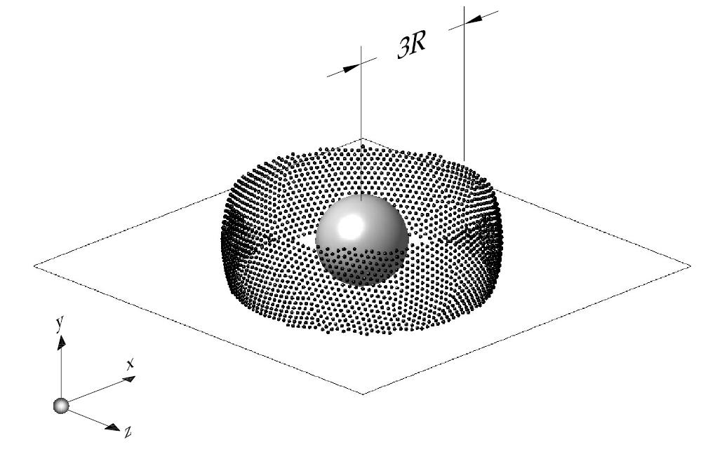
Figure 12: The spherical segment surface ${\cal S}$ over which fluid velocity is averaged in order to define a representative instantaneous velocity at the particle location. The spherical segment has a radius $R_{\mathrm{s}}=3R$. The parallel planes which define the segment are intersecting the sphere with radius $R_{s}$ at a distance equal to $R$ on either side of the center, both being parallel to the wall-plane.

3.2 Definition of the fluid velocity seen by finite-size particles

The concept of a fluid velocity “seen” by suspended particles is extensively used in the context of particulate flow systems. It represents a simplification in the sense that one supposes particles to undergo a certain forcing due to an “incoming” flow, similar to a fixed immersed object in a cross-stream, while ignoring the modification to the flow due to the particle itself. When considering point particles, particularly in the case of one-way coupling, the characteristic fluid velocity is simply taken as the fluid velocity evaluated at the particle’s location. Finite-size particles however, modify the carrier flow around them by constraining the fluid velocity at the fluid/solid interface. Consequently, there is no unique definition of a representative fluid velocity seen by finite-size particles.

$(a)$

$\tilde{z}/R$

$\tilde{x}/R$

$\tilde{x}/R$

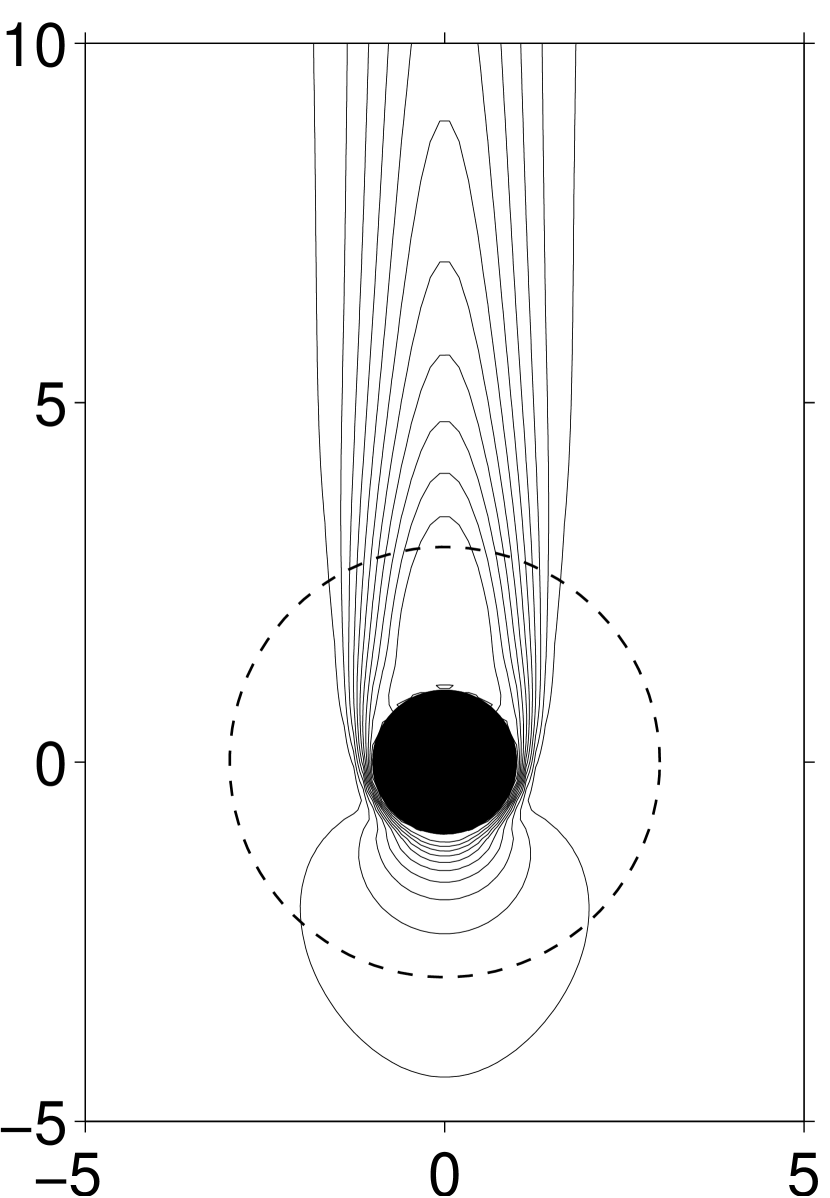
$(b)$

$\tilde{z}/R$

$\tilde{x}/R$

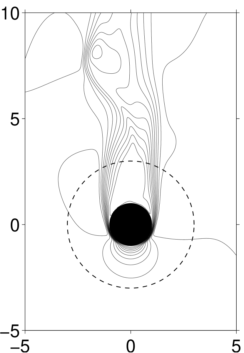
$(c)$

$\tilde{z}/R$

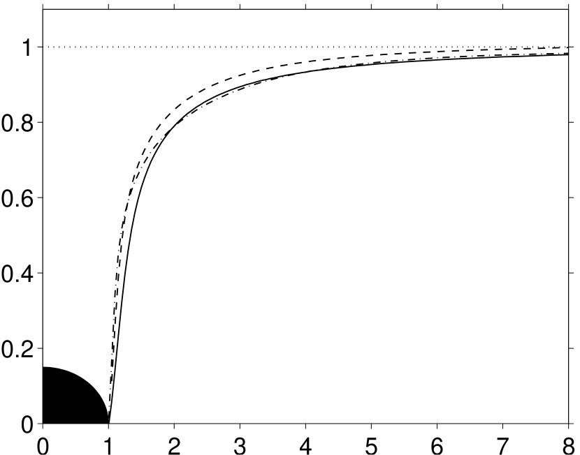
$(d)$

$R_{\mathrm{s}}/R$

${u}^{\cal S}_{\mathrm{f}}/{u}_{\mathrm{f},\infty}$

Figure 13: (a)-(c) Contour plots of instantaneous streamwise velocity fields of an unbounded flow past a fixed sphere in the steady axisymmetric and the unsteady wake regimes. (a) $Re_{\infty}=50$, (b) $Re_{\infty}=140$, and (c) $Re_{\infty}=350$. Contourlines correspond to (0:0.1:1) times the magnitude of ${u}_{\mathrm{f},\infty}$. The circle indicated by a dashed line has a radius of $3R$. (d) The computed value ${u}^{\cal S}_{\mathrm{f}}$ of the axial component of the instantaneous fluid velocity “seen by the particle”, as given by the definition (3), plotted as a function of $R_{\mathrm{s}}$. ( ) $Re_{\infty}=50$; (        ) $Re_{\infty}=140$; (     ) $Re_{\infty}=350$.

Previously, there have been several attempts to define the undisturbed fluid velocity seen by finite-size particles. Bagchi and Balachandar (2003) simulated isotropic turbulence swept past a fixed sphere and Zeng et al. (2008) considered non-periodic channel flow with a fixed sphere. In both of these studies, the undisturbed fluid velocity at a particle location was estimated from the fluid velocity at the same location of a separately computed turbulent flow without the sphere. Merle et al. (2005), using Taylor hypothesis, approximated the undisturbed fluid velocity at a certain downstream location ($2.5D$ from the center of the particle) and at an earlier time. Note that all of these three studies considered fixed spheres. The authors remark that these approaches are only adequate for estimating the velocity seen by particles with sizes smaller than the flow scales and they question the applicability in the case of finite-size particles. Lucci et al. (2010) considered mobile finite-size particles in decaying isotropic turbulence in the absence of gravity. They defined the characteristic fluid velocity as an average over a small spherical cap with center located in the direction given by the particle velocity (measured in an inertial reference frame). In turbulent flows, however, this choice of directional bias appears questionable since it is the relative (not the absolute) velocity which distinguishes the direction of the “incoming” fluid flow.

Here, we propose a definition for the characteristic fluid velocity in the vicinity of the particles which avoids the directional assumption. The instantaneous fluid velocity $\mathbf{u}^{\cal S}_{\mathrm{f}}$ in the vicinity of the $i$th particle is approximated by the average of the velocity of the fluid located on a spherical surface ${\cal S}$ of radius $R_{s}$ centered at the particle’s center location $\mathbf{x}^{(i)}_{\mathrm{p}}$. In order to avoid sampling bias due to the inhomogeneity in wall-normal direction in the considered channel flow, the averaging spherical surface is trimmed by two wall-parallel planes at one particle radius $R$ below and above the center leading to the definition of a spherical surface segment as shown in figure 12. Any point $l$ on this surface has a position vector $\mathbf{x}_{l}^{(i)}(t)=\mathbf{x}_{\mathrm{p}}^{(i)}(t)+R_{\mathrm{s}}\mathbf{n}$ where $\mathbf{n}$ is an outward pointing unit vector normal to ${\cal S}$ at $\mathbf{x}_{l}^{(i)}(t)$. With the surface ${\cal S}$ discretized by $N_{\mathrm{l}}$ Lagrangian marker points, the average velocity of the fluid instantaneously located on the surface ${\cal S}$ is defined as (using the indicator function $\phi_{\mathrm{f}}(\mathbf{x},t)$ defined in 18):

$$\mathbf{u}_{\mathrm{f}}^{\cal S}(\mathbf{x}_{\mathrm{p}}^{(i)},R_{\mathrm{s}},t)=\frac{1}{n_{\cal S}^{(i)}(t)}\sum_{l=1}^{N_{\mathrm{l}}}\phi_{\mathrm{f}}(\mathbf{x}^{(i)}_{l}(t),t)\mathbf{u}_{\mathrm{f}}(\mathbf{x}^{(i)}_{l}(t),t)\quad\forall\,i=1\ldots N_{\mathrm{p}}\,,$$ (3)

where the counter $n_{\cal S}^{(i)}(t)$ is defined as

$$n_{\cal S}^{(i)}(t)=\sum_{l=1}^{N_{\mathrm{l}}}\phi_{\mathrm{f}}(\mathbf{x}^{(i)}_{l}(t),t)\,.$$ (4)

Note that the presence of $\phi_{\mathrm{f}}$ in (3) avoids undesired sampling of velocity data inside a neighboring solid particle. Generally $\mathbf{x}_{l}^{(i)}(t)$ does not coincide with the fixed Cartesian grid where the velocity field $\mathbf{u}_{\mathrm{f}}(\mathbf{x},t)$ is available. Therefore we determine $\mathbf{u}_{\mathrm{f}}(\mathbf{x}_{l}^{(i)}(t),t)$ by a trilinear interpolation from $\mathbf{u}_{\mathrm{f}}$ values at the grid nodes in the fluid domain $\Omega_{\mathrm{f}}(t)$.

The choice of the radius $R_{\mathrm{s}}$ needs to meet two requirements. First, it should be chosen sufficiently large in order to avoid a possible influence of the particle’s own near field upon the computed value of the surrounding fluid velocity. Secondly, the value of $R_{\mathrm{s}}$ should not be chosen too large such that the resulting $\mathbf{u}_{\mathrm{f}}^{\cal S}$ is still of direct relevance to the motion of the $i$th particle.

$(a)$

$[\langle u_{\mathrm{f}}\rangle;\langle u_{\mathrm{p}}\rangle;\langle u^{\cal S}_{\mathrm{f}}\rangle]^{+}$

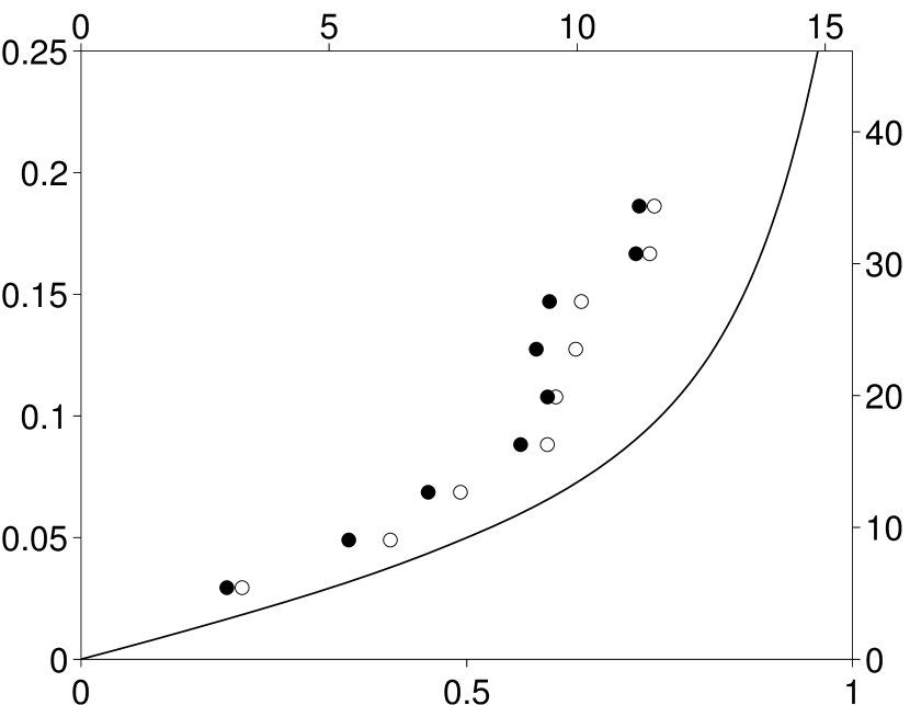
$[\langle u_{\mathrm{f}}\rangle;\langle u_{\mathrm{p}}\rangle;\langle u^{\cal S}_{\mathrm{f}}\rangle]/u_{\mathrm{b}}$

$y/h$

$y^{+}$

$(b)$

$[\langle u_{\mathrm{rel}}^{\cal S}\rangle;u_{\mathrm{lag}}]^{+}$

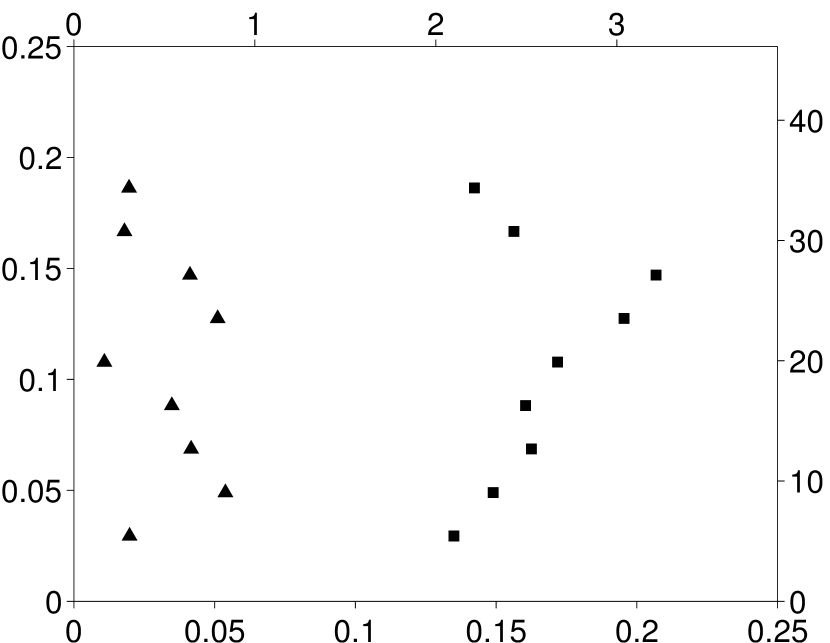
$[\langle u_{\mathrm{rel}}^{\cal S}\rangle;u_{\mathrm{lag}}]/u_{b}$

$y/h$

$y^{+}$

Figure 14: (a) Wall-normal profile of the mean streamwise fluid velocity $\langle u_{\mathrm{f}}\rangle$ ( ); the mean streamwise particle velocity $\langle u_{\mathrm{p}}\rangle$ ($\bullet$); and the mean streamwise fluid velocity in the vicinity of the particles $\langle u^{\cal S}_{\mathrm{f}}\rangle$ as defined in (3)($\circ$). (b) Wall-normal profile of the average streamwise relative velocity between the phases $\langle u_{\mathrm{rel}}^{\cal S}\rangle$ as defined in (5) ($\blacktriangle$), as well as the apparent velocity lag $u_{\mathrm{lag}}=\langle u_{\mathrm{f}}\rangle-\langle u_{\mathrm{p}}\rangle$ ($\scriptstyle\blacksquare$). In both figures, outer units are shown in the left and bottom axes and wall units in the right and top axes.

3.2.1 Testing the definition in uniform unbounded flow past a fixed sphere

In order to define a reasonable value for $R_{\mathrm{s}}$, we have applied definition (3) to resolved numerical data of a uniform unbounded flow past a fixed sphere. In this simple flow the relative velocity is equal to the incoming fluid velocity ${u}_{\mathrm{f},\infty}$. Therefore, this test case allows to estimate the smallest value of $R_{\mathrm{s}}$ which yields a sufficiently close approximation of the relative velocity, i.e. for which ${u}_{\mathrm{f}}^{\cal S}\approx{u}_{\mathrm{f},\infty}$. Here the only parameter is the Reynolds number based on the particle diameter and the incoming flow velocity, $Re_{\infty}={u}_{\mathrm{f},\infty}D/\nu$, for which we have chosen three values, namely $Re_{\infty}=50$, $Re_{\infty}=140$ (both in the steady axisymmetric wake regime), and $Re_{\infty}=350$ in the unsteady vortex shedding regime (see e.g. Johnson and Patel, 1999, for details on the structure of wakes behind spheres). Please note that the value of the Reynolds number based on particle diameter and the apparent velocity lag ($Re_{\mathrm{lag}}=u_{\mathrm{lag}}D/\nu$) in the horizontal channel flow considered in the main part of this manuscript is in the range of $15$ to $20$. Returning to the fixed sphere in unbounded uniform flow, snapshots of the velocity field in a plane through the center of the sphere are depicted in figure 13. It should be mentioned that in this unbounded flow configuration trimming the spherical averaging surface is not necessary. However, for reasons of consistency with the application of definition (3) to wall-bounded flow, we have performed the averaging over the previously defined spherical surface segment (cf. figure 12).

Figure 13d shows the average value of the instantaneous fluid velocity as defined by (3) while varying the value of $R_{\mathrm{s}}$. Note that in the unsteady case ($Re_{\infty}=350$) an average in time over several flow fields was performed. As expected, the value of the fluid velocity defined in (3) tends towards the value of the incoming fluid velocity ${u}_{\mathrm{f},\infty}$ for large values of $R_{\mathrm{s}}$. As $R_{\mathrm{s}}$ tends towards $R$, the surrounding fluid appreciates the presence of the sphere and ${u}_{\mathrm{f}}^{\cal S}$ tends to zero due to the no-slip condition. Depending on the Reynolds number, the degree to which the computed value of the surrounding fluid velocity is affected by the presence of the sphere varies somewhat. However, it is seen that for all the three cases considered, approximately 90% of the value of the incoming flow velocity is obtained at a distance of $3R$ from the particle center. Therefore, based on the above results, we define the velocity “seen” by the finite-size particles through (3) with a choice of $R_{\mathrm{s}}=3R$. Note that a similar analysis of the fluid velocity field in the vicinity of a single fixed particle in forced turbulence has been performed by Naso and Prosperetti (2010).

3.2.2 The contribution of the mean relative velocity to the apparent velocity lag

After having found a method to determine the fluid velocity “seen” by a particle as given in (3), we can now define an instantaneous relative velocity for the $i$th particle, viz.

$$\mathbf{u}^{\cal S}_{\mathrm{rel}}(i,R_{s},t)=\mathbf{u}_{\mathrm{f}}^{\cal S}(\mathbf{x}^{(i)}_{\mathrm{p}},R_{\mathrm{s}},t)-\mathbf{u}^{(i)}_{\mathrm{p}}(t)\,,$$ (5)

with $R_{\mathrm{s}}=3R$. The average over all particles and time of $u_{\mathrm{f}}^{\cal S}$ and of $u_{\mathrm{rel}}^{\cal S}$ can be computed by the averaging operator (26) defined in B.3. Note that the values of $\langle u_{\mathrm{f}}^{\cal S}\rangle$ and $\langle u_{\mathrm{rel}}^{\cal S}\rangle$ discussed in the following stem from 70 instantaneous flow fields. Therefore the statistics are based on a smaller number of samples than those computed from data collected during run-time, e.g. the values of $\langle u_{\mathrm{f}}\rangle$ and $\langle u_{\mathrm{p}}\rangle$. Furthermore, we have verified that the following results are not very sensitive to a variation of the chosen value of $R_{s}$.

Figure 14$a$ shows $\langle u_{\mathrm{f}}^{\cal S}\rangle$ in comparison to $\langle u_{\mathrm{f}}\rangle$ and $\langle u_{\mathrm{p}}\rangle$ in the wall region $y^{+}<36$. The figure clearly demonstrates that the average velocity of the fluid in the vicinity of the particles $\langle u_{\mathrm{f}}^{\cal S}\rangle$ is significantly smaller than the unconditioned fluid velocity $\langle u_{\mathrm{f}}\rangle$ and that the former is comparable in magnitude to the mean particle velocity $\langle u_{\mathrm{p}}\rangle$ for most of the wall-normal interval. Figure 14$b$ which shows $\langle u_{\mathrm{rel}}^{\cal S}\rangle$ in comparison to $u_{\mathrm{lag}}$ highlights this finding. At $y^{+}\approx 5$, which holds most of the particles, $\langle u_{\mathrm{rel}}^{\cal S}\rangle\approx 0.31u_{\tau}$ which is considerably smaller than $u_{\mathrm{lag}}\approx 2.10u_{\tau}$. At larger wall-normal distances the value of $\langle u_{\mathrm{rel}}^{\cal S}\rangle$ increases slightly, attaining a maximum value of approximately $0.91u_{\tau}$ although a clear trend with wall-normal distance is difficult to infer due to the decrease of the number of data samples away from the wall (cf. figure 4). However, it is beyond doubt that for the considered wall distances $\langle u_{\mathrm{rel}}^{\cal S}\rangle$ is considerably smaller than $u_{\mathrm{lag}}$. The relative particle Reynolds number $Re_{\mathrm{rel}}=\langle u_{\mathrm{rel}}^{\cal S}\rangle D/\nu$ for the particles closest to the wall has a value $Re_{\mathrm{rel}}\approx 2.2$ which is much smaller than $Re_{\mathrm{lag}}\approx 15$. The very small value of $Re_{\mathrm{rel}}$ indicates that there are no substantial particle-induced wakes, which is confirmed by the conditionally averaged flow field around the particles discussed in more detail in § 3.4. It can be concluded from the present results that the dominant contribution to $u_{\mathrm{lag}}$ stems indeed from the preferential location of particles in the low-speed regions of the flow, in agreement with previous experimental findings (Kaftori et al., 1995b; Kiger and Pan, 2002).

Figure 15: A Voronoi tessellation of a periodic horizontal plane corresponding to the particle positions of the snapshot shown in figure 10$a$.

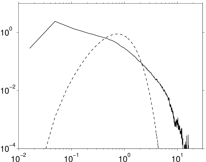
$(a)$

$A_{\mathrm{V}}/\langle A_{\mathrm{V}}\rangle$

$\quad pdf$

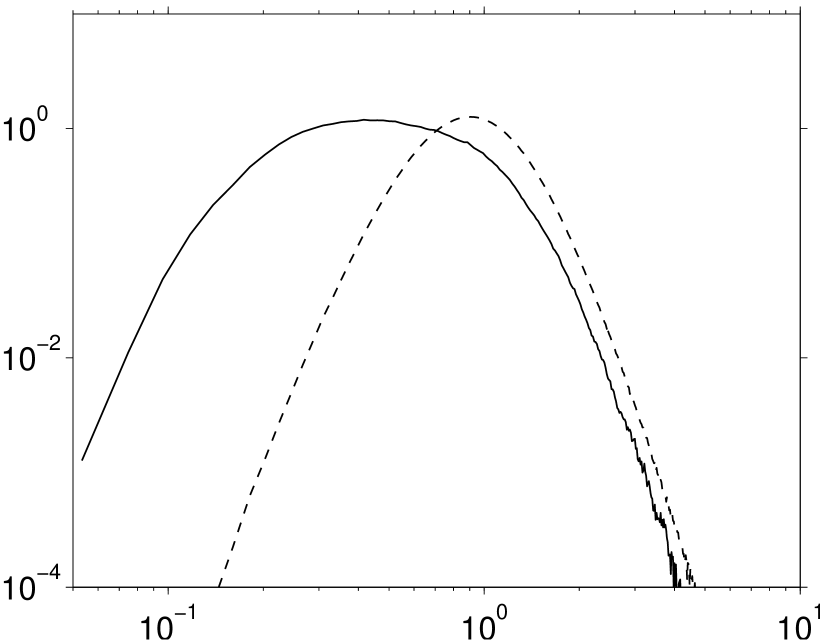
$(b)$

$l_{\mathrm{x,V}}/l_{\mathrm{z,V}}$

$\quad pdf$

Figure 16: Probability density function of (a) the normalized Voronoi cell areas and (b) the ratio of the distances between the extreme streamwise and spanwise extents of the Voronoi cells. The dashed lines represent corresponding distributions of particle positions generated randomly with uniform probability.

3.3 Distribution and motion of particles at the bottom wall

As a combined effect of gravity and turbulent dynamics, particles in the present study are observed to spend most of their time residing near the bottom wall. Occasionally they are entrained and lifted up by the carrier flow and either return to the bottom or are ejected to the outer region of the flow. During their residence time at the wall, the behaviour of particles (their streamwise and spanwise motion as well as their spatial distribution) is closely related to the dynamics of the near wall coherent flow structures. In this section we study the near-wall particle behaviour by analyzing particle positions and velocities.

It is clearly observable from the instantaneous flow field and from the corresponding particle positions shown in figure 10$a$ that particles form elongated structures, resembling streamwise aligned chains. Visualization of sequences of such images shows that these particle clusters remain in the form of quasi-streamwise aligned streaky structures which maintain a coherence over substantial time scales. In line with previous experimental findings (Kaftori et al., 1995a; Niño and García, 1996), these particle streaks are observed to reside preferentially in low-speed fluid regions. Animations show that, during their travel downstream, particles remain in these relatively quiescent low-speed streaks for relatively long time intervals, exhibiting only slight spanwise ondulations. In those animations it can also be seen that incoming sweeps of high momentum fluid sometimes act to dissolve the particle accumulations, after which those particles relatively quickly migrate back to a neighboring low-speed region.

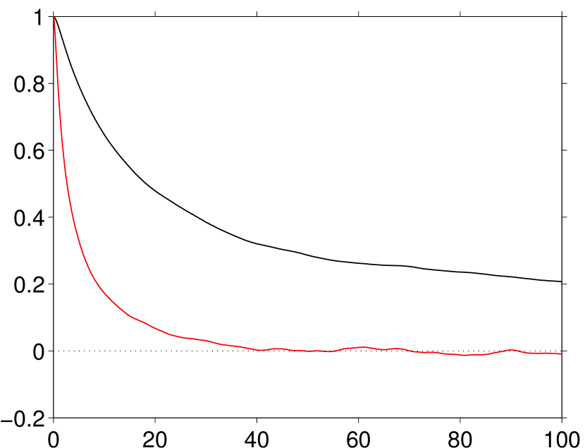
$\tau_{\mathrm{sep}}/T_{\mathrm{b}}$

$\quad R_{\mathrm{L},Q_{\mathrm{V}}}$

Figure 17: Lagrangian autocorrelation as a function of time lag $\tau_{\mathrm{sep}}$ for the Voronoi area ( ) and the Voronoi cell aspect ratio (  ).

As a quantitative measure of the spatial distribution of particles, we have carried out a cluster analysis based on Voronoi diagrams. Voronoi diagrams are tessellations which partition a space based on a set of given center positions (the ’sites’) into regions such that each point inside a given region is closer to the region’s site than to any other site (Okabe et al., 1992). Voronoi diagram analysis is widely utilized in many scientific areas and has been introduced as a tool for the analysis of preferential particle concentration in turbulent flows (Monchaux et al., 2010, 2012).

In order to investigate the spatial distribution of particles in the immediate vicinity of the wall, a horizontal plane of the bi-periodic domain is tessellated based on instantaneous streamwise and spanwise positions of all particles whose center is located at a wall-normal distance within one particle diameter from the bottom wall. Each of the resulting Voronoi regions has an area $A_{\mathrm{V}}^{(i)}$ associated to the $i$th particle. The example given in figure 15 demonstrates that the tesselation is area-filling, taking into account the bi-periodicity. The inverse of a Voronoi cell area is directly related to the local particle concentration: small areas correspond to high local particle concentration and large Voronoi cell areas to voids. We have analyzed the distribution of these areas compared to the distribution of the Voronoi areas associated with randomly-positioned particle sets. The p.d.f. of the Voronoi areas (normalized by the mean value) of randomly positioned points is independent of the particle number density (Ferenc and Néda, 2007). However, finite-size particles have the constraint that they cannot overlap, and at close-packing (the maximum possible particle number density), all Voronoi areas are identical and have a Dirac delta distribution. Here we generate reference data from a sufficiently large number of randomly-positioned particle sets (with uniform probability in space) applying the constraint that they do not overlap and adopting a particle number density equal to the one of the present flow case.

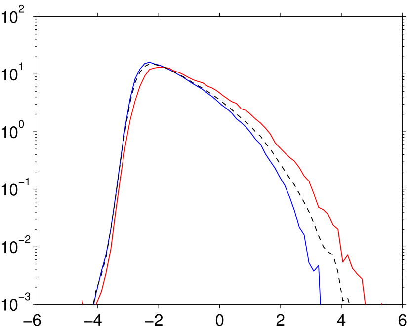
$[u_{\mathrm{p}}-\langle u_{\mathrm{f}}\rangle]^{+}$

$\quad pdf$

Figure 18: P.d.f.s of the streamwise particle velocity relative to the mean flow $u^{(i)}_{\mathrm{p}}(t)-\langle u_{\mathrm{f}}\rangle(y^{(i)}_{\mathrm{p}}(t))$ conditioned upon the Voronoi cell area $A^{(i)}_{\mathrm{V}}(t)$ of all particles whose centers are located at a wall-normal distance from the bottom $y^{(i)}_{\mathrm{p}}(t)<D$. The color coding represents: conditional p.d.f. of those particles such that their associated Voronoi cell area $A^{(i)}_{\mathrm{V}}(t)<A^{c}_{\mathrm{V}}$, (  ); conditional p.d.f. of those particles such that their associated Voronoi cell area $A^{(i)}_{\mathrm{V}}(t)>A^{v}_{\mathrm{V}}$, (  ). The dashed line corresponds to the unconditioned p.d.f. of the same quantity in this wall-normal interval. Note that the p.d.f.s are not centered about their respective mean.

Figure 16(a) shows the p.d.f. of the normalized Voronoi areas computed from 20314 snapshots of the particle ‘field’. A significant deviation of the p.d.f. from the corresponding randomly-positioned particles indicates that the particle distribution at the bottom wall is far from random – as already observed visually, e.g. in figure 15. The DNS data exhibits a much higher probability of finding very small and very large Voronoi areas than in a random case with uniform probability. The fact that there is a high probability for particles in the present case to be associated with very small Voronoi cell areas indicates that, consistent with the visual evidence, particles have a clear tendency to accumulate.

In order to provide a measure of the anisotropy of particle accumulation regions, we have further analyzed the shape of the Voronoi cells. More specifically, we have examined the slenderness (i.e. the aspect ratio) of these regions by computing the ratio between the largest extent of each Voronoi cell in the streamwise direction ($l_{\mathrm{x,V}}$) and in the spanwise direction ($l_{\mathrm{z,V}}$). Figure 16(b) shows the p.d.f. of the aspect ratio of the Voronoi cells along with the p.d.f. of the same quantity for the randomly-positioned particles. Again, there is an appreciable difference between the two p.d.f.s. On average, the Voronoi regions associated with the particles from the present case have a smaller aspect ratio ($\langle l_{\mathrm{x,V}}/l_{\mathrm{z,V}}\rangle=0.722$) when compared to that of the random case ($\langle l_{\mathrm{x,V}}/l_{\mathrm{z,V}}\rangle=1.062$ – which should tend to unity when increasing the sampling size). Moreover, there is a higher probability of finding a small aspect ratio than in the random case and vice versa. This indicates that the regions are significantly squeezed (stretched) in the streamwise (spanwise) directions which means that particles are more likely to be streamwise aligned than aligned along the spanwise axis. Therefore, the Voronoi cell aspect ratio analysis confirms the visual observation of alignment of particles into streamwise elongated ‘streaks’.

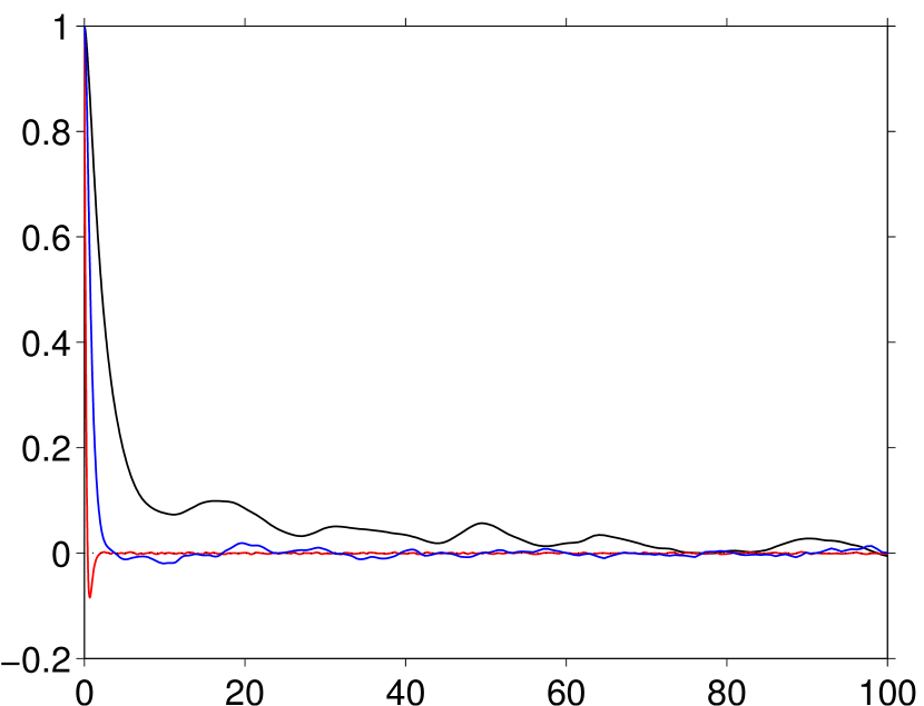
$\tau_{\mathrm{sep}}/T_{\mathrm{b}}$

$\quad R_{\mathrm{L},u_{\mathrm{p},\alpha}}$

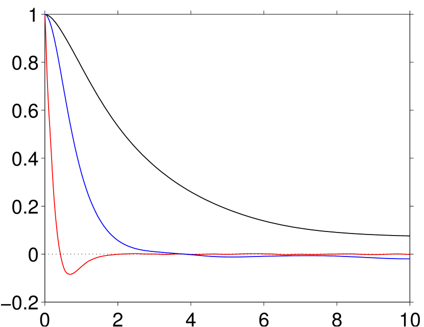
Figure 19: Lagrangian autocorrelation as a function of time lag $\tau_{\mathrm{sep}}$ for the velocity of all particles whose centers are located at a wall-normal wall distance $y^{(i)}_{\mathrm{p}}(t)<D$. The color code indicates: ( ) streamwise component, $\alpha=1$; ( ) wall-normal component, $\alpha=2$; ( ) spanwise component, $\alpha=3$. The insert shows a closeup of the same data for small separation times.

Furthermore, we have tracked the Voronoi area and Voronoi aspect ratio associated to each particle in time in order to study the behaviour of these quantities in a Lagrangian sense. The Lagrangian autocorrelation function of a Voronoi cell quantity as a function of separation time $\tau_{\mathrm{sep}}$ can be defined as

$$R_{\mathrm{L},Q_{\mathrm{V}}}(\tau_{\mathrm{sep}})=\frac{\langle Q^{\prime}_{\mathrm{V}}(t)\,Q^{\prime}_{\mathrm{V}}(t+\tau_{\mathrm{sep}})\rangle}{\langle Q^{\prime}_{\mathrm{V}}(t)\,Q^{\prime}_{\mathrm{V}}(t)\rangle}\,,$$ (6)

where the quantity $Q_{\mathrm{V}}(t)$ is either the Voronoi area or the Voronoi aspect ratio at time $t$ and $Q^{\prime}_{\mathrm{V}}(t)=Q_{\mathrm{V}}(t)-\langle Q_{\mathrm{V}}\rangle$. The averaging in (6) is performed over all particles and over time, where segments of time signals are used for which the considered particle resides close to the wall, i.e. $y_{p}^{(i)}(t^{\prime})<D\ \forall\,t^{\prime}\in[t,t+\tau_{sep}]$ .

Figure 17 shows the quantity $R_{\mathrm{L},Q_{\mathrm{V}}}$ as a function of $\tau_{\mathrm{sep}}$ for both the Voronoi area and Voronoi aspect ratio. The data shown in figure 17 demonstrates that the spatial particle distribution is indeed highly persistent in time. The Voronoi cell area is still significantly correlated (with a coefficient value of approximately $0.2$) even after $100$ bulk time units. The Voronoi cell aspect ratio, on the other hand, changes much faster, with the correlation coefficient practically vanishing after approximately $40$ bulk time units. The Taylor micro scale (given by the osculating parabola at zero separation) measures $5.2\,T_{\mathrm{b}}$ ($1.3\,T_{\mathrm{b}}$) for the cell area (cell aspect ratio). The difference in time scales measured for these two quantities becomes obvious from a closer inspection of time sequences of Voronoi diagrams. Therein it can be observed that while particles typically remain located for a long time inside one specific accumulation region, the shape of their associated Voronoi cell fluctuates significantly without necessarily changing the cell’s area.

The intersection points of the two curves in figure 16(a) (DNS data versus random particle distribution) can be used to define an objective criterion for determining whether a particle is located inside a cluster or inside a void (Monchaux et al., 2010). For this purpose, the cell area corresponding to the lower ($A^{c}_{\mathrm{V}}$) and upper ($A^{v}_{\mathrm{V}}$) intersection points in that diagram are considered as threshold values: all particles with associated Voronoi cell area lower than $A^{c}_{\mathrm{V}}$ are considered to reside in a cluster, those with a volume larger than $A^{v}_{\mathrm{V}}$ are related to voids. We have computed for each particle the number of times it crosses these threshold values and we have determined the duration of all temporal intervals during which the Voronoi cell area is continuously below (above) the lower (upper) threshold value. This type of study allows us to estimate the residence time of particles in a region with an ‘extreme’ concentration (e.g. a cluster or a void). It turns out that the average residence time in a cluster (void) is approximately $7.8T_{\mathrm{b}}$ ($6.9T_{\mathrm{b}}$) while the average frequency of a particle entering a cluster (void) region is $0.06/T_{\mathrm{b}}$ ($0.02/T_{\mathrm{b}}$). Concerning the Voronoi cell aspect ratio (which exhibits a single intersection point, cf. figure 16$b$), one can define a threshold below which the Voronoi cell’s shape can be considered as spanwise elongated. The analysis yields an average temporal interval of $5.5T_{\mathrm{b}}$ during which a particle has an associated spanwise elongated Voronoi cell.

The data from the Voronoi analysis can be further utilized for the purpose of conditionally averaging the Lagrangian particle quantities. To this end we have computed the difference between the streamwise component of the instantaneous particle velocity and the mean fluid velocity at the same wall-normal distance, i.e. $u^{(i)}_{\mathrm{p}}(t)-\langle u_{\mathrm{f}}\rangle(y^{(i)}_{\mathrm{p}}(t))$ for the $i$th particle. The p.d.f. of this velocity difference is shown in figure 18 for those particles whose center is located within one diameter of the wall plane. The curve for the unconditioned quantity is clearly skewed towards positive values (i.e. large positive fluctuations are more probable than large negative ones). Conditioning the same quantity upon the Voronoi cell area has a substantial effect, which is, however, mostly limited to a different probability for observing positive values. In particular, particles located in clusters (voids) have a significantly lower (higher) probability to exhibit streamwise velocities which exceed the average fluid velocity. One can conclude from this analysis that particles located in void regions have a higher tendency to be located in high-speed fluid regions than particles located in accumulation regions.

Finally, we consider the auto-correlation function of the particle velocity components, which is defined as

$$R_{\mathrm{L},u_{\mathrm{p}},\alpha}(\tau_{\mathrm{sep}})=\frac{\langle u_{\mathrm{p},\alpha}^{\prime}(t)\,u_{\mathrm{p},\alpha}^{\prime}(t+\tau_{\mathrm{sep}})\rangle}{\langle u_{\mathrm{p},\alpha}^{\prime}(t)\,u_{\mathrm{p},\alpha}^{\prime}(t)\rangle}\qquad\forall\,\alpha=1,2,3\,,$$ (7)

in analogy to (6). Note that again only those data points are considered which correspond to particles remaining near the wall during the entire separation interval (i.e. with center $y_{c}^{(i)}(t^{\prime})<D\ \forall\,t^{\prime}\in[t,t+\tau_{sep}]$), consistent with the previous discussion. Figure 19 shows that the wall-normal particle velocity component decorrelates fastest, followed by the spanwise component and (with a much longer time scale) the streamwise component. The corresponding Taylor microscales measure $1.41\,T_{\mathrm{b}}$, $0.15\,T_{\mathrm{b}}$ and $0.75\,T_{\mathrm{b}}$ for the streamwise, wall-normal and spanwise components, respectively. The longer time scale of the streamwise particle velocity is owed to the anisotropy of the near-wall turbulence, i.e. the persistence of velocity streaks affecting the particle motion. A similar observation has been made in vertical particulate channel flow (García-Villalba et al., 2012). Contrary to that configuration, however, the wall-normal component behaves quite differently from the spanwise component in the present case. In particular, the curve for $R_{\mathrm{L},u_{\mathrm{p}},2}$ exhibits significant negative correlations at small separation times, with the first change of sign taking place at $\tau_{\mathrm{sep}}=0.43\,T_{\mathrm{b}}$. This feature is absent in the corresponding correlation curve in the case of the vertical particulate channel, and it must therefore be due to the action of gravity in the wall-normal direction. More specifically, gravity is counteracting any particle motion away from the wall, leading to wall-normal particle velocities which often exhibit a reversal of sign after relatively short times.

$\tilde{x}^{+}$

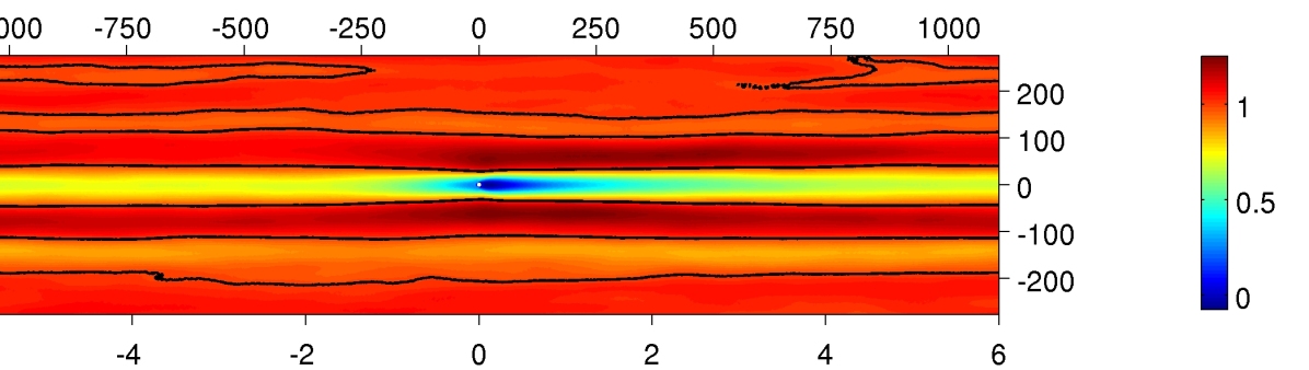
$\tilde{x}/h$

$\quad\tilde{z}/h$

$\quad\tilde{z}^{+}$

Figure 20: The average of the particle-conditioned relative streamwise velocity $\tilde{u}_{\mathrm{r}}$ (defined in equation 10), normalized by $u_{lag}$ in the near wall region. The solid black lines correspond to a value of unity.

$(a)$

$\tilde{x}^{+}$

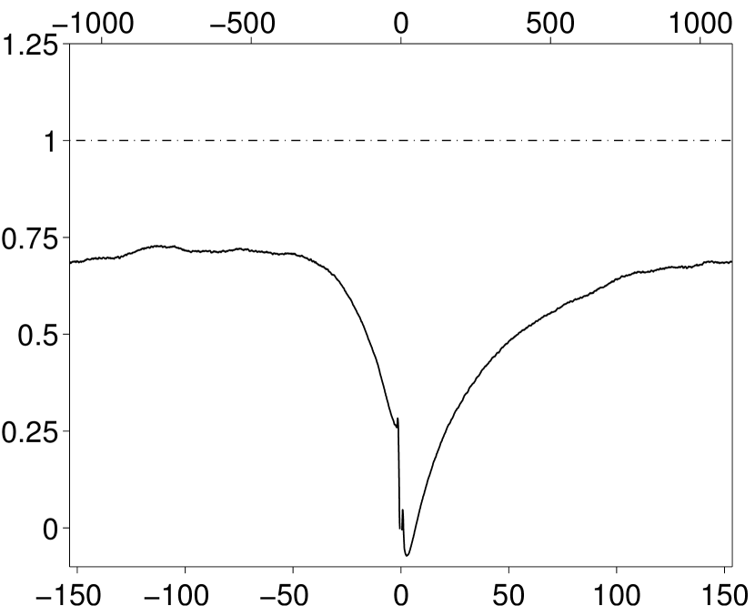
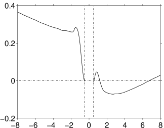
$\tilde{x}/D$

$\tilde{u}_{\mathrm{r}}/u_{\mathrm{lag}}$

$(b)$

$\tilde{z}^{+}$

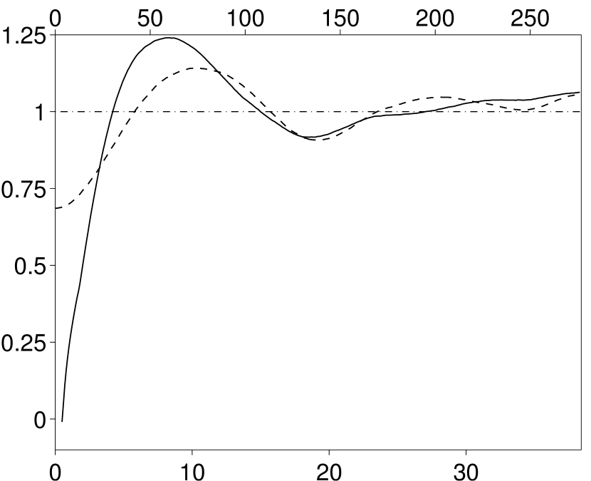
$\tilde{z}/D$

$\tilde{u}_{\mathrm{r}}/u_{\mathrm{lag}}$

Figure 21: The same quantity $\tilde{u}_{\mathrm{r}}/u_{\mathrm{lag}}$ as in figure 20. (a) shows a streamwise profile through the particle center ($\tilde{z}=0$), with the insert presenting a zoom around the particle location. (b) shows spanwise profiles through the particle center (at $\tilde{x}=0$, solid line) and at $\tilde{x}=6h$ (dashed line). Note that the data in (b) is symmetric with respect to $\tilde{z}=0$.

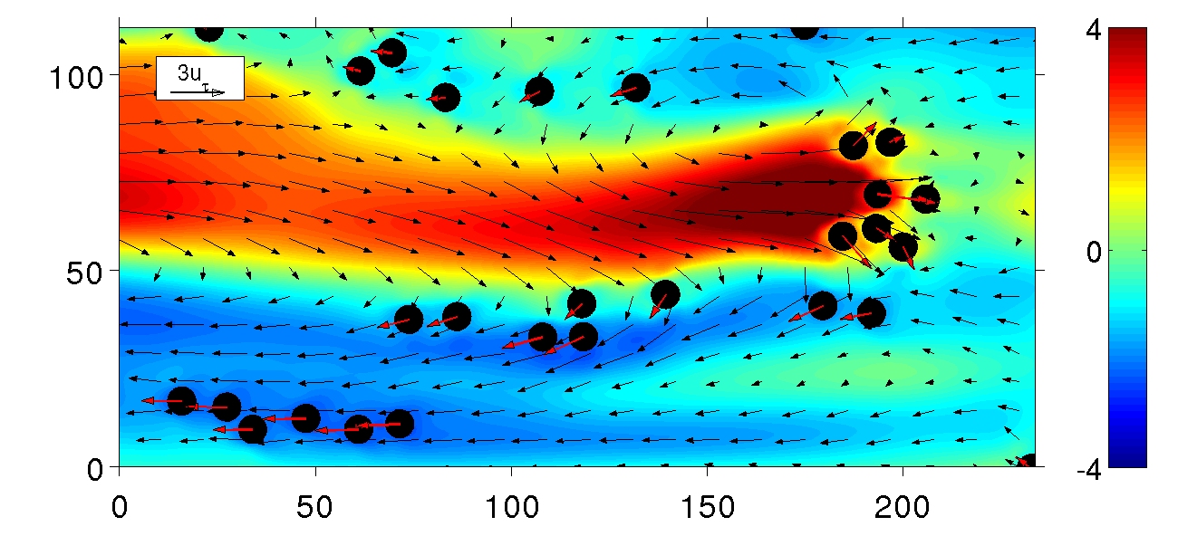
$x^{+}$

$z^{+}$

$\displaystyle\frac{u_{\mathrm{f}}^{\prime}}{u_{\tau}}$

Figure 22: Instantaneous velocity fluctuations of the fluid and the particle phase in a wall-parallel plane at $y^{+}=5$ indicated by the black (fluid) and red (particles) arrows. The colorplot represents the streamwise component of fluid velocity fluctuation, normalized by the friction velocity ($u_{\mathrm{f}}^{\prime}/u_{\tau}$). Note that backward pointing arrows do not correspond to upstream motion. In fact, upstream particle motion has not been observed in the present case. The graph shows only a small part of the entire plane, and the fluid velocity vectors have only been plotted at every 15th (10th) grid point in the $x$ ($z$) direction.

3.4 Particle-conditioned relative velocity field

In this section we discuss the fluid velocity field conditioned upon the presence of the particles. This analysis provides a quantitative measure of the spatial distribution of the low- and high-speed fluid regions with respect to particle positions. First, we define the instantaneous relative velocity field with respect to the $l$th particle as

$$\mathbf{u}^{(l)}_{r}(\tilde{\mathbf{x}}^{(l)},t)=\mathbf{u}_{f}(\tilde{\mathbf{x}}^{(l)},t)-\mathbf{u}^{(l)}_{p}(t)$$ (8)

where

$$\tilde{\mathbf{x}}^{(l)}(t)=\mathbf{x}-\mathbf{x}^{(l)}_{p}(t)$$ (9)

is an instantaneous coordinate relative to the particle’s center position. The average of the relative velocity field (with respect to the particle center) over time and over all particles located within a given wall-parallel slab $s$ is defined as follows:

$$\tilde{\mathbf{u}}_{r}(\tilde{\mathbf{x}},y^{(s)})=\langle\mathbf{u}^{(l)}_{r}(\tilde{\mathbf{x}}^{(l)},t)\rangle_{p,t}$$ (10)

where $\langle\cdot\rangle_{p,t}$ is the particle-centered field averaging operator defined in (28). We have carried out the averaging procedure by considering all particles whose centers are located at wall-normal distances within one particle diameter from the bottom wall. That is, the considered slab has a wall normal thickness of $\Delta h=D$ and its bottom edge coincides with the bottom wall. Note that this averaging procedure is identical to the one employed by García-Villalba et al. (2012) in a vertically oriented particulate channel flow.

If the particle distribution at the bottom were homogeneous, there would be no correlation between the spatial distribution of the coherent structures and the particle positions. In this case, the average of the particle-centered relative velocity component in the streamwise direction $\tilde{u}_{r}(\tilde{\mathbf{x}},y^{(s)})$ is expected to tend to the value $u_{lag}(y^{(s)})$, except in the immediate vicinity of the particle. Regardless of the particle distribution, the average relative velocity is zero at the fluid/solid interface $|\tilde{\mathbf{x}}|=D/2$, as a consequence of the no-slip condition. If, however, particles are located at certain preferred regions with respect to the flow structures, or particle are considerably affecting the flow field such that significant wakes exist behind them, then $\tilde{u}_{r}$ is expected to be significantly different from $u_{lag}$ for appreciable regions of the averaging area, except at sufficiently large distances where the averaged flow field is expected to be uncorrelated with particle positions. We can rule out the existence of significant particle-induced wakes from the analysis in § 3.2.2. Thus, locations where $\tilde{u}_{r}<u_{lag}$ correspond to regions of surrounding low-speed fluid and contrarily, locations where $\tilde{u}_{r}>u_{lag}$ correspond to high-speed fluid regions with respect to particle positions.

Figure 20 shows the quantity $\tilde{u}_{r}/u_{lag}$. It is clearly seen that on average particles are located in regions where $\tilde{u}_{r}/u_{lag}$ is below unity. The low-speed fluid region surrounding the particles on average is found to be persistent in the streamwise direction, extending for more than 1000 wall units both upstream and downstream of the particle position. It reaches the extents of the averaging plane (limited by the value of half the streamwise period of the computational domain $L_{x}/2$). Laterally however, the low-speed fluid region is seen to be correlated with the particle position for only up to about $30$ wall units both in the positive and negative spanwise directions, beyond which $\tilde{u}_{r}/u_{lag}$ rises above unity. The general pattern in figure 20 is one of spanwise alternating low- and high-speed regions correlated over the entire streamwise length of the domain. Figure 21 shows profiles of the same data on axes through the particle center both in the streamwise and spanwise directions. Note that here the spanwise profile is averaged over the positive and negative directions exploiting the symmetry of the flow. At increasing streamwise separation $\tilde{x}$ from the reference particle (figure 21$a$), $\tilde{u}_{r}$ gradually increases from its smallest value (in the vicinity of the particle) towards a finite value of approximately $0.7\,u_{lag}$ at a distance of approximately $\tilde{x}=45\,D$ ($\tilde{x}^{+}=330$) in the upstream direction and approximately $\tilde{x}=140\,D$ ($\tilde{x}^{+}=1015$) in the downstream direction. For larger distances, $\tilde{u}_{r}$ levels off at this value and does not approach unity in the present computational domain. The insert in figure 21$(a)$ reveals that the average near-field within several particle diameters exhibits some additional structure. On the upstream side, a change of slope occurs at a distance of approximately $1.5D$ from the particle center, while the downstream side features a change of sign and an interval of negatively-valued $\tilde{u}_{r}$ up to a distance of roughly $7D$. It should be noted that the asymmetry of the profile of the average relative velocity is not the signature of individual particle wakes, since the Reynolds number of the flow around the individual particles is much too low (cf. § 3.2.2) and the length scales of the asymmetric features are too large. At this point it can only be stated that the observed shape of $\tilde{u}_{r}$ on the $\tilde{x}$-axis through the particle center might be related to the preferential streamwise location of the particles with respect to the flow features of the near-wall layer. As exemplified in one snapshot in figure 22, high-speed particles are predominantly found at locations near the front of a high-velocity fluid region, thereby contributing to the asymmetry of the streamwise profile of $\tilde{u}_{r}$. This point, however, merits further investigation in the future.

In the spanwise direction (figure 21$b$), $\tilde{u}_{r}$ increases faster than in the streamwise direction, crossing the value $\tilde{u}_{r}=u_{lag}$ for the first time at a distance of approximately $\tilde{z}=4.2D$ ($\tilde{z}^{+}=30$) indicating the spanwise extent of the low-speed fluid regions. The particle-conditioned relative velocity $\tilde{u}_{r}$ attains a maximum value of $1.2u_{lag}$ at a distance of approximately $\tilde{z}=8.2D$ ($\tilde{z}^{+}=60$); this characterizes the lateral distance at which the neighbouring high-speed fluid region is strongly correlated with the particle position. For larger spanwise distances $\tilde{z}$, $\tilde{u}_{r}/u_{lag}$ oscillates with a small amplitude around unity reflecting the alternating nature of the low- and high-speed fluid regions.

It can be concluded that the spatial distribution of the coherent structures exhibits a strong correlation with particle positions almost throughout the entire streamwise and spanwise extent of the computational domain. A computational domain with dimensions much superior to those adopted in the present study would be required if a full decorrelation were desired.

3.5 Conditional average of the local volumetric particle concentration

In § 3.3 it has been quantitatively shown through Voronoi analysis that particles are inhomogeneously distributed and that they tend to be streamwise aligned. Furthermore, in § 3.4, it has been shown that the most probable position of a near-wall particle is inside a low-speed fluid region. Here, we investigate the spatial distribution of the local volumetric particle concentration conditioned to particle positions. This type of analysis provides additional information on the spatial pattern of particle accumulations/voids.

$(a)$

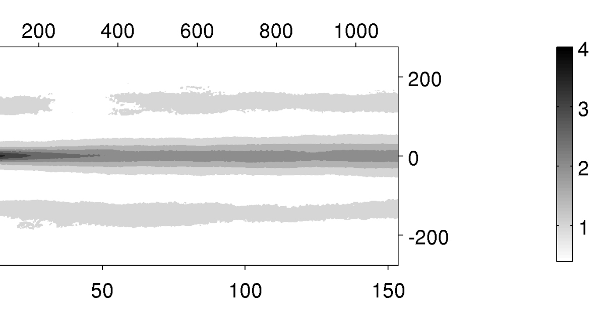
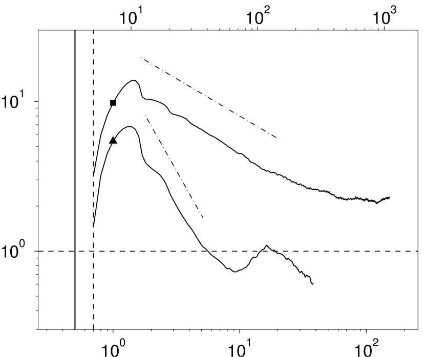
$\tilde{z}/D$ $\tilde{x}^{+}$ $\tilde{x}/D$ $\tilde{z}^{+}$               $\displaystyle\frac{\tilde{\psi}}{\langle\psi\rangle}$
                     $(b)$ $\tilde{\psi}/\langle\psi\rangle$ $\tilde{x}^{+},\tilde{z}^{+}$ $\tilde{x}/D,\tilde{z}/D$

Figure 23: (a) Contours of the conditional local particle concentration normalized by the mean solid volume fraction ($\tilde{\psi}/\langle\psi\rangle$) averaged over all particles which are located within the near-wall region ($y_{\mathrm{p}}<D$), as defined in (13). Only half of the averaging plane is shown due to symmetry. Contour levels correspond to values (1:0.5:4). The graph in (b) shows $\tilde{\psi}(\tilde{x},0,0,y^{(s)})/\langle\psi\rangle$ (square symbol) and $\tilde{\psi}(0,0,\tilde{z},y^{(s)})/\langle\psi\rangle$ (triangular symbol), both with $s=2$. The vertical solid line indicates the extent of the reference particle’s surface, and the vertical dashed line gives the distance $|\tilde{\mathbf{x}}|=D/2+2\Delta x$ from the center of the reference particle which marks the limit of the range of action of the collisional force. The chain-dotted lines indicate decay rates proportional to $x^{-0.5}$ and $x^{-1.5}$.

The indicator function of the solid phase, $\psi$, is simply related to the fluid phase indicator function $\phi_{\mathrm{f}}$ defined in (18) by the relation

$$\psi(\mathbf{x},t)=1-\phi_{\mathrm{f}}(\mathbf{x},t)\;.$$ (11)

Its average over wall-parallel planes (using nodal values of the discrete grid) and over time can be defined as

$$\langle\psi\rangle(y_{j})=1-\frac{n(y_{j})}{N_{\mathrm{t}}^{\mathrm{(p)}}N_{\mathrm{x}}N_{\mathrm{z}}}\,,$$ (12)

where $n(y_{j})$ is the discrete counter given in (19) with $N_{\mathrm{t}}$ replaced by $N_{\mathrm{t}}^{\mathrm{(p)}}$ (the number of available temporal records). The quantity defined in (12) is equivalent to the average solid volume fraction at a given wall-normal location $y_{j}$ of the discrete grid. Note that $\langle\psi\rangle(y_{j})$ is alternative to the solid volume fraction $\langle\phi_{s}\rangle(y^{(j)})$ defined in (25) based on counting particles whose centers are located in wall-normal averaging bins. In the limit of infinitesimally small particles and an infinitely fine grid the difference vanishes. For a given finite grid and particle size, however, the definition stated here (i.e. in relation 12) yields smoother results, especially when two-dimensional concentration fields are considered, as will be done in the following.

Using the solid phase indicator function (11), one can define an indicator field which is relative to the location of the $l$th particle, i.e. $\psi^{(l)}(\tilde{\mathbf{x}}^{(l)},t)$, where the definition of the relative coordinate given in (9) is used. The average of this quantity over time and over all particles located within a given wall-parallel slab $s$ corresponds to a particle-conditioned field of the average solid volume fraction relative to particle positions. The average is defined as follows

$$\tilde{\psi}(\tilde{\mathbf{x}},y^{(s)})=\langle\psi^{(l)}(\tilde{\mathbf{x}}^{(l)},t)\rangle_{p,t}=1-\frac{\tilde{n}^{(s)}(\tilde{\mathbf{x}})}{n_{\mathrm{p}}^{(s)}}\,,$$ (13)

where $\tilde{n}^{(s)}(\tilde{\mathbf{x}})$ and $n_{\mathrm{p}}^{(s)}$ are the discrete counter field and the sample counter given in (27) and (24) respectively (supposing that the temporal records in both definitions are identical, i.e. $N_{t}^{(p)}=N_{\mathrm{t}}^{\mathrm{(r)}}$). For a finite number of samples ($n_{\mathrm{p}}^{(s)}>0$) we have by definition that $\tilde{\psi}\in[0,1]$.

The particle-conditioned average solid volume fraction $\tilde{\psi}$ can also be interpreted as the probability that a point $\tilde{\mathbf{x}}$ (with respect to the center of a particle) is located inside the solid phase domain $\Omega_{\mathrm{p}}$. Note that for monodispersed particles $\tilde{\psi}$ is an even function, i.e. $\tilde{\psi}(\tilde{\mathbf{x}},y^{(s)})=\tilde{\psi}(-\tilde{\mathbf{x}},y^{(s)})$. For a random distribution of particles centered within a given slab $s$, the average local solid volume fraction is equal to $\langle\psi\rangle(y_{s})$ and has a uniform distribution throughout the averaging volume, except for $|\tilde{\mathbf{x}}|\leq D/2$ (where $\tilde{\psi}=1$) and in the immediate vicinity due to appreciable finite-size effects. Thus $\tilde{\psi}/\langle\psi\rangle$ is closely related to the pairwise distribution function which gives a measure of the probability of finding a particle at a certain distance away from a given reference particle (see e.g. Sundaram and Collins, 1997; Shotorban and Balachandar, 2006; Sardina et al., 2012).

Figure 23a shows the spatial map of $\tilde{\psi}/\langle\psi\rangle$ for the immediate vicinity of the wall (i.e. for all particles whose centers are located in the region within $y_{\mathrm{p}}<D$). The shaded part of the map shows the regions where the conditional local particle concentration is higher than that of a homogenous case ($\tilde{\psi}/\langle\psi\rangle>1$). This means that there is an increased probability of finding a particle in this region when compared to that of a random particle distribution. Contrarily, the white region of the map corresponds to The figure clearly shows the elongated particle-conditioned preferred accumulation regions which span the entire box in the streamwise direction but which have only a small spanwise extent. A repetitive pattern of the regions is clearly observable in the spanwise direction forming high conditional particle concentration ridges and low conditional particle concentration troughs.

More quantitative information can be obtained by considering profiles of $\tilde{\psi}$ through the particle center both in the streamwise and spanwise directions, respectively (figure 23b). Note that the reference particle’s surface is marked by a vertical solid line in the figure, and the distance $|\tilde{\mathbf{x}}|=D/2+2\Delta x$ below which the particle-particle repulsion force is active (see § 2.1) is marked by a vertical dashed line. For increasing distances $|\tilde{\mathbf{x}}|>D/2+2\Delta x$, both in the streamwise and spanwise directions, the quantity $\tilde{\psi}$ first rapidly increases, takes a maximum value of $13.8\langle\psi\rangle$ ($6.8\langle\psi\rangle$) in the streamwise (spanwise) direction at a distance of approximately $1.3D$, and then decays slowly. The decay depends strongly upon the coordinate direction, reflecting the anisotropic nature of the pattern as seen in figure 23a. The fact that the highest values of $\tilde{\psi}$ are located within the immediate vicinity of the reference particle is consistent with the results of the Voronoi area analysis, where we found that particles tend to locally cluster and result in much higher than average local particle concentration values. Moreover, the anisotropic spatial distribution of the quantity $\tilde{\psi}$, i.e. the fact that the values of $\tilde{\psi}$ are larger in the streamwise direction than in the spanwise direction for all values of $|\tilde{\mathbf{x}}|$, is again consistent with the picture deduced from the analysis of the aspect ratio of Voronoi cells. Furthermore, in the streamwise direction the quantity $\tilde{\psi}$ persistently remains above the average value $\langle\psi\rangle$ for extended streamwise distances exhibiting two regimes. First, a power law regime ($\tilde{\psi}\propto x^{-\beta}$ with $\beta=0.5$) for up to a distance of about $\tilde{x}=50D$ ($\tilde{x}^{+}=370$), followed by a plateau regime extending for up to $\tilde{x}=L_{\mathrm{x}}/2$. This result shows the large-scale nature of the particle clustering in the streamwise direction. Contrarily, the quantity $\tilde{\psi}$ decays faster in the spanwise direction (with decay rate $\beta\approx 1.5$), first crosses the value $\tilde{\psi}=\langle\psi\rangle$ at a lateral distace of approximately $\tilde{z}=5.6D$ ($\tilde{z}^{+}\approx 40$) and attains a minimum at a distance of approximately $\tilde{z}=9D$ ($\tilde{z}^{+}\approx 65$). It slowly increases and attains a second local maximum which is slightly above the value $\tilde{\psi}=\langle\psi\rangle$ at a distance of roughly $\tilde{z}^{+}\approx 120$. The existence of multiple local maxima is a reflection of the ridge-trough pattern visible in figure 23a.

The decay rate of the radial distribution function with increasing distance from the reference particle has been previously taken as a measure of the small-scale clustering intensity of point-particles: the higher the value of the decay rate the stronger is the small-scale clustering (see e.g. Sardina et al., 2012; Gualtieri et al., 2009). Incidentaly, the decay rate of $\tilde{\psi}$ in the streamwise direction is identical to that of the radial distribution function of point-particles in a channel flow configuration (without gravity), at a comparable value of the Stokes number (Sardina et al., 2012)

$(a)$

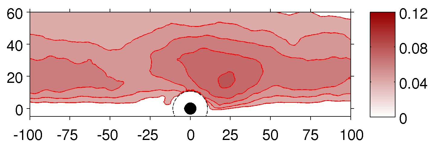
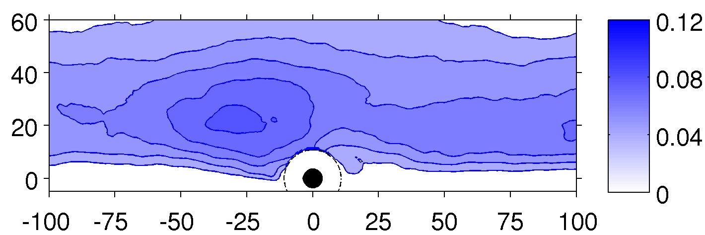
$\tilde{z}^{+}$

$\quad\tilde{y}^{+}$

$(b)$

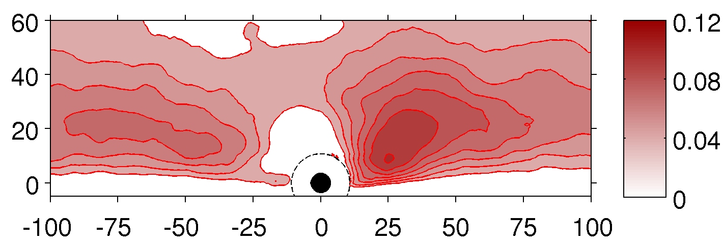
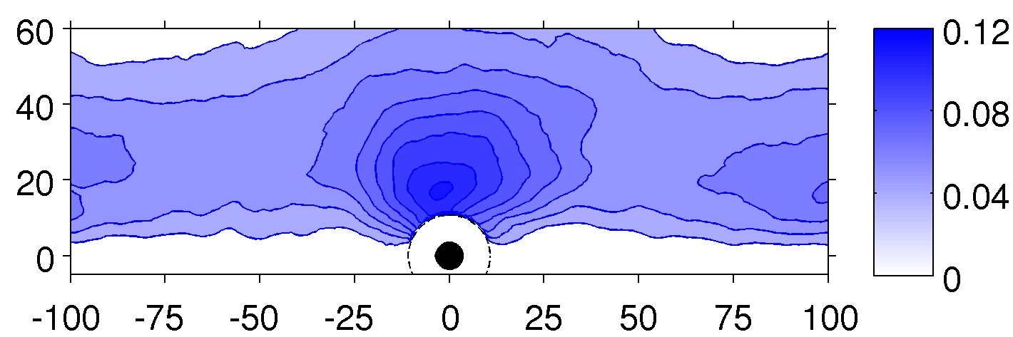
$\tilde{z}^{+}$

$\quad\tilde{y}^{+}$

$(c)$

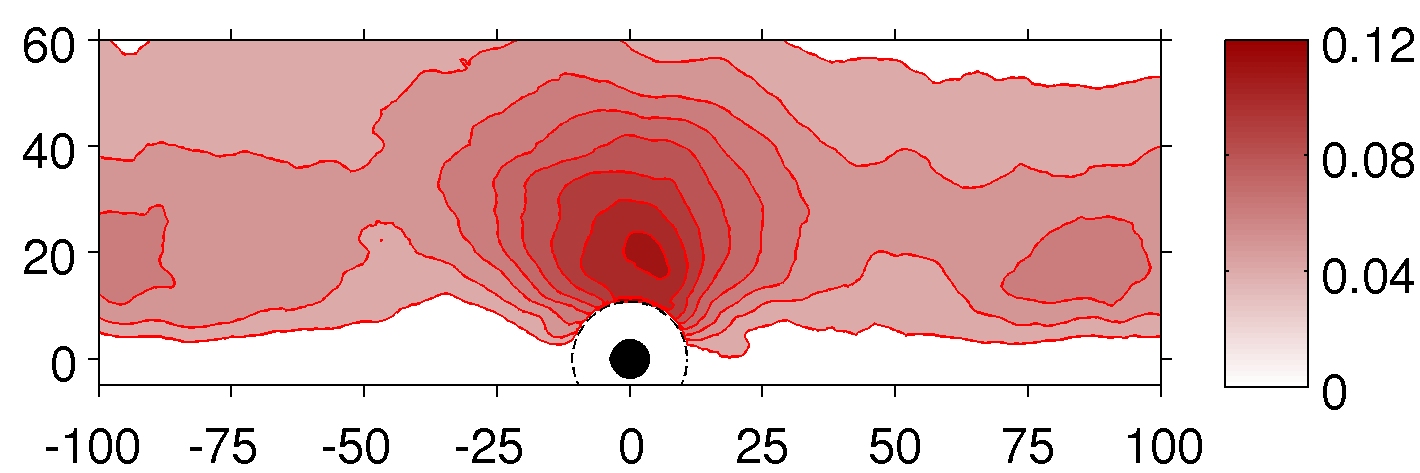
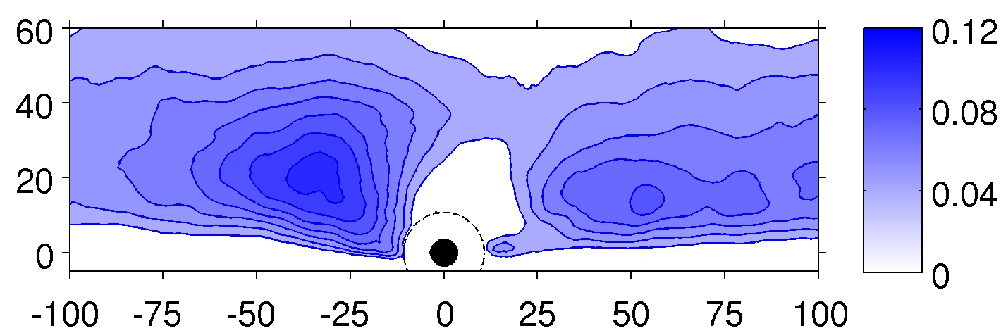
$\tilde{z}^{+}$

$\quad\tilde{y}^{+}$

Figure 24: The spatial distribution of clockwise and counterclockwise rotating vortical regions with respect to the position of a particle in a cross-sectional plane passing through the particle center. The vortical regions are educed from $\tilde{\lambda}_{2}^{\mathrm{\omega_{x}+}}$ (red-colored contours) and $\tilde{\lambda}_{2}^{\mathrm{\omega_{x}-}}$ (blue-colored contours) as defined in (15). (a) shows the probability distribution conditioned to all particles whose centers are located within one particle diameter from the bottom wall. (b) shows the same quantity as in (a) but additionally selecting only particles with positive spanwise velocity $w_{\mathrm{p}}>0$. (c) shows the same quantity as in (a) but additionally selecting only particles with negative spanwise velocity $w_{\mathrm{p}}<0$. Note that the positive $x$-direction points into the paper.

3.6 The role of the streamwise vortices on the distribution of particles

Visual and quantitative evidence provided so far shows that, consistent with previous experimental findings, particles are inhomogeneously distributed at the bottom wall. This results on the one hand in regions of high particle concentrations where particles are observed to form streamwise elongated clusters and on the other hand in void regions of very low particle concentration. It has been shown that particles tend to avoid the high-speed fluid regions and are on average residing in the low-speed fluid regions. As mentioned in the introduction, the behaviour of particle segregation at the bottom wall is believed to be linked to the dynamics of the quasi-streamwise vortices in the near-wall region. These coherent vortical structures are well known to dominate the buffer region in boundary-layer-type flows and are responsible for most of the turbulence activity therein (Robinson, 1991; Jiménez and Pinelli, 1999; Adrian et al., 2000; Schoppa and Hussain, 2000; Adrian, 2007).

With the aim to further analyze the role of the streamwise vortices with respect to particle segregation, we determine the correlation between particle positions and the position of vortical regions in their vicinity. For the identification of vortical regions we have adopted the definition of vortical structures proposed by Jeong and Hussain (1995). A vortex is defined as a region where the second largest eigenvalue $\lambda_{2}$ of the tensor $\mathbf{S}^{2}+\boldsymbol{\Omega}^{2}$ is negative, $\mathbf{S}$ and $\boldsymbol{\Omega}$ being the symmetric and antisymmetric parts of the fluid velocity gradient tensor $\nabla\mathbf{u}_{\mathrm{f}}$. It is well known that in the buffer region of wall-bounded flows, where the quasi-streamwise vortices are dominant, the streamwise vorticity field $\omega_{\mathrm{f,x}}=\partial_{\mathrm{y}}w_{\mathrm{f}}-\partial_{\mathrm{z}}v_{\mathrm{f}}$ is highly correlated with the vortical regions, (Kim et al., 1987). Here the sign of $\omega_{\mathrm{f,x}}$ (positive/negative) is used to determine the sense of rotation (clockwise/counterclockwise) of the vortices educed by means of $\lambda_{2}$. Therefore, we define two real-valued fields $\lambda_{2}^{\mathrm{\omega_{x}+}}$ and $\lambda_{2}^{\mathrm{\omega_{x}-}}$ which indicate whether a given point lies inside a vortical region with, respectively, clockwise or counterclockwise rotation around the streamwise axis, having the amplitude $|\lambda_{2}(\mathbf{x},t)|$, viz.

$$\lambda_{2}^{\mathrm{\omega_{x}+}}(\mathbf{x},t)=\left\{\begin{array}[]{ll}\phi_{\mathrm{f}}(\mathbf{x},t)|\lambda_{2}(\mathbf{x},t)|&\mbox{if}\,\lambda_{2}(\mathbf{x},t)<0,\;\omega_{\mathrm{f,x}}(\mathbf{x},t)>0\\ 0&\mbox{else}\;,\\ \end{array}\right.$$ (14c)

$$\lambda_{2}^{\mathrm{\omega_{x}-}}(\mathbf{x},t)=\left\{\begin{array}[]{ll}\phi_{\mathrm{f}}(\mathbf{x},t)|\lambda_{2}(\mathbf{x},t)|&\mbox{if}\,\lambda_{2}(\mathbf{x},t)<0,\;,\omega_{\mathrm{f,x}}(\mathbf{x},t)<0\\ 0&\mbox{else}\;.\end{array}\right.$$ (14f)

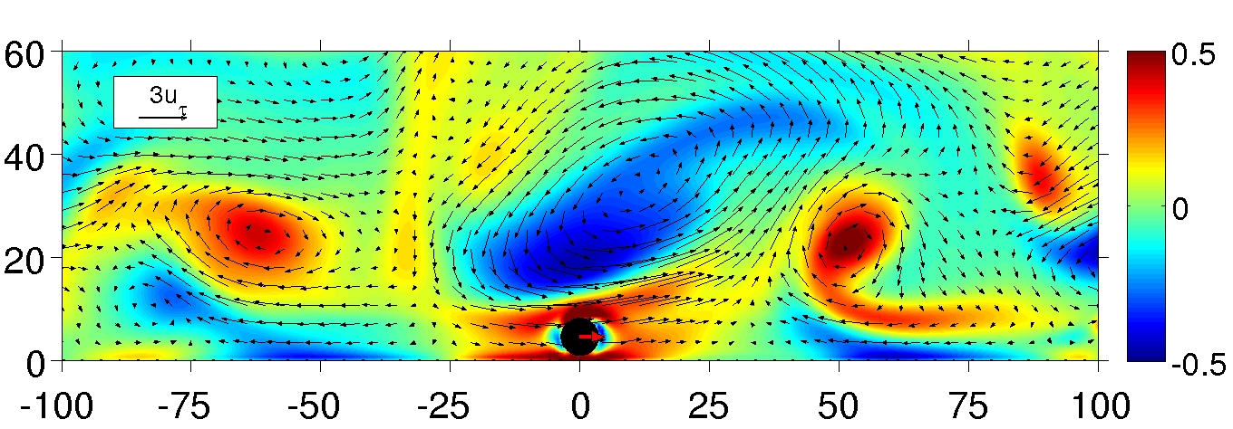
$\tilde{z}^{+}$

$\quad y^{+}$

Figure 25: An instantaneous fluid velocity field (indicated by black arrows) around a particle in spanwise motion (red arrow) in a cross-sectional plane. The background color indicates the streamwise vorticity normalized in wall units, i.e. $\omega_{\mathrm{f,x}}^{+}$. The graph shows only a small part of the entire plane, and the fluid velocity vectors have only been plotted at every 5th grid point in both coordinate directions.

The presence of the fluid indicator function $\phi_{\mathrm{f}}$ in the above definition guarantees that only points in the fluid region are selected. Note that we have additionally excluded a spherical region with radius $3R$ around each particle center in order to consider only the part of the fluid domain $\Omega_{\mathrm{f}}(t)$ which is not directly affected by the particle’s own near-field (cf. § 3.2). Analogous to the notation in previous sections, the fields defined in (14) conditioned upon the $l$th particle are denoted as $\lambda_{2}^{\mathrm{\omega_{x}+},(l)}(\tilde{\mathbf{x}}^{(l)},t)$ and $\lambda_{2}^{\mathrm{\omega_{x}-},(l)}(\tilde{\mathbf{x}}^{(l)},t)$. The average of the quantities $\lambda_{2}^{\mathrm{\omega_{x}+},(l)}$ and $\lambda_{2}^{\mathrm{\omega_{x}-},(l)}$ over all particles and time (as in 10) is denoted as

$$\tilde{\lambda}_{2}^{\mathrm{\omega_{x}+}}(\tilde{\mathbf{x}},y^{(s)})=\langle\lambda_{2}^{\mathrm{\omega_{x}+},(l)}(\tilde{\mathbf{x}}^{(l)},t)\rangle_{\mathrm{p,t}}\;,$$ (15a)

$$\tilde{\lambda}_{2}^{\mathrm{\omega_{x}-}}(\tilde{\mathbf{x}},y^{(s)})=\langle\lambda_{2}^{\mathrm{\omega_{x}-},(l)}(\tilde{\mathbf{x}}^{(l)},t)\rangle_{\mathrm{p,t}}\;.$$ (15b)

The fields $\tilde{\lambda}_{2}^{\mathrm{\omega_{x}+}}$ and $\tilde{\lambda}_{2}^{\mathrm{\omega_{x}-}}$ correspond to averages of the magnitude of (negative-valued) $\lambda_{2}$, conditioned to particle centers located in the wall-normal slab $s$, further distinguishing between positive and negative streamwise rotation of the fluid. Therefore, they give an indication of the intensity of vortical structures (with the respective sense of streamwise rotation) on average found at a given position with respect to a particle.

Figure 24$(a)$ shows the two fields defined in (15) in a cross-sectional plane through the center of the reference particle, selecting by the choice of the slab $s$ those particles with $y_{\mathrm{p}}\leq D$. The two graphs clearly show that those particles are on average found at spanwise positions in between strong vortical regions of opposite sign. The signatures of these prominent counter-rotating vortical regions visible in figure 24$(a)$ are located at wall-normal distances of roughly $\tilde{y}^{+}=20$ to $30$ measured from the reference particle center. The sense of streamwise rotation of the two intense vortical regions is such that a region of low streamwise velocity is induced at around the particle location, in agreement with the results of § 3.4. This result is also consistent with the common occurrence of streamwise vortices flanking low-speed velocity streaks with a positive or negative spanwise shift according to their sign.

In order to analyze the correlation between lateral particle motion and the presence of coherent structures, we have further conditioned the fields defined in (14) with respect to the sign of the spanwise particle velocity $w_{\mathrm{p}}$. The result is shown in figure 24$(b)$ and 24$(c)$ for positive and negative values of $w_{\mathrm{p}}$, respectively. The first observation from these figures is that the condition on the sign of spanwise particle velocity is statistically relevant since the resulting fields are clearly distinct from those in figure 24$(a)$. Most prominently, we find regions of large values of $\tilde{\lambda}_{2}^{\mathrm{\omega_{x}-}}$ ($\tilde{\lambda}_{2}^{\mathrm{\omega_{x}+}}$) directly above particles for which $w_{\mathrm{p}}>0$ ($w_{\mathrm{p}}<0$). The oppositely signed fields ($\tilde{\lambda}_{2}^{\mathrm{\omega_{x}+}}$ in case of $w_{\mathrm{p}}>0$, and $\tilde{\lambda}_{2}^{\mathrm{\omega_{x}-}}$ for $w_{\mathrm{p}}<0$) do not exhibit large values in the direct vicinity of the reference particle. These results confirm that the spanwise motion of near-wall particles is statistically correlated with coherent vortices found in the buffer layer. The data suggests that the lateral particle migration towards the low-speed region is indeed a result of the velocity field induced by the quasi-streamwise vortices.

An example of a particle located below a counter-clockwise rotating vortex and migrating in the positive spanwise direction can be found in figure 25. This particle is immersed in the boundary layer induced by the streamwise vortex immediately located above the particle (around $\tilde{y}^{+}\approx 20$, $\tilde{z}^{+}\approx 0$). The direction of the depicted particle’s spanwise motion is clearly towards the location where an ejection of low-momentum fluid takes place at that instant ($\tilde{z}^{+}\approx 30$ in the figure), i.e. a low-velocity region. The scenario which is captured in figure 25 is representative of many events involving near-bottom particles and quasi-streamwise vortices which we have observed in our data-base.

4 Conclusion

In the present study we have investigated the motion of heavy spherical particles in horizontal open channel flow by means of DNS. The particles are larger than the viscous length scale of the near-wall region, requiring full resolution of the flow in their near-field. The gravitational acceleration was chosen such that the overwhelming part of the particles is residing near the wall-plane. Since the global solid volume fraction in the considered case is very low ($5\cdot 10^{-4}$), the maximum of the average particle concentration obtained near the wall is still comparatively low. The particle-to-fluid density ratio is moderate, leading to a value of the Stokes number based on the viscous time scale which is larger than (but of the same order as) unity.

We have found that the basic statistics of the present fluid velocity field are essentially the same as those of single-phase flow at the same Reynolds number. The two-point correlation of the fluid velocity field, however, is somewhat modified, exhibiting slightly larger correlation lengths in the near-wall region where the bulk of the particles are located.

Concerning the dispersed phase, the mean particle velocity is found to be smaller than the mean fluid velocity at all wall distances. In previous investigations (Kaftori et al., 1995b; Kiger and Pan, 2002) an explanation of this apparent velocity lag based upon preferential particle concentration has already been proposed. However, its confirmation hinges on technical points such as the definition of a relative inter-phase velocity and the performance of particle-conditioned averaging. Therefore, we have investigated the origin of this apparent velocity lag in more detail. For this purpose we have first proposed a method to determine a characteristic fluid velocity in the vicinity of a particle (i.e. the fluid velocity “seen” by the particle) for the case of finite particle sizes. Our definition is based on an average of the fluid velocity over a spherical surface (with radius $R_{s}$) centered at the particle center. The validity of this definition was tested in the case of a single fixed sphere in uniform flow which also allowed us to calibrate the value of $R_{s}$, henceforth set to three times the particle radius. Subsequently, our definition of fluid velocity “seen” by the particles was applied to the present horizontal channel flow data. It was found that the two phases are instantaneously much closer to equilibrium than indicated by the apparent velocity lag, as already observed by previous authors in similar cases (Kaftori et al., 1995b; Kiger and Pan, 2002), albeit using less precise measures of the relative velocity.

We have analyzed the spatial distribution of near-wall particles by means of Voronoi tesselation in a wall-parallel plane. The analysis shows that particles near the wall are strongly accumulating into streamwise elongated structures. From the particle conditioned local volumetric concentration field (closely related to the pairwise distribution function) we deduce that these accumulation regions are of a very large scale, with their streamwise extent of the order of the current domain size and a spanwise repeating pattern over distances of approximately $120$ wall units. The auto-correlation of Voronoi cell areas was found to decay very slowly (Taylor microscale of $5.1$ bulk time units), which indicates that the particle accumulation regions are extremely stable in time. In fact, their time scale is much larger than the time scale deduced from the auto-correlation of particle velocities (the Taylor microscale of the streamwise component measures $1.4$ bulk time units).

Furthermore, we have computed the particle-conditioned fluid velocity field (for near-wall particles) in a coordinate system relative to the particle centers. The average relative velocity is found to exhibit spanwise alternating ridges and troughs (approximately $50$ wall units apart) which are also essentially spanning the entire streamwise domain size. The principal minimum of the average relative velocity is centered upon the reference particle, confirming previous observations that the particles are preferentially residing inside the low-speed streaks of the buffer layer.

Finally, we have performed a vortex eduction study (based upon the $\lambda_{2}$ criterion of Jeong and Hussain, 1995) with the purpose of elucidating the role of coherent structures upon the spanwise motion of particles located near the wall. The particle-conditioned average of the negative part of the $\lambda_{2}$ field (distinguishing between positive and negative values of the streamwise vorticity) clearly shows that near-wall particles are preferentially located at spanwise positions in between and beneath counter-rotating vortical regions, their sense of rotation being consistent with the quasi-streamwise vortices which are known to flank the typical low-speed streaks in the buffer region. When the above particle-conditioned $\lambda_{2}$ field is additionally conditioned upon the spanwise particle velocity, it is observed that the direction of spanwise particle motion is strongly correlated with the presence of a strong vortical region found directly above the reference particle location. The sign of the streamwise vorticity associated with the vortical region found on average above the particles is such that the induced velocity at the particle location is consistent with the sign of the spanwise particle velocity. This result suggests that the spanwise particle motion near the wall is indeed caused by the quasi-streamwise vortices in the buffer layer.

The present study opens several new perspectives. The proposed method to determine a fluid velocity “seen” by the particles appears potentially suitable for the investigation of fluid-particle interaction in a wide range of flow configurations. It has the advantage of being free from an a priori bias towards a specific spatial direction. At the same time the definition can be readily evaluated with the aid of flow data generated by means of interface-resolved direct numerical simulation, or, possibly, data obtained through high-resolution volumetric measurements at the particle scale.

Concerning the interaction of near-wall turbulence and particles in the present case, the dynamical mechanism leading to the formation (and sustenance) of particle accumulation regions in low-speed streaks merits further investigation. In order to provide a “cleaner” and more tractable approach to the numerical simulation of such interaction mechanisms it appears beneficial to consider instead of full turbulence in relatively large domains a smaller “laboratory flow”. This can be achieved either by turning to turbulent flow in smaller domain sizes, i.e. the minimal flow unit of Jiménez and Moin (1991), or, alternatively, to invariant solutions of the Navier-Stokes equations (Kawahara et al., 2012). These alternatives will be considered in future studies.

The data presented in this work can be found at the following URL: http://www.ifh.kit.edu/dns_data.

Appendix A Statistical convergence of the fluid phase data

$\langle\tau\rangle^{*}/(\rho_{\mathrm{f}}u_{\tau}^{2})$

$\quad y/h$

Figure 26: Wall-normal profile of the plane- and time-averaged total shear stress as defined in (17). The dashed line indicates the function $(1-y/h)$.

Fully developed single phase channel flows are characterized by a linear variation as a function of the wall-distance of the plane- and time-averaged total shear stress $\langle\tau\rangle/\rho_{\mathrm{f}}\equiv\nu\partial_{\mathrm{y}}\langle u\rangle-\langle u^{\prime}v^{\prime}\rangle$. Traditionally this linearity critereon is used to check the convergence of statistics. However, in particulate channel flows, particles contribute additional terms to the streamwise momentum balance modifying the total shear stress $\langle\tau\rangle$. In the context of the immersed boundary method, the modified Navier-Stokes equations are solved throughout the entire domain while adding an appropriate volume force term $\mathbf{f}$ to the equations, which imposes the no-slip condition at the location of the particles viz.

$$\left.\begin{array}[]{lll}\partial_{\mathrm{t}}\mathbf{u}+(\mathbf{u}\cdot\nabla)\mathbf{u}+\nabla p&=&\nu\nabla^{2}\mathbf{u}+\mathbf{f}\\[5.0pt] \nabla\cdot\mathbf{u}&=&0\end{array}\right]\quad\mathbf{x}\in\Omega\,,$$ (16)

where $\mathbf{u}=(u,v,w)^{T}$ is the vector of fluid velocities (without distinction between the regions occupied by the fluid and the solid), $p$ is the pressure normalized with the fluid density and $\mathbf{f}=(f_{\mathrm{x}},f_{\mathrm{y}},f_{\mathrm{z}})^{T}$ is the localized volume force term. Integrating the streamwise momentum equation over wall-parallel planes and in time (supposing statistical stationarity), and additionally integrating in the wall-normal direction (from the wall plane $y^{\prime}=0$ up to an undetermined distance $y^{\prime}=y$) yields the following equation:

$$\underbrace{\langle\tau\rangle/\rho_{\mathrm{f}}+\int_{0}^{y}{\langle f_{\mathrm{x}}\rangle}dy^{\prime}}_{\langle\tau\rangle^{*}}=u_{\tau}^{2}\Big{(}1-\frac{y}{h}\Big{)}.$$ (17)

It can be seen from (17) that there is indeed an additional contribution to the momentum balance due to the particle-related forcing term. Thus the modified total shear stress $\langle\tau\rangle^{*}$ should vary linearly for a fully developed particle laden channel flow. Figure 26 shows the wall-normal profile of $\langle\tau\rangle^{*}$ for the fluid statistics accumulated excluding the transient period. The near perfect match with the linear profile indicates that the flow is in a statistically steady state in the considered interval.

Appendix B Averaging operations

B.1 Wall-parallel plane and time averaging

Let us first define an indicator function $\phi_{\mathrm{f}}(\mathbf{x},t)$ for the fluid phase which tells us whether a given point with a position vector $\mathbf{x}$ lies inside $\Omega_{\mathrm{f}}(t)$, the part of the computational domain $\Omega$ which is occupied by fluid at time $t$, as follows:

$$\phi_{\mathrm{f}}(\mathbf{x},t)=\left\{\begin{array}[]{lll}1&\mbox{if}&\mathbf{x}\in\Omega_{\mathrm{f}}(t)\\ 0&\mbox{else}&\end{array}\right.\,.$$ (18)

Furthermore, a discrete counter of fluid sample points in a wall-parallel plane at a given wall-distance $y_{j}$ is defined as:

$$n(y_{j})=\sum_{m=1}^{N_{\mathrm{t}}}\sum_{i=1}^{N_{\mathrm{x}}}\sum_{k=1}^{N_{\mathrm{z}}}\phi_{\mathrm{f}}(\mathbf{x}_{ijk},t^{m})\,,$$ (19)

where $N_{\mathrm{x}}$ and $N_{\mathrm{z}}$ are the number of grid nodes in the streamwise and spanwise directions, $N_{\mathrm{t}}$ is the number of time records in the data set, and a discrete grid position is denoted as $\mathbf{x}_{ijk}=(x_{i},y_{j},z_{k})^{T}$. Consequently, the ensemble average of an Eulerian quantity $\boldsymbol{\xi}_{\mathrm{f}}$ of the fluid phase over wall-parallel planes and in time, while considering only grid points located in the fluid domain, is defined as:

$$\langle\boldsymbol{\xi}_{\mathrm{f}}\rangle(y_{j})=\frac{1}{n(y_{j})}\sum_{m=1}^{N_{\mathrm{t}}}\sum_{i=1}^{N_{\mathrm{x}}}\sum_{k=1}^{N_{\mathrm{z}}}\phi_{\mathrm{f}}(\mathbf{x}_{ijk},t^{m})\,\boldsymbol{\xi}_{\mathrm{f}}(\mathbf{x}_{ijk},t^{m})\,.$$ (20)

In the present study wall-parallel plane averaging of Eulerian quantities was performed during runtime from a total of $N_{\mathrm{t}}=26700$ flow field snapshots.

B.2 Instantaneous box averaging

A global counter of samples in the fluid domain can be defined analogously to (19), viz.

$$n_{xyz}(t)=\sum_{i=1}^{N_{\mathrm{x}}}\sum_{j=1}^{N_{\mathrm{y}}}\sum_{k=1}^{N_{\mathrm{z}}}\phi_{\mathrm{f}}(\mathbf{x}_{ijk},t)\,,$$ (21)

where $N_{\mathrm{y}}$ is the number of grid nodes in the wall-normal direction. The instantaneous average of a quantity $\boldsymbol{\xi}_{\mathrm{f}}$ over the entire volume $\Omega_{f}$ occupied by the fluid is then defined as follows:

$$\langle\boldsymbol{\xi}_{\mathrm{f}}\rangle_{\mathrm{xyz}}(t)=\frac{1}{n_{xyz}(t)}\sum_{i=1}^{N_{\mathrm{x}}}\sum_{j=1}^{N_{\mathrm{y}}}\sum_{k=1}^{N_{\mathrm{z}}}\phi_{\mathrm{f}}(\mathbf{x}_{ijk},t)\,\boldsymbol{\xi}_{\mathrm{f}}(\mathbf{x}_{ijk},t)\,.$$ (22)

B.3 Binned averages over particle-related quantities

Concerning Lagrangian quantities related to particles, the domain was decomposed into discrete wall-parallel bins of thickness $\Delta h$ and averaging was performed over all those particles within each bin. Similar to (18), we define an indicator function $\phi_{\mathrm{bin}}^{(j)}(y)$ which tells us whether a given wall-normal position $y$ is located inside or outside a particular bin with index $j$, viz.

$$\phi_{\mathrm{bin}}^{(j)}(y)=\left\{\begin{array}[]{lll}1&\mbox{if}&(j-1)\Delta h\leq y<j\Delta h\\ 0&\mbox{else}&\end{array}\right.$$ (23)

as well as a sample counter for each bin viz.

$$n_{\mathrm{p}}^{(j)}=\sum_{m=1}^{N_{\mathrm{t}}^{\mathrm{(p)}}}\sum_{l=1}^{N_{\mathrm{p}}}\phi_{\mathrm{bin}}^{(j)}(y_{\mathrm{p}}^{(l)}(t^{m}))\,\,,$$ (24)

where $N_{\mathrm{t}}^{\mathrm{(p)}}$ is the number of available snapshots of the solid phase. From the sample counter we can deduce the average solid volume fraction in each bin, viz.

$$\langle\phi_{s}\rangle(y^{(j)})=\frac{n_{p}^{(j)}}{N_{\mathrm{t}}^{\mathrm{(p)}}}\,\frac{\pi D^{3}}{6L_{x}L_{z}\Delta h}\,.$$ (25)

Finally, the binned average (over time and the number of particles) of a Lagrangian quantity $\boldsymbol{\xi}_{\mathrm{p}}$ is defined as follows:

$$\langle\boldsymbol{\xi}_{\mathrm{p}}\rangle(y^{(j)})=\frac{1}{n_{\mathrm{p}}^{(j)}}\sum_{m=1}^{N_{\mathrm{t}}^{\mathrm{(p)}}}\sum_{l=1}^{N_{\mathrm{p}}}\phi_{\mathrm{bin}}^{(j)}(y_{\mathrm{p}}^{(l)}(t^{m}))\,\boldsymbol{\xi}_{\mathrm{p}}^{(l)}(t^{m})\,,$$ (26)

supposing that a finite number of samples has been encountered ($n_{\mathrm{p}}^{(j)}>0$). Accumulated data related to Lagrangian quantities amounts to a total of $N_{\mathrm{t}}^{\mathrm{(p)}}=20314$ particle fields (more than $10^{7}$ particle samples). A bin thickness of $\Delta h=D/2$ was adopted to evaluate the bin-averages unless otherwise stated. The distribution of samples can be deduced from figure 4 which shows the wall-normal profile of the average solid volume fraction.

B.4 Particle-centered averaging

For performing the particle-conditioned averaging of a field $\boldsymbol{\xi}_{\mathrm{f}}(\mathbf{x},t)$, an averaging volume is considered such that the coordinate system within the volume is defined relative to the center of each of the considered particles. Applying the indicator functions defined above, we define a discrete counter field $\tilde{n}^{(s)}(\tilde{\mathbf{x}}_{ijk})$ which holds the number of samples obtained through averaging at a given discrete location with indices $i,j,k$ for a given $y$-slab with index $s$, viz.

$$\tilde{n}^{(s)}(\tilde{\mathbf{x}}_{ijk})=\sum_{m=1}^{N_{\mathrm{t}}^{\mathrm{(r)}}}\sum_{l=1}^{N_{\mathrm{p}}}\phi_{\mathrm{bin}}^{(s)}(y_{\mathrm{p}}^{(l)}(t^{m}))\,\phi_{\mathrm{f}}(\tilde{\mathbf{x}}_{ijk}^{(l)}(t^{m}),t^{m})\,,$$ (27)

In equation (27) the symbol $t^{m}$ indicates the time corresponding to the $m$th snapshot in the database (comprising a total of $N_{\mathrm{t}}^{\mathrm{(r)}}$ snapshots) and $\tilde{\mathbf{x}}_{ijk}^{(l)}(t^{m})$ is a discrete coordinate relative to the $l$th particle’s center position at time $t^{m}$, as defined in (9). The average of the quantity $\boldsymbol{\xi}_{\mathrm{f}}$ over time and over all particles located within the given wall-parallel slab is then defined as follows:

$$\langle\boldsymbol{\xi}_{\mathrm{f}}\rangle_{\mathrm{p,t}}(\tilde{\mathbf{x}}_{ijk},y^{(s)})=\frac{1}{\tilde{n}^{(s)}(\tilde{\mathbf{x}}_{ijk})}\sum_{m=1}^{N_{\mathrm{t}}^{\mathrm{(r)}}}\sum_{l=1}^{N_{\mathrm{p}}} \phi_{\mathrm{bin}}^{(s)}(y_{\mathrm{p}}^{(l)}(t^{m}))\,\phi_{\mathrm{f}}(\tilde{\mathbf{x}}_{ijk}^{(l)}(t^{m}),t^{m})$$ (28)

$$\times\,\boldsymbol{\xi}_{\mathrm{f}}(\tilde{\mathbf{x}}_{ijk}^{(l)}(t^{m}),t^{m})\,$$

Note that the coordinates $\tilde{\mathbf{x}}_{ijk}^{(l)}(t^{m})$ do not necessarily coincide with the fixed grid used in the direct numerical simulation. Thus, values of $\boldsymbol{\xi}_{\mathrm{f}}$ at $\tilde{\mathbf{x}}_{ijk}^{(l)}(t^{m})$ are determined by a tri-linear interpolation from those values at the neighbouring fixed grid locations.

For evaluating the average defined by (28) a total amount of $N_{\mathrm{t}}^{\mathrm{(r)}}=70$ flow field snapshots evenly distributed in the considered observation interval were used.

References

- Sumer and Oğuz (1978) B. Mutlu Sumer and Beyhan Oğuz. Particle motions near the bottom in turbulent flow in an open channel. J. Fluid Mech., 86:109–127, 1978.
- Yung et al. (1989) B. P. K. Yung, H. Merry, and T. R. Bott. The role of turbulent bursts in particle re-entrainment in aqueous systems. Chem. Eng. Sci., 44:873–882, 1989.
- Rashidi et al. (1990) M. Rashidi, G. Hetsroni, and S. Banerjee. Particle-turbulence interaction in a boundary layer. Int. J. Multiphase Flow, 16:935 – 949, 1990.
- Kaftori et al. (1995a) D. Kaftori, G. Hetsroni, and S. Banerjee. Particle behaviour in the turbulent boundary layer. I. Motion, deposition, and entrainment. Phys. Fluids, 7(5):1095 – 1107, 1995a.
- Kaftori et al. (1995b) D. Kaftori, G. Hetsroni, and S. Banerjee. Particle behaviour in the turbulent boundary layer. II. Velocity and distribution profiles. Phys. Fluids, 7(5):1107 – 1121, 1995b.
- Niño and García (1996) Y. Niño and M. H. García. Experiments on particle-turbulence interactions in the near-wall region of an open channel flow: implications for sediment transport. J. Fluid Mech., 326:285–319, 1996.
- Kiger and Pan (2002) K T Kiger and C Pan. Suspension and turbulence modification effects of solid particulates on a horizontal turbulent channel flow. J. Turb., 3(019):1–17, 2002.
- Righetti and Romano (2004) M. Righetti and G. P. Romano. Particle-fluid interactions in a plane near-wall turbulent flow. J. Fluid Mech., 505:93 – 121, 2004.
- Hetsroni and Rozenblit (1994) G. Hetsroni and R. Rozenblit. Heat transfer to a liquid-solid mixture in a flume. Int. J. Multiphase Flow, 20:671–689, 1994.
- Rouson and Eaton (2001) Damian W. I. Rouson and John K. Eaton. On the preferential concentration of solid particles in turbulent channel flow. J. Fluid Mech., 428:149–169, 2001.
- Marchioli and Soldati (2002) Cristian Marchioli and Alfredo Soldati. Mechanisms for particle transfer and segregation in a turbulent boundary layer. J. Fluid Mech., 468:283 – 315, 2002.
- Narayanan et al. (2003) Chidambaram Narayanan, Djamel Lakehal, Lorenzo Botto, and Alfredo Soldati. Mechanisms of particle deposition in a fully developed turbulent open channel flow. Phys. Fluids, 15:1545473, 2003.
- Picciotto et al. (2005) Maurizio Picciotto, Cristian Marchioli, and Alfredo Soldati. Characterization of near-wall accumulation regions for inertial particles in turbulent boundary layers. Phys. Fluids, 17:098101, 2005.
- Soldati and Marchioli (2009) Alfredo Soldati and Cristian Marchioli. Physics and modelling of turbulent particle deposition and entrainment: Review of a systematic study. Int. J. Multiphase Flow, 35:827–839, 2009.
- Pan and Banerjee (1997) Y. Pan and S. Banerjee. Numerical investigation of the effects of large particles on wall-turbulence. Phys. Fluids, 9(12):3786 – 3807, 1997.
- Uhlmann (2008) Markus Uhlmann. Interface-resolved direct numerical simulation of vertical particulate channel flow in the turbulent regime. Phys. Fluids, 20(5):053305, 2008.
- Shao et al. (2012) Xueming Shao, Tenghu Wu, and Zhaosheng Yu. Fully resolved numerical simulation of particle-laden turbulent flow in a horizontal channel at a low reynolds number. J. Fluid Mech., 693:319–344, 2012.
- García-Villalba et al. (2012) M. García-Villalba, A. G. Kidanemariam, and M. Uhlmann. DNS of vertical plane channel flow with finite-size particles: Voronoi analysis, acceleration statistics and particle-conditioned averaging. Int. J. Multiphase Flow, 46:54–74, 2012.
- Kajishima and Takiguchi (2002) Takeo Kajishima and Saotshi Takiguchi. Interaction between particle clusters and particle-induced turbulence. Int. J. Heat Fluid Fl., 23:639–646, 2002.
- Ten Cate et al. (2004) Andreas Ten Cate, Jos J. Derksen, Luis M. Portela, and Harry E. A. Van Den Akker. Fully resolved simulations of colliding monodisperse spheres in forced isotropic turbulence. J. Fluid Mech., 519:233–271, 2004.
- Lucci et al. (2010) Francesco Lucci, Antonino Ferrante, and Said Elghobashi. Modulation of isotropic turbulence by particles of Taylor length-scale size. J. Fluid Mech., 650:5–55, 2010.
- Lucci et al. (2011) Francesco Lucci, Antonino Ferrante, and Said Elghobashi. Is Stokes number an appropriate indicator for turbulence modulation by particles of Taylor length-scale size. Phys. Fluids, 23:025101, 2011.
- Monchaux et al. (2010) R. Monchaux, M. Bourgoin, and A. Cartellier. Preferential concentration of heavy particles: A vorono analysis. Phys. Fluids, 22:103304, 2010.
- Monchaux et al. (2012) R. Monchaux, M. Bourgoin, and A. Cartellier. Analyzing preferential concentration and clustering of intertial particles in turbulence. Int. J. Multiphase Flow, 40:1–18, 2012.
- Bagchi and Balachandar (2003) P. Bagchi and S. Balachandar. Effect of turbulence on the drag and lift of a particle. Phys. Fluids, 15:3496, 2003.
- Merle et al. (2005) Axel Merle, Dominique Legendre, and Jacques Magnaudet. Forces on a high-Reynolds-number spherical bubble in a turbulent flow. J. Fluid Mech., 532:53–62, 2005.
- Zeng et al. (2008) Lanying Zeng, S. Balachandar, Paul Fischer, and Fady Najjar. Interactions of a stationary finite-sized particle with wall turbulence. J. Fluid Mech., 594:271–305, 2008.
- Uhlmann (2005a) Markus Uhlmann. An immersed boundary method with direct forcing for the simulation of particulate flows. J. Comput. Phys., 209:448 – 476, 2005a.
- Verzicco and Orlandi (1996) R. Verzicco and P. Orlandi. A finite-difference scheme for three-dimensional incompressible flows in cylindrical coordinates. J. Comput. Phys., 123:402–414, 1996.
- Peskin (2002) Charles S. Peskin. The immersed boundary method. In Acta Numerica, volume 11, pages 479 – 517. Cambridge University Press, 2002.
- Glowinski et al. (1999) R. Glowinski, T. W. Pan, T. I. Hesla, and D. D. Joseph. A distributed lagrange multiplier/fictitious domain method for particulate flows. Int. J. Multiphase Flow, 25:755, 1999.
- Uhlmann (2010) M. Uhlmann. Hydrodynamic turbulence induced by sedimenting particles. In B. Mohr and W. Frings, editors, Jülich Blue Gene/P Extreme Scaling Workshop 2010, Technical Report FZJ-JSC-IB-2010-03, pages 35–37, 2010.
- Uhlmann (2004) Markus Uhlmann. New results on the simulation of particulate flows. Technical Report 1038, CIEMAT, Madrid, Spain, 2004.
- Uhlmann (2005b) M. Uhlmann. An improved fluid-solid coupling method for DNS of particulate flow on a fixed mesh. In M. Sommerfeld, editor, Proc. 11th Workshop Two-Phase Flow Predictions, Merseburg, Germany, 2005b. Universität Halle. ISBN 3-86010-767-4.
- Uhlmann (2006) M. Uhlmann. Experience with DNS of particulate flow using a variant of the immersed boundary method. In P. Wesseling, E. Oñate, and J. Périaux, editors, Proc. ECCOMAS CFD 2006, Egmond aan Zee, The Netherlands, 2006. TU Delft. ISBN 90-9020970-0.
- Chan-Braun et al. (2011) C. Chan-Braun, M. García-Villalba, and M. Uhlmann. Force and torque acting on particles in a transitionally rough open channel flow. J. Fluid Mech., 684:441–474, 2011. doi: 10.1017/jfm.2011.311.
- Kim et al. (1987) John Kim, Parviz Moin, and Robert Moser. Turbulence statistics in fully developed channel flow at low reynolds number. J. Fluid Mech., 177:133 – 166, 1987.
- Taniere et al. (1997) A Taniere, B Oesterle, and JC Monnier. On the behaviour of solid particles in a horizontal boundary layer with turbulence and saltation effects. Exp. Fluids, 23(6):463–471, DEC 1997. ISSN 0723-4864.
- Muste et al. (2009) M. Muste, K. Yu, I. Fujita, and R. Ettema. Two-phase flow insights into open-channel flows with suspended particles of different densities. Environ. Fluid Mech., 9:161–186, 2009.
- Noguchi and Nezu (2009) K. Noguchi and I. Nezu. Particle-turbulence interaction and local particle concentration in sediment-laden open-channel flows. J. Hydro-env. Res., 3:54–68, 2009.
- Johnson and Patel (1999) T. A. Johnson and V. C. Patel. Flow past a sphere up to a reynolds number of 300. J. Fluid Mech., 378:19–70, 1999.
- Naso and Prosperetti (2010) A. Naso and A. Prosperetti. The interaction between a solid particle and a turbulent flow. New J. Phys., 12(033040), 2010.
- Okabe et al. (1992) Atsuyuki Okabe, Barry Boots, and Kokich Sugihara. Spatial Tessellations: Concepts and Applications of Voronoi Diagrams. Wiley, Chichester, 2nd edition, 1992.
- Ferenc and Néda (2007) Járai-Szabó Ferenc and Zoltán Néda. On the size distribution of poisson voronoi cells. Physica A, 385(2):518 – 526, 2007. ISSN 0378-4371. doi: DOI:10.1016/j.physa.2007.07.063.
- Sundaram and Collins (1997) Shivshankar Sundaram and Lance R. Collins. Collision statistics in an isotropic particle-laden turbulent suspension. Part 1. Direct numerical simulations. J. Fluid Mech., 335:75–109, 1997.
- Shotorban and Balachandar (2006) Babak Shotorban and S. Balachandar. Particle concentration in homogeneous shear turbulence simulated via lagrangian and equilibrium eulerian approaches. Phys. Fluids, 18:065105, 2006.
- Sardina et al. (2012) G. Sardina, P. Schlatter, L. Brandt, F. Picano, and C. M. Casciola. Wall accumulation and spatial localization in particle-laden wall flows. J. Fluid Mech., 699:50–78, 2012.
- Gualtieri et al. (2009) P. Gualtieri, F. Picano, and C. M. Casciola. Anisotropic clustering of inertial particles in homogeneous shear flow. J. Fluid Mech., 629:25–39, 2009.
- Robinson (1991) S. K. Robinson. Coherent motions in the turbulent boundary layer. Annu. Rev. Fluid Mech., 23:601 – 639, 1991.
- Jiménez and Pinelli (1999) Javier Jiménez and Alfredo Pinelli. The autonomous cycle of near-wall turbulence. J. Fluid Mech., 389:335–359, 1999.
- Adrian et al. (2000) R. J. Adrian, C. D. Meinhart, and C. D. Tomkins. Vortex organization in the outer region of the turbulent boundary layer. J. Fluid Mech., 422:1–54, 2000.
- Schoppa and Hussain (2000) Wade Schoppa and Fazle Hussain. Coherent structure dynamics in near-wall turbulence. J. Fluid Dyn. Res., 26:119–139, 2000.
- Adrian (2007) Ronald J. Adrian. Hairpin vortex organization in wall turbulence. Phys. Fluids, 19:041301, 2007.
- Jeong and Hussain (1995) Jinhee Jeong and Fazle Hussain. On the identification of a vortex. J. Fluid Mech., 285:69–94, 1995.
- Jiménez and Moin (1991) J. Jiménez and P. Moin. The minimal flow unit in near-wall turbulence. J. Fluid Mech., 225:213–240, 1991.
- Kawahara et al. (2012) G. Kawahara, M. Uhlmann, and L. van Veen. The significance of simple invariant solutions in turbulent flows. Ann. Rev. Fluid Mech., 44:203–225, 2012.