Quantum metrology with open dynamical systems

Abstract

This paper studies quantum limits to dynamical sensors in the presence of decoherence. A modified purification approach is used to obtain tighter quantum detection and estimation error bounds for optical phase sensing and optomechanical force sensing. When optical loss is present, these bounds are found to obey shot-noise scalings for arbitrary quantum states of light under certain realistic conditions, thus ruling out the possibility of asymptotic Heisenberg error scalings with respect to the average photon flux under those conditions. The proposed bounds are expected to be approachable using current quantum optics technology.

1 Introduction

The laws of quantum mechanics impose fundamental limitations to the accuracy of measurements, and a fundamental question in quantum measurement theory is how such limitations affect precision sensing applications, such as gravitational-wave detection, optical interferometry, and atomic magnetometry and gyroscopy [1, 2]. With the rapid recent advance in quantum optomechanics [3, 4, 5, 6, 7] and atomic [8, 9] technologies, quantum sensing limits have received renewed interest and are expected to play a key role in future precision measurement applications.

Many realistic sensors, such as gravitational-wave detectors, perform continuous measurements of time-varying signals (commonly called waveforms). For such sensors, a quantum Cramér-Rao bound (QCRB) for waveform estimation [10] and a quantum fidelity bound for waveform detection [11] have recently been proved, generalizing earlier seminal results by Helstrom [12]. These bounds are not expected to be tight when decoherence is significant, however, as [10, 11] use a purification approach that does not account for the inaccessibility of the environment. Given the ubiquity of decoherence in quantum experiments, the relevance of the bounds to practical situations may be questioned.

One way to account for decoherence is to employ the concepts of mixed states, effects, and operations [13]. Such an approach has been successful in the study of single-parameter estimation problems [14, 15, 16, 17, 18, 19, 20, 21], but becomes intractable for nontrivial quantum dynamics. To retain the convenience of a pure Hilbert space, here I extend a modified purification approach proposed in [14, 18, 19, 20] and apply it to more general open-system detection and estimation problems beyond the paradigm of single-parameter estimation considered by previous work [14, 15, 16, 17, 18, 19, 20, 21]. In particular, I show that

1. For optical phase detection with loss and vacuum noise, the errors obey lower bounds that scale with the average photon number akin to reduced shot-noise limits, provided that the phase shift or the quantum efficiency is small enough (the precise conditions will be given later). This rules out Heisenberg scaling of the detectable phase shift [22, 23] in the high-number limit under such conditions, as well as any significant enhancement of the error exponent by quantum illumination [24, 25, 26] in the low-efficiency limit with vacuum noise. Similar results exist when the phase is a waveform.

2. The mean-square error for lossy optical phase waveform estimation also observes a limit with shot-noise scaling, which generalizes the single-parameter results in [15, 16, 17, 18, 19, 20] and rules out the kind of quantum-enhanced scalings suggested by [27, 28, 29, 30] in the high-flux limit.

3. A quantum model of optomechanical force sensing can be transformed to an optical phase sensing problem with classical phase shift, such that a unified formalism can treat both problems and produce tighter bounds than the results in [10, 11].

These results not only provide more general and realistic quantum limits that can be approached using current quantum optics technology [31, 32, 33, 34, 35, 36], but may also be relevant to more general studies of quantum metrology and quantum information, such as quantum speed limits [37, 38] and Loschmidt echo [39].

2 The modified purification approach

Let $x$ be the vector of unknown parameters to be estimated and $y$ be the observation. Within the purification approach [10, 11], the dynamics of a quantum sensor is modeled by unitary evolution ($U_{x}$ as a function of $x$) of an initial pure density operator $\rho=|\Psi\rangle\langle\Psi|$, and measurements are modeled by a final-time positive operator-valued measure (POVM) $E(y)$ using the principle of deferred measurement [40]. The likelihood function becomes

$$P(y|x)=\textrm{tr}\left[E(y)U_{x}\rho U_{x}^{\dagger}\right].$$ (1)

For continous-time problems, discrete time is first assumed and the continuous limit is taken at the end of calculations. [10, 11] derive quantum bounds by considering the density operator $U_{x}\rho U_{x}^{\dagger}$.

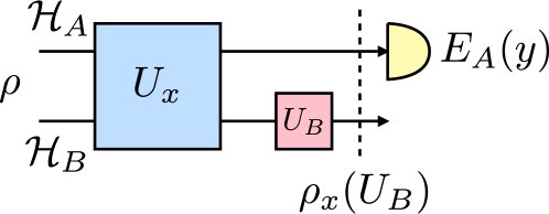
Figure 1: Quantum circuit diagram [40] for the modified purification approach.

Suppose that the Hilbert space ($\mathcal{H}=\mathcal{H}_{A}\otimes\mathcal{H}_{B}$) is divided into an accessible part ($\mathcal{H}_{A}$) and an inaccessible part ($\mathcal{H}_{B}$). The POVM should now be written as $E(y)=E_{A}(y)\otimes 1_{B}$, where $E_{A}(y)$ is a POVM on $\mathcal{H}_{A}$ and $1_{B}$ is the identity operator on $\mathcal{H}_{B}$, which accounts for the fact that $\mathcal{H}_{B}$ cannot be measured. The key to the modified purification approach, as illustrated by Fig. 1, is to recognize that the likelihood function is unchanged if any arbitrary $x$-dependent unitary $U_{B}$ on $\mathcal{H}_{B}$ is applied before the POVM:

$$P(y|x)=\textrm{tr}\left\{\left[E_{A}(y)\otimes 1_{B}\right]\rho_{x}(U_{B})\right\},$$ (2)

where

$$\rho_{x}(U_{B})\equiv(1_{A}\otimes U_{B}^{\dagger})U_{x}\rho U_{x}^{\dagger}(1_{A}\otimes U_{B})$$ (3)

is a purification of $\textrm{tr}_{B}(U_{x}\rho U_{x}^{\dagger})$, such that $\textrm{tr}_{B}\rho_{x}=\textrm{tr}_{B}(U_{x}\rho U_{x}^{\dagger})$. Judicious choices of $U_{B}$ can result in tighter quantum bounds as a function of $\rho_{x}(U_{B})$ [14, 18, 19, 20].

First, suppose that $x^{(0)}$ and $x^{(1)}$ are the two hypotheses for $x$ and $\tilde{x}(y)$ is the estimate. The following theorems are applications of the modified purification and Helstrom’s bounds for pure states [12]:

Theorem 1 (Fidelity bound, Neyman-Pearson criterion).

For any POVM measurement $E_{A}(y)$ of $\textrm{tr}_{B}\rho_{x}$ in $\mathcal{H}_{A}$, the miss probability, defined as

$$P_{01}\equiv\int_{\tilde{x}(y)=x^{(0)}}dyP(y|x^{(1)}),$$ (4)

given a constraint on the false-alarm probability

$$P_{10}\equiv\int_{\tilde{x}(y)=x^{(1)}}dyP(y|x^{(0)})\leq\alpha,$$ (5)

satisfies

$$P_{01}\geq\beta(\alpha,F)\equiv\bigg{\{}\begin{array}[]{ll}1-\left[\sqrt{\alpha F}+\sqrt{(1-\alpha)(1-F)}\right]^{2},&\alpha<F,\\ 0,&\alpha\geq F,\end{array}$$ (8)

where $F$ is the fidelity between the following pure states in $\mathcal{H}_{A}\otimes\mathcal{H}_{B}$:

$$\rho_{0}\equiv U_{B}^{\dagger}U_{0}|\Psi\rangle\langle\Psi|U_{0}^{\dagger}U_{B},$$ (9)

$$\rho_{1}\equiv U_{1}|\Psi\rangle\langle\Psi|U_{1}^{\dagger},$$ (10)

$$F(\rho_{0},\rho_{1})\equiv\left|\langle\Psi|U_{1}^{\dagger}U_{B}^{\dagger}U_{0}|\Psi\rangle\right|^{2},$$ (11)

$\rho_{m}\equiv\rho_{x^{(m)}}$, $U_{m}\equiv U_{x^{(m)}}$, and $1_{A}\otimes U_{B}$, abbreviated as $U_{B}$, is an arbitrary unitary on $\mathcal{H}_{B}$.

Theorem 2 (Fidelity bound, Bayes criterion).

The average error probability $P_{e}\equiv P_{10}P_{0}+P_{01}P_{1}$ with prior probabilities $P_{0}$ and $P_{1}=1-P_{0}$ satisfies

$$P_{e}\geq\frac{1}{2}\left(1-\sqrt{1-4P_{0}P_{1}F}\right)\geq P_{0}P_{1}F.$$ (12)

Proof of Theorem 1 and 2.

[12] shows that the bounds with the likelihood function $P(y|x)=\textrm{tr}[E(y)\rho_{x}]$ are valid for any POVM $E(y)$ on $\mathcal{H}_{A}\otimes\mathcal{H}_{B}$, so they must also be valid with $P(y|x)=\textrm{tr}_{A}[E_{A}(y)\textrm{tr}_{B}\rho_{x}]=\textrm{tr}\{[E_{A}(y)\otimes 1_{B}]\rho_{x}\}$ for any POVM $E_{A}(y)$ on $\mathcal{H}_{A}$. ∎

Since the lower bounds are valid for any $U_{B}$, $U_{B}$ should be chosen to increase $F$ and tighten the bounds. The maximum $F$ becomes the Uhlmann fidelity between mixed states $\textrm{tr}_{B}\rho_{0}$ and $\textrm{tr}_{B}\rho_{1}$ [40, 41]. The bound on $P_{e}$ obtained using this method is thus weaker than the Helstrom bound for the mixed states [12], although it can be shown that the error exponent for the Uhlmann-fidelity bound is within 3dB of the optimal value [42].

Next, consider the estimation of continuous parameters $x$ with prior distribution $P(x)$. A lower error bound is given by the following:

Theorem 3 (Bayesian quantum Cramér-Rao bound).

The error covariance matrix

$$\Sigma\equiv\mathbb{E}\left(\tilde{x}-x\right)\left(\tilde{x}-x\right)^{\top}=\int dydxP(y|x)P(x)\left(\tilde{x}-x\right)\left(\tilde{x}-x\right)^{\top}$$ (13)

satisfies a matrix inequality given by

$$\Sigma\geq\left(J^{(Q)}+J^{(C)}\right)^{-1},$$ (14)

where

$$J_{jk}^{(Q)} =-2\int dxP(x)\frac{\partial^{2}F(\rho_{x},\rho_{x^{\prime}})}{\partial x_{j}^{\prime}\partial x_{k}^{\prime}}\Bigg{|}_{x^{\prime}=x},$$ (15)

$$J_{jk}^{(C)} =\int dxP(x)\frac{\partial\ln P(x)}{\partial x_{j}}\frac{\partial\ln P(x)}{\partial x_{k}}.$$ (16)

Proof.

See [10] for a proof of (14). To relate $J^{(Q)}$ and $F$ as in (15), first note the identity that relates the Bures distance $D_{B}^{2}(\rho_{x},\rho_{x+dx})$ between two density matrices separated by an infinitesimal parameter change to the quantum Fisher information (QFI) matrix $\mathcal{J}^{(Q)}(x)$ [43, 44]:

$$D_{B}^{2}(\rho_{x},\rho_{x+dx})=2\left[1-\sqrt{F(\rho_{x},\rho_{x+dx})}\right]=\frac{1}{4}\sum_{j,k}\mathcal{J}_{jk}^{(Q)}(x)dx_{j}dx_{k}.$$ (17)

This allows one to write the fidelity as

$$F(\rho_{x},\rho_{x+dx})=1-\frac{1}{4}\sum_{j,k}\mathcal{J}_{jk}^{(Q)}(x)dx_{j}dx_{k},$$ (18)

and $\mathcal{J}^{(Q)}(x)$ as

$$\mathcal{J}_{jk}^{(Q)}(x)=-2\frac{\partial^{2}F(\rho_{x},\rho_{x^{\prime}})}{\partial x_{j}^{\prime}\partial x_{k}^{\prime}}\Bigg{|}_{x^{\prime}=x}.$$ (19)

According to [10], the Bayes QFI $J^{(Q)}$ is the average of $\mathcal{J}^{(Q)}(x)$ over the prior probability distribution $P(x)$. (15) then follows. ∎

Here I focus on the Bayes version of the QCRB because the inclusion of prior information is crucial in waveform estimation [10, 45]. The Bayes bound also has the advantage of being applicable to both biased and unbiased estimates [10, 45]. $U_{B}$ should again be chosen to reduce $J^{(Q)}(U_{B})$ and thus tighten the QCRB.

An alternative to the QCRB is a multiparameter form of the quantum Ziv-Zakai bound [46, 47], which can also be expressed in terms of the fidelity, but that option is beyond the scope of this paper.

3 Lossy optical phase detection

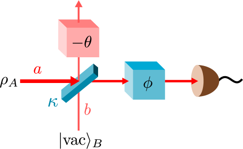
Figure 2: A model of the lossy optical phase sensing problem.

To introduce a new technique of bounding the fidelity, I first consider the simplest setting of an optical phase detection problem, where one optical mode is used to detect a phase shift [22, 23], as depicted in Fig. 2. Let $\phi$ the phase shift between the two hypotheses, $U_{0}=U_{A}U_{AB}$, and $U_{1}=U_{AB}$, where

$$U_{A} =\exp\left(i\phi n\right),\qquad n\equiv a^{\dagger}a,$$ (20)

$$U_{AB} =\exp\left[i\kappa\left(a^{\dagger}b+ab^{\dagger}\right)\right].$$ (21)

$a$ and $b$ are annihilation operators for two different modes that satisfy commutation relations $[a,a^{\dagger}]=[b,b^{\dagger}]=1$, $n$ is the photon-number operator for the $A$ mode, $U_{AB}$ models loss as a beam-splitter coupling with another optical mode $B$ in vacuum state $|0\rangle_{B}$ before the phase modulation, such that $|\Psi\rangle=|\psi\rangle_{A}\otimes|0\rangle_{B}$. $U_{AB}$ can also account for loss after the modulation, as shown in A. The fidelity becomes

$$F=\left|\langle\Psi|U_{AB}^{\dagger}U_{B}^{\dagger}U_{A}U_{AB}|\Psi\rangle\right|^{2}.$$ (22)

Choosing

$$U_{B}=\exp\left(i\theta b^{\dagger}b\right),$$ (23)

where $\theta$ is a free parameter to be specified later, one can simplify (22) using the $SU(2)$ disentangling theorem [48], as shown in B. The result is

$$F =\left|\langle\psi|z^{n}|\psi\rangle\right|^{2},$$ (24)

$$z \equiv\eta e^{i\phi}+(1-\eta)e^{-i\theta},$$ (25)

with

$$\eta\equiv\cos^{2}\kappa$$ (26)

defined as the quantum efficiency. For example, as shown in B, the fidelity for a coherent state is

$$F_{\textrm{coh}} =\exp\left(-4\eta\langle n\rangle\sin^{2}\frac{\phi}{2}\right),$$ (27)

where $\langle O\rangle\equiv\langle\psi|O|\psi\rangle$. Since $-\ln F_{\textrm{coh}}$ depends linearly on the average photon number $\langle n\rangle$, I shall define the linear scaling of $-\ln F$ with respect to $\langle n\rangle$ as the shot-noise scaling for the fidelity. Measurements that can saturate the Bayes error bound in Theorem 2 for coherent states are known [12, 31, 32, 33].

To bound $F$ in general, Jensen’s inequality can be used if $z$ is real and positive. The following lemma provides the necessary and sufficient condition:

Lemma 1.

There exists a $\theta$ such that $z\equiv\eta e^{i\phi}+(1-\eta)e^{-i\theta}$ is real and positive if and only if one of the following conditions is satisfied:

$${\rm(I)} :\ \eta<\frac{1}{2},$$ (28)

$${\rm(II)} :\ \eta\geq\frac{1}{2}{\rm\ and\ }|\sin\phi|\leq\frac{1-\eta}{\eta}{\rm\ and\ }\cos\phi>0.$$ (29)

Proof.

Consider the circle traced by $z(\theta)$ centered at $\eta e^{i\phi}$ with radius $1-\eta$ on the complex plane. $z=|z|>0$ for some $\theta$ is equivalent to the condition that the circle intersects the positive real axis, for which the necessary and sufficient condition is given by one of (28) (the circle encloses the origin for any $\phi$ and thus always intersects the axis) and (29) (the circle intersects the axis for some $\phi$ on the right-hand plane only). ∎

(29) holds when $\phi$ is sufficiently small. For example, $M\sim 100$, $|q|\sim 10^{-19}~{}$m, $2\pi/k\sim 1~{}\mu$m, and $(1-\eta)/\eta\sim 10^{-2}$ for LIGO [49], leading to $|\phi|\sim 2Mk|q|\sim 10^{-10}$, and (29) is easily satisfied.

The following theorem is a key technical result of this paper:

Theorem 4.

If (28) or (29) is satisfied,

$$F \geq F_{z}\equiv z^{2\langle n\rangle},$$ (30)

where

$$z\equiv\eta e^{i\phi}+(1-\eta)e^{-i\theta},$$ (31)

and $\theta$ is chosen to make $z$ real and positive.

Proof.

With $z=|z|>0$ under the condition in Lemma 1 and writing $|\psi\rangle$ as a superposition of eigenstates of $n$, one can apply Jensen’s inequality and obtain $\langle z^{n}\rangle\geq z^{\langle n\rangle}$. (30) then follows from (24). ∎

Compared with the coherent-state value given by (27), $F_{z}$ has the same shot-noise scaling with respect to the average photon number $\langle n\rangle$, as both $-\ln F_{\textrm{coh}}$ and $-\ln F_{z}$ scale linearly with $\langle n\rangle$. Since error-free detection with $F=0$ is possible with pure states [50], this shot-noise-scaling bound is a very strong result. It should also have implications for M-ary phase discrimination in general [51, 52].

The following corollaries are some analytic consequences of Theorem 4 that exemplify its tightness:

Corollary 1.

If $|\phi|\ll 1$ and $|\eta\phi/(1-\eta)|\ll 1$,

$$F_{z} \approx\exp\left[-\frac{\eta}{1-\eta}\langle n\rangle\phi^{2}\right].$$ (32)

Proof.

Let $\theta_{0}\equiv\eta\phi/(1-\eta)$. Since $\textrm{Im}\,z=\eta\sin\phi-(1-\eta)\sin\theta=0$, $\theta=\theta_{0}[1+O(\phi^{2})+O(\theta_{0}^{2})]$, $z^{2}=1-4\eta(1-\eta)\sin^{2}[(\phi+\theta)/2]=1-\theta_{0}\phi[1+O(\phi^{2})+O(\theta_{0}^{2})]$, and $\ln z^{2}=-\theta_{0}\phi[1+O(\theta_{0}\phi)+O(\phi^{2})+O(\theta_{0}^{2})]$, which determines $F_{z}$ in (30) and leads to (32). ∎

(32) differs from $F_{\textrm{coh}}\approx\exp(-\eta\langle n\rangle\phi^{2})$ by just a constant factor of $1/(1-\eta)$ in the exponent. This $1/(1-\eta)$ enhancement factor is the same as the maximum QFI enhancement factor in lossy static-phase estimation [15, 16, 17, 18, 19, 20].

To obtain another measure of detection error, I formalize the concept of detectable phase shift [22, 23] as follows:

Definition 1 (Detectable phase shift).

A detectable phase shift $\phi^{\prime}$ given acceptable error probabilities $\alpha^{\prime}$ and $\beta^{\prime}$ is a $\phi$ that makes $P_{10}\leq\alpha^{\prime}$ and $P_{01}\leq\beta^{\prime}$.

Corollary 2.

Assuming that (32) is an equality,

$$\phi^{\prime 2} \geq\frac{1-\eta}{\eta\langle n\rangle}(-\ln F^{\prime}),$$ (33)

where

$$F^{\prime}\equiv\max_{\beta^{\prime}\geq\beta(\alpha^{\prime},F)}F$$ (34)

and $\beta$ is defined in (8).

Proof.

Any achievable $(P_{10},P_{01})$ must lie above the convex curve $P_{01}=\beta(P_{10},F)$. This means that for $P_{10}\leq\alpha^{\prime}$ and $P_{01}\leq\beta^{\prime}$, $\beta^{\prime}\geq\beta(\alpha^{\prime},F)$ must hold, and hence $F\leq\max_{\beta^{\prime}\geq\beta(\alpha^{\prime},F)}F\equiv F^{\prime}(\alpha^{\prime},\beta^{\prime})$. Since $F\geq F_{z}$, $F_{z}\leq F^{\prime}$ must hold for the constraints on $(P_{10},P_{01})$ to be possible. (33) then follows from (32). ∎

The lower bound in (33) is lower than the shot-noise limit by a constant factor of $1-\eta$ only, ruling out the kind of Heisenberg scaling suggested by [22, 23] for lossy weak phase detection in the $\langle n\rangle\to\infty$ limit.

Corollary 3.

If $\eta\ll 1$, $F_{z}\approx F_{{\rm coh}}$.

Proof.

Since $\textrm{Im}\,z=0$, $\theta=\sin^{-1}[\eta\sin\phi/(1-\eta)]=O(\eta)$, $z=\textrm{Re}\,z=\eta\cos\phi+(1-\eta)\cos\theta=1+\eta\cos\phi-\eta+O(\eta^{2})$, and $\ln z^{2}=-4\eta\sin^{2}(\phi/2)+O(\eta^{2})$, which leads to $-\ln F_{z}=-[1+O(\eta)]\ln F_{\textrm{coh}}$. ∎

Corollary 3 proves that, analogous to the case of target detection [53], the coherent state is near-optimal for any phase detection problem in the low-efficiency limit with vacuum noise, ruling out any significant enhancement of the error exponent by quantum illumination [24, 25, 26]. It remains an open question whether quantum illumination is useful for high-thermal-noise low-efficiency phase detection, as [24, 25] show that quantum illumination is useful for low-efficiency target detection only when the thermal noise is high.

4 Waveform detection

Figure 3: A model of the lossy optical phase waveform sensing problem.

I now turn to the problem of waveform detection, as depicted in Fig. 3. The results are all natural generalizations of the single-mode case. Let $\phi(t)$ be the time-varying phase shift between the two hypotheses, $U_{0}=U_{A}U_{AB}$, and $U_{1}=U_{AB}$, where

$$U_{A} =\exp\left[i\int dt\phi(t)I(t)\right],\qquad I(t)\equiv a^{\dagger}(t)a(t),$$ (35)

$$U_{AB} =\exp\left\{i\kappa\int dt\left[a^{\dagger}(t)b(t)+a(t)b^{\dagger}(t)\right]\right\},\qquad\int dt\equiv\int_{t_{0}}^{t_{f}}dt.$$ (36)

$a(t)$ and $b(t)$ are now annihilation operators for one-dimensional optical fields with commutation relations $[a(t),a^{\dagger}(t^{\prime})]=[b(t),b^{\dagger}(t^{\prime})]=\delta(t-t^{\prime})$ and $I(t)$ is the photon flux [54]. Choosing

$$U_{B}=\exp\left[i\int dt\theta(t)b^{\dagger}(t)b(t)\right],$$ (37)

where $\theta(t)$ is a free function to be specified later, the fidelity can be computed by a discrete-time approach. This is done by deriving the fidelity for the multimode case, writing $a(t_{j})=\sqrt{\delta t}a_{j}$ and $b(t_{j})=\sqrt{\delta t}b_{j}$ in terms of the discrete-mode operators $a_{j}$ and $b_{j}$ and time $t_{j}=t_{0}+j\delta t$, and taking the $\delta t\to 0$ continuous-time limit at the end of the calculations. The result is

$$F[\phi(t)]=\left|\langle\Psi|U_{AB}^{\dagger}U_{B}^{\dagger}U_{A}U_{AB}|\Psi\rangle\right|^{2}=\left|\langle\psi|\exp\left[\int dtI(t)\ln z(t)\right]|\psi\rangle\right|^{2},$$ (38)

$$z(t)\equiv\eta e^{i\phi(t)}+(1-\eta)e^{-i\theta(t)}.$$ (39)

For example, the coherent-state value is

$$F_{\textrm{coh}}[\phi(t)] =\exp\left[-4\eta\int dt\langle I(t)\rangle\sin^{2}\frac{\phi(t)}{2}\right].$$ (40)

$-\ln F_{\textrm{coh}}[\phi(t)]$ scales linearly with $\langle I(t)\rangle$, and this linear scaling shall be defined as the shot-noise scaling for waveform detection.

Jensen’s inequality can again be used to bound the fidelity in (38) if $z(t)$ is real and positive. The generalizations of Theorem 4 and Corollaries 1, 2, and 3 for waveform detection are listed below (with the proofs omitted because they are straightforward generalizations of the ones in the single-mode case):

Corollary 4.

If (28) or (29) is satisfied for all $\phi(t)$,

$$F[\phi(t)]\geq F_{z}[\phi(t)]\equiv\exp\left[\int dt\left\langle I(t)\right\rangle\ln z^{2}(t)\right],$$ (41)

where

$$z(t)\equiv\eta e^{i\phi(t)}+(1-\eta)e^{-i\theta(t)},$$ (42)

and $\theta(t)$ is chosen to make $z(t)$ real and positive.

This bound is also a shot-noise-scaling bound, as $-\ln F_{z}[\phi(t)]$ scales linearly with $\langle I(t)\rangle$.

Corollary 5.

If $|\phi(t)|\ll 1$ and $|\eta\phi(t)/(1-\eta)|\ll 1$,

$$F_{z}[\phi(t)] \approx\exp\left[-\frac{\eta}{1-\eta}\int dt\langle I(t)\rangle\phi^{2}(t)\right].$$ (43)

The enhancement factor $1/(1-\eta)$ in the exponent is the same as that in the single-mode case in (32).

Corollary 6.

Assuming that (43) is an equality, a detectable phase shift $\phi^{\prime}(t)$ satisfies

$$\int dt\langle I(t)\rangle\phi^{\prime 2}(t) \geq\frac{1-\eta}{\eta}(-\ln F^{\prime}),$$ (44)

where $F^{\prime}$ is defined in (34).

(44) is a more general form of the shot-noise limit on a detectable phae shift. For example, if $\langle I(t)\rangle$ is constant, the time-averaged energy of the detectable phase shift satisfies

$$\frac{1}{t_{f}-t_{0}}\int dt\phi^{\prime 2}(t) \geq\frac{1-\eta}{\eta N}(-\ln F^{\prime}),$$ (45)

with $N\equiv(t_{f}-t_{0})\langle I\rangle$.

Corollary 7.

If $\eta\ll 1$, $F_{z}[\phi(t)]\approx F_{{\rm coh}}[\phi(t)]$.

This means that, similar to the single-mode case, the coherent state is near-optimal for phase waveform detection in the low-efficiency limit with vacuum noise, and no significant quantum enhancement is possible even when multiple modes are available.

The derivations so far assume that the waveform $\phi(t)$ is known exactly. Error bounds for stochastic waveform detection can also be obtained by averaging $F[\phi(t)]$ over the prior statistics of $\phi(t)$, as shown in [11], and analytically tractable bounds can be obtained if the prior statistics are Gaussian and $F[\phi(t)]$ is also Gaussian, such as the one given by (43).

5 Waveform estimation

Consider now the waveform estimation problem, using the same model shown in Fig. 3. Unlike the previous section, where the free function $\theta(t)$ is chosen to be an instantaneous function of $\phi(t)$, here I assume $\theta(t)=\int d\tau\lambda(t-\tau)\phi(\tau)$, as this can result in an even tighter but still analytically tractable bound. The QFI $J^{(Q)}(t_{j},t_{k})\equiv\lim_{\delta t\to 0}J_{jk}^{(Q)}/\delta t^{2}$ for estimating $\phi(t)$ is calculated in C and given by

$$J_{\phi}^{(Q)}(t,t^{\prime}) =4\int d\tau d\tau^{\prime}\Big{[}r_{1}(t,\tau)r_{1}(t^{\prime},\tau^{\prime})\left\langle\Delta I(\tau)\Delta I(\tau^{\prime})\right\rangle$$

$$\quad+r_{2}(t,\tau)r_{2}(t^{\prime},\tau^{\prime})\left\langle I(\tau)\right\rangle\delta(\tau-\tau^{\prime})\Big{]},$$

$$r_{1}(t,\tau) \equiv\eta\delta(t-\tau)-(1-\eta)\lambda(\tau-t),$$

$$r_{2}(t,\tau) \equiv\sqrt{\eta(1-\eta)}\left[\delta(t-\tau)+\lambda(\tau-t)\right],$$

$$\Delta I(t) \equiv I(t)-\langle I(t)\rangle.$$ (46)

If the light source has stationary statistics, $\langle I(t)\rangle$ is constant, $\langle\Delta I(t)\Delta I(t^{\prime})\rangle$ depends on $t-t^{\prime}$ only, and a power spectral density $S_{\Delta I}(\omega)$ can be defined by

$$\langle\Delta I(t)\Delta I(t^{\prime})\rangle=\int_{-\infty}^{\infty}\frac{d\omega}{2\pi}S_{\Delta I}(\omega)\exp[i\omega(t-t^{\prime})].$$ (47)

A spectral form of $J_{\phi}^{(Q)}$ in the limit $(t_{0},t_{f})\to(-\infty,\infty)$ is then

$$J_{\phi}^{(Q)}(\omega)=4\left[|\eta-(1-\eta)\lambda(\omega)|^{2}S_{\Delta I}(\omega)+|1+\lambda(\omega)|^{2}\eta(1-\eta)\langle I\rangle\right],$$ (48)

$$\lambda(\omega)\equiv\int dt\lambda(t)\exp(i\omega t).$$ (49)

The minimum QFI becomes

$$\min_{\lambda}J_{\phi}^{(Q)}(\omega)=4\left[\frac{1}{S_{\Delta I}(\omega)}+\frac{1-\eta}{\eta\left\langle I\right\rangle}\right]^{-1}.$$ (50)

This is a generalization of earlier results for lossy static-phase estimation in [15, 16, 17, 18, 19, 20]. Assuming further that $\phi(t)$ is a linear functional of the waveform of interest $x(t)$,

$$\phi(t)=\int dt^{\prime}g(t-t^{\prime})x(t^{\prime}),$$ (51)

a QCRB is then [10]

$$\mathbb{E}[\tilde{x}(t)-x(t)]^{2}\geq\int_{-\infty}^{\infty}\frac{d\omega}{2\pi}\frac{1}{|g(\omega)|^{2}\min_{\lambda}J_{\phi}^{(Q)}(\omega)+J_{x}^{(C)}(\omega)},$$ (52)

where $g(\omega)\equiv\int dtg(t)\exp(i\omega t)$ and $J_{x}^{(C)}(\omega)$ is the prior information in spectral form. For a coherent state,

$$\langle\Delta I(t)\Delta I(t^{\prime})\rangle_{\textrm{coh}}=\langle I\rangle\delta(t-t^{\prime}),$$ (53)

$$S_{\Delta I,\textrm{coh}}(\omega)=\langle I\rangle,$$ (54)

$$\min_{\lambda}J_{\phi,\textrm{coh}}^{(Q)}(\omega)=4\eta\langle I\rangle.$$ (55)

Compared with the coherent-state value, the QFI for any state is limited by the same shot-noise scaling:

$$\min_{\lambda}J_{\phi}^{(Q)}(\omega)\leq\frac{4\eta\langle I\rangle}{1-\eta}.$$ (56)

This rules out the kind of quantum-enhanced scalings suggested by [27, 28, 29, 30] in the high-flux limit when loss is present.

6 Optomechanical force sensing

Figure 4: Schematic of a quantum optomechanical force sensor.

For a more complex example, consider the estimation of a force $x(t)$, $t\in[t_{0},t_{f}]$, on a quantum moving mirror via continuous optical measurements, as illustrated in Fig. 4. For simplicity, assume that any optical cavity dynamics can be adiabatically eliminated [7]. Let $(q,p)$ be the mechanical position and momentum operators, and $a(t)$ be the annihilation operator for the one-dimensional optical field. Suppose

$$U_{x}=U[x(t)]=\mathcal{T}\exp\left[\frac{1}{i\hbar}\int_{t_{0}}^{t_{f}}dtH(t,x(t))\right],$$ (57)

with a Hamiltonian given by

$$H(t,x(t))=H_{B}(t,q,p,x(t))-2\hbar MkqI(t),$$ (58)

where $\mathcal{T}$ is the time-ordering superoperator, $H_{B}$ is the mechanical Hamiltonian, $M$ is the effective number of optical reflections by the mirror, $k$ is the optical wavenumber, and $I(t)\equiv a^{\dagger}(t)a(t)$ is the photon flux.

In an optomechanics experiment, the mechanical oscillator is measured only through the optical field, so one can take the mechanical Hilbert space to be part of the inaccessible Hilbert space $\mathcal{H}_{B}$ and replace $U_{x}$ by $U_{B}^{\dagger}U_{x}$ with any $U_{B}$, according to Sec. 2. Let

$$U_{B}^{\prime}[t_{f},x(t)]\equiv\mathcal{T}\exp\left[\frac{1}{i\hbar}\int_{t_{0}}^{t_{f}}dtH_{B}(t,q,p,x(t))\right],$$ (59)

$$U_{I}[x(t)]\equiv U_{B}^{\prime\dagger}[t_{f},x(t)]U[x(t)],$$ (60)

which can be calculated using the interaction picture. The result is

$$U_{I}[x(t)]=\mathcal{T}\exp\left\{2iMk\int_{t_{0}}^{t_{f}}dtq_{I}[t,x(t^{\prime})]I(t)\right\},$$ (61)

$$q_{I}[t,x(t^{\prime})]\equiv U_{B}^{\prime\dagger}[t,x(t^{\prime})]qU_{B}^{\prime}[t,x(t^{\prime})].$$ (62)

If the mechanical dynamics is linear, $q_{I}$ can be expressed in terms of the mechanical impulse-response function $h(t,t^{\prime})$ as

$$q_{I}[t,x(t^{\prime})]=q_{0}(q,p,t)+\int_{t_{0}}^{t_{f}}dt^{\prime}h(t,t^{\prime})x(t^{\prime}),$$ (63)

where $q_{0}$ is the transient solution. To account for optical loss, the techniques presented in the previous sections can be used, despite the presence of an operator $q_{0}$ in the phase shift. With the two hypotheses given by $x(t)=x^{(0)}(t)$ and $x(t)=x^{(1)}(t)$, the fidelity is

$$F=\left|\langle\Psi|U_{AB}^{\dagger}U_{I}^{\dagger}[x^{(1)}(t)]U_{B}^{\dagger}U_{I}[x^{(0)}(t)]U_{AB}|\Psi\rangle\right|^{2},$$ (64)

where $U_{AB}$ is given by (36) and $U_{B}$ is given by (37). As $U_{B}$ commutes with $U_{I}$, (64) can be rewritten as

$$F=\left|\langle\Psi|U_{AB}^{\dagger}U_{B}^{\dagger}U_{A}U_{AB}|\Psi\rangle\right|^{2},$$ (65)

$$U_{A}=U_{I}^{\dagger}[x^{(1)}(t)]U_{I}[x^{(0)}(t)]=\exp\left[i\int_{t_{0}}^{t_{f}}dt\phi(t)I(t)\right],$$ (66)

$$\phi(t)=2Mk\int_{t_{0}}^{t_{f}}dt^{\prime}h(t,t^{\prime})\left[x^{(0)}(t^{\prime})-x^{(1)}(t^{\prime})\right].$$ (67)

(65) is now identical to (38), the fidelity expression for optical phase waveform detection and estimation. Using $U_{B}^{\prime}$, the mechanical Hilbert space has been removed from the model, and the problem has been transformed to the problem of sensing of a classical phase shift $\phi(t)$. The results derived in the preceding sections can then be applied to this quantum optomechanical sensing model.

7 Relevance to quantum optics experiments

The theoretical results presented here are especially relevant to the experiments reported in [34, 35, 36]. The experiment in [36], in particular, applies a stochastic force on a classical mirror probed by a continuous-wave optical beam in coherent or phase-squeezed states. The waveform of interest $x(t)$ can then be the mirror position, momentum, or the force. The phase shift $\phi(t)$ is given by (51), which is a linear functional of $x(t)$ with impulse-response function $g(t)$, and measured in the experiment by a homodyne phase-locked loop, followed by smoothing of the data [45, 29, 30, 55, 56, 57, 58, 59]. The force, for example, is a realization of the Ornstein-Uhlenbeck process, which has a prior power spectral density in the form of

$$S_{x}(\omega)=\frac{\mu}{\omega^{2}+\nu^{2}}.$$ (68)

The prior Fisher information and the QCRB in spectral form becomes

$$J_{x}^{(C)}(\omega)=\frac{1}{S_{x}(\omega)},$$ (69)

$$\mathbb{E}[\tilde{x}(t)-x(t)]^{2}\geq\int_{-\infty}^{\infty}\frac{d\omega}{2\pi}\frac{1}{|g(\omega)|^{2}\min_{\lambda}J_{\phi}^{(Q)}(\omega)+1/S_{x}(\omega)}.$$ (70)

The smoothing error, on the other hand, is (Sec. 6.2.3 in [45])

$$\mathbb{E}[\tilde{x}(t)-x(t)]^{2}=\int_{-\infty}^{\infty}\frac{d\omega}{2\pi}\frac{1}{|g(\omega)|^{2}/S_{\zeta}(\omega)+1/S_{x}(\omega)},$$ (71)

where $S_{\zeta}(\omega)$ is the power spectral density of the homodyne measurement noise. In [36], the experimental results are compared with the QCRBs in terms of a QFI given by

$$J_{\phi}^{(Q)}(\omega)=4S_{\Delta I}(\omega).$$ (72)

The attainment of the bounds with this QFI requires a minimum-uncertainty optical state, perfect phase-locking, and perfect quantum efficiency, such that $S_{\zeta}(\omega)S_{\Delta I}(\omega)=1/4$. One expects that the lower QFI given by (50), taking into account the imperfect quantum efficiency of the setup ($\eta\approx 87\%$), will make the QCRB even closer to the experimental results, demonstrating the near-optimality of the experimental techniques in the presence of loss.

It is intriguing to see from Sec. 6 that the bound remains valid even if the mirror is described by a quantum model. Achieving the bound for a quantum mirror requires measurement backaction noise in the output to be negligible relative to the quantum-limited optical measurement noise. This may require quantum noise cancellation [49, 60, 61].

The same setups in [34, 35, 36] may also be used for the waveform detection experiment proposed in Sec. 4. For coherent states and a known $\phi(t)$, the measurement techniques demonstrated in [31, 32, 33] may be generalized to attain the bounds in Sec. 4. If $\phi(t)$ is stochastic, a Kennedy receiver that nulls the field in the absence of phase modulation should be able to achieve the optimal error exponent [11]. It remains an open question how optimal measurements for phase-squeezed states can be implemented, but in theory homodyne measurements should have an error exponent on the same order as the fundamental limits.

Gravitational-wave detectors can nowadays operate at or below shot-noise limits at certain frequencies [5, 6, 7]. This means that the bounds derived here should be relevant if a gravitational wave falls within the quantum-limited frequency bands. A detailed treatment, however, is beyond the scope of this paper.

8 Conclusion

I have shown that tighter quantum limits can be derived for open sensing systems by judicious purification. For optomechanical force sensing, the detection and estimation error bounds here should be approachable using the quantum optics technology demonstrated in [31, 32, 33, 34, 35, 36] and more realistic to achieve than the bounds in [10, 11].

Appendix A Order of loss and phase modulation

Here I prove that the reduced state $\textrm{tr}_{B}\rho_{x}$ is the same regardless of the order of the optical loss $U_{AB}$ and the phase modulation $U_{A}$, viz.,

Lemma 2.

$$\textrm{tr}_{B}\left(U_{A}U_{AB}\rho U_{AB}^{\dagger}U_{A}^{\dagger}\right)=\textrm{tr}_{B}\left(U_{AB}U_{A}\rho U_{A}^{\dagger}U_{AB}^{\dagger}\right)$$ (73)

if $\rho=\rho_{A}\otimes\rho_{B}$ and $\rho_{B}$ is a thermal state.

Proof.

Here I consider one mode in $\mathcal{H}_{A}$ and one mode in $\mathcal{H}_{B}$; generalization to the multimode case is straightforward. Suppose

$$U_{A} =\exp(i\phi a^{\dagger}a),$$ (74)

$$U_{AB} =\exp[i\kappa(a^{\dagger}b+ab^{\dagger})],$$ (75)

$$U_{B} =\exp(i\phi b^{\dagger}b),$$ (76)

where $[a,a^{\dagger}]=[b,b^{\dagger}]=1$. Then

$$U_{A}U_{AB}U_{A}^{\dagger}=\exp[i\kappa(e^{i\phi}a^{\dagger}b+e^{-i\phi}ab^{\dagger})]=U_{B}^{\dagger}U_{AB}U_{B},$$ (77)

$$U_{A}U_{AB}=U_{B}^{\dagger}U_{AB}U_{B}U_{A}.$$ (78)

Since $U_{B}\rho_{B}U_{B}^{\dagger}=\rho_{B}$ for a thermal state,

$$\textrm{tr}_{B}\left(U_{A}U_{AB}\rho U_{AB}^{\dagger}U_{A}^{\dagger}\right) =\textrm{tr}_{B}\left(U_{B}^{\dagger}U_{AB}U_{B}U_{A}\rho U_{A}^{\dagger}U_{B}^{\dagger}U_{AB}^{\dagger}U_{B}\right)$$ (79)

$$=\textrm{tr}_{B}\left(U_{B}^{\dagger}U_{AB}U_{A}\rho U_{A}^{\dagger}U_{AB}^{\dagger}U_{B}\right)$$ (80)

$$=\textrm{tr}_{B}\left(U_{AB}U_{A}\rho U_{A}^{\dagger}U_{AB}^{\dagger}\right).$$ (81)

∎

With the concatenation property of thermal-noise channels [62], any optical loss with thermal noise at any stage of a phase modulation experiment can be modeled by a single beam splitter before or after the modulation.

Appendix B $SU(2)$ algebra

Consider again the single-mode case with

$$U_{B}=\exp(i\theta b^{\dagger}b).$$ (82)

First, compute the following quantity using the Heisenberg picture:

$$U_{AB}^{\dagger}U_{B}^{\dagger}U_{A}U_{AB}=\exp(ig),$$ (83)

$$g=\phi a^{\prime\dagger}a^{\prime}-\theta b^{\prime\dagger}b^{\prime},$$ (84)

$$a^{\prime}=\cos\kappa a+i\sin\kappa b,$$ (85)

$$b^{\prime}=\cos\kappa b+i\sin\kappa a.$$ (86)

This gives

$$g =\mu a^{\dagger}a+\nu b^{\dagger}b+i\gamma(a^{\dagger}b-ab^{\dagger}),$$ (87)

$$\mu \equiv\phi\cos^{2}\kappa-\theta\sin^{2}\kappa,$$ (88)

$$\nu \equiv\phi\sin^{2}\kappa-\theta\cos^{2}\kappa,$$ (89)

$$\gamma \equiv(\phi+\theta)\sin\kappa\cos\kappa.$$ (90)

Next, define $SU(2)$ operators as

$$J_{-} \equiv a^{\dagger}b,$$ (91)

$$J_{+} \equiv ab^{\dagger},$$ (92)

$$J_{3} \equiv\frac{1}{2}\left(b^{\dagger}b-a^{\dagger}a\right),$$ (93)

$$J \equiv\frac{1}{2}\left(b^{\dagger}b+a^{\dagger}a\right),$$ (94)

where $J$ commutes with the rest of the operators. In terms of the redefined operators,

$$\exp(ig)=\exp\left[i(\mu+\nu)J\right]\exp\left[i(\nu-\mu)J_{3}-\gamma J_{-}+\gamma J_{+}\right].$$ (95)

The following theorem is useful:

Theorem 5 ($SU(2)$ disentangling theorem).

Given $J_{\pm}$ and $J_{3}$ that obey the commutation relations

$$\left[J_{+},J_{-}\right]=2J_{3},\qquad\left[J_{3},J_{\pm}\right]=\pm J_{\pm},$$ (96)

the following identity holds:

$$\exp(i\lambda_{+}J_{+}+i\lambda_{-}J_{-}+i\lambda_{3}J_{3})=\exp(i\Lambda_{+}J_{+})\Lambda_{3}^{J_{3}}\exp(i\Lambda_{-}J_{-}),$$ (97)

where

$$\Lambda_{\pm} \equiv\frac{2\lambda_{\pm}\sin(\xi/2)}{\xi\cos(\xi/2)-i\lambda_{3}\sin(\xi/2)},$$ (98)

$$\Lambda_{3} \equiv\left[\cos(\xi/2)-i(\lambda_{3}/\xi)\sin(\xi/2)\right]^{-2},$$ (99)

$$\xi \equiv\sqrt{\lambda_{3}^{2}+4\lambda_{+}\lambda_{-}}.$$ (100)

Proof.

See, for example, Chap. 7 in [48]. ∎

For the case of interest here,

$$\lambda_{3} =\nu-\mu,\qquad\lambda_{+}=-i\gamma,\qquad\lambda_{-}=i\gamma,$$ (101)

$$\xi =\sqrt{(\nu-\mu)^{2}+4\gamma^{2}}=\phi+\theta,$$ (102)

$$\Lambda_{3} =\left[\cos\frac{\phi+\theta}{2}-i(1-2\eta)\sin\frac{\phi+\theta}{2}\right]^{-2}.$$ (103)

The disentangling theorem is useful because $\exp(i\Lambda_{-}J_{-})|0\rangle_{B}=|0\rangle_{B}$ and ${{}_{B}}\langle 0|\exp(i\Lambda_{+}J_{+})={{}_{B}}\langle 0|$:

$${{}_{B}}\langle 0|\exp(ig)|0\rangle_{B} ={{}_{B}}\langle 0|e^{i(\mu+\nu)J}e^{i\Lambda_{+}J_{+}}\Lambda_{3}^{J_{3}}e^{i\Lambda_{-}J_{-}}|0\rangle_{B}$$ (104)

$$=e^{i(\mu+\nu)a^{\dagger}a/2}\Lambda_{3}^{-a^{\dagger}a/2}$$ (105)

$$=z^{a^{\dagger}a},$$ (106)

where

$$z\equiv\eta e^{i\phi}+(1-\eta)e^{-i\theta}.$$ (107)

As an example, consider the fidelity for a coherent state $|\alpha\rangle$:

$$F=\left|\langle\alpha|z^{a^{\dagger}a}|\alpha\rangle\right|^{2}=\left|\sum_{n=0}^{\infty}C_{n}z^{n}\right|^{2},$$ (108)

where $C_{n}$ is the Poisson distribution with mean $|\alpha|^{2}$. $\sum_{n}C_{n}z^{n}$ is known as the $z$-transform in engineering and the generating function in statistics [63]. It becomes the Fourier transform, also known as the characteristic function in statistics, when $\eta=1$. For the Poisson distribution,

$$F =\left|\exp\left[|\alpha|^{2}(z-1)\right]\right|^{2}$$ (109)

$$=\exp\left\{2|\alpha|^{2}\left[\eta\cos\phi+(1-\eta)\cos\theta-1\right]\right\}.$$ (110)

To maximize $F$ and obtain the tightest lower bounds, one should choose $\cos\theta=1$, leading to (27).

Generalization to the multimode case is straightforward. For continuous optical fields, $a(t)$ can be first discretized in time as $a(t_{j})\approx\sqrt{\delta t}a_{j}$ with $[a_{j},a_{k}^{\dagger}]=\delta_{jk}$ before applying the multimode result and taking the continuous limit. For example, a multimode coherent state with mean photon flux $\langle I(t)\rangle$ can be written as a tensor product of coherent states, each with a duration of $\delta t$ and mean number $|\alpha_{j}|^{2}=\langle I(t_{j})\rangle\delta t$. The collective fidelity is then

$$F =\prod_{j}\exp\left[-4\eta\langle I(t_{j})\rangle\delta t\sin^{2}\frac{\phi_{j}}{2}\right]$$ (111)

$$\to\exp\left[-4\eta\int dt\langle I(t)\rangle\sin^{2}\frac{\phi(t)}{2}\right],$$ (112)

which is (40).

Appendix C Quantum Fisher information matrix

Consider the multimode case with annihilation operators $a_{j}$ and $b_{j}$. Let

$$U_{A}=\exp\left(i\sum_{j}\phi_{j}a_{j}^{\dagger}a_{j}\right),$$ (113)

$$U_{AB}=\exp\left[i\kappa\sum_{j}\left(a_{j}^{\dagger}b_{j}+a_{j}b_{j}^{\dagger}\right)\right],$$ (114)

$$U_{B}=\exp\left(i\sum_{j}\theta_{j}b_{j}^{\dagger}b_{j}\right),$$ (115)

$$\theta_{j}=\sum_{k}\lambda_{jk}\phi_{k}.$$ (116)

The QFI matrix $\mathcal{J}^{(Q)}(\phi)$ can be computed by considering the fidelity for small $\phi_{j}$ and $F\approx 1$ [43, 44]:

$$F=\left|\langle\Psi|U_{AB}^{\dagger}U_{B}^{\dagger}U_{A}U_{AB}|\Psi\rangle\right|^{2}=1-\frac{1}{4}\sum_{j,k}\mathcal{J}_{jk}^{(Q)}(\phi)\phi_{j}\phi_{k}+O(||\phi||^{4}).$$ (117)

This also shows why $F$ is more difficult to calculate than $\mathcal{J}^{(Q)}(\phi)$ in general, as $\mathcal{J}^{(Q)}(\phi)$ is just a second-order term in $F$. Write the fidelity as

$$F \equiv\left|\langle\Psi|\exp\left(i\sum_{j}g_{j}\right)|\Psi\rangle\right|^{2},$$ (118)

$$g_{j} \equiv\mu_{j}a_{j}^{\dagger}a_{j}+\nu_{j}b_{j}^{\dagger}b_{j}+i\gamma_{j}(a_{j}^{\dagger}b_{j}-a_{j}b_{j}^{\dagger}),$$ (119)

$$\mu_{j} =\phi_{j}\cos^{2}\kappa-\theta_{j}\sin^{2}\kappa,$$ (120)

$$\nu_{j} =\phi_{j}\sin^{2}\kappa-\theta_{j}\cos^{2}\kappa,$$ (121)

$$\gamma_{j} =(\phi_{j}+\theta_{j})\sin\kappa\cos\kappa.$$ (122)

Since $g$ is a linear function of $\phi$, one can first expand $F$ in the leading order of $g$:

$$F \approx\left|\langle\Psi|1+i\sum_{j}g_{j}-\frac{1}{2}\sum_{j,k}g_{j}g_{k}|\Psi\rangle\right|^{2}$$ (123)

$$=\left(1-\frac{1}{2}\sum_{j,k}\langle\Psi|g_{j}g_{k}|\Psi\rangle\right)^{2}+\left(\sum_{j}\langle\Psi|g_{j}|\Psi\rangle\right)^{2}$$ (124)

$$\approx 1-\sum_{j,k}\langle\Psi|g_{j}g_{k}|\Psi\rangle+\sum_{j,k}\langle\Psi|g_{j}|\Psi\rangle\langle\Psi|g_{k}|\Psi\rangle$$ (125)

$$=1-\sum_{j,k}\langle\Psi|\Delta g_{j}\Delta g_{k}|\Psi\rangle,\qquad\Delta g_{j}\equiv g_{j}-\langle\Psi|g_{j}|\Psi\rangle,$$ (126)

and obtain $\mathcal{J}^{(Q)}(\phi)$ by computing $\langle\Psi|\Delta g_{j}\Delta g_{k}|\Psi\rangle$ and comparing (117) and (126). After some algebra,

$$\frac{\mathcal{J}_{jk}^{(Q)}(\phi)}{4} =\sum_{l,m}(\delta_{lj}\cos^{2}\kappa-\lambda_{lj}\sin^{2}\kappa)(\delta_{mk}\cos^{2}\kappa-\lambda_{mk}\sin^{2}\kappa)\left\langle\Delta n_{l}\Delta n_{m}\right\rangle$$ (127)

$$\quad+\sum_{l,m}\sin^{2}\kappa\cos^{2}\kappa(\delta_{lj}+\lambda_{lj})(\delta_{mk}+\lambda_{mk})\left\langle n_{l}\right\rangle\delta_{lm},$$

where $n_{j}\equiv a_{j}^{\dagger}a_{j}$. Since $\mathcal{J}^{(Q)}(\phi)$ does not depend on $\phi$, the Bayes QFI $J^{(Q)}$ is equal to $\mathcal{J}^{(Q)}$. In the continuous-time limit with $t_{j}=t_{0}+j\delta t$, $\delta t\to 0$,

$$\frac{1}{\sqrt{\delta t}}a_{j}\to a(t_{j}),\qquad\frac{1}{\delta t}n_{j}\to I(t_{j}),\qquad\frac{\delta_{jk}}{\delta t}\to\delta(t_{j}-t_{k}),$$

$$\frac{\lambda_{jk}}{\delta t}\to\lambda(t_{j}-t_{k}),\qquad\frac{J_{jk}^{(Q)}}{\delta t^{2}}\to J^{(Q)}(t_{j},t_{k}),$$ (128)

and (46) in the main text is obtained.

References

References

- [1] Vladimir B. Braginsky and Farid Ya. Khalili. Quantum Measurement. Cambridge University Press, Cambridge, 1992.
- [2] Vittorio Giovannetti, Seth Lloyd, and Lorenzo Maccone. Quantum-enhanced measurements: Beating the standard quantum limit. Science, 306(5700):1330–1336, 2004.
- [3] Tobias J. Kippenberg and Kerry J. Vahala. Cavity optomechanics: Back-action at the mesoscale. Science, 321(5893):1172–1176, 2008.
- [4] M. Aspelmeyer, S. Gröblacher, K. Hammerer, and N. Kiesel. Quantum optomechanics—throwing a glance. J. Opt. Soc. Am. B, 27:A189–A197, 2010.
- [5] The LIGO Scientific Collaboration. A gravitational wave observatory operating beyond the quantum shot-noise limit. Nature Phys., 7:962–965, 2011.
- [6] R. Schnabel, N. Mavalvala, D. E. McClelland, and P. K. Lam. Quantum metrology for gravitational wave astronomy. Nature Commun., 1:121, 2010.
- [7] Yanbei Chen. Macroscopic quantum mechanics: theory and experimental concepts of optomechanics. Journal of Physics B: Atomic, Molecular and Optical Physics, 46(10):104001, 2013.
- [8] S. Chu. Cold atoms and quantum control. Nature, 416:206–210, 2002.
- [9] D. Budker and M. Romalis. Optical magnetometry. Nature Phys., 3:227–234, 2007.
- [10] Mankei Tsang, Howard M. Wiseman, and Carlton M. Caves. Fundamental quantum limit to waveform estimation. Phys. Rev. Lett., 106:090401, Mar 2011.
- [11] Mankei Tsang and Ranjith Nair. Fundamental quantum limits to waveform detection. Phys. Rev. A, 86:042115, Oct 2012.
- [12] Carl W. Helstrom. Quantum Detection and Estimation Theory. Academic Press, New York, 1976.
- [13] Karl Kraus. States, Effects, and Operations: Fundamental Notions of Quantum Theory. Springer, Berlin, 1983.
- [14] Akio Fujiwara and Hiroshi Imai. A fibre bundle over manifolds of quantum channels and its application to quantum statistics. Journal of Physics A: Mathematical and Theoretical, 41(25):255304, 2008.
- [15] Jan Kołodyński and Rafał Demkowicz-Dobrzański. Phase estimation without a priori phase knowledge in the presence of loss. Phys. Rev. A, 82:053804, Nov 2010.
- [16] Sergey Knysh, Vadim N. Smelyanskiy, and Gabriel A. Durkin. Scaling laws for precision in quantum interferometry and the bifurcation landscape of the optimal state. Phys. Rev. A, 83:021804, Feb 2011.
- [17] R. Demkowicz-Dobrzański, J. Kołodyński, and M. Guţă. The elusive Heisenberg limit in quantum-enhanced metrology. Nature Communications, 3:1063, September 2012, 1201.3940.
- [18] B. M. Escher, R. L. de Matos Filho, and L. Davidovich. General framework for estimating the ultimate precision limit in noisy quantum-enhanced metrology. Nature Physics, 7(5):406–411, 2011.
- [19] B. M. Escher, R. L. de Matos Filho, and L. Davidovich. Quantum Metrology for Noisy Systems. Brazilian Journal of Physics, 41:229–247, December 2011.
- [20] B. M. Escher, L. Davidovich, N. Zagury, and R. L. de Matos Filho. Quantum metrological limits via a variational approach. Phys. Rev. Lett., 109:190404, Nov 2012.
- [21] Jan Kołodyński and Rafał Demkowicz-Dobrzański. Efficient tools for quantum metrology with uncorrelated noise. ArXiv e-prints, March 2013, 1303.7271.
- [22] Z. Y. Ou. Complementarity and fundamental limit in precision phase measurement. Phys. Rev. Lett., 77:2352–2355, Sep 1996.
- [23] Matteo G.A. Paris. Interferometry as a binary decision problem. Physics Letters A, 225(1–3):23 – 27, 1997.
- [24] Seth Lloyd. Enhanced sensitivity of photodetection via quantum illumination. Science, 321(5895):1463–1465, 2008.
- [25] S. H. Tan, B. I. Erkmen, V. Giovannetti, S. Guha, S. Lloyd, L. Maccone, S. Pirandola, and J. H. Shapiro. Quantum illumination with Gaussian states. Phys. Rev. Lett., 101:253601, 2008.
- [26] S. Pirandola. Quantum reading of a classical digital memory. Phys. Rev. Lett., 106:090504, 2011.
- [27] Dominic W. Berry and Howard M. Wiseman. Adaptive quantum measurements of a continuously varying phase. Phys. Rev. A, 65:043803, Mar 2002.
- [28] Dominic W. Berry and Howard M. Wiseman. Adaptive phase measurements for narrowband squeezed beams. Phys. Rev. A, 73:063824, Jun 2006.
- [29] Mankei Tsang, Jeffrey H. Shapiro, and Seth Lloyd. Quantum theory of optical temporal phase and instantaneous frequency. Phys. Rev. A, 78:053820, Nov 2008.
- [30] Mankei Tsang, Jeffrey H. Shapiro, and Seth Lloyd. Quantum theory of optical temporal phase and instantaneous frequency. II. Continuous-time limit and state-variable approach to phase-locked loop design. Phys. Rev. A, 79:053843, May 2009.
- [31] R. L. Cook, P. J. Martin, and J. M. Geremia. Optical coherent state discrimination using a closed-loop quantum measurement. Nature, 446:774–777, 2007.
- [32] C. Wittmann, M. Takeoka, K. N. Cassemiro, M. Sasaki, G. Leuchs, and U. L. Andersen. Demonstration of near-optimal discrimination of optical coherent states. Phys. Rev. Lett., 101:210501, 2008.
- [33] K. Tsujino, D. Fukuda, G. Fujii, S. Inoue, M. Fujiwara, M. Takeoka, and M. Sasaki. Quantum receiver beyond the standard quantum limit of coherent optical communication. Phys. Rev. Lett., 106:250503, 2011.
- [34] T. A. Wheatley, D. W. Berry, H. Yonezawa, D. Nakane, H. Arao, D. T. Pope, T. C. Ralph, H. M. Wiseman, A. Furusawa, and E. H. Huntington. Adaptive optical phase estimation using time-symmetric quantum smoothing. Phys. Rev. Lett., 104:093601, Mar 2010.
- [35] Hidehiro Yonezawa, Daisuke Nakane, Trevor A. Wheatley, Kohjiro Iwasawa, Shuntaro Takeda, Hajime Arao, Kentaro Ohki, Koji Tsumura, Dominic W. Berry, Timothy C. Ralph, Howard M. Wiseman, Elanor H. Huntington, and Akira Furusawa. Quantum-enhanced optical-phase tracking. Science, 337(6101):1514–1517, 2012.
- [36] K. Iwasawa, K. Makino, H. Yonezawa, M. Tsang, A. Davidovic, E. Huntington, and A. Furusawa. Quantum-Limited Mirror-Motion Estimation. ArXiv e-prints, April 2013, 1305.0066.
- [37] M. M. Taddei, B. M. Escher, L. Davidovich, and R. L. de Matos Filho. Quantum speed limit for physical processes. Phys. Rev. Lett., 110:050402, Jan 2013.
- [38] A. del Campo, I. L. Egusquiza, M. B. Plenio, and S. F. Huelga. Quantum speed limits in open system dynamics. Phys. Rev. Lett., 110:050403, Jan 2013.
- [39] Thomas Gorin, Tomaž Prosen, Thomas H. Seligman, and Marko Žnidarič. Dynamics of Loschmidt echoes and fidelity decay. Phys. Rep., 435(2–5):33–156, 2006.
- [40] M. A. Nielsen and I. L. Chuang. Quantum Computation and Quantum Information. Cambridge University Press, Cambridge, 2000.
- [41] M. M. Wilde. From Classical to Quantum Shannon Theory. ArXiv e-prints, June 2011, 1106.1445.
- [42] K.M.R. Audenaert, M. Nussbaum, A. Szkoła, and F. Verstraete. Asymptotic error rates in quantum hypothesis testing. Communications in Mathematical Physics, 279:251–283, 2008.
- [43] M. Hayashi. Quantum Information. Springer, Berlin, 2006.
- [44] Matteo G. A. Paris. Quantum estimation for quantum technology. International Journal of Quantum Information, 7(supp01):125–137, Jan 2009.
- [45] H. L. Van Trees. Detection, Estimation, and Modulation Theory, Part I. John Wiley & Sons, New York, 2001.
- [46] Mankei Tsang. Ziv-Zakai error bounds for quantum parameter estimation. Phys. Rev. Lett., 108:230401, Jun 2012.
- [47] H. L. Van Trees and K. L. Bell, editors. Bayesian Bounds for Parameter Estimation and Nonlinear Filtering/Tracking. Wiley-IEEE, Piscataway, 2007.
- [48] Robert Gilmore. Lie Groups, Physics, and Geometry: An Introduction for Physicists, Engineers and Chemists. Cambridge University Press, Cambridge, 2008.
- [49] H. J. Kimble, Y. Levin, A. B. Matsko, K. S. Thorne, and S. P. Vyatchanin. Conversion of conventional gravitational-wave interferometers into quantum nondemolition interferometers by modifying their input and/or output optics. Phys. Rev. D, 65:022002, 2001.
- [50] G. Mauro D’Ariano, Paoloplacido Lo Presti, and Matteo G. A. Paris. Using entanglement improves the precision of quantum measurements. Phys. Rev. Lett., 87:270404, Dec 2001.
- [51] Ranjith Nair, Brent J. Yen, Saikat Guha, Jeffrey H. Shapiro, and Stefano Pirandola. Symmetric -ary phase discrimination using quantum-optical probe states. Phys. Rev. A, 86:022306, Aug 2012.
- [52] R. Nair and S. Guha. Realizable receivers for discriminating arbitrary coherent-state waveforms and multi-copy quantum states near the quantum limit. ArXiv e-prints, December 2012, 1212.2048.
- [53] Ranjith Nair. Discriminating quantum-optical beam-splitter channels with number-diagonal signal states: Applications to quantum reading and target detection. Phys. Rev. A, 84:032312, Sep 2011.
- [54] Crispin W. Gardiner and Peter Zoller. Quantum Noise. Springer-Verlag, Berlin, 2004.
- [55] Mankei Tsang. Time-symmetric quantum theory of smoothing. Phys. Rev. Lett., 102:250403, Jun 2009.
- [56] Mankei Tsang. Optimal waveform estimation for classical and quantum systems via time-symmetric smoothing. Phys. Rev. A, 80:033840, 2009.
- [57] Mankei Tsang. Optimal waveform estimation for classical and quantum systems via time-symmetric smoothing. II. Applications to atomic magnetometry and hardy’s paradox. Phys. Rev. A, 81:013824, Jan 2010.
- [58] Vivi Petersen and Klaus Mølmer. Estimation of fluctuating magnetic fields by an atomic magnetometer. Phys. Rev. A, 74:043802, Oct 2006.
- [59] S. Gammelmark, B. Julsgaard, and K. Mølmer. Past quantum states. ArXiv e-prints, May 2013, 1305.0681.
- [60] Mankei Tsang and Carlton M. Caves. Coherent quantum-noise cancellation for optomechanical sensors. Phys. Rev. Lett., 105:123601, Sep 2010.
- [61] Mankei Tsang and Carlton M. Caves. Evading quantum mechanics: Engineering a classical subsystem within a quantum environment. Phys. Rev. X, 2:031016, Sep 2012.
- [62] Vittorio Giovannetti, Saikat Guha, Seth Lloyd, Lorenzo Maccone, and Jeffrey H. Shapiro. Minimum output entropy of bosonic channels: A conjecture. Phys. Rev. A, 70:032315, Sep 2004.
- [63] Crispin W. Gardiner. Stochastic Methods: A Handbook for the Natural and Social Sciences. Springer, Berlin, 2010.