PULSAR TIMING ARRAYS

Abstract

In the last decade, the use of an ensemble of radio pulsars to constrain the characteristic strain caused by a stochastic gravitational wave background has advanced the cause of detection of very low frequency gravitational waves significantly. This electromagnetic means of gravitational wave detection, called Pulsar Timing Array(PTA), is reviewed in this article. The principle of operation of PTA, the current operating PTA and their status is presented along-with a discussion of the main challenges in the detection of gravitational waves using PTA.

PACS numbers:97.60.Jd 97.60.Gb 95.85.Sz

1 Introduction

A distinguishing feature between the Newtonian gravity and General relativity (GR) is the existence of gravitational waves, which are implied by any relativistic theory of gravitation. Einstein proposed the notion of gravitational wave (GW) formally, soon after formulating GR.[1] As these waves can propagate without any significant absorption, they carry information about large gravitating masses, often exclusively, and complementary to that provided by electromagnetic waves. Such information is important for the development of gravity theories and by extension, for a fundamental understanding of the origin and evolution of our universe.

GW astronomy has seen significant development in the last 4 decades since the first instruments were conceived. [2] Sensitive terrestrial instruments, such as Laser Interferometer Gravitational-Wave Observatory (LIGO) and Virgo, are operational and space-based instruments, such as New Gravitational Wave Observatory (NGO/eLISA)[3] and ASTRO-GW[4], are proposed in the future to detect these waves. International Pulsar Timing Array (IPTA) is an ambitious collaborative international effort of the entire radio pulsar community to detect gravitational waves using pulsed electromagnetic radiations from pulsars. While LIGO (and advanced LIGO) is sensitive to a frequency range between 10 Hz to 100 KHz, NGO/eLISA would be sensitive between 0.1 Hz to few $\mu$Hz. IPTA and its constituent Pulsar Timing Arrays (PTAs), owing to their large arm length, probe GW in the nano-Hz range (very low frequency band[5, 6] - 300 pHz to 100 nHz.) and are complementary with the terrestrial and space based GW detectors. A review of the current status of GW detection with the PTAs is presented in this paper.

Pulsars are highly magnetized rotating neutron stars emitting a train of narrow radio pulses. They are known for their remarkable stability of period, which represents the rotation rate of the star. The large rotational kinetic energy reservoir (10⁴⁶ ergs) of this 20-km diameter star, with typical mass 1.4 $M_{\odot}$, is responsible for its remarkable clock like behaviour. As clocks play an important role in characterizing gravity theories, radio pulsars have been used to test these theories to a remarkable precision.[7] The first detection, albeit an indirect one, of the existence of GW was also provided by radio pulsars, soon after the discovery of the first double neutron star (DNS) system, PSR B1913+16.[8, 9] As of today, 9 DNS systems are known[10] apart from other binary systems involving radio pulsars, which continue to provide new tests for gravitational physics. PTA utilizes the clock-like mechanism of radio pulsars to construct a telescope for the detection of very low frequency GW.

A brief historical account of PTAs is in order here. The idea to use pulsar timing residuals to constrain the stochastic GW background (SGWB), considering root mean square (rms) timing residuals of about 150 $\mu$s over 5 years of data in long period pulsars such as PSRs B1919+21, B1933+16 and B2016+28, was first proposed by Detweiler[11] in 1979 closely following a suggestion by Sazhin[12] in 1978. Hellings & Downs[13] further analysed data from 4 slow pulsars using NASA’s deep space network antennas to put a limit on SGWB to about 0.01 percent of the critical/closure density. A similar limit from B1237+25 was arrived at by Romani & Taylor[14], who also compared it with other methods discussed by Zimmerman & Hellings.[15]. Millisecond pulsars (MSPs), pulsars with short period (ms) and low magnetic fields, provide much higher period stability and precision of measurements of the time-of-arrival (TOA) of the radio pulse. Hence, MSP timing started soon after the discovery of the first MSP B1937+21[16] and interesting limits from long term timing of MSPs were put by several groups[17, 18], the most stringent one coming from the latter authors. Work of these groups, particularly Kaspi et al.[18] also highlighted challenges presented by an instrument, which uses pulsar clocks, to set a limit or detect GW, namely, errors due to ephemeris, Dispersion Measure (DM) variations and so on. Both Detweiler and Hellings & Down[11, 13] had proposed using a pair or ensemble of pulsars as a means to improve sensitivity not only to SGWB, but also towards individual sources. This was further extended by Foster & Backer[17] to propose a GW telescope using an array of pulsars. Currently, three such experiments implement a substantially developed form of this concept and are also sharing their data in a major international effort to address this issue.

Although such a celestial instrument was proposed more than 3 decades ago, advances in instrumentation and our knowledge of systematic effects in pulsar timing, based on two decades of dedicated sustained timing of a large number of pulsars from Jodrell Bank and Parkes radio telescope and other smaller scale efforts, have accelerated efforts in the last ten years to realise such an instrument. A sustained international collaborative effort of the entire pulsar community, particularly in the last 5 years, appears to be bringing such an instrument excitingly close to an eventual detection. A review of these extensive efforts is presented in this paper.

The plan of the paper is as follows. The conceptual and theoretical framework and the technique used in a PTA is described in Section 2. The challenges in the detection of the small amplitude of GW are discussed in Section 3. A PTA requires an ensemble of pulsars. The criteria for the source selection and the observing requirements are presented in Section 4. The current PTA initiatives are then presented in Section 5 followed by a review of the status of these efforts in Section 6. The concluding section presents some remarks on future desirable developments for PTAs.

2 An Array of Pulsars as a Gravitational Wave Telescope

A typical PTA attempts to detect correlated perturbation in flat space-time, caused by a passing GW, by measuring systematic deviations from an expected rotation model of a radio pulsar using the technique of pulsar timing. A brief discussion of these ideas is presented here.

2.1 Pulsar Timing

Pulsar timing is an observational technique used to determine accurately the rotation parameters of a radio pulsar. Here we briefly review the technique. The pulsed emission from a radio pulsar, averaged over several thousands of periods, is a unique signature of the pulsar[19] and is called the average profile (AP) of the pulsar. The time-of-arrival (TOA) of a fiducial point on the AP is computed by cross-correlating the observed AP of a pulsar with a noise free template constructed from several observations of the pulsar. The observed TOAs are then transformed to a proper time at the solar system barycentre (SSB) through a chain of transformations, involving pulsar position, proper motion, parallax, DM, relativistic clock and space corrections in the solar system, and corrected for arrival at the SSB. The corrected TOAs are then compared with those predicted from an assumed model of the pulsar clock to obtain timing residuals. The assumed model of the pulsar clock involves the rotation rate of the pulsar and its higher derivatives, and may involve, for binary pulsars, transformations similar to those outlined above from binary centre of mass to pulsar frame involving Keplerian, and post-Keplerian parameters, if the binary is relativistic. The timing residuals are then fitted in a least squares fit to improve the parameters of the assumed model. If the fitted model describes the pulsar clock well, one should obtain “white” or Gaussian distributed residuals at the end of the process representing only the measurement errors. Any systematics or larger than expected errors indicate unmodeled parameters. The techniques and the standard software, TEMPO(2), used for this analysis are described in Refs. 20, 21, 22, 23, 24, 25. The perturbation produced in the metric by a passing gravitational wave is one such parameter. Thus, rms timing residual provides an upper limit on this perturbation and can be used to constrain the amplitude of GW.[23]

2.2 Effect of GW on timing residuals

A passing GW introduces small time varying changes in the proper separation between two points in space-time. Thus, the time of flight of photons of a received electromagnetic radiation varies introducing a shift in frequency, a fact first noted by Estabrook & Wahlquist.[26] GW detectors, such as LIGO and LISA, use phase difference obtained with interferometric measurements, between the emitted and the reflected radiation from a coherent source, such as a laser, to measure these changes in the proper separation. On the other hand, PTA employs a natural coherent source, namely pulsars, by measuring its apparent pulse frequency. The fractional difference in the apparent pulse frequency, $\nu$(t), and the pulse frequency emitted by the pulsar, $\nu_{0}$, is given by the following expression for a monochromatic GW, propagating in z direction in a coordinate system with earth at origin[23]

$$\frac{(\nu(t)-\nu_{0})}{\nu_{0}}=\frac{1}{2}(1-\cos(\theta))\cos(2\phi)[h(t)-h(t-d/c-d\cos(\theta)/c)]$$ (1)

where, h is the amplitude of the wave. The earth-pulsar sight-line is at an angle $\theta$ in the x-z plane and the principal polarisation of the wave makes an angle $\phi$ with the x-axis. The left hand side of Eq. 1 is equivalent to the derivative of the timing residual, thus relating the timing residuals to the amplitude of the GW. In particular, the spectral density of the residuals is identical to that of the amplitude of the wave[11] and can be obtained from the auto-correlation of the residuals.

The duration used to obtain the expected mean square residuals in the above auto-correlation sets the frequency range of the GWs to which the PTA is sensitive. Typical durations quoted are in the range of 10⁷ to 10⁸ s, corresponding to arm lengths in excess of 10¹⁵ km and frequencies of 1 to 100 nHz. This distinguishes PTA from other GW detectors, where the electromagnetic radiation travels a very small fraction of the GW wavelength. This range of frequency is also complementary to other GW detection experiments.

2.3 Upper Limits on SGWB using PTA

The SGWB can be specified in terms of three different quantities of interest, which are related to each other and can be estimated from the timing residual measurements. Much of the earlier work used the estimates of rms timing residuals from individual pulsars to obtain an upper limit on the energy density of the GW as a fraction of the critical density in an FRW (Friedmann- Robertson-Walker) universe given by [11, 27, 28, 29]

$$\Omega_{gw}(f)=\frac{8\pi G}{3H_{0}^{2}}\frac{d\rho_{gw}}{d\log f}$$ (2)

where, $H_{0}=$ 100 $h_{0}$ km s^-1 is Hubble’s constant with $h_{0}$ expressing the uncertainty in the Hubble constant (typically 0.5 $<h_{0}<$ 0.65[28]). The dimensionless energy density, $\Omega_{gw}$(f), has an uncertainty due to $h_{0}$. The ensemble average, over all directions and sources, of Fourier component of the metric perturbation is defined as the spectral density, $S_{h}$(f). It can be estimated from the spectral density of the timing residuals. Since $S_{h}$(f) has the dimensions of inverse frequency, a dimensionless quantity, $h_{c}$(f), characteristic of strain amplitude, is often used and is related to $S_{h}$(f) and $\Omega_{gw}$(f) as below

$$\begin{split}h_{c}^{2}(f)&=2fS_{h}(f)\\ &=\frac{3H_{0}^{2}\Omega_{gw}(f)}{2\pi^{2}f^{2}}\end{split}$$ (3)

The characteristic strain is related to the spectra of the timing residuals [30]

$$h_{c}^{2}(f)=12\pi^{2}f^{3}R(f)$$ (4)

where, R(f), is the power spectrum of the timing residuals. The variance of arrival time residuals, $\sigma^{2}$, is related to R(f) by the following expression

$$\sigma^{2}=\int_{0}^{\infty}R(f)df$$ (5)

In general, there are many contributions, other than that due to GW, to the noise seen in the timing residuals (See Section 3). Hence, the estimate arrived with Eqs. 4 and 5 can only provide an upper limit to the characteristic strain, $h_{c}$. Thus, individual pulsars with small timing residuals and “white” residuals provide the best upper limits. Much of the earlier work on the detection of SGWB used this method to estimate an upper limit by averaging the measurements of $\sigma^{2}$ for a sample of pulsars, assuming each to be an independent measurement.

The change in apparent frequency, given in Eq. 1, incorporates information about GW amplitudes at two distinct space and time coordinates. The first term incorporates information about h at the time and place of reception (at Earth) and the second at the pulsar. The first term will be correlated for many pulsars, whereas the factors contributing to the timing noise (See 3) of two pulsars are generally uncorrelated. Monitoring of timing residuals in this coherent fashion from a large sample of pulsars is what constitutes a PTA. The aim of PTAs is to detect this correlation as a function of angular separation between pairs of pulsars in the PTA.

The form of this correlation, $\zeta(\theta_{ab})$ , is given by [13, 31, 32]

$$\zeta(\theta_{ab})=\frac{(1-\cos(\theta_{ab}))}{2}\ln(\frac{(1-\cos(\theta_{ab}))}{2})-\frac{1}{6}\frac{(1-\cos(\theta_{ab}))}{2}+\frac{1}{3}$$ (6)

which is plotted in Fig. 1. The angular separation between the pair of pulsars is $\theta_{ab}$. Timing observations of a sample of pulsars can be analysed to look for a correlation, which provides a constraint on the amplitude of the GW spectrum. The characteristic strain spectrum for different models of SGWB can be generically written as [30]

$$h_{c}(f)=Af^{\alpha}$$ (7)

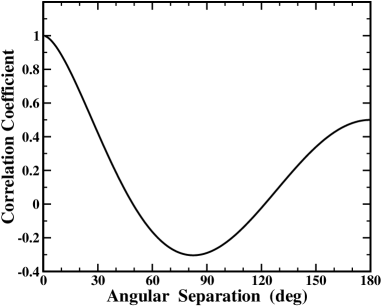
Figure 1: Expected correlation between timing residuals for a pair of pulsars as a function of separation angle[13]

Thus, a limit can be obtained in principle by a fit to correlations in the timing residuals of several pairs of pulsars with varying angular separations[33].

2.4 Models of SGWB and characteristic strain spectrum

While ground and space-based detectors are sensitive to GW generated by sources, such as supernovae, spinning neutron stars, in-spirals of extreme mass binary systems, coalescing binaries and binaries with neutron stars and black holes and super-massive black hole binaries (SMBH), the most probable sources for PTA are SMBH. Galaxy mergers during the history of universe can lead to the central SMBH in these galaxies to become gravitationally bound as a SMBH binary and generate GW during its late time in-spiral. A PTA can potentially detect GW from such SMBH with orbital periods of 10⁸ s.

A large number of SMBH are predicted by the theories of formation and evolution of SMBH. The most likely source for PTAs is the SGWB resulting from an incoherent addition of GW generated by a number of such SMBH systems[34, 29]. The characteristics strain spectrum for such a background is given by Eq. 7, with the power law index, $\alpha$ = -2/3[29].

Alternatively, PTAs are sensitive enough to detect SGWB due to other models. One such alternative is the quantum-mechanical generation of cosmological perturbations[35]. The power law index, $\alpha$, in the Eq. 7 is -1 corresponding to the parameter $\beta=$ -2 characterising the power law evolution of the cosmological scale factor, $a$, with the cosmic time (See Eq. 2 of Ref. 35). Another alternative is SGWB formed by GW emitted by a network of cosmic strings[36]. The index in this case is -7/6. Therefore, PTA results can put meaningful constraints on these models.

3 Factors affecting PTA precision

Although more than 2000 pulsars have been discovered till date, it is difficult to obtain an ideal ensemble of pulsars, which satisfy all the requirements as listed in Section 4.2, to form a high precision PTA. Apart from the pulsars being typically weak radio sources, the pulsed emission from pulsar exhibits a variety of instabilities, which makes extracting extremely tiny systematic deviations, caused by GW perturbation of metric, very challenging. These factors are discussed in this section.

3.1 Rotational instabilities

Although pulsars broadly exhibit clock-like stability, their rotation is affected by small rotational irregularities. Many young pulsars (characteristic age, $\tau_{c}<$ 10⁶ yr) show sudden increase in their rotation rates, known as glitches[37, 38, 39]. The frequency change at the glitch and its post-glitch recovery complicates timing analysis. Moreover, these events occur randomly. Hence, such pulsars are excluded from PTAs.

None of older pulsars ($\tau_{c}>$ 10⁸) have been reported to glitch and these tend to have periods larger than few 100 ms. While such pulsars were previously used to put constraints on SGWB[13], the longer observations required for these pulsars to form a stable AP and changes in AP due to a variety of effects discussed later preclude their inclusion in the sample of pulsars for the PTA. Another class of old pulsars not showing glitches are the millisecond pulsars (MSPs), which are pulsars with low surface magnetic fields (B $<$ 10¹⁰ G). The short periods help in obtaining a stable AP in short observations. Hence, MSPs are ideal candidates for a PTA sample.

Many MSPs show slow wander of rotation rate over intervals ranging from months to years. This phenomena, called timing noise, is also not predictable[40]. Timing noise is “red” in character and is similar to the expected GW signature and presents a significant constraint[41]. Recently, quasi-periodic structures in timing residuals have been reported suggesting an origin intrinsic to the neutron star[42] (See Section 3.4). Hence, a systematic characterization of a much larger sample of MSPs, than being used in the present day PTAs, is required to choose the most ideal rotators.

3.2 Signal-to-noise considerations

The TOA precision depends on the radiometer noise (and signal-to-noise ratio; S/N)[43]. Hence, it is important to include strong pulsars in a PTA. On the other hand, radio pulsars are weak radio sources (typical flux density 10 mJy; 1 mJy = 10^-29 W/m²/Hz) and this restricts the number of usable pulsars. Nearby MSPs are usually chosen for most PTAs. While the higher sky background leads to higher radiometer noise at low radio frequencies, pulsars are stronger at these frequencies due to their steep spectra. Thus, the best trade-off is achieved at frequencies $>$ 1 GHz.

3.3 Propagation effects

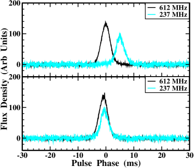
Figure 2: The TOA delay due to an error of 0.08 pc cm^-3 in assumed DM. Each panel shows the pulse obtained at 613 MHz and 237 MHz respectively with the GMRT. The upper panel shows the averaged pulse at the two frequencies with an assumed DM of 35.665 pc cm^-3, while the lower panel shows that with the estimated DM (35.740 pc cm^-3). Figure reproduced from Ref. 44

The deviation in pulsar clock are measured using the pulsed radio signal from the pulsar, which propagates through the inter-stellar medium (ISM). Radio emission is dispersed and scattered by the electrons in the ISM and encounters multi-path propagation. This smears the pulse, reduces the effective time resolution and S/N and also causes a frequency dependent delay in TOA. A combination of all these effects, due to the inhomogeneities in ISM, causes variability in pulse TOA, compromising the precision of a PTA. An illustration of these effects is shown in Fig. 2 and 3[44].

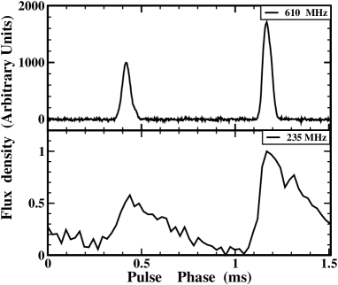
Figure 3: Scatter-broadening at low radio frequencies. Both panels show coherently dedispersed AP of MSP PSR B1937+21. The upper panel shows the AP at 610 MHz, whereas the lower panel shows the AP at 235 MHz, which is clearly scatter-broadened. Figure reproduced from Ref. 44

As pulsars are fast moving objects[45], observations of pulsars encounter different cross sections of ISM on different epochs. Fluctuation of electron density over these sections causes the dispersive delay in TOA of pulsars to vary. DM variations of the order of 0.0001 pc cm^-3 have been established in many past studies [18, 46, 47, 48, 49, 50], which correspond to variations in dispersive delay in TOA of the order of 212 ns at 1400 MHz. In addition, the line of sight to a few PTA pulsars pass close to Sun at specific epochs in a year, causing an additional dispersive delay due to the solar wind of the order of 1 $\mu$s within 7^o of the Sun[47, 48].

Appropriate corrections, estimated from observations at two or more frequencies within a few days of timing observations, for such variations are included in the timing model. The usual PTAs do not carry out such multi-frequency observations simultaneously, but the comparison of the results of such non-simultaneous observations with those from simultaneous multi-frequency observations, in progress at the GMRT, shows that the estimation uncertainties are almost identical[51].

The dispersion of the radio pulse also reduces the time resolution for the pulsar observed with the traditional filterbank instruments due to a finite channel bandwidth. Hence, PTAs utilize instruments implementing coherent dedispersion in either hardware or software, which allow even better estimation of DM variations.

Multi-path propagation of the pulsar signal leads to variable broadening of AP (Fig. 3), particularly at frequencies below 400 MHz. As this is not easily correctable, timing observations are usually carried out above 1 GHz, where this effect is negligible for low DM pulsars due to steep ($\sim\nu^{-4}$) frequency dependence of scatter-broadening.

Lastly, intensity variations, usually caused by Diffractive Inter-stellar scintillation (DISS) and Refractive Inter-stellar scintillation (RISS), affect the TOA precision. The former can be addressed by employing large bandwidths compared to scintle size, which is also desirable for higher S/N.

3.4 Intrinsic changes in pulsed emission

The pulsed emission from a pulsar is the probe of its clock mechanism provided the pulse (AP) is stable in its shape and arrival phase. Although this was broadly established in the early days of pulsar astronomy[19], observations over last four decades have shown that many pulsars switch between two or more stable APs[52]. This phenomenon is called profile mode-change. Recent studies indicate that profile mode-changes may be related to/or accompanied by changes in rotational parameters of a pulsar. Intermittent pulsars, such as PSRs B1931+24, J1841$-$0500, J1832+0029, J1839+1506, exhibit extended periods (several hundred days) with no pulsed emission and different spin-down rates for their ON and OFF epochs[53, 54, 55, 56]. A sample of 17 pulsars with profile changes corresponding to changes in spin-down rate was reported recently suggesting the cause to be switching between different magnetospheric states[42]. Lyne et al.[42] argued that the timing noise in MSPs can be explained by slow profile changes and claimed that it may be possible to correct for timing noise. In any case, the effect of the magnetospheric processes on the TOA precision poses a challenge, quite distinct from the processes related to the internal structure of neutron star, as discussed in Section 3.1, and motivates a better understanding of these processes to account for their contribution to timing residuals.

3.5 Errors in timing technique

In addition to the above effects, the timing residuals may have contributions from the clock errors in the atomic clocks used for obtaining the topocentric TOA and errors in the solar system ephemeris. See Ref. 17 for a detailed discussion on these errors. Both the ephemeris and the atomic standards are being steadily improved.

4 Requirements for a PTA experiment

The effects discussed in the last section influence the choice of pulsars and the observing instrumentation best suited for a high precision PTA. These requirements are summarised below.

4.1 Observing requirements

The appropriate instrumentation and observing strategy required for a typical PTA are

A telescope or combination of telescopes with large collecting area

Wide-band receivers, preferably with a bandwidth $>$ 1$-$2 GHz

Observing frequency between 1 to 3 GHz for the best trade-off between the influence of sky-background, steep pulsar spectra and the propagation effects

Simultaneous or near-simultaneous observations at 2 or more frequencies to calibrate DM changes, with one frequency preferably below 400 MHz

Full polarimetric observations

High time resolution receivers, employing coherent dedispersion, to eliminate the dispersion smearing of the pulse.

The frequent monitoring of a large sample of pulsars using the most sensitive telescopes requires a large amount of observing time on these, usually over-subscribed telescopes. PTAs in operations currently try to share this burden, which was also a prime motivation for forming the International Pulsar Timing Array (IPTA). Use of different observing system introduces sometimes epoch dependent variable fixed pipeline delays and clock errors. Thus, an important requirement for instrumentation is to periodically calibrate such delays.

4.2 Sample selection

The requirements for the ensemble of pulsars comprising an effective PTA are as follows

Pulsars with high signal-to-noise ratio (S/N) pulsed emission

Pulsars with stable AP

Pulsars with narrow pulses

Field MSP or MSPs in wide binaries are preferred over tight binaries to avoid relativistic effects in timing

Pulsars on line of sights without unusual ISM structures

Nearby pulsars are preferred over more distant ones

Pulsars with exceptionally high rotational stability

A reasonable distribution of pulsars mimicking the pairwise angular separation required for $\zeta(\theta_{ab})$ given by Eq. 6

The first six requirements have important implications for the precision of detection of a GW signature and are the consequences of the timing technique itself. The last two requirements are dictated by SGWB detection technique.

The short periods of MSPs combined with sharp pulses allows averaging several thousands of their pulses. MSPs also have very stable rotation and a more uniform distribution across the sky as they form a relatively local population. Hence, all PTA samples use MSPs as their ensemble.

Although more than 150 MSPs are known, the above criteria reduces the list of suitable pulsars to about 80. While this ensemble is useful, it is not ideal as most of these show systematics in timing residuals, such as timing noise. Currently, only PSR J1713+0747 shows white residuals over 5 years, with post-fit rms residuals of better than 200 ns[33, 50]. More such pulsars are required to be discovered to make an effective PTA.

5 Pulsar Timing Arrays

There are three currently active pulsar timing arrays - the Parkes Pulsar Timing Array (PPTA), the North American Nanohertz Observatory for Gravitational Waves (NANOGrav) and the European Pulsar Timing Array(EPTA). A brief description of each of these PTAs highlighting the instrumentation in use is presented in this section. The details can be found in Refs. 50, 33, 57.

5.1 The Parkes Pulsar Timing Array (PPTA)

PPTA, which started operating in 2004, was initiated by R. N. Manchester and is a collaboration between Australia Telescope National facility (ATNF), Swinburne University of Technology and several other Australian and international institutions. It uses 64-m Parkes radio telescope to time 20 MSPs every 2 to 3 weeks. The Parkes radio telescope can observe MSPs below a declination of + 25⁰ and the entire southern Galactic plane, allowing it to observe a large sample of Galactic MSPs. Observations are carried out using 20-cm, 10-cm and 50-cm receivers, the latter two frequencies coming from a dual-band coaxial receiver. All these are wide-band receivers. Wide-band backends, such as Parkes Digital Filterbank systems (PDFB1/PDFB2/PDFB3/ PDFB4) and baseband recording systems with coherent dedispersion, such as Caltech-Parkes- Swinburne-Recorder (CPSR2) and APSR are employed for the observations. See Ref. 50 and references therein for details of the observing system, instrumentation used, data reduction software and off-line processing pipeline.

5.2 The North American Nanohertz Observatory for Gravitational Waves (NANOGrav)

NANOgrav is a collaboration between National Radio Astronomy Observatories (NRAO) and several other US universities. It primarily uses 300-m Arecibo radio telescope and 100-m Green Bank Telescope(GBT) to time 35 MSPs once every twenty days at two out of 327/400/800/1400/2350 MHz wavebands. The two frequency observations are not simultaneous, but are carried out with a gap ranging from 1 hour to 7 days. Both Arecibo and GBT are very sensitive telescope, thus providing high S/N data in 15 to 45 minutes observations. Arecibo typically observes 19 pulsars and 18 pulsars are monitored by GBT. The whole ensemble is covered in 18 hours per epoch. Wide-band backends, such as Astronomical Signal Processor (ASP) or Green Bank Astronomical Signal Processor (GASP), are used to provide full polar coherently dedispersed data. See Ref. 33 and references therein for details of the observing system, instrumentation used and timing analysis.

5.3 The European Pulsar Timing Array(EPTA)

EPTA is the most recently started PTA program. It is a collaboration between several European institutions, such as Max-Planck Institute for Radio Astronomy, Jodrell Bank Centre for Astrophysics, ASTRON and so on. It uses four major European radio telescopes $-$ 70-m Lovell telescope at Jodrell Bank, 100-m Effelsberg telescope at Bonn, Westerbok Synthesis Radio Telescope and Nancy radio telescope. Sardinia Radio Telescope is likely to be added in future. There are plans to combine all these telescopes coherently to form a Large European Array for Pulsars (LEAP), which is likely to provide a telescope equivalent to 200-m single dish. See Refs. 58, 57 and references therein for details.

5.4 International Pulsar Timing Array

PTA requires frequent monitoring of pulsars at multiple radio frequencies. This adds up to a large observing time requirement from the participating radio telescopes. The pulsar community has therefore come together, in a unique initiative, to divide the required observing time across all participating telescopes and share the data. This consortium is called International Pulsar Timing Array (IPTA), which is a collaboration of the three existing PTAs - PPTA, NANOgrav and EPTA, and encompasses almost the entire pulsar community.

Apart from the division of observing time, such an international effort has other advantages and spin-offs. Firstly, this allows a fairly uniform coverage of MSPs in the north and south hemispheres. Secondly, the participating PTAs will have overlaps in their sample of MSPs, which provides consistency and quality checks on the data. Thirdly, the data from all these telescopes are brought together in public domain, which can lead to high quality data sets after proper assessment. Fourthly, this allows developing, comparing and contrasting alternative analysis techniques for data analysis through regular public data challenges. Lastly, such an effort will be very useful in developing the gravitational wave community.

IPTA monitors an ensemble of about 30 MSPs with a view to detect SGWB, mainly from super massive black hole binaries, with a detector arm length of light years in the nanohertz frequency range. Thus, it is complementary to ground (space) based detectors with typical arm length of few (millions) km and much higher frequency range.

6 Current Status of GW detection by PTAs

The currently operating PTAs are on the threshold of detection of SGWB and are already putting stringent limits to the expected strain from theoretical calculations. A large part of PTA effort has been expended in finding the “ideal” clocks for this challenging and difficult experiment. With more than 20000 TOAs on all PTA pulsars, timing residuals of the order of 30 ns have been obtained for PSRs J1713+0747 and J1909-3744[33], which show almost “white” timing residuals, demonstrating that such high timing precision is in principle achievable. These results from NANOGrav are consistent with those from PPTA[50], which also lists PSR J0437$-$4715 as a useful clock.

As discussed in Section 2.3, upper limits on characteristic strain, $h_{c}$, can be estimated from these individual measurements. These results from the PTAs are shown in Table  6. It is evident that the limits have improved substantially and are already comparable with the expected characteristic strain due to such SGWB.

Summary of limits on h_c from estimates on individual pulsars, assuming $\alpha$=$-$2/3 Source h_c(per year) Reference B1133+16 $<$ 9 $\times$ 10^-13 Ref. 13 B1237+25 B1604$-$00 B2045$-$16 B1855+09 $<$ 2 $\times$ 10^-14 Ref. 18 B1937+21 B1855+09 $<$ 1.1 $\times$ 10^-14 Ref. 30 J1713+0747 $<$ 1.1 $\times$ 10^-14 Ref. 33 J1909$-$3744 $<$ 3.9 $\times$ 10^-14 Ref. 33 B1855+09 $<$ 1.3 $\times$ 10^-14 Ref. 33 J0437$-$4715 $<$10^-15 Ref. 50 J1713+0747 $<$10^-14 Ref. 50 J1909$-$3744 $<$10^-14 Ref. 50

As discussed in Section 2.3, upper limits can also be obtained by examining the correlations in the timing residuals of several pairs of pulsars with varying angular separations. The best fit for the NANOGrav data to the Hellings & Downs correlation curve (Eq. 6) is consistent with no detectable SGWB and translates to a 2$-\sigma$ upper limit of 7.2 $\times$ 10^-15, 4.1 $\times$ 10^-15 and 3.0 $\times$ 10^-15 assuming $\alpha=-$2/3,$-$1 and $-$7/6 respectively for different models of SGWB[33]. Likewise, PPTA data are also consistent with no detectable SGWB, but with a more conservative upper limit of 6.0 $\times$ 10^-15[59].

7 Conclusions and summary

The current sensitivity of PTAs is tantalizingly close to the expected SGWB although no signature of such a background is evident from the data so far. The best “clocks” are PSR J0437$-$4715, J1713+0747 and J1909$-$3744. The most stringent limits in both methods employed in PTA are dominated by these pulsars. The real challenge for the PTA is in obtaining a larger sample of such ideal “clocks” sampling the correlation function in Fig. 1 uniformly. This motivates new surveys for finding new MSPs. New high-energy telescopes such as Fermi-LAT have already revealed a much larger population of MSPs and deeper and high time resolution radio surveys, such as HTRU survey, are underway in both the hemispheres. Another challenge is to rapidly characterise the new MSPs to be included in the future PTAs. Last, but not the least, a better understanding of magnetospheric physics of radio pulsars is required to model the variable torques on the neutron star in a bid to correct the covariant “red noise” component in the residuals contributed by such torques. While the SGWB detection still seems some years away, these efforts will certainly help advance the understanding of physics of radio pulsars as well as their environments.

References

- [1] A. Einstein, About Gravitational waves, in Proceedings of Prussian Academy of Sciences, (1918), pp. 154–167.
- [2] J. Weber, Phys. Rev. Lett. 22 (1969) 1320.
- [3] O. Jennrich et al., ESA/SRE (2011) 19.
- [4] W.-T. Ni, Int. J. Mod. Phys. D (2013) 1341004, arXiv:astro-ph/1212.2861.
- [5] K. S. Thorne, Gravitational waves, in Particle and Nuclear Astrophysics and Cosmology in the Next Millenium, eds. E. Kolb and R. Peccei. (World Scientific, Singapore, 1995), pp. 160–184.
- [6] W.-T. Ni, Mod. Phys. Lett. A 25 (2010) 922.
- [7] M. Kramer, I. H. Stairs, R. N. Manchester, M. A. McLaughlin, A. G. Lyne, R. D. Ferdman, M. Burgay, D. R. Lorimer, A. Possenti, N. D’Amico, J. M. Sarkissian, G. B. Hobbs, J. E. Reynolds, P. C. C. Freire and F. Camilo, Science 314 (2006) 97.
- [8] R. A. Hulse and J. H. Taylor, Astrophys. J. 195 (1975) L51.
- [9] J. H. Taylor and J. M. Weisberg, Astrophys. J. 253 (1982) 908.
- [10] S. Oslowski1, T. Bulik, D. Gondek-Rosinska and K. Belczynski, Mon. Not. R. Astron. Soc. 413 (2011) 461.
- [11] S. Detweiler, Astrophys. J. 234 (1979) 1100.
- [12] M. V. Sazhin, Soviet Astr. 22 (1978) 36.
- [13] R. W. Hellings and G. S. Downs, Astrophys. J. Lett. 265 (1983) L39.
- [14] R. W. Romani and J. H. Taylor, Astrophys. J. Lett. 265 (1983) L35.
- [15] R. L. Zimmerman and R. W. Hellings, Astrophys. J. 241 (1980) 475.
- [16] D. C. Backer, S. R. Kulkarni, C. Heiles, M. M. Davis and W. M. Goss, Nature 300 (1982) 615.
- [17] R. S. Foster and D. C. Backer, Astrophys. J. 361 (1990) 300.
- [18] V. M. Kaspi, J. H. Taylor and M. F. Ryba, Astrophys. J. 428 (1994) 713.
- [19] D. J. Helfand, R. N. Manchester and J. H. Taylor, Astrophys. J. 198 (1975) 661.
- [20] R. N. Manchester and J. H. Taylor, Pulsars (Freeman, San Fransisco, 1977).
- [21] A. G. Lyne and F. G. Smith, Pulsar Astronomy, 2nd edition edn. (Cambridge University Press, Cambridge, 1998).
- [22] D. Lorimer and M. Kramer, Handbook of Pulsar Astronomy (Cambridge University Press, Cambridge, 2005).
- [23] D. C. Backer and R. W. Hellings, Ann. Rev. Astron. Astrophys. 24 (1986) 537.
- [24] G. B. Hobbs, R. T. Edwards and R. N. Manchester, Mon. Not. R. Astron. Soc. 369 (2006) 655.
- [25] R. T. Edwards, G. B. Hobbs and R. N. Manchester, Mon. Not. R. Astron. Soc. 372 (2006) 1549.
- [26] F. B. Estabrook and H. D. Wahlquist, Gen. Relativ. Gravit. 6 (1975) 439.
- [27] B. Allen and J. D. Romano, Phys. Rev. D 59 (1999) 2001.
- [28] M. Maggiore, Phys. Rep. 331 (2000) 283.
- [29] A. H. Jaffe and D. C. Backer, Astrophys. J. 583 (2003) 616.
- [30] F. A. Jenet, G. B. Hobbs, W. van Straten, R. N. Manchester, M. Bailes, J. P. W. Verbiest, R. T. Edwards, A. W. Hotan, J. M. Sarkissian and S. M. Ord, Astrophys. J. 653 (2006) 1571.
- [31] F. A. Jenet, G. B. Hobbs, K. J. Lee and R. N. Manchester, Astrophys. J. Lett. 625 (2006) L123.
- [32] D. C. Backer and P. B. Demorest, Gravitational-wave astronomy with a pulsar timing array, in Frontiers of Astrophysics: A Celebration of NRAO’s 50th Anniversary, eds. A. H. Bridle, J. J. Condon and G. C. Hunt, ASP Conference Series, Vol. 395 (2008), pp. 261–270.
- [33] P. B. Demorest et al., Limits on the stochastic gravitational wave background from the north american nanohertz observatory for gravitational waves (2012), arXiv:astro-ph/1201.6641.
- [34] M. Rajagopal and R. W. Romani, Astrophys. J. 446 (1995) 543.
- [35] L. P. Grishchuk, Phys. U. 48 (2005) 1235.
- [36] T. Damour and A. Vilenkin, Phys. Rev. D 71 (2005) 063510.
- [37] S. L. Shemar and A. G. Lyne, Mon. Not. R. Astron. Soc. 282 (1996) 677.
- [38] A. Krawczyk, A. G. Lyne, J. A. Gil and B. C. Joshi, Mon. Not. R. Astron. Soc. 340 (2003) 1087.
- [39] C. M. Espinoza, A. G. Lyne, B. W. Stappers and M. Kramer, Mon. Not. R. Astron. Soc. 414 (2011) 1679.
- [40] G. Hobbs, A. G. Lyne and M. Kramer, Mon. Not. R. Astron. Soc. 402 (2010) 1027.
- [41] R. M. Shannon and J. M. Cordes, Astrophys. J. 725 (2010) 1607.
- [42] A. Lyne, G. Hobbs, M. Kramer, I. Stairs and B. Stappers, Science 329 (2010) 408.
- [43] J. H. Taylor, Phil. Trans. R. Soc. 341 (1992) 117.
- [44] B. C. Joshi and S. Ramakrishna, Bull. Astron. Soc. India 34 (2006) 401.
- [45] A. G. Lyne and D. R. Lorimer, Nature 369 (1994) 127.
- [46] A. L. Ahuja, Y. Gupta, D. Mitra and A. K. Kembhavi, Mon. Not. R. Astron. Soc. 357 (2005) 1013.
- [47] X. P. You et al., Mon. Not. R. Astron. Soc. 378 (2007) 493.
- [48] X. P. You, G. B. Hobbs, W. A. Coles, R. N. Manchester and J. L. Han, Astrophys. J. 671 (2007) 907.
- [49] M. J. Keith et al., Measurement and correction of variations in interstellar dispersion in high-precision pulsar timing (2012), arXiv:astro-ph/1211.5887.
- [50] R. N. Manchester et al., The parkes pulsar timing array project (2012), arXiv:astro-ph/1210.6130.
- [51] U. Kumar et al., private comm.
- [52] A. G. Lyne, Mon. Not. R. Astron. Soc. 153 (1971) 27.
- [53] M. Kramer, A. G. Lyne, J. T. O’Brien, C. A. Jordan and D. R. Lorimer, Science 312 (2006) 549.
- [54] F. Camilo, S. M. Ransom, S. Chatterjee, S. Johnston and P. Demorest, Astrophys. J. 746 (2012) 63.
- [55] D. R. Lorimer, A. G. Lyne, M. A. McLaughlin, M. Kramer, G. G. Pavlov and C. Chang, Astrophys. J. 758 (2012) 141L.
- [56] M. P. Surnis, B. C. Joshi, M. A. McLaughlin and V. Gajjar, Discovery of an intermittent pulsar: Psr j1839+15 (2012), arXiv:astro-ph/1210.3784.
- [57] R. van Haasteren et al., Mon. Not. R. Astron. Soc. 414 (2011) 3117.
- [58] R. D. Ferdman, Class. Quantum Grav. 27 (2010) 084014.
- [59] D. R. B. Yardley et al., Mon. Not. R. Astron. Soc. 414 (2011) 1777.