Acceleration in Weyl integrable spacetime

Abstract

We study homogeneous and isotropic cosmologies in a Weyl spacetime. It is shown that in Weyl integrable spacetime, the corresponding scalar field may act as a phantom field. In this circumstance the Weyl field gives rise to a late accelerated expansion of the Universe for all initial conditions and for a wide range of the parameters.

1 Introduction

A major effort in theoretical cosmology is a satisfactory explanation of the late-time acceleration of the universe. No convincing theory has yet been constructed to explain this state of affairs. The proposed models, characterized by a departure from conventional cosmology, either assume the existence of dark energy [1, 2], or require a modification of general relativity at cosmological distance scales [3, 4], (cf. [5]-[8] for comprehensive reviews and references). Less explored is the idea that the geometry of spacetime is not the so far assumed Lorentz geometry (see for example [9, 10, 11]). In this circumstance we need not only look for a new idea, but also revisit every type of the old models from a new viewpoint. Weyl geometry is certainly one candidate to be reviewed and reanalyzed. According to the Ehlers, Pirani and Schild proposed set of axioms [12], Weyl geometry is the natural space-time structure that follows from a small number of basic assumptions of two observable quantities: the worldlines of light rays and free falling particles [13, 14].

We recall that a Weyl space is a manifold endowed with a metric $\mathbf{g}$ and a symmetric connection $\mathbf{\nabla}$ which are interrelated via

$$\nabla_{\mu}g_{\alpha\beta}=-Q_{\mu}g_{\alpha\beta},$$

where the 1-form $Q_{\mu}$ is customarily called Weyl covariant vector field (see for example [15, 16] and the Appendix in [11] for a detailed exposition of the techniques involved in Weyl geometry). We denote by $D$ the Levi-Civita connection of the metric $g_{\alpha\beta}$. If $Q_{\mu}$ is a gradient, i.e., if $Q_{\mu}=\partial_{\mu}\phi$ for some scalar function $\phi,$ the corresponding space is called Weyl integrable spacetime. Integrable Weyl geometry does not suffer from the so-called second clock effect and for that reason it has been used in some approaches to gravitation and cosmology [17]-[27].

In this short paper we study Friedmann-Robertson-Walker (FRW) cosmologies in a Weyl framework. We demonstrate that the simple model based on the Lagrangian (1), may provide a mechanism of late accelerating expansion.

2 A simple Lagrangian

The field equations obtained from the Lagrangian $L=R$ in a Weyl spacetime constitute the generalization of the Einstein equations in vacuum (cf. eqs (30) and (31) in [28]). More general Lagrangians have also been suggested, especially in the context of the Palatini formalism, for example $L=e^{-\phi}R$ in [29]; $L=R+\beta R^{2}-2\Lambda$ gravity for FRW models was investigated in [30]; see also [31] for a formulation of a theory invariant with respect to Weyl transformations and [32] for the inclusion of torsion. There is however an alternative view, namely that the pair $\left(Q,\mathbf{g}\right)$ which defines the Weyl spacetime also enters into the gravitational theory and therefore, the field $Q$ must be contained in the Lagrangian independently from $\mathbf{g.}$ In the case of integrable Weyl geometry, i.e. when $Q_{\mu}=\partial_{\mu}\phi$ where $\phi$ is a scalar field, the pair $\left(\phi,g_{\mu\nu}\right)$ constitutes the set of fundamental geometrical variables. We stress that the nature of the scalar field is purely geometric.

A simple Lagrangian involving the set $\left(\phi,g_{\mu\nu}\right)$ is given by

$$L=R+\xi\nabla_{\mu}Q^{\mu}+L_{m},$$ (1)

where $\xi$ is a constant and $L_{m}$ corresponds to the Lagrangian yielding the energy-momentum tensor of a perfect fluid. Motivations for considering theory (1) can be found in [33, 34] (see also [35, 36, 37] for a multidimensional approach and [38] for an extension of (1) to include an exponential potential function of $\phi$). The inclusion of the term $\xi\nabla_{\mu}Q^{\mu}$ in the Lagrangian is not an arbitrary choice, as is explained in [39]. In fact, apart from the scalar curvature $R,$ there are two invariants with dimension of inverse squared length that can be constructed with the fundamental geometrical variables of a Weyl space: $\nabla_{\mu}Q^{\mu}$ and $Q_{\mu}Q^{\mu}.$ Now the derivative operator $\nabla_{\mu}$ can be expressed in terms of the Levi-Civita derivative operator $D_{\mu},$ so that, $\nabla_{\mu}Q^{\mu}=D_{\mu}Q^{\mu}+2Q_{\mu}Q^{\mu},$ (see the list of identities in the Appendix in [11]). Therefore the two invariants reduce to one. We conclude that the simplest vacuum Lagrangian constructed from purely geometric quantities has the form $L=R+\xi\nabla_{\mu}Q^{\mu}$.

By varying the action corresponding to (1) with respect to both $g_{\mu\nu}$ and $\phi$ one obtains [34, 38]

$$\overset{\circ}{G}_{\mu\nu}=\frac{3-4\xi}{2}\left(\partial_{\mu}\phi\partial_{\nu}\phi-\frac{1}{2}\left(\partial_{\alpha}\phi\partial^{\alpha}\phi\right)g_{\mu\nu}\right)+T_{\mu\nu},$$ (2)

and

$$\overset{\circ}{\square}\phi=\frac{1}{4\xi-3}\rho,$$ (3)

where the accent $\overset{\circ}{}$ denotes a quantity formed with the Levi-Civita connection, $D$. As mentioned above, ordinary matter described by $T_{\mu\nu}$ is a perfect fluid with energy density $\rho$ and pressure $p$. Setting

$$\lambda=\frac{4\xi-3}{2},$$

we note that for $\lambda<0$ the field equations are formally equivalent to general relativity with a massless scalar field coupled to a perfect fluid. On the other hand the case $\lambda>0$, is more interesting, because the Weyl field $\phi$ plays the role of a phantom scalar field characterized by the “wrong” sign of the kinetic term. We emphasize that the scalar field has a geometric nature in Weyl spacetime and therefore, no restriction exists for the sign of the value of $\lambda$. In the following we consider only the case of positive $\lambda$.

3 Acceleration of FRW models

We assume an initially expanding FRW universe with expansion scale factor $a\left(t\right)$ and Hubble function $H=\dot{a}/a$. We adopt the metric and curvature conventions of [41]. An overdot denotes differentiation with respect to time $t,$ and units have been chosen so that $c=1=8\pi G.$ Ordinary matter is described by a perfect fluid supplemented with an equation of state,

$$p=(\gamma-1)\rho,\ \ \ 0<\gamma<2.$$

The field equations (2) and (3) imply the Friedmann equation,

$$H^{2}+\frac{k}{a^{2}}=\frac{1}{3}\rho-\frac{\lambda}{6}\dot{\phi}^{2},$$ (4)

with $k=-1,0,+1,$ the Raychaudhuri equation,

$$\dot{H}=-\frac{\gamma}{2}\rho+\frac{\lambda}{2}\dot{\phi}^{2}+\frac{k}{a^{2}},$$

the equation of motion of the scalar field,

$$\ddot{\phi}+3H\dot{\phi}=-\frac{1}{2\lambda}\rho,$$

and the conservation equation,

$$\dot{\rho}=-3\gamma\rho H-\frac{1}{2}\rho\dot{\phi}.$$

We introduce expansion-normalized variables

$$x=\frac{\dot{\phi}}{\sqrt{6}H},\ \ \ \ \Omega=\frac{\rho}{3H^{2}},\ \ \ \ K=\frac{k}{H^{2}a^{2}},$$ (5)

and a new time variable $\tau$ defined by $\tau=\ln a.$ For flat, $k=0,$ models the dynamical system becomes

$$x^{\prime} =-3x-\sqrt{\frac{3}{2}}\frac{1}{2\lambda}\Omega+x\left(\frac{3\gamma}{2}\Omega-3\lambda x^{2}\right),$$

$$\Omega^{\prime} =\Omega\left(-3\gamma-\sqrt{\frac{3}{2}}x+3\gamma\Omega-6\lambda x^{2}\right),$$ (6)

where a prime denotes differentiation with respect to $\tau$. The evolution of the Hubble function is described by the equation,

$$H^{\prime}=-H\left(\frac{3\gamma}{2}\Omega-3\lambda x^{2}\right),$$

which decouples from the rest of the evolution equations (6). This is one of the merits of the introduction of the variables (5), namely that it allows for the reduction of the dimension of the dynamical system by one.

The constraint (4) takes the form

$$\Omega=1+\lambda x^{2}.$$ (7)

The last equation implies that the phase space of the dynamical system consists of a parabola in the $x-\Omega$ plane, i.e., it is one-dimensional. In fact, substituting (7) into the first of (6), we obtain the one-dimensional dynamical system

$$x^{\prime}=-\sqrt{\frac{3}{2}}\frac{1}{2\lambda}+3\left(\frac{\gamma}{2}-1\right)x-\frac{1}{2}\sqrt{\frac{3}{2}}x^{2}+3\left(\frac{\gamma}{2}-1\right)\lambda x^{3}.$$ (8)

The only real equilibrium of (8) is

$$x_{\ast}=-\frac{1}{\sqrt{6}\left(2-\gamma\right)\lambda}.$$ (9)

This solution was also found by Oliveira et al [38], in the context of inflation. It corresponds to a “scaling” solution where the energy density of the Weyl field is a constant fraction of the total energy density. A plot of the polynomial right-hand side of (8) shows that the equilibrium solution (9) is globally asymptotically stable, i.e., $x_{\ast}$ is the future attractor of all solutions of (8).

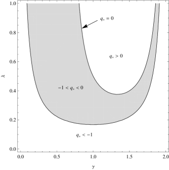
Figure 1: In region below the parabolic curve $q_{\ast}=0$, all models asymptotically expand with acceleration. The dark region corresponds to models entering a phase of late accelerating expansion and avoid the big rip singularity.

The decceleration parameter $q=-\ddot{a}a/\dot{a}^{2}$ at the equilibrium is given by

$$q_{\ast}=\frac{1+2\lambda\left(\gamma-2\right)\left(3\gamma-2\right)}{4\lambda\left(\gamma-2\right)}.$$ (10)

In Figure 1 the curve corresponding to $q_{\ast}=0,$ separates the parameter space into two disjoint regions. The region below the parabolic curve, $q_{\ast}=0$, contains the values of the parameters corresponding to accelerating expansion ($\ddot{a}>0$). It is evident that the simple model (1) allows for a late accelerated expansion of the universe for a wide range of the parameters.

4 Final remarks

In models with minimally coupled phantom fields, the density of the dark energy increases with increasing scale factor and, both the scale factor and the phantom energy density can become infinite at a finite $t$, a condition known as the “big rip”, [42, 43, 44]. Since the scale factor corresponding to the asymptotic solution (9) evolves as $t^{1/\left(1+q_{\ast}\right)},$ flat FRW models in (1) theory may avoid the big rip singularity provided that $-1<q_{\ast}$. We conclude that for any couple $\left(\gamma,\lambda\right)$ in (10) satisfying $-1<q_{\ast}<0,$ all initially expanding universes eventually enter a phase of accelerating expansion and avoid the big rip singularity. Inclusion of curvature, $k=\pm 1,$ increases the dimension of the dynamical system by one. However, it can be shown that the resulting models share the main feature of the flat model, namely that the state of the system asymptotically approaches a stable equilibrium corresponding to accelerating expansion. The results of this study are purely qualitative and therefore, further investigation is necessary to answer the question if the (1) theory may model the whole history of the Universe.

References

- [1] S. Sahni and A. Starobinsky, Int. J. Mod. Phys. D 9 (2000) 373.
- [2] P.J. Peebles, B. Ratra, Rev. Mod. Phys. 75 (2003) 559.
- [3] T. Chiba, Phys. Lett. B 575 (2003) 1.
- [4] S.M. Carroll, V. Duvvuri, M. Trodden and M.S. Turner, Phys. Rev. D 70 (2004) 043528.
- [5] E.J. Copeland, M. Sami and S. Tsujikawa, Int. J. Mod. Phys. D 15 (2006) 1753.
- [6] T. Sotiriou and V. Faraoni, Rev. Mod. Phys. 82 (2010) 451.
- [7] A. De Felice and S. Tsujikawa, Living Rev. Rel. 13 (2010) 3.
- [8] K. Bamba, S. Capozziello, S. Nojiri and S.D. Odintsov, Astrophys. Space Sci. 342 (2012) 155.
- [9] S. Capozziello, S. Carloni and A. Troisi, Preprint astro-ph/0303041.
- [10] S. Capozziello, R. Cianci, C. Stornaiolo and S. Vignolo, Phys. Scripta 78 (2008) 065010.
- [11] J. Miritzis, Class. Quantum Grav. 21 (2004) 3043.
- [12] J. Ehlers, F.A.E. Pirani and A. Schild, in General Relativity, Papers in honour of J.L. Synge, pp. 63-82, Clarendon Press, Oxford U.K. 1972.
- [13] M. Di Mauro, L. Fatibene, M. Ferraris and M. Francaviglia, Int. J. Geom. Meth. Mod. Phys. 7 (2010) 887.
- [14] L. Fatibene and M. Francaviglia, arXiv:1106.1961.
- [15] J.A. Schouten, Ricci Calculus, Springer-Verlag, Berlin, 1954.
- [16] P. Gilkey, S. Nikčević and U. Simon, J. Geom. Phys. 61 (2011) 270.
- [17] M. Novello and H. Heintzmann, Phys. Lett. A 98 (1983) 10.
- [18] V. Perlick, Class. Quantum Grav. 8 (1991) 1369.
- [19] V. Hamity and D. Barraco, Gen. Rel. Grav. 25 (1993) 461.
- [20] J.M. Salim and S.L. Sautu, Class. Quantum Grav. 15 (1998) 203.
- [21] J.M. Salim and S.L. Sautu, Class. Quantum Grav. 16 (1999) 3281.
- [22] O. Arias, R. Cardenas and I. Quiros, Nucl. Phys. B 643 (2002) 187.
- [23] M. Israelit, Found. Phys. 35 (2005) 1725.
- [24] F. Dahia, G.A.T. Gomez and C. Romero, J. Math. Phys. 49 (2008) 102501.
- [25] T.Y. Moon, J. Lee and P. Oh, Mod. Phys. Lett. A 25 (2010) 3129.
- [26] C. Romero, J.B. Fonseca-Neto and M.L. Pucheu, Found. Phys. 42 (2012) 224.
- [27] I. Quiros, R. Garcia-Salcedo, J.E.M. Aguilar and T. Matos, Gen. Rel. Grav. (2012) arXiv:1108.5857.
- [28] S. Cotsakis, J. Miritzis and L. Querella, J. Math. Phys. 40 (1999) 3063.
- [29] F.P. Poulis and J.M. Salim, Int. J. Mod. Phys. Conf. Series V.3 (2011) 87.
- [30] R. Gannouji, H. Nandan and N. Dadhich, J. Cosmol. Astropart. Phys. 11 (2011) 051.
- [31] C. Romero, J.B. Fonseca-Neto and M.L. Pucheu, Class. Quantum Grav. 29 (2012) 155015.
- [32] J. B. Fonseca-Neto, C. Romero and S.P.G. Martinez, arXiv:1211.1557.
- [33] M. Novello, L.A.R. Oliveira, J.M. Salim and E. Elbas, Int. J. Mod. Phys. D 1 (1993) 641.
- [34] J.M. Salim and S.L. Sautu, Class. Quantum Grav. 13 (1996) 353.
- [35] M.Y. Konstantinov and V.M. Melnikov, Int. J. Mod. Phys. D 4 (1995) 339.
- [36] J.E.M. Aguilar and C. Romero, Found. Phys. 39 (2009)1205.
- [37] J.E.M. Aguilar and C. Romero, Int. J. Mod. Phys. A 24 (2009)1505.
- [38] H.P. Oliveira, J.M. Salim and S.L. Sautu, Class. Quantum Grav. 14 (1997) 2833.
- [39] M. Novello and S.E.P. Bergliaffa, Phys. Rept. 463 (2008) 127.
- [40] J. Miritzis arXiv: 1301.5402
- [41] J. Wainwright and G.F.R. Ellis, Dynamical Systems in Cosmology, Cambridge University Press, 1997.
- [42] S. Nojiri, S.D. Odintsov and S. Tsujikawa, Phys. Rev. D 71 (2005) 063004.
- [43] M.R. Setare and E.C. Vagenas, Astrophys. Space Sci. 330 (2010) 145.
- [44] P.H. Frampton, K.J. Ludwick, S. Nojiri, S.D. Odintsov and R.J. Scherrer, Phys. Lett. B 708 (2012) 204.