Analytical results from the quantum theory of a single-emitter nanolaser. II.

Abstract

Using two equivalent approaches, Heisenberg-Langevin and density operator, we investigate the properties of nanolaser: an incoherently pumped single two-level system interacting with a single-cavity mode of finite finesse. We show that in the case of good-cavity regime the Heisenberg-Langevin approach provides the analytical results for linewidth, amplitude fluctuation spectrum, and intracavity Mandel Q-parameter. In the bad-cavity regime we estimate the frequency at which the peak of relaxation oscillations appears. With the help of the master equation for density operator written in terms of coherent states we obtain approximated expression for Glauber-Sudarshan P function. This solution can be used in the case of good-cavity regime and allows us to investigate in more detail the thresholdless behaviour of the nanolaser. All two approaches are in a very good agreement with each other and numerical simulations.

I 1. INTRODUCTION

One of the first theoretical work devoted to possibility of realization of a single-emitter laser was published by Mu and Savage in Mu1992 . Three- and four-level pumped emitters placed into lossy cavity and interacted with cavity mode have been considered there. Some interesting effects which do not appear in conventional lasers have been revealed, such as squeezing, self-quenching in incoherently pumped laser, deviations from the Schawlow-Townes formula for the linewidth. Subsequent publications related to single-emitter problem Ginzel1993 ; Pellizari1994 ; Loffler1997 ; Jones1999 ; Clemens2004 ; Kilin2001 ; Kilin2002 ; Kilin2012 have proven these results and also discovered new effects connected with the presence of one emitter: vacuum-Rabi doublet in the spectrum Ginzel1993 ; Loffler1997 , lasing without inversion Kilin2001 , entanglement between emitter and field subsystems Kilin2002 . In most of these works results have been obtained with help of different type of numerical methods applied to the master equation for density operator or to the Heisenberg-Langevin equations.

Nowadays a single-emitter laser is realized in experiments where the role of emitter can play the single atom McKeever2003 , or ion Dubin2010 or quantum dot Nomura2009 . In this connection, the purpose of our paper is to provide analytical results which can be considered as a tools for experimenter. Thus in our previous Brief Report Larionov2011 with help of the Heisenberg-Langevin approach we obtained analytical expressions for linewidth, amplitude fluctuation spectrum and Mandel Q parameter, which describe the behaviour of a single-emitter laser in the case of good cavity regime. We also improved the condition required for thresholdless regime. In this paper in Sec. 2 we will consider and analyze in more detail the linearization procedure which we used earlier and extend our calculations to bad-cavity regime. In Sec. 3 we will write master equation for our nanolaser in the coherent state representation and in stationary regime derive approximated expression for Glauber-Sudarshan P function. With the help of the latter we will prove our previous results, analyze some limited cases and threshold behaviour of nanolaser.

II 2. HEISENBERG-LANGEVIN APPROACH

II.1 2.1 Model. Semiclassical theory

The simplest model of a single-emitter nanolaser is the single two-level system placed inside the single-mode cavity and incoherently pumped to its upper level. Just four constants characterize this nanolaser: $\Gamma$ – the incoherent pumping rate, pumping process associated with the transition $\left|1\right\rangle\rightarrow\left|2\right\rangle$; $\gamma/2$ – the decay rate of polarization due to spontaneous emission to modes other than the laser mode; $\kappa/2$ – the field decay rate in the cavity; $g$ – the coupling constant between the field and the two-level system. The Heisenberg-Langevin equations for our nanolaser are

$$\frac{d}{dt}\hat{a}(t) = -\frac{\kappa}{2}\hat{a}(t)+g\hat{\sigma}(t)+\hat{f}_{a}(t),$$

$$\frac{d}{dt}\hat{\sigma}(t) = -\frac{1}{2}(\Gamma+\gamma)\hat{\sigma}(t)+g\hat{D}(t)\hat{a}(t)+\hat{f}_{\sigma}(t),$$

$$\frac{d}{dt}\hat{D}(t) = \Gamma-\gamma-(\Gamma+\gamma)\hat{D}(t)$$ (1)

$$- 2g\Bigl{[}\hat{\sigma}^{{\dagger}}(t)\hat{a}(t)+\hat{a}^{{\dagger}}(t)\hat{\sigma}(t)\Bigr{]}+\hat{f}_{D}(t).$$

Here $\hat{a}(t)$ and $\hat{a}^{{\dagger}}(t)$ are the photon annihilation and creation operators in the cavity mode, $\hat{\sigma}=|1\rangle\langle 2|$ is the operator of polarization of the two-level system, and $\hat{D}=|2\rangle\langle 2|-|1\rangle\langle 1|$ is the operator of inversion between the upper level $|2\rangle$ and the lower level $|1\rangle$ of the system. We use the fact that for a single two-level system $|2\rangle\langle 2|+|1\rangle\langle 1|=\mathbf{I}$ - where $\mathbf{I}$ is a unity operator.

The $\hat{f}_{a}\left(t\right)$, $\hat{f}_{\sigma}\left(t\right)$ and $\hat{f}_{D}\left(t\right)$ are the Langevin noise operators which arise through the interaction with the heat baths. Using the standard quantum-optical methods (see, for example, Refs. methods ), we obtain the following nonzero correlation functions of these operators:

$$\langle\hat{f}_{a}(t)\hat{f}^{{\dagger}}_{a}(t^{\prime})\rangle = \kappa\delta(t-t^{\prime}),$$

$$\langle\hat{f}^{{\dagger}}_{\sigma}(t)\hat{f}_{\sigma}(t^{\prime})\rangle = \Gamma\delta(t-t^{\prime}),$$

$$\langle\hat{f}_{\sigma}(t)\hat{f}^{{\dagger}}_{\sigma}(t^{\prime})\rangle = \gamma\delta(t-t^{\prime}),$$ (2)

$$\langle\hat{f}_{\sigma}(t)\hat{f}_{D}(t^{\prime})\rangle = 2\gamma\langle\hat{\sigma}(t)\rangle\delta(t-t^{\prime}),$$

$$\langle\hat{f}_{D}(t)\hat{f}_{\sigma}(t^{\prime})\rangle = -2\Gamma\langle\hat{\sigma}(t)\rangle\delta(t-t^{\prime}),$$

$$\langle\hat{f}^{{\dagger}}_{\sigma}(t)\hat{f}_{D}(t^{\prime})\rangle = -2\Gamma\langle\hat{\sigma}^{{\dagger}}(t)\rangle\delta(t-t^{\prime}),$$

$$\langle\hat{f}_{D}(t)\hat{f}^{{\dagger}}_{\sigma}(t^{\prime})\rangle = 2\gamma\langle\hat{\sigma}^{{\dagger}}(t)\rangle\delta(t-t^{\prime}),$$

$$\langle\hat{f}_{D}(t)\hat{f}_{D}(t^{\prime})\rangle = 2[(\Gamma+\gamma)-(\Gamma-\gamma)\langle\hat{D}(t)\rangle]\delta(t-t^{\prime}).$$

We are also interested in the field properties transmitted outside the cavity through the outcoupling mirror. For that we should consider the annihilation operator $\hat{a}_{\rm{out}}(t)$ of photons outside the cavity Gardiner2000 . The input-output transformation is

$$\hat{a}_{\rm out}(t)=\sqrt{\kappa}\hat{a}(t)-\hat{f}_{a}(t)/\sqrt{\kappa}.$$ (3)

In the next Sec. 2.2 we will applied linearization procedure to Eq. (1) which allows us to investigate the small fluctuations of laser field near the dominant stationary semiclassical mean value. To find the latter for our nanolaser we need to collect a large number of photons in the cavity and also provide the coherent interaction of each photon with the single emitter.

In the assumption that above two conditions are satisfied let us obtain the stationary semiclassical solution from Eq. (1). For that we need to drop all time derivatives $d\hat{X}/dt$ and average the remained stationary equations under assumption of following decorrelations $\left\langle\hat{D}\hat{a}\right\rangle=\left\langle\hat{D}\right\rangle\left\langle\hat{a}\right\rangle$, $\left\langle\hat{\sigma}^{{\dagger}}\hat{a}\right\rangle=\left\langle\hat{\sigma}^{{\dagger}}\right\rangle\left\langle\hat{a}\right\rangle$. Suppose that in steady state the optical phase is randomly distributed between $0$ and $2\pi$ we take the average value of operators with the fixed arbitrary mean value of the phase to be equal to zero $\varphi_{0}=0$. Such selection of the phase value implies the reality of semiclassical field amplitude $a_{0}$ and polarization $\sigma_{0}=\frac{\kappa}{2g}a_{0}$. Thus, the analytical expression for semiclassical stationary intracavity intensity $I_{0}=|a_{0}|^{2}$ is therefore

$$I_{0}=\frac{I_{s}}{2}\left[(r-1)-\frac{(r+1)^{2}}{c}\right].$$ (4)

where we introduce new dimensionless parameters: the dimensionless pumping rate $r=\Gamma/\gamma$; the dimensionless saturation intensity $I_{s}=\gamma/\kappa$; the dimensionless coupling strength $c=4g^{2}/\kappa\gamma$.

Eq. (4) coincides with one firstly obtained by Mu and Savage Mu1992 . $I_{0}\left(r\right)$ is a parabolic function of pump rate which has physical interpretation when $c>8$ and when the value of the pump rate lying in the domain between two points, so called threshold $r_{th}$ and self-quenching $r_{q}$ points, which are given by the following expressions

$$r_{th}=r_{m}-\frac{c}{2}\sqrt{1-8/c},\text{ }r_{q}=r_{m}+\frac{c}{2}\sqrt{1-8/c},$$ (5)

where $r_{m}=c/2-1$ is the point where the stationary solution has a maximum $I_{m}=I_{s}\left(c/8-1\right)$.

The stationary intensity $I_{0}\left(r\right)$ increases as a pump is increased and it starts from the threshold point $r_{th}$. When $c\gg 8$ then $r_{th}\approx 1+4/c$, what indicates on finite value of the threshold or, in other words, there is no thresholdless regime in this semiclassical model. The self-quenching point $r_{q}$ corresponds to pumping rate where the atomic polarization is rapidly damped to zero due to emitter trapping in the excited state, what leads to the damping of the field.

From the expression for the maximum of intensity $I_{m}$ it follows that large mean number of photons in the cavity can be achieved when $cI_{s}\gg 8$ (we assumed that $c\gg 8$). The latter condition can be written in other form $g\gg\kappa$. Thus the semiclassical regime takes place when the photons lifetime in the cavity is so long that each photon is provided by coherent interaction with the single emitter (above mentioned condition). The condition $cI_{s}\gg 8$ also gives us possibility to collect a large mean number of photons in two opposite cases, namely in good - $I_{s}\gg 1$ and bad-cavity regimes $I_{s}\ll 1$.

II.2 2.2 Linearization around the stationary solution

To linearize the Heisenberg-Langevin equations (1) we assume that all operators can be presented as a sum of dominant classical term $X_{0}$ and a "small" operator valued fluctuation $\delta\hat{X}$ (see, for example, Refs. Kolobov1993 ; Haake1996 ),

$$\hat{X}=X_{0}+\delta\hat{X}.$$ (6)

After linearization with respect to $\delta\hat{X}$ we obtain the following equations for the fluctuations

$$\frac{d}{dt}\delta\hat{a}(t)= - \frac{\kappa}{2}\delta\hat{a}(t)+g\delta\hat{\sigma}(t)+\hat{f}_{a}(t),$$

$$\frac{d}{dt}\delta\hat{\sigma}(t)= - \frac{1}{2}(\Gamma+\gamma)\delta\hat{\sigma}(t)+g\Bigl{[}a_{0}\delta\hat{D}(t)+D_{0}\delta\hat{a}(t)\Bigr{]}$$

$$+ \hat{f}_{\sigma}(t),$$

$$\frac{d}{dt}\delta\hat{D}(t)= - (\Gamma+\gamma)\delta\hat{D}(t)-2g\Bigl{[}\sigma_{0}(\delta\hat{a}(t)+\delta\hat{a}^{{\dagger}}(t))$$ (7)

$$+ a_{0}(\delta\hat{\sigma}(t)+\delta\hat{\sigma}^{{\dagger}}(t)\Bigr{]}+\hat{f}_{D}(t).$$

Before solving Eqs. (7) we first split operators into Hermitian "real" and "imaginary" parts as

$$\delta\hat{a}(t) = \delta\hat{u}(t)+i\delta\hat{\nu}(t),$$

$$\delta\hat{\sigma}(t) = \delta\hat{\mu}(t)+i\delta\hat{\eta}(t),$$

$$\hat{f}(t) = \hat{\Sigma}(t)+i\hat{\Delta}(t).$$ (8)

In this way the linearized equations of motion separate into two independent blocks

$$\frac{d}{dt}\delta\hat{u}(t)= - \frac{\kappa}{2}\delta\hat{u}(t)+g\delta\hat{\mu}(t)+\hat{\Sigma}_{a}(t),$$

$$\frac{d}{dt}\delta\hat{\mu}(t)= - \frac{1}{2}(\Gamma+\gamma)\delta\hat{\mu}(t)+g\Bigl{[}a_{0}\delta\hat{D}(t)+D_{0}\delta\hat{u}(t)\Bigr{]}$$

$$+ \hat{\Sigma}_{\sigma}(t),$$

$$\frac{d}{dt}\delta\hat{D}(t)= - (\Gamma+\gamma)\delta\hat{D}(t)-4g\Bigl{[}\sigma_{0}\delta\hat{u}(t)+a_{0}\delta\hat{\mu}(t)\Bigr{]}$$ (9)

$$+ \hat{f}_{D}(t);$$

$$\frac{d}{dt}\delta\hat{\nu}(t) = -\frac{\kappa}{2}\delta\hat{\nu}(t)+g\delta\hat{\eta}(t)+\hat{\Delta}_{a}(t),$$

$$\frac{d}{dt}\delta\hat{\eta}(t) = -\frac{1}{2}(\Gamma+\gamma)\delta\hat{\eta}(t)+gD_{0}\delta\hat{\nu}(t)+\hat{\Delta}_{\sigma}(t).$$

We want to note that the independence of "real" and "imaginary" parts is a result of our phase selection in the derivation of semiclassical solution (see Eq. (4) and text above).

The block for three real parts $\delta\hat{u}$, $\delta\hat{\mu}$, $\delta\hat{D}$ are related to the intensity fluctuations via $\delta\hat{I}=2a_{0}\delta\hat{u}$. The two imaginary parts $\delta\hat{\nu}$, $\delta\hat{\eta}$ can be associated with phase fluctuations.

Eqs. (9, LABEL:Im_Block) can be resolved by means of Fourier transformation. For that we need to perform the fluctuations as

$$\delta\hat{X}(t)=\int_{-\infty}^{\infty}\delta\hat{X}(\Omega)\exp(-i\Omega t)\frac{d\Omega}{2\pi},$$ (11)

which gives us the linear algebraic equations which can be resolved by means of Cramer’s rule. The result for the Fourier-transformed amplitude $\delta\hat{u}$ and phase $\delta\hat{\nu}$ quadrature components are

$$\delta\hat{u}(\Omega) = \frac{\hat{\Sigma}_{a}(\Omega)A(\Omega)+\hat{\Sigma}_{\sigma}(\Omega)C(\Omega)+\hat{f}_{D}(\Omega)B}{i\Omega\Bigl{[}(i\Omega-(\Gamma+\gamma+\kappa))/2)(i\Omega-(\Gamma+\gamma))+4g^{2}|a_{0}|^{2}\Bigr{]}-4\kappa g^{2}|a_{0}|^{2}},$$ (12)

$$\delta\hat{\nu}(\Omega) = \frac{g\hat{\Delta}_{\sigma}(\Omega)-\hat{\Delta}_{a}(\Omega)(i\Omega-(\Gamma+\gamma)/2)}{i\Omega\Bigl{[}i\Omega-(\Gamma+\gamma+\kappa)/2\Bigr{]}},$$ (13)

where

$$A(\Omega) = -[(i\Omega-(\Gamma+\gamma)/2)(i\Omega-(\Gamma+\gamma))+4g^{2}|a_{0}|^{2}],$$

$$C(\Omega) = g(i\Omega-(\Gamma+\gamma)),\text{ }B=-g^{2}a_{0}.$$ (14)

As it follows from the correlation function definition Eqs. (2) and from Eq. (11) the Fourier-transformed quadrature components $\delta\hat{u}$, $\delta\hat{\nu}$ are $\delta$-function correlated. Using the input-output transformation Eq. (3) we find the amplitude and phase fluctuation spectra

$$\langle\delta\hat{u}_{\rm{out}}(\Omega)\delta\hat{u}_{\rm{out}}(\Omega^{\prime})\rangle=\frac{1}{4}\delta(\Omega+\Omega^{\prime})\Bigl{[}1+\frac{\kappa^{2}}{4}\frac{a\Omega^{2}+b\gamma^{2}}{\Omega^{2}(\Omega^{2}-d)^{2}+\gamma^{2}(e\Omega^{2}-f)^{2}}\Bigr{]},$$ (15)

$$\langle\delta\hat{\nu}_{\rm{out}}(\Omega)\delta\hat{\nu}_{\rm{out}}(\Omega^{\prime})\rangle=\frac{1}{4}\delta(\Omega+\Omega^{\prime})\Bigl{[}1+\frac{\kappa^{2}}{4}\frac{\gamma^{2}[c(r+1)+(r+1)^{2}]}{\Omega^{2}(\Omega^{2}+\gamma^{2}(r+1+1/I_{s})^{2}/4)}\Bigr{]},$$ (16)

where

$$a = \gamma^{2}[c(r-1)-(r+1)^{2}+2cr],$$

$$b = \gamma^{2}(r-1)[3(r+1)^{3}+2c^{2}-c(r+1)(r-5)],$$

$$d = \gamma^{2}\frac{cI_{s}(r-1)+(r+1)}{2I_{s}},\text{ }e=\frac{3(r+1)+1/I_{s}}{2},$$

$$f = \gamma^{2}cI_{0}/I_{s}^{2}.$$ (17)

Now we will use these results to analyze two different regimes of our nanolaser, namely good- and bad-cavity regimes.

II.3 2.3 Good-cavity regime

In the case of good-cavity regime $I_{s}\gg 1$ the obtained expression for the amplitude fluctuation spectrum Eq. (15) becomes

$$\langle\delta\hat{u}_{\rm{out}}(\Omega)\delta\hat{u}_{\rm{out}}(\Omega^{\prime})\rangle=\frac{1}{4}\delta(\Omega+\Omega^{\prime})\Bigl{[}1+\frac{S(r,c)}{1+(\Omega/\Omega_{0})^{2}}\Bigr{]}.$$ (18)

The first term in the square brackets corresponds to standard quantum limit (SQL), the second term is a Lorentzian with width $\Omega_{0}$ given by

$$\Omega_{0}=\kappa\Bigl{[}1-\frac{(r+1)^{2}}{c(r-1)}\Bigr{]}$$ (19)

and this term describes the additionally exes above the SQL or reduction of the noise below SQL depending of the sign of the strength $S(r,c)$

$$S(r,c)=\frac{(r-1)\left[3(r+1)^{3}+2c^{2}-c(r+1)(r-5)\right]}{\left[c(r-1)-(r+1)^{2}\right]^{2}}.$$ (20)

We have investigated this expression in order to find out a possibility of the noise reduction below the SQL in the laser light outside the cavity. Unfortunately, this kind of nonclassical phenomenon are very limited. We have found that in the region of pump parameter $r_{m}<r<r_{q}$ the strength $S(r,c)$ is always positive and increasing function, resulting in the excess noise in Eq. (18). The small negative values of $S(r,c)$ are observed when the pump parameter is centered around $r=c/5$ ($c\geq 200$), i.e. lies in the region $r_{th}\ll r<r_{m}$. Probably, these negative values are the result of the well-known antibunching phenomenon for a single-emitter. However, this antibunching effect is strongly attenuated due to the effect of accumulation of many photons inside the cavity during the long (and random) photon lifetime.

The Mandel Q-parameter can be expressed through the amplitude quadrature component $\delta\hat{u}$ as $Q=4\cdot\int_{-\infty}^{\infty}\langle\delta\hat{u}(\Omega)\delta\hat{u}(-\Omega)\rangle d\Omega/2\pi-1$ and the result is

$$Q(r,c)=\frac{1}{2}S(r,c)\left[1-\frac{(r+1)^{2}}{c(r-1)}\right].$$ (21)

We see that the strength $S(r,c)$ is also characterized this quantity. On the Fig. 1a there are some graphics for Mandel Q-parameter for different coupling constant $c$ when $I_{s}\gg 1$. For the pump rate lying between threshold and quenching points our theoretical results are in a very good agreement with the exact solution of the master equation for the density matrix (see next Sec. 3). The main divergency appears near the threshold and quenching points where the linear theory does not work. Two fluctuations peaks of Mandel Q-parameter are well known Jones1999 : first of them associated with laser turn on and second broad peak associated with laser turn off.

Another quantity of interest is the low-frequency asymptotic version of the fluctuation spectrum of the phase quadrature component. Using the Eq. (16) we obtain

$$\langle\delta\hat{\nu}_{\rm{out}}(\Omega)\delta\hat{\nu}_{\rm{out}}(\Omega^{\prime})\rangle=\delta(\Omega+\Omega^{\prime})\frac{\kappa^{2}}{4}\frac{1+c/(r+1)}{\Omega^{2}}.$$ (22)

The low-frequency divergence in this spectrum as $1/\Omega^{2}$ is manifesting for the phase diffusion process Courtois1991 . This spectrum also defines the linewidth $\Delta\nu$ of our nanolaser through $\langle(\delta\hat{\nu}_{\rm{out}})^{2}\rangle_{\Omega}/I_{0}$

$$\Delta\nu=\Delta\nu_{\rm{ST}}\frac{1}{2}\left(1+\frac{c}{r+1}\right),$$ (23)

where $\Delta\nu_{\rm{ST}}=\kappa/(2I_{0})$ is the Schawlow-Townes linewidth of a conventional incoherently pumped laser. The obtained formula for the linewidth shows the deviation from the Schawlow-Townes result and this coincides with the numerical simulations performed by Clemens et al Clemens2004 .

At the end of this section we want to discuss the legality of above linearization procedure. Let us explain it in terms of adiabatic elimination of the emitter variables in Eq. (1). Indeed, in the case when $I_{s}\gg 1$ one can obtain the Heisenberg-Langevin equation only for the field operator $\hat{a}(t)$. The semiclassical solution of the latter coincides with Eq. (4). The following linearization with respect to fluctuation $\delta\hat{a}(t)$ gives us equation which contains the products like $\delta\hat{a}(t)\hat{f}_{\alpha}(t)$ ($\alpha=\sigma$, $D$). Because of presence just one emitter they can not be neglected in frame of linearization procedure. However, these products appear in the equation as terms multiplied by small factor $2\kappa/(\Gamma-\gamma)<1/I_{0}\ll 1$, what makes the order of the products similar to second order in fluctuation $\delta\hat{a}(t)$. Finally, the fully linearized equation for $\hat{a}(t)$ gives the same results as was obtained in this section.

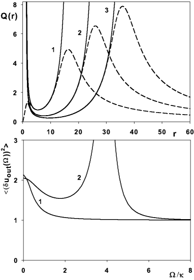
Figure 1: a) The Mandel Q-parameter (21) vs the pump parameter $r$. Dashed line shows results obtained with help of function $P_{0}$ (38). 1) $c=20$; 2) $c=30$; 3) $c=40$. For all curves $I_{s}=20$. b) The spectrum of amplitude fluctuations. 1) $r=r_{m}=199$, 2) $r=3$. For all curves $I_{s}=0.2$, $c=400$.

II.4 2.4 Bad-cavity regime

The considered single-emitter laser relates to so called high $\beta$ lasers - the lasers with high fraction $\beta$ of spontaneous emission into the lasing mode (see expression for $\beta$ in Sec. 3, Eq. (49)). Most of present work on the intensity noise in high $\beta$ lasers has been applied to standard semiconductor laser diodes, embedding quantum wells as gain material. These models predict that if $\beta$ is small, the peak-to-valley difference of the relaxation oscillations is very large and it decreases with increasing $\beta$ Bjork1994 ; Protsenko2001 . However, all these models are based on standard rate equations used in quantum well lasers and very few studies have been carried out in this field when switching from quantum well lasers to quantum dot lasers. Some recent research was focused on the turn-on dynamics and relaxation oscillation in standard quantum dots lasers Ludge2008 but has not been extended to unconventional high $\beta$ nanolasers.

Here we use results obtained in Sec. 2.2 to analyze behaviour of our nanolaser in the case of bad-cavity regime $I_{s}\ll 1$. As was mentioned above, for that we only need to preserve the following condition $cI_{s}\gg 8$.

If the pump rate $r$ is close to the maximum point $r_{m}$ the amplitude fluctuations spectrum is described by the same Eqs. (18, 22) as in a good-cavity regime (see Fig. 1b, curve 1). The main difference is the magnitude of the width $\Omega_{0}$ (19) for the amplitude fluctuations spectrum.

Other situation takes place when the pump rate $r$ lies not far from the threshold point $r_{th}$. In this case the high peak in the amplitude fluctuations spectrum appears (see Fig. 1b, curve 2). The physical origin of this peak is the relaxation oscillation phenomenon. Because of linearization procedure break down in the vicinity of threshold $r_{th}$, we can not correctly define width and height of this peak, but we can estimate the frequency of the relaxation oscillations $\Omega_{osc}/\kappa=I_{s}\sqrt{c(r-1)/2}$.

III 3. MASTER EQUATION APPROACH

This section are devoted to investigation of the nanolaser properties with help of master equation for density matrix. This approach have been used by many authors. Thus in Mu1992 the master equation have been reduced to system of first order, ordinary differential equations and analyzed numerically. In Jones1999 ; Clemens2004 more efficient quantum trajectory algorithm have been developed for numerical evaluating of master equation. The works Kilin2001 ; Kilin2002 are devoted to analysis of the master equation written in terms of coherent states for field. In light of our interest, we want to briefly discuss one of them, namely Kilin2001 . Authors have worked with the system of equations for Glauber-Sudarshan P function and additional quasi-probabilities. Besides numerical simulations they have also found approximated expression for P function which can be used in the case of good-cavity regime. Here we follow the nearest approach as in Kilin2001 , but we manage to derive isolated stationary equation for P function. A detailed analysis of the latter allows us to obtain approximated solution, which has wider region of application than that in Kilin2001 .

III.1 3.1 Coherent state representation of master equation

The master equation for our nanolaser is (see, for example, Clemens2004 )

$$\frac{\partial\hat{\rho}}{\partial t}= - \frac{i}{\hbar}\Bigl{[}\hat{V},\hat{\rho}\Bigr{]}+\frac{\kappa}{2}\left(2\text{ }\hat{a}\hat{\rho}\hat{a}^{{\dagger}}-\hat{a}^{{\dagger}}\hat{a}\hat{\rho}-\hat{\rho}\hat{a}^{{\dagger}}\hat{a}\right)$$ (24)

$$+ \frac{\gamma}{2}\left(2\hat{\sigma}\hat{\rho}\hat{\sigma}^{{\dagger}}-\hat{\sigma}^{{\dagger}}\hat{\sigma}\hat{\rho}-\hat{\rho}\hat{\sigma}^{{\dagger}}\hat{\sigma}\right)$$

$$+ \frac{\Gamma}{2}\left(2\hat{\sigma}^{{\dagger}}\hat{\rho}\hat{\sigma}-\hat{\sigma}\hat{\sigma}^{{\dagger}}\hat{\rho}-\hat{\rho}\hat{\sigma}\hat{\sigma}^{{\dagger}}\right),$$

where interaction between the cavity mode and the single two-level system is given by the Jaynes-Cummings Hamiltonian

$$\hat{V}=i\hbar g\left(\hat{a}^{{\dagger}}\hat{\sigma}-\hat{\sigma}^{{\dagger}}\hat{a}\right).$$ (25)

Finally, we want to obtain equation for P function, for that we need to rewrite Eq. (24) in terms of coherent states for field $|z\rangle$, $|z^{\ast}\rangle$ and in projections of the density operator on the two-level system states $|1\rangle$ and $|2\rangle$. Using well known rules (see, for example, Ref. RulesCoherent )

$$\hat{a}\hat{\rho} \rightarrow z\hat{\rho}\left(z,z^{\ast}\right),$$

$$\hat{\rho}\hat{a} \rightarrow \left[z-\frac{\partial}{\partial z^{\ast}}\right]\hat{\rho}\left(z,z^{\ast}\right),$$

$$\hat{\rho}\hat{a}^{{\dagger}} \rightarrow z^{\ast}\hat{\rho}\left(z,z^{\ast}\right),$$

$$\hat{a}^{{\dagger}}\hat{\rho} \rightarrow \left[z^{\ast}-\frac{\partial}{\partial z}\right]\hat{\rho}\left(z,z^{\ast}\right),$$ (26)

where $z$, $z^{\ast}$ are the complex variables and introduce the following quasi-probabilities $\rho_{ik}\left(z,z^{\ast}\right)=\left\langle i\right|\hat{\rho}\left(z,z^{\ast}\right)\left|k\right\rangle\equiv\rho_{ik}$ ($i,k=1,2$), $D=\rho_{22}\left(z,z^{\ast}\right)-\rho_{11}\left(z,z^{\ast}\right)$ and P function $P=\rho_{11}\left(z,z^{\ast}\right)+\rho_{22}\left(z,z^{\ast}\right)$, we obtain from Eq. (24) the system of partial differential equations

$$\frac{\partial P}{\partial t} = \frac{\partial}{\partial z}\left(\frac{\kappa}{2}zP-g\rho_{21}\right)+\frac{\partial}{\partial z^{\ast}}\left(\frac{\kappa}{2}z^{\ast}P-g\rho_{12}\right),$$

$$\frac{\partial D}{\partial t} = (\Gamma-\gamma)P-(\Gamma+\gamma)D+\frac{\partial}{\partial z}\left(\frac{\kappa}{2}zD+g\rho_{21}\right)$$

$$+ \frac{\partial}{\partial z^{\ast}}\left(\frac{\kappa}{2}z^{\ast}D+g\rho_{12}\right)-2g\left[z^{\ast}\rho_{21}+z\rho_{12}\right],$$

$$\frac{\partial\rho_{21}}{\partial t} = -\frac{\left(\Gamma+\gamma\right)}{2}\rho_{21}+\frac{\partial}{\partial z}\left(\frac{\kappa}{2}z\rho_{21}\right)+\frac{\partial}{\partial z^{\ast}}\left(\frac{\kappa}{2}z^{\ast}\rho_{21}\right)$$ (27)

$$+ g\left[zD-\frac{1}{2}\frac{\partial}{\partial z^{\ast}}\left(P+D\right)\right].$$

The first equation in this system is written in special form which can be associated with conservation law for the quasi-probability $\partial P/\partial t=div\overline{J}$, where $\overline{J}$ is known as probability current density. The additional quasi-probabilities $D$ and $\rho_{21}$ have a clear physical meaning. Thus, the mean values for inversion and polarization of the two-level system are expressed through $D$ and $\rho_{21}$ as $\left\langle\hat{D}\right\rangle=\int D\left(z,z^{\ast}\right)d^{2}z$, $\left\langle\hat{\sigma}\right\rangle=\int\rho_{21}\left(z,z^{\ast}\right)d^{2}z$.

III.2 3.2 Stationary solution

In stationary regime the probability current density $\overline{J}$ can be equated with zero (see, for example, Mandel ; Risken ) what gives the following relations $\rho_{21}=\left(\rho_{12}\right)^{\ast}=\left(\kappa/2g\right)zP$. The latter allows us to eliminate $\rho_{21}$, $\rho_{12}$ from the stationary form of the system (27) and obtain two coupled equations for $P$ and $D$. In the new variables $I=\left|z\right|^{2}$ and $\varphi$ ($z=\sqrt{I}\exp\left(i\varphi\right)$) these equations read

$$IP-\frac{I_{s}}{2}\left[\left(r-1\right)P-\left(r+1\right)D\right]=\frac{1}{2}\frac{\partial}{\partial I}I\left(P+D\right),$$ (28)

$$IP\frac{\left(r+1+1/I_{s}\right)}{c}-\left[ID+\frac{1}{2}\left(P+D\right)\right]$$

$$=\frac{1}{2}\frac{\partial}{\partial I}\left[\frac{4}{cI_{s}}I^{2}P-I\left(P+D\right)\right]-\frac{i}{4}\frac{\partial}{\partial\varphi}\left(P+D\right),$$ (29)

where we introduced above mentioned dimensionless parameters $I_{s}$, $c$, $r$.

There is no phasing influence on our nanolaser, e.g. - external field with fixed phase or coherent pumping. Therefore expected stationary solution does not depend on phase and we can write $P$ and $D$ as only function of $I=\left|z\right|^{2}$. This is also following from the second Eq. (29): the term proportional to imaginary unit should be equated to zero because of reality of functions $P$ and $D$.

Let us derive isolated equation for the P function in the stationary regime. Using Eqs. (28, 29) we can express function $D$ in terms of $P$

$$D=\frac{1}{(r+1-1/I_{s})-2I/I_{s}}\left(\frac{4}{cI_{s}^{2}}I^{2}\frac{\partial}{\partial I}P+\frac{2\left[3-I_{s}\left(r+1+c\right)\right]}{cI_{s}^{2}}IP+(r-1+1/I_{s})P\right).$$ (30)

Now put this relation into the first or the second equation in the system Eqs. (28, 29). In such a way we get isolated equation for $P$ function

$$P^{\prime\prime}\left(I\right)+p(I)P^{\prime}\left(I\right)+q(I)P\left(I\right)=0,$$

$$p(I)=\left(a_{10}+a_{11}I+a_{12}I^{2}\right)/\left(a_{02}I^{2}+a_{03}I^{3}\right),$$

$$q(I)=\left(a_{20}+a_{21}I+a_{22}I^{2}\right)/\left(a_{02}I^{2}+a_{03}I^{3}\right),$$ (31)

where the prime indicates derivative with respect to variable $I=\left|z\right|^{2}$ and functions $p(I)$, $q(I)$ depend on physical parameters $I_{s}$, $c$, $r$ via $a_{ik}$ (see Appendix).

The obtained equation is the second order differential equation with polynomial coefficients. To use this equation we need to define boundary $P(0)$, $P(\infty)$ or "initial" $P\left(0\right)$, $P^{\prime}(0)$ conditions. If we equate the variable $I$ to zero in Eq. (31) we obtain the following relation $P^{\prime}(0)=-a_{20}/a_{10}P\left(0\right)$. This relation together with normalization of the quasi-probability $P$ gives a comfortable way to define the "initial" condition for numerical simulations.

In the case of good-cavity regime functions $p(I)$ and $q(I)$ in Eq. (31) contain large parameters like $cI_{s}$, $I_{s}^{3}$ or $I_{s}^{2}$ (see Appendix). Therefore, we can try to find approximated solution of Eq. (31) using the perturbation method (see, for example, Ref. Nayfeh ). The point of this method is representation of the unknown function $P$ as iterative series $P=\sum_{n=0}^{\infty}\lambda^{-n}P_{n}$, where $\lambda$ is a large parameter. A substitution of the latter series into Eq. (31) with subsequent equating to zero of terms with same powers $1/\lambda$ gives possibility to find the different orders of approximations $P_{n}$.

To isolate the correct single large parameter let us rewrite $p(I)$ and $q(I)$ in the following form

$$p(I)=a_{12}\left(I-I_{-1}\right)\left(I-I_{+1}\right)/I^{2}\left(I-I_{00}\right),$$ (32)

$$q(I)=a_{22}\left(I-I_{-2}\right)\left(I-I_{+2}\right)/I^{2}\left(I-I_{00}\right),$$ (33)

where roots are

$$I_{\pm i}=-a_{i1}/2a_{i2}\pm\sqrt{\left(a_{i1}/a_{i2}\right)^{2}-4a_{i0}/a_{i2}}/2,\\ \text{ }I_{00}=-a_{02}.$$

In the conditions $I_{s}\gg 1$, $c>8$ the magnitudes of the roots $I_{+1}$, $I_{+2}$, $I_{00}$ approximately equal each other and the roots $I_{-1}$, $I_{-2}$ have the similar order. So, it is natural to save all $I_{\pm i}$ and extract the large parameter from the constants $a_{12}$, $a_{22}$ in Eqs. (32, 33). This parameter is therefore $\lambda=cI_{s}\left(=a_{22}\approx-a_{12}\right)$ and Eq. (31) can be written as follows

$$\lambda^{-1}P^{\prime\prime}\left(I\right)+\tilde{p}(I)P^{\prime}\left(I\right)+\tilde{q}(I)P\left(I\right)=0,$$ (34)

where $\tilde{p}(I)=p(I)/a_{22}$, $\tilde{q}(I)=q(I)/a_{22}$. Here we want to note that we do not neglect the term $r/c$ in relation $a_{12}/a_{22}=\left(7-3I_{s}(r+1)-2cI_{s}\right)/2cI_{s}$, because of pump rate $r$ can be comparable or bigger than $c$ (for example near to maximum $r_{m}$ or to quenching $r_{q}$ points).

Thus, in zero-order approximation (first term in the series $P=\sum_{n=0}^{\infty}\lambda^{-n}P_{n}$) we neglect the term in Eq. (34) proportional to $1/\lambda$ what implies first-order differential equation for function $P_{0}$

$$a_{12}\left(I-I_{-1}\right)\left(I-I_{+1}\right)P_{0}^{\prime}\left(I\right)$$

$$+ a_{22}\left(I-I_{-2}\right)\left(I-I_{+2}\right)P_{0}\left(I\right)=0.$$ (35)

$P_{0}$ is then found from Eq. (35):

$$P_{0}\left(I\right)=\left\{\begin{array}[]{cc}N_{0}\left(1-I/I_{-1}\right)^{f_{1}}\left(1-I/I_{+1}\right)^{f_{2}}\exp\left(-\frac{a_{22}}{a_{12}}I\right),&\text{if}\text{ }I\leq I_{-1}\\ 0,&\text{otherwise}\end{array}\right.\,$$ (38)

$$f_{1}=-\frac{a_{22}}{a_{12}}\frac{\left(I_{-1}-I_{-2}\right)\left(I_{-1}-I_{+2}\right)}{\left(I_{-1}-I_{+1}\right)},\text{ }f_{2}=\frac{a_{22}}{a_{12}}\frac{\left(I_{+1}-I_{-2}\right)\left(I_{+1}-I_{+2}\right)}{\left(I_{-1}-I_{+1}\right)},$$

where $N_{0}$ is normalizing constant. The roots and consequently the powers $f_{1}$, $f_{2}$ in Eq. (38) have complex structure and will be estimated below in some special cases.

To understand why our solution is restricted we note that the roots $I_{\pm 1}$ of function $p(I)$ in Eq. (31) are known as turning points, where oscillating behaviour of $P\left(I\right)$ can change on exponential. A careful examination of Eq. (31) shows that in the conditions $I_{s}\gg 1$, $c>8$ on the $I$-domain ranging from $0$ to turning point $I_{-1}$ the $P\left(I\right)$ is positive and nonoscillating function. Moreover, its essential changing occurs just on latter domain (it is not for every set of parameters $r$, $I_{s}$, $c$, see below). Otherwise, when $I>I_{-1}$ then $P\left(I\right)$ becomes oscillating function. The obtained solution Eq. (38) can not describe any oscillations, moreover it possesses imaginary values when $I>I_{-1}$, therefore we have restricted definition domain for our solution by the value $I_{-1}$ and call them boundary root.

To reveal physical meaning of the boundary root we have simplified expression for $I_{-1}$ and found maximum of function $P_{0}\left(I\right)$ on the domain $\left(0,I_{-1}\right)$. When $I_{s}\gg 1$, $c>8$ we have managed to estimate the latter quantities with help of results obtained in Sec. 2.3: $I_{-1}\approx I_{s}r/\left(2+3r/c\right)\geq I_{0}\left[1+Q\left(r,c\right)\right]$ and the point where $P_{0}\left(I\right)$ reaches his maximum is $I=I_{-2}\approx I_{0}$. Thus, P function has a maximum at the point corresponding to the semiclassical intensity $I_{0}$ Eq. (4) and the boundary root is at a distance $I_{0}Q\left(r,c\right)$ from it, where $Q\left(r,c\right)$ is the Mandel Q-parameter Eq. (21).

In the Fig. 2 we plot the P function calculated using Eq. (38) (dashed line) and using numerical simulations of the equation (31) (solid gray line). The different curves correspond to different values of pump rate $r$ while $c$ and $I_{s}$ are fixed. We see a very good agreement with numerical results.

The main divergency appears for value of pump rate discovered in Sec. 2.3, namely for $r=c/5$, where the Mandel Q-parameter $Q\left(r,c\right)$ (21) has a minimum (see Eq. (20) and text below). In the right wing of P function (Fig. 2b) the small oscillations appear when $c$ becomes comparable with $I_{s}$, but still our solution is good. With growing of $c$ the oscillations become more pronounced and the maximum of P function goes out of domain $\left(0,I_{-1}\right)$ and our solution (38) becomes inapplicable in vicinity of $r=c/5$. It is interesting to note that critical situation occurs when $c\geqslant 200$. For latter values of $c$ and for arbitrary saturation intensity $I_{s}$ the maximum of P function goes out of the domain $\left(0,I_{-1}\right)$. As mentioned above, the P function acquires oscillating character for $I>I_{-1}$, what probably indicates on the nonclassical effect associated with photon antibunching.

Now let us analyze the obtained solution (38) in some special cases.

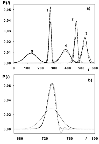
Figure 2: a) P function vs $I=\left|z\right|^{2}$ for different pump parameter $r$. 1) $r=8$, 2) $r=16$, 3) $r=24$, 4) $r=36$, 5) $r=44$. For all curves $I_{s}=100$, $c=50$; b) Oscillation behaviour of the P function, $I_{s}=c=100$, $r=c/5=20$. Dashed line - solution (38), solid gray line - numerical simulation, dotted line - solution from Ref. Kilin2001 .

III.2.1 Far below threshold and far above quenching

At first we consider situation when the pump rate lies far below threshold $r\ll r_{th}$. In this case the average value of $I=\left|z\right|^{2}$ is small and the following inequalities $I/I_{-1}\approx I/\left(I_{s}r/2\right)\ll 1$, $I/I_{+1}\approx I/(I_{s}\left(r+1\right)/2)\ll 1$ are satisfied. Thus, the factor in front of exponential in Eq. (38) can be approximated as follows

$$\left(1-I/I_{-1}\right)^{f_{1}}\left(1-I/I_{+1}\right)^{f_{2}}$$

$$=\exp\left[f_{1}\ln\left(1-I/I_{-1}\right)\right]\exp\left[f_{2}\ln\left(1-I/I_{+1}\right)\right]$$

$$\approx\exp\left[-\left(f_{1}/I_{-1}+f_{2}/I_{+1}\right)I\right].$$ (39)

The $P_{0}$ is therefore

$$P_{0}\left(I\right)=\frac{1}{\left(a_{10}/a_{20}\right)}\exp\left(-\frac{I}{\left(a_{10}/a_{20}\right)}\right).$$ (40)

The obtained expression for P function corresponds to thermal distribution with the following mean number of photons in the cavity $\left\langle\hat{n}\right\rangle=a_{10}/a_{20}\sim r$.

For the values of pump rate lying far above quenching point $r\gg r_{q}$ we can make the same manipulation with Eq. (38) as above. Using inequalities $I/I_{-1}\approx I/(I_{s}r/\left(2+3r/c\right))\ll 1$, $I/I_{+1}\approx I/(I_{s}r/2)\ll 1$ which occur in this case, we get the same thermal distribution as Eq. (40), but the mean number of photons possesses another behaviour $\left\langle\hat{n}\right\rangle=a_{10}/a_{20}\sim 1/r$.

In the two limiting situations, when $r\rightarrow 0$ or $r\rightarrow\infty$, the corresponding mean number of photons converge to zero and the distribution Eq. (40) gives Dirac delta-function $P_{0}\left(I\right)=\delta\left(I\right)$, what coincides with the thermal distribution with zero temperature.

III.2.2 Near to maximum point $r_{m}$

Here we consider situation when the pump rate is in the vicinity of $r_{m}$, where the semiclassical solution $I_{0}$ Eq. (4) reaches his maximum. In this case the powers in Eq. (38) are simplified as $f_{1}\approx I_{s}\left(3\left(r+1\right)^{3}+2c^{2}-c\left(r+1\right)\left(r-5\right)\right)/\left(3\left(r+1\right)+2c\right)^{2}$, $f_{2}\approx 0$ and the root $I_{-2}$ becomes similar to $I_{0}$. Simple algebra leads to following expression for $P_{0}$

$$P_{0}\left(\Delta I\right)=\left\{\begin{array}[]{cc}N_{0}\left[\left(1-\Delta I/\Lambda\right)^{\Lambda}\exp\left(\Delta I\right)\right]^{\alpha},&\text{if}\text{ }\Delta I\leqslant\Lambda\\ 0,&\text{otherwise}\end{array}\right.\$$ (43)

(44)

where we introduced new variable $\Delta I=I-I_{0}$ and constants $\Lambda=f_{1}/\alpha$, $\alpha=2c/\left(3\left(r+1\right)+2c\right)$. For chosen values of pump rate the average value of $\Delta I$ is small and the inequality $\Delta I/\Lambda\ll 1$ is satisfied. Thus for the factor in front of exponential in Eq. (44) we can write

$$\left(1-\Delta I/\Lambda\right)^{\Lambda} = \exp\left[\Lambda\ln\left(1-\Delta I/\Lambda\right)\right]$$ (45)

$$\approx \exp\left[-\Delta I-\Delta I^{2}/2\Lambda\right],$$

what implies Gaussian P function

$$P_{0}\left(I\right)=N_{0}\exp\left[-\frac{\left(I-I_{0}\right)^{2}}{2\Lambda/\alpha}\right].$$ (46)

Here we removed the restriction on $P_{0}$. Indeed, the distribution (46) never really sees the boundary and $I$ can be taken to run from $0$ to $\infty$.

Using the obtained Eq. (46) we can estimate the average value of photons in the cavity $\left\langle\hat{n}\right\rangle$ and its variance $\langle\left(\Delta\hat{n}\right)^{2}\rangle$

$$\left\langle\hat{n}\right\rangle = \int_{0}^{\infty}IP_{0}\left(I\right)dI\approx I_{0},$$ (47)

$$\langle\left(\Delta\hat{n}\right)^{2}\rangle = \left\langle\hat{n}\right\rangle+\int_{0}^{\infty}\left(I-\left\langle\hat{n}\right\rangle\right)^{2}P_{0}\left(I\right)dI$$ (48)

$$\approx I_{0}\left[1+\Lambda/\left(\alpha I_{0}\right)\right].$$

A substitution of the explicit form of $\Lambda$ and $\alpha$ into the expression for variance gives $\langle\left(\Delta\hat{n}\right)^{2}\rangle=I_{0}\left[1+Q\left(r,c\right)\right]$, where $Q\left(r,c\right)$ is the Mandel Q-parameter obtained from linear theory (21).

In the weak coupling regime $c<I_{s}$ the obtained Eq. (46) works good for values of pump rate lying in whole semiclassical region $r_{th}<r<r_{q}$. In the strong coupling regime $c>I_{s}$ the symmetrical Gaussian distribution (46) is not sufficient and it becomes more pronounced near to mentioned value of pump rate $r=c/5$.

III.2.3 Threshold

In our previous report Larionov2011 we considered nanolaser behaviour around the semiclassical threshold $r_{th}$ (5) and specified the condition required for thresholdless regime. Here we continue our research using the obtained Eq. (38).

The behaviour of P function in the threshold point $r_{th}$ for three different regimes 1) $c\ll I_{s}$, 2) $c\approx I_{s}$, 3) $c\gg I_{s}$ is shown in Fig. 3a. To realize these regimes we fix the large coupling constant $c=100$ and set the different values of the saturation intensity: $I_{s}=600$, $60$, $6$ (we choose such values of $I_{s}$ for better resolution of P function behaviour). In the weak coupling regime ($c\ll I_{s}$) the P function has a typical plateau (it is marked by solid straight line, curve 1), which indicates transition to lasing: from thermal to Gaussian type distribution. As saturation intensity is decreased and the strong coupling regime ($c\gg I_{s}$) occurs the maximum of P function moves from zero value of variable $I$ and the semiclassical threshold behaviour disappears (curve 3).

Above we obtained the maximum point for $P_{0}$ (38) and it was the root $I_{-2}$. To define the threshold value of pump rate we need to solve equation $I_{-2}\left(r\right)=0$, i.e. find such value of $r$ when the maximum of the P function is in the point $I=I_{-2}\left(r\right)=0$. The approximate solution is $\tilde{r}=1+4/c-2/I_{s}$. When $c\ll I_{s}$ then the last term can be neglected and $\tilde{r}$ equal to semiclassical threshold $r_{th}\approx 1+4/c>1$ (5). When $c\gg I_{s}$ then $\tilde{r}$ becomes smaller than unity what indicates the disappearance of the semiclassical threshold and transition to thresholdless regime (see the vanishing of narrow peak in the behaviour of Mandel Q parameter in our previews report Larionov2011 , Fig. 2). The dynamics of $\tilde{r}$ in above three considered regimes is $\tilde{r}\approx 1.04$, $1$, $0.66$ (remind that $r_{th}=1.04$).

At the end of this section we want to correct the misprint occurred in our previous report (see formula (13) in Larionov2011 ). The valid expression for fraction $\beta$ of spontaneous emission into the laser mode is

$$\beta=c/\left[\left(c+1\right)+I_{s}\left(r+1\right)\right].$$ (49)

We should note that this misprint did not affect on all our results and discussions.

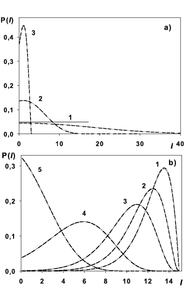
Figure 3: P function vs $I=\left|z\right|^{2}$. a) Transition to the thresholdless regime. 1) $I_{s}=600$, 2) $I_{s}=60$, 3) $I_{s}=6$. For all curves $c=100$, $r=r_{th}=1.04$. b) Parameters was taken as in Ref. Kilin2001 : 1) $c=2000$, $I_{s}=5$, $r=6$, 2) $c=1428.57$, $I_{s}=7$, $r=4.28$, 3) $c=1000$, $I_{s}=10$, $r=3$, 4) $c=500$, $I_{s}=20$, $r=1.5$, 5) $c=285.7$, $I_{s}=35$, $r=0.86$. Dashed line - solution (38), solid gray line - numerical simulation, dotted line - solution from Ref. Kilin2001 .

III.2.4 Comparing with other authors

In introduction to this section we mentioned that close approach based on quasi-probabilities have been considered by two authors Karlovich and Kilin in Kilin2001 . They have worked with first order differential equation system for function P and additional quasi-probabilities. By neglecting of small parameters in this system they have obtained integrable equations and as a result the analytical formula for P function. The structure of their solution has an identical form with our Eq. (38) (see formula (9) in Kilin2001 ), but this solution works good in the region near to semiclassical threshold $r_{th}$ or quenching points $r_{q}$. For the pump rate lying around the maximum point $r_{m}$ it gives uncorrect result for width of function $P$ and as a consequence the uncorrect variance of the photon distribution.

In the Fig. 3b we plot some graphics of quasi-probability P for parameters taken from Kilin2001 . It is clear to see that our Eq. (38) gives the same result as a solution (9) obtained in Kilin2001 and all of them are in a good agreement with numerical simulations. The Fig. 2a,b demonstrate that for the pump rate lying around the maximum point $r_{m}$ our Eq. (38) (dashed line) has an advantage with (9) Kilin2001 (dotted line). The latter indicates well the maximum of true P function, but the width is uncorrect.

The derivation of a single equation for P function (31) and accurate extraction of large parameters gives us possibility to obtained the solution which has more wide region of application.

IV 4. SUMMARY

In this paper we have studied physical properties of a single-emitter laser. The problem have been investigated in terms of the Heisenberg-Langevin equations and in terms of the master equation for density matrix. In both approaches we have provided analytical results which are summarized below.

In the case of good-cavity regime with help of the Heisenberg-Langevin approach we have obtained analytical expressions for linewidth Eq. (23), amplitude fluctuation spectrum Eq. (18) and Mandel Q parameter Eq. (21). These results work good in the semiclassical region of pumping rate $r_{th}<r<r_{q}$. According to nanolaser behaviour the latter region can be split into two subregions. In the first subregion $r<r_{m}$ the nanolaser behaviour is similar to that of conventional laser. Also in this subregion for $r$ centered around $r=c/5$ and for large coupling constant ($c\geqslant 200$) we have discovered the small noise reduction below the SQL in the laser light outside the cavity and small negative values in $Q\left(r,c\right)$ (21). The master equation approach confirms this nonclassical phenomenon: P function manifests oscillating behaviour. Probably, these negative values are the result of the well-known antibunching phenomenon for a single-emitter. In the second subregion $r>r_{m}$ the excess noise is always takes place. The P function in this subregion does not have any nonclassical features.

In the bad-cavity regime we have observed two different situations: when the pump rate $r$ is close to its maximum value $r_{m}$ then laser generates as in the good-cavity regime; when $r$ is close to threshold $r_{th}$ then high peak in the amplitude fluctuations spectrum appears which indicates on the relaxation oscillation phenomenon.

With the help of the master equation for density matrix written in terms of coherent states we have managed to derive the stationary equation for the Glauber-Sudarshan P function (31). A detailed analysis of this equation allowed us to obtain approximated solution Eq. (38), which works good when $cI_{s}\gg 1$. We have analyzed Eq. (38) in some special cases. In the good-cavity regime in the semiclassical region $r_{th}<r<r_{q}$ Eq. (38) can be written as Gaussian distribution with mean value coincides with the semiclassical intracavity intensity $I_{0}$ (4) and with width $I_{0}Q\left(r,c\right)$ (21). For the values of pump rate lying far below threshold and far above self-quenching points Eq. (38) corresponds to thermal distribution.

Using Eq. (38) we have also obtained approximated expression for threshold pump rate $\tilde{r}=1+4/c-2/I_{s}$. In the weak-coupling regime ($I_{s}\gg c$) the last term can be neglected what implies the semiclassical threshold $\tilde{r}=r_{th}\approx 1+4/c$. When strong-coupling regime ($I_{s}\ll c$) occurs then $\tilde{r}<r_{th}$ what indicates on the transition to thresholdless regime.

V Acknowledgments

This work was supported by French National Agency (ANR) through Nanoscience and Nanotechnology Program (Project NATIF n^∘ANR-09-NANO-012-01), by the CNRS-RFBR collaboration (CNRS 6054 and RFBR 12-02-91056) and by external fellowship of the Russian Quantum Center (Ref. number 86).

VI Appendix

The constants $a_{ik}$ in Eq. (31)

$$a_{02} = \frac{1}{2}-I_{s}\frac{\left(r+1\right)}{2},$$

$$a_{03} = 1,$$

$$a_{10} = I_{s}^{2}\frac{cr}{4}-I_{s}^{3}\frac{cr(r+1)}{4},$$

$$a_{11} = \frac{9}{4}-I_{s}\frac{6(r+1)+c}{2}+I_{s}^{2}\frac{3(r+1)^{2}+c(4r+2)}{4},$$

$$a_{12} = \frac{7}{2}-I_{s}\frac{3(r+1)+2c}{2},$$

$$a_{20} = \frac{3}{2}-I_{s}\frac{11(r+1)+3c}{4}+I_{s}^{2}\frac{3(r+1)^{2}+2c}{2}$$

$$+ I_{s}^{3}\frac{c(r+1)}{4}\left[(r-1)-\frac{(r+1)^{2}}{c}\right],$$

$$a_{21} = \frac{3}{2}-2I_{s}(r+1)-I_{s}^{2}\frac{2cr-(r+1)^{2}}{2},$$

$$a_{22} = cI_{s}.$$ (50)

References

- (1) Yi Mu, C. M. Savage, Phys. Rev. A. 46, 9, 5944 (1992).
- (2) C. Ginzel, H.-J. Briegel, U. Martini, B.-G. Englert, and A. Schenzle, Phys. Rev. A 48 732 (1993).
- (3) T. Pellizzari and H. Ritsch, Phys. Rev. Lett. 72, 3973 (1994).
- (4) M. Loffler, G. M. Meyer, and H. Walther, Phys. Rev. A 55, 3923 (1997).
- (5) B. Jones, S. Ghose, J. P. Clemens, P. R. Rice, and L. M. Pedrotti, Phys. Rev. A 60 3267 (1999).
- (6) T. B. Karlovich and S. Ya. Kilin, Opt. Spectr. 91, 343 (2001).
- (7) S. Ya. Kilin and T. B. Karlovich, J. Exp. Theor. Phys. 95, 805 (2002).
- (8) S. Ya. Kilin and A. B. Mikhalychev, Phys. Rev. A 85, 063817 (2012).
- (9) J. P. Clemens, P. R. Rice, and L. M. Pedrotti, J. Opt. Soc. Am. B 21, 2025 (2004).
- (10) J. McKeever, A. Boca, A. D. Boozer, J. R. Buck, and H. J. Kimble, Nature 425, 268 (2003).
- (11) F. Dubin, C. Russo, H. G. Barros A. Stute, C. Becher, P. O. Schmidt, and R. Blatt, Nature Physics 6, 350 (2010).
- (12) M. Nomura, N. Kumagai, S. Iwamoto, Y. Ota, and Y. Arakawa, Opt. Express 17, 15975 (2009).
- (13) N. V. Larionov, M. I. Kolobov, Phys. Rev. A, 84, 055801 (2011).
- (14) M. Lax, in Statistical Physics, Phase Transitions and Superconductivity, edited by M. Chretien, E. P. Gross, and S. Dreser (Gordon and Breach, New York, 1968), Vol. II, p. 425; W. H. Louisell, Quantum Statistical Properties of Radiation (Wiley, New York, 1973);
- (15) C. W. Gardiner and P. Zoller, Quantum Noise (Springer, Berlin, 2000).
- (16) M. I. Kolobov, L. Davidovich, E. Giacobino, and C. Fabre, Phys. Rev. A 47, 1431 (1993).
- (17) F. Haake, M. I. Kolobov, and C. Seeger, Phys. Rev. A 54, 1625–1637 (1996).
- (18) J. Y. Courtois, A. Smith, C. Fabre, and S. Reynaud, J. Mod. Phys. 38, 177 (1991).
- (19) G. Bjork, A. Karlsson and Y. Yamamoto, Phys. Rev. A 50, 1675 (1994).
- (20) I. E. Protsenko and M. Travagnin, Phys. Rev. A 65, 013801 (2001).
- (21) K. Ludge, M. J. P. Moritz, E. Malic, P. Hovel, M. Kuntz, D. Bimberg, A. Knorr and E. Scholl, Phys. Rev. B 78, 035316 (2008).
- (22) Scully O. Zubairy M. S. Quantum optics, (Cambridge University Press, 1997).
- (23) L. Mandel, E. Wolf, Optical Coherence and Quantum Optics, (Cambridge University Press, 1995).
- (24) H. Risken, The Fokker-Planck equation, (Spring-Verlag Berlin Heidelberg, 1989).
- (25) Ali H. Nayfeh, Perturbation methods, (John Wiley & Sons, 1973).