Giant radio relics in galaxy clusters: reacceleration of fossil relativistic electrons?

Abstract

Many bright radio relics in the outskirts of galaxy clusters have low inferred Mach numbers, defying expectations from shock acceleration theory and heliospheric observations that the injection efficiency of relativistic particles plummets at low Mach numbers. With a suite of cosmological simulations, we follow the diffusive shock acceleration as well as radiative and Coulomb cooling of cosmic ray electrons during the assembly of a cluster. We find a substantial population of fossil electrons. When reaccelerated at a shock (through diffusive shock acceleration), they are competitive with direct injection at strong shocks and overwhelmingly dominate by many orders of magnitude at weak shocks, $\mathcal{M}\lower 2.15277pt\hbox{$\;\buildrel<\over{\sim}\;$}3$, which are the vast majority at the cluster periphery. Their relative importance depends on cooling physics and is robust to the shock acceleration model used. While the abundance of fossils can vary by a factor of $\sim 10$, the typical reaccelerated fossil population has radio brightness in excellent agreement with observations. Fossil electrons with $1\lower 2.15277pt\hbox{$\;\buildrel<\over{\sim}\;$}\gamma\lower 2.15277pt\hbox{$\;\buildrel<\over{\sim}\;$}100$ ($10\lower 2.15277pt\hbox{$\;\buildrel<\over{\sim}\;$}\gamma\lower 2.15277pt\hbox{$\;\buildrel<\over{\sim}\;$}10^{4}$) provide the main seeds for reacceleration at strong (weak) shocks; we show that these are well-resolved by our simulation. We construct a simple self-similar analytic model which assumes steady recent injection and cooling. It agrees well with our simulations, allowing rapid estimates and physical insight into the shape of the distribution function. We predict that LOFAR should find many more bright steep-spectrum radio relics, which are inconsistent with direct injection. A failure to take fossil cosmic ray electrons into account will lead to erroneous conclusions about the nature of particle acceleration at weak shocks; they arise from well-understood physical processes and cannot be ignored.

1 Introduction

Diffuse radio emission in clusters falls into two broad classes: smooth, centrally located and unpolarized radio halos (Ferrari et al., 2008, and references therein), and elongated, significantly polarized and steep spectrum radio relics which are seen at cluster outskirts (Kempner et al., 2004, and references therein). The radio halos come in two distinct classes: mini-halos in cool core clusters and giant halos associated with merging clusters. Similar to the radio halos, the radio relics are thought to come in distinct classes which are all associated with merging clusters: fossil radio lobes blown in the past by active galactic nuclei (AGN), which may have been re-energized by compression (radio phoenix; Enßlin & Gopal-Krishna, 2001), and those produced by direct diffusive particle acceleration at accretion/merger shocks (radio gischt; Ensslin et al., 1998; Miniati et al., 2001). Many radio relics have now been seen ($\sim 50$; for recent compilations, see Feretti et al., 2012; Nuza et al., 2012) and the number could increase dramatically with upcoming low frequency radio surveys proposed for the Low Frequency Array (LOFAR), the Westerbork Synthesis Radio Telescope (WSRT), and farther in the future, Square Kilometer Array (SKA). Using numerical simulations combined with a semi-analytic model for radio emission calibrated to existing number counts, Nuza et al. (2012) estimate that LOFAR and WSRT could discover $\sim 2500$ relics and $\sim 900$ relics respectively. The time is therefore ripe to understand how we can best mine these future surveys.

In this paper, we focus on radio gischt, which trace structure formation shock waves. They therefore can illuminate the nature of cosmic accretion/mergers, as well as shock amplification of large-scale magnetic fields (Pfrommer et al., 2008; Pfrommer, 2008; Hoeft et al., 2008; Battaglia et al., 2009; Skillman et al., 2011). Perhaps even more importantly, they allow us to probe in detail the efficiency of shock acceleration in a diffuse, low Mach number ($\mathcal{M}\sim 2-4$) regime, far different from the high Mach number regimes probed in our Galaxy and supernova remnants. Whilst this remains poorly understood, at face value the observations seem to suggest an electron acceleration efficiency significantly in excess of naive theoretical expectations.

A recent spectacular example of radio gischt is CIZA J2242.8+5301, the ‘sausage relic’ (van Weeren et al., 2010), a large ($\sim 2$ Mpc long; located $\sim 1.5$ Mpc from the cluster center) double radio relic system. The post-shock radio spectral index was used to infer the particle spectral slope and hence the shock compression ratio and Mach number ($\mathcal{M}\sim 4.6$), while the decrease in the spectral index (from $\sim 0.6$ to $\sim 2.0$ across the relic’s narrow $\sim 55$ kpc width) toward the cluster center—spectral aging due to synchrotron and inverse Compton losses—was used to infer magnetic field strengths of $\sim 5\,\mu$G. The strong ($\sim 50-60$ per cent) polarization can be attributed to magnetic field frozen into the compressed intracluster medium (ICM), which has been aligned parallel to the shock. The properties of this and similar systems are distinct from fossil radio plasma, which are smaller, have curved, steeper spectra (due to aging), and lobe- or torus-like morphology (e.g., Enßlin & Brüggen, 2002; Pfrommer & Jones, 2011). The power-law spectral index, spectral gradient, and enormous extent clearly support a diffusive shock acceleration (DSA) origin. While turbulent acceleration may be a viable mechanism for energizing CRes in radio halos, it is less plausible for radio relics because of the long acceleration time scales (exceeding several 100 Myrs). The coincidence of radio relic emission with X-ray determined shock fronts over scales of several Mpc imply the injection or reacceleration of CRes on very short timescales that preclude turbulent reacceleration. Otherwise, for instance, for an acceleration timescale of $t_{\rm accel}\sim 3\times 10^{8}$yr and a postshock velocity of $\sim 1000/4\sim 250\,{\rm km\,s^{-1}}$, the radio emission and the shock front would be separated by $\sim 100$ kpc. In addition, turbulent reacceleration models produce curved spectra, which are not seen in radio relics.

However, this then presents a puzzle. Cosmological simulations show that while gas initially undergoes strong shocks (up to $\mathcal{M}\sim 10^{3}$) accreting onto non-linear structures and filaments, shocks in the ICM and cluster outskirts are relatively modest ($\mathcal{M}\sim 1-4$), since the gas has already reached sub-keV temperatures (Ryu et al., 2003; Pfrommer et al., 2006; Skillman et al., 2008; Vazza et al., 2009; Vazza et al., 2011). While DSA is efficient in accelerating particles in the thermal Maxwellian tail at high Mach numbers (Bell, 1978b; Drury, 1983b), and as confirmed in observations of supernova remnants (Parizot et al., 2006; Reynolds, 2008), at lower Mach numbers the efficiency of DSA is known to plummet exponentially. Indeed, in the test-particle regime where suprathermal particles undergo acceleration via a thermal leakage process (which compare well against kinetic DSA simulations) the acceleration efficiency for weak shocks $\mathcal{M}\lesssim 3$ is extremely small; the fraction of protons accelerated is $\sim 10^{-4}-10^{-3}$, and cosmic ray proton (CRp) pressure is $\lower 2.15277pt\hbox{$\;\buildrel<\over{\sim}\;$}1$ per cent of the shock ram pressure (Kang & Ryu, 2011). The acceleration efficiency of electrons at low Mach numbers is likely to be far smaller still. The injection problem for thermal electrons is already known to be severe at high Mach numbers, due to the smaller gyroradius of thermal electrons: the relative acceleration efficiency of cosmic ray electrons (CRes) is lower by $\sim 10^{-2}$ as in the Galaxy (Schlickeiser, 2002) or even $\sim 10^{-4}$ as in supernova remnants (Morlino et al., 2009). These relative efficiencies likely plummets further at low Mach numbers, as is also suggested by heliospheric observations (see §7). These considerations appear to contradict the appearance of bright radio relics, and perhaps suggest that our understanding of DSA at low Mach numbers is incomplete (for recent progress, see Gargaté & Spitkovsky, 2012).

A possible solution is if there is a pre-existing population of CRes with gyroradii comparable or larger than that of the shock thickness. In this case, injection from the thermal pool is no longer an issue (Ensslin et al., 1998; Markevitch et al., 2005; Giacintucci et al., 2008; Kang & Ryu, 2011; Kang et al., 2012). DSA has a much larger effect on radio emission than adiabatic compression; including the downstream magnetic field amplification, synchrotron emission from fossil electrons could be boosted by a factor $\sim 100-1000$ for $\mathcal{M}\sim 3$ (Kang & Ryu, 2011). Thus, the luminosity function of radio gischt will be strongly modified by the presence or absence of a seed relativistic electron population, whose existence has never been directly demonstrated. Note that secondary CRe which arise from hadronic interactions of CRp are not thought to be significant at these low densities, though for a dissenting view, see Keshet (2010). In this paper, we use our existing high-resolution SPH simulations of CRps in clusters (Pinzke & Pfrommer, 2010) to infer whether structure formation shocks could generate them. Note that DSA operates identically on relativistic particles of the same rigidity ($R=Pc/Ze$), so the injected proton and electron spectrum are the same, modulo their relative acceleration efficiency, which we calibrate off Galactic observations.

The main difference is that unlike protons, relativistic electrons can still undergo significant Coulomb and inverse Compton losses in the cluster outskirts. In Fig. 1, we show the cooling time of CRes for difference densities and cosmological epochs. CRes of energy $\sim 10$ GeV that are responsible for $\sim$ GHz emission in a $\mu$G field have energy loss timescales of $\sim 10^{8}$yr at $z=0$ (and cool even more quickly at higher redshift). However, lower energy CRe could potentially survive to be reaccelerated since CRes with momentum $P=(10-100)\,m_{\mathrm{e}}\,c$ have $t_{\rm cool}>t_{\rm H}$ in gas with number densities $n_{\rm e}\leq 3\times 10^{-5}\,\mathrm{cm}^{-3}$ (typical of cluster outskirts) at $z=0$. We evolve the time-dependent cosmic ray (CR) energy equation to track the evolving distribution function of CRe electrons under the combined influence of injection and cooling. We find that the fossil electron population is substantial, and that reacceleration of this population is competitive with direct injection for strong shocks, and will overwhelming dominate radio emission for weak shocks with Mach numbers ${\mathcal{M}}<4$. Since the latter constitute the vast majority of shocks in the cluster periphery, reacceleration is a crucial mechanism which cannot be ignored.

Figure 1: Cooling time of CR electrons for typical conditions in the ICM. CRes can be long-lived if they are injected at low density and at late times. Electrons with kinetic energy $E\simeq p\,m_{\mathrm{e}}c^{2}\simeq 10$ MeV should be the most long-lived in cluster outskirts ($n_{\mathrm{e}}\sim 3\times 10^{-5}\mathrm{cm}^{-3}$) because this energy range maximizes the Coulomb and inverse Compton (IC) cooling times.

The outline of this paper is as follows. In §2, we describe our CR formalism and computational method. In §3, we present results for the fossil electron spectrum, and an analytic model for understanding its essential features. In §4, we study how the fossil population is transformed by a shock, time-resolution effects, and our principal result, that reacceleration dominates direct injection. In §5, we study how the fossil spectrum varies with the shock acceleration model and between clusters. In §6, we discuss observational consequences, including the brightness of relics as a function of Mach number and the relic luminosity function. In §7, we discuss insights gained from heliospheric observations on our adopted shock physics as well as possible limitations of our numerical method. We conclude in §8. Three appendices also spell out various technical points about the cooling and injection process.

2 Fossil Electrons: Method

Our simulations adopt a $\Lambda$CDM cosmology with parameters: $\Omega_{\rm m}=\Omega_{\rm DM}+\Omega_{\rm b}=0.3,\,\Omega_{\rm b}=0.039,\,\Omega_{\Lambda}=0.7,\,h=0.7,\,n_{\rm s}=1$, and $\sigma_{8}=0.9$. The simulations were carried out with an updated and extended version of the distributed-memory parallel TreeSPH code GADGET-2 (Springel, 2005; Springel et al., 2001). Gravitational forces are computed using a combination of particle-mesh and tree algorithms. Hydrodynamic forces are computed with a variant of the smoothed particle hydrodynamics (SPH) algorithm that conserves energy and entropy where appropriate, i.e. outside of shocked regions (Springel & Hernquist, 2002). Our simulations follow the radiative cooling of the gas, star formation, supernova feedback, and a photo-ionizing background (details can be found in Pfrommer et al., 2007). We model the CR physics in a self-consistent way (Pfrommer et al., 2006; Enßlin et al., 2007; Jubelgas et al., 2008) and attach a CRp distribution function to each SPH fluid element. We include adiabatic CRp transport process such as compression and rarefaction, and a number of physical source and sink terms which modify the CRp pressure of each CRp population separately. The main source of injection is diffusive shock acceleration (DSA) at cosmological structure formation shocks, while the primary CRp sinks are thermalization by Coulomb interactions, and catastrophic losses by hadronization. We do not consider CRps injected by supernovae remnants or AGN feedback; these sources should be relatively subdominant in the cluster outskirts. In addition, we neglect the reacceleration of CRp. Firstly, the CRp do not affect radio emission, and hence are unimportant for our study. Secondly, in any case, the CRp population barely cools; only adiabatic cooling (which is an order unity effect) is significant. Reacceleration is only important in counteracting the effects of cooling; otherwise, the effect of the predominantly weak shocks which produce reacceleration on the hard power law of a strong shock is negligible.

Table 1: Cluster sample.

Sim.’s	State(1)	$M_{200}^{(2)}$	$R_{200}^{(2)}$	$kT_{\rm 200}^{(3)}$	$\Delta t,\frac{a_{2}}{a_{1}}$(4)
		[$\mathrm{M}_{\odot}$]	[Mpc]	[keV]
g8a	CC	$2.6\times 10^{15}$	2.9	13.1	1.127
g1a	CC	$1.9\times 10^{15}$	2.5	10.6	1.127
g72a	PostM	$1.6\times 10^{15}$	2.4	9.4	100 Myr
g51	CC	$1.5\times 10^{15}$	2.4	9.4	1.127
g1b	M	$5.2\times 10^{14}$	1.7	4.7	1.127
g72b	M	$2.2\times 10^{14}$	1.2	2.4	100 Myr
g1c	M	$2.0\times 10^{14}$	1.2	2.3	1.127
g8b	M	$1.5\times 10^{14}$	1.1	1.9	1.127
g1d	M	$1.3\times 10^{14}$	1.0	1.7	1.127
g676	CC	$1.3\times 10^{14}$	1.0	1.7	1.049
g914	CC	$1.2\times 10^{14}$	1.0	1.6	1.049
g1e	M	$9.1\times 10^{13}$	0.93	1.3	1.127
g8c	M	$8.5\times 10^{13}$	0.91	1.3	1.127
g8d	PreM	$7.8\times 10^{13}$	0.88	1.2	1.127

Notes:
(1) The dynamical state has been classified through a combined criterion invoking a merger tree study and visual inspection of the X-ray brightness maps. The labels for the clusters are: PreM–pre-merger (sub-cluster already within the virial radius), M–merger, PostM–post-merger (slightly elongated X-ray contours, weak cool core (CC) region developing), CC–cool core cluster with extended cooling region (smooth X-ray profile). (2) The virial mass and radius are related by $M_{\Delta}(z)=\frac{4}{3}\pi\,\Delta\,\rho_{\mathrm{crit}}(z)R_{\Delta}^{3}$, where $\Delta=200$ denotes a multiple of the critical overdensity $\rho_{\mathrm{crit}}$. (3) The virial temperature is $kT_{\rm 200}=GM_{200}\,\mu\,m_{\mathrm{p}}/(2R_{200})$, where $\mu$ is the mean molecular weight. (4) Time difference between output snapshots; in units of Myr for g72, and remaining clusters show the ratio of the cosmological scale factor, $a$, between two snapshots (roughly corresponding to a time interval $\Delta t\sim 1$Gyr).

In this paper, we post-process previous cosmological simulations of 14 galaxy clusters (Pinzke & Pfrommer, 2010), adapting them to study radio relics. The properties of the cluster sample is listed in Table 1. In our previous work, CRps were accelerated through DSA on the fly in the simulations, and the CRp distribution was written out into snapshots. We now use this information to identify shocks and inject CRes. In particular, we:

• identify all SPH particles that have undergone a shock by comparing the CRp distribution function between snapshots

• inject CRes according to acceleration scheme (described in §2.2.3)

• evolve each injected CRe population to a later time $t_{\mathrm{f}}$ while accounting for losses (Coulomb, inverse Compton, and adiabatic)

• add up the CRe distribution for all SPH particles at time $t_{\mathrm{f}}$: this constitutes our fossil spectrum.

• reaccelerate CRe distribution function at time $t_{\mathrm{f}}$ using typical values for a merging shock in cluster outskirts

• calculate the radio synchrotron emission from radio relics

In this section, we describe our scheme for deriving the fossil CRe distribution function at time $t_{\rm f}$. Reacceleration and radio emission are described in §4 and §6 respectively.

2.1 Basic CR Formalism

The CR electrons and protons are each represented by an isotropic one-dimensional distribution function, which we assume to be a superposition of power-law spectra, each represented by

$$f(p)\equiv\frac{\mathrm{d}^{2}N}{\mathrm{d}p\,\mathrm{d}V}=C\,p^{-\alpha}\,H(p-p_{\mathrm{cut}})\,,$$ (1)

where $p\equiv P/m\,c$, where $P$ is the momentum, $m$ the mass of the particle, and $c$ the speed of light. Note that for Lorentz factors $\gamma\gg 1$, $p\approx\gamma$. Additionally, $p_{\mathrm{cut}}$ is the momentum cutoff, $\alpha$ the spectral index of the CR power-law distribution, $C$ the normalization of the distribution function, and $H(x)$ is the Heaviside step function. The differential CR spectrum can vary spatially and temporally, but for brevity we suppress this in our notation.

The number density of a single power-law CR distribution is given by

$$n_{\mathrm{CR}}=\int_{0}^{\infty}\mathrm{d}p\,f(p)=\frac{C\,p_{\mathrm{cut}}^{1-\alpha}}{\alpha-1}\,$$ (2)

provided $\alpha>1$. The kinetic energy density of the CR population is

$$\varepsilon_{\mathrm{CR}}=\int_{0}^{\infty}\mathrm{d}p\,f(p)\,T(p)=\frac{C\,m\,c^{2}}{\alpha-1}\,\times$$

$$\left[\frac{1}{2}\,\mathrm{B}_{x}\left(\frac{\alpha-2}{2},\frac{3-\alpha}{2}\right)+p_{\mathrm{cut}}^{1-\alpha}\left(\sqrt{1+p_{\mathrm{cut}}^{2}}-1\right)\right],$$

where $T(p)=(\sqrt{1+p^{2}}-1)\,m\,c^{2}$ is the kinetic energy of a particle with momentum $p$ and $x=1/(1+p_{\mathrm{cut}}^{2})$. $\mathrm{B}_{x}(a,b)$ denotes the incomplete Beta-function, and $\alpha>2$ is assumed. The average CR kinetic energy $T_{\mathrm{CR}}=\varepsilon_{\mathrm{CR}}/n_{\mathrm{CR}}$ is therefore

$$T_{\mathrm{CR}}=\left[\frac{p_{\mathrm{cut}}^{\alpha-1}}{2}\,\mathrm{B}_{x}\left(\frac{\alpha-2}{2},\frac{3-\alpha}{2}\right)+\sqrt{1+p_{\mathrm{cut}}^{2}}-1\right]\,{m\,c^{2}}\,.$$ (4)

2.2 CR Injection

2.2.1 Identifying Shocks

In our cosmological simulations, we model the CR proton (CRp) distribution function as a superposition of CRp populations, each determined by equation (1), but with a different spectral index ($\alpha=\{2.1,2.3,2.5,2.7,2.9\}$), momentum cut-off $p_{\mathrm{cut}}$, and normalization $C_{\mathrm{p}}$ (where the subscript denotes the CR proton population) derived from the simulations. Both $C_{\rm p}=C(x,t)$ and $p_{\rm cut}=p(x,t)$ are allowed to vary spatially and temporally.

We identify the SPH particles that have experienced a shock by calculating the change in the adiabatic invariant of the CR normalization, $C_{0,\mathrm{p}}=(\rho/\rho_{0})^{-(\alpha+2)/3}C_{\mathrm{p}}$, between a snapshot at time $t$ and an earlier time $t-\Delta t$:

$$\Delta C_{0,\mathrm{p}}(t)=C_{0,\mathrm{p}}(t)-C_{0,\mathrm{p}}(t-\Delta t)\,.$$ (5)

Here the time between snapshots is denoted by $\Delta t$. It is shown in Table 1 for each simulated cluster. We resolve cooling and injection in two of the simulated clusters (g72a and g72b) on $\Delta t\sim$100 Myr timescales, while the remaining clusters in our sample are resolved on longer timescales $\Delta t\sim 1$ Gyr. If the condition $\Delta C_{0,\mathrm{p}}(t)>0$ is fulfilled, then the CRps have experience at least one shock within the time $\Delta t$, since the cooling time of CRps on the cluster outskirts is sufficiently long that they are essentially adiabatic.

2.2.2 Diffusive Shock Acceleration

Here we introduce the basic framework of DSA which we use. In our discussions $(\rho_{0},u_{0})$ and $(\rho_{2},u_{2})$ refer to upstream and downstream densities/velocities in the shock rest frame, respectively. In the thermal leakage model for DSA (e.g., Jones & Kang, 1993; Berezhko et al., 1994; Kang & Jones, 1995), only particles in the exponential tail of the Maxwellian thermal distribution will be able to cross the shock upstream to undergo acceleration. The threshold momentum is:

$$p_{\mathrm{inj}}=x_{\mathrm{inj}}p_{\mathrm{th}}=x_{\mathrm{inj}}\sqrt{\frac{2\,kT_{2}}{mc^{2}}}.$$ (6)

where typically $x_{\rm inj}\approx 3.5-4$. We adopt a fit to Monte Carlo simulations of the thermal leakage process (Kang & Ryu, 2011):

$$x_{\mathrm{inj}}\approx 1.17\frac{u_{2}}{p_{\rm th}\,c}\left(1+\frac{1.07}{\epsilon_{B}}\right)\left(\frac{\mathcal{M}}{3}\right)^{0.1}\,.$$ (7)

where the Mach number of the shock ($\mathcal{M}$) is the ratio of the upstream velocity and sound speed, $\epsilon_{\mathrm{B}}=B_{0}/B_{\perp}$, $B_{0}$ is the amplitude of the downstream MHD wave turbulence, and $B_{\perp}$ is the magnetic field along the shock normal. The physical range of $\epsilon_{\mathrm{B}}$ is quite uncertain due to complex plasma interactions, although both plasma hybrid simulations and theory suggest that $0.25\la\epsilon_{\mathrm{B}}\la 0.35$ (Malkov & Völk, 1998). In this paper, we adopt $\epsilon_{\mathrm{B}}=0.23$, which corresponds to a conservative maximum energy acceleration efficiency for electrons (equation 15) of $\sim 1$ per cent. We show in Appendix B how our results vary with this parameter.

The thermal post-shock distribution is a Maxwellian:

$$f_{\mathrm{th}}(p)=4\pi\,n_{\mathrm{th}}\,\left(\frac{mc^{2}}{2\pi\,kT_{2}}\right)^{3/2}\!p^{2}\exp\left(-\frac{mc^{2}\,p^{2}}{2\,kT_{2}}\right),$$ (8)

where the gas number density ($n_{\mathrm{th}}$) and temperature ($T_{2}$) are derived from the shock jump conditions. In the test particle regime, the CR power-law attaches smoothly onto the thermal post-shock distribution, at $x_{\rm inj}$, which is the only free parameter:

$$f_{\mathrm{CR,lin}}(p)=f_{\mathrm{th}}(p_{\mathrm{inj}})\left(\frac{p}{p_{\mathrm{inj}}}\right)^{-\alpha_{\mathrm{inj}}}H(p-p_{\mathrm{inj}}).$$ (9)

Fixing the normalization of the injected CR spectrum by this continuity condition automatically determines the normalization constant $C_{\mathrm{inj}}$. The slope of the injected CR spectrum is:

$$\alpha_{\mathrm{inj}}=\frac{r+2}{r-1}=\frac{(\gamma_{\mathrm{ad}}+1)\mathcal{M}^{2}}{(\gamma_{\mathrm{ad}}-1)\mathcal{M}^{2}+2}\,,$$ (10)

where $\gamma_{\mathrm{ad}}=5/3$ is the adiabatic index and

$$r=\frac{\rho_{2}}{\rho_{0}}=\frac{u_{0}}{u_{2}}$$ (11)

denotes the shock compression ratio (Bell, 1978a, b; Drury, 1983a). We assume here that the upstream Alfvén Mach number ${\cal M}_{\rm A}=u_{0}/v_{\rm A}\gg 1$, so magnetic fields are dynamically unimportant. The number density of injected CR particles is given by

$$\Delta n_{\mathrm{CR,lin}}=\int_{0}^{\infty}\!\!\!\!\!\mathrm{d}p\,f_{\mathrm{CR,lin}}(p)=f_{\mathrm{th}}(p_{\mathrm{inj}})\,\frac{p_{\mathrm{inj}}}{\alpha_{\mathrm{inj}}-1}.$$ (12)

This enables us to infer the particle injection efficiency, which is the fraction of downstream thermal gas particles which experience diffusive shock acceleration,

$$\eta_{\mathrm{CR,lin}}\equiv\frac{\Delta n_{\mathrm{CR,lin}}}{n_{\mathrm{th}}}=\frac{4}{\sqrt{\pi}}\,\frac{x_{\mathrm{inj}}^{3}}{\alpha_{\mathrm{inj}}-1}\,\mathrm{e}^{-x_{\mathrm{inj}}^{2}}.$$ (13)

The particle injection efficiency is a strong function of $x_{\mathrm{inj}}$ that depends on both $\mathcal{M}$ and $\epsilon_{\mathrm{B}}$ (for instance, it changes by more than an order of magnitude for $\epsilon_{\mathrm{B}}=0.25-0.30$ at $\mathcal{M}=3$. We discuss this further in Appendix B). The energy density of CRs that are injected and accelerated at the shock (neglecting the CR back reaction on the shock) is given by

$$\Delta\varepsilon_{\mathrm{CR,lin}}=\eta_{\mathrm{CR,lin}}(\mathcal{M})\,T_{\mathrm{CR}}(\mathcal{M},p_{\mathrm{inj}})\,n_{\mathrm{th}}(T_{2}),$$ (14)

and the CR energy injection and acceleration efficiency is:

$$\zeta_{\mathrm{lin}}=\frac{\Delta\varepsilon_{\mathrm{CR,lin}}}{\Delta\varepsilon_{\mathrm{diss}}},\quad\mbox{where}\quad\Delta\varepsilon_{\mathrm{diss}}=\varepsilon_{\mathrm{th2}}-\varepsilon_{\mathrm{th0}}\,r^{\gamma_{\mathrm{ad}}}\,.$$ (15)

The dissipated energy density in the downstream regime, $\Delta\varepsilon_{\mathrm{diss}}$, is given by the difference of the thermal energy densities in the pre- and post-shock regimes, corrected for the adiabatic energy increase due to gas compression.

2.2.3 Models for the CR Spectrum

Figure 2: Acceleration efficiency as a function of shock strength for the spectral index renormalization model (‘M-$\alpha$R’, see §2.2.3 for details). Those are compared to the electron acceleration efficiency in various models: ‘M-$\alpha$R’ (red dashed), the test particle acceleration model (‘M-testp’), and a model with constant acceleration efficiency that is widely used in the literature (‘M-const’). The thick lines represent shocks in a hot medium with a post-shock temperature $kT_{2}=10$ keV, and the thin lines represent shocks in colder media with $kT_{2}=0.1$ keV.

The above formalism for diffusive shock acceleration describes the standard test particle scenario in which the relativistic particles have no influence on the shock structure. However, these equations are no longer valid at high Mach numbers, when they predict that the fraction of energy which goes into relativistic particles (as in equation 15) can reach or exceed $100$ per cent. By contrast, numerical studies of shock acceleration of ions suggest that $\zeta_{\mathrm{lin}}$ has a upper energy injection efficiency limit set by $\zeta_{\mathrm{max}}\simeq 0.1$ (Kang & Ryu, 2013). This limit arises from nonlinear effects, due to the back-reaction of the accelerated particles upon the shock (Eichler, 1979; Drury & Voelk, 1981; Axford et al., 1982; Malkov et al., 2000; Blasi, 2002; Blasi et al., 2005; Kang & Jones, 2005).

While non-linear models of particle acceleration certainly exist, for our purposes they introduce needless complication: as we shall see, due to the strong cooling processes at play, we are not strongly sensitive to detailed features of the injected spectrum. We therefore employ simple modifications of the test-particle picture to ensure energy conservation is not violated. We require that the energy injection efficiency $\zeta_{\rm inj}$ obeys an upper bound $\zeta_{\rm max}$:

$$\zeta_{\mathrm{inj}}=\left[1-\exp\left(-\frac{\zeta_{\mathrm{lin}}}{\zeta_{\mathrm{max}}}\right)\right]\,\zeta_{\mathrm{max}}.$$ (16)

where we set $\zeta_{\rm max}=0.1$ for the CRp population, and $\zeta_{\rm max}=0.01$ for the CRe population (equivalently, we can set $\zeta_{\rm inj}\approx{\rm min}(\zeta_{\rm lin},\zeta_{\rm max})$) . If the injected one-dimensional CRe distribution function at each time $t$ is:

$$f_{\mathrm{inj,CRe}}(p,t)=\Delta C_{\mathrm{e}}\,p^{-\alpha_{\mathrm{inj}}}H(p-p_{\rm cut})\,,$$ (17)

then there are 3 effective time-dependent variables $\Delta C_{\mathrm{e}},\alpha_{\mathrm{inj}},p_{\rm cut}$ to satisfy the twin constraints of injected number density (equation 13) and energy density (equation 14 and 16). We consider two simple models. Model ‘M-$\alpha$R’ is motivated by models of non-linear shock acceleration, and varies $(\Delta C_{\mathrm{e}},\alpha_{\mathrm{inj}})$ (keeping $p_{\rm cut}=p_{\mathrm{inj}}$ fixed), while Model ‘M-testp’ varies $(\Delta C_{\mathrm{e}},p_{\rm cut})$, keeping the test particle slope $\alpha_{\mathrm{inj}}$ constant. We also account for the different acceleration efficiencies of protons and electrons (due to their different masses, which give rise to different gyroradii in the non-relativistic regime) by assuming the CRe distribution function mimics the CRp distribution function, but with a lower normalization. The prescriptions for these two models is:

• Spectral index renormalization (‘M-$\alpha$R’) We limit the acceleration efficiency by steepening the spectral index of the injected population $\alpha_{\mathrm{inj}}$ to $\alpha_{\mathrm{sub}}$. The slope $\alpha_{\mathrm{inj}}$ affects $\zeta_{\rm inj}$ via the mean energy per particle, equation (4). This is motivated by models of non-linear shock acceleration where a subshock with a lower compression ratio (and hence steeper spectral index) forms (e.g., Ellison et al., 2000). Given the assumed $\epsilon_{B}$, we find that for strong shocks where $\alpha\lesssim 2.3$ the spectral slope is steepened by a maximum of $\sim 10$ per cent in low temperature regimes ($kT\sim 0.1$ keV), while the steepening is much smaller for high temperature regimes ($kT\sim 10$ keV) that are more relevant for clusters. Since $p_{\rm inj}$ remains fixed, so does $n_{\rm CR}$, and we solve for the normalization constant $\Delta C_{\rm e}$ from equations (2) and (12):

  $$\Delta C_{\mathrm{p}}=\eta_{\mathrm{CR,lin}}\,(\alpha_{\mathrm{sub}}-1)\,p_{\mathrm{inj}}^{\alpha_{\mathrm{sub}}-1}\,.$$ (18)

  We then relate the injected CRes to the CRps by assuming:

  $$f_{\mathrm{e}}(P)=K_{\mathrm{e/p}}(\alpha)\,f_{\mathrm{p}}(P)\,,$$ (19)

  where $f_{\mathrm{e}}(P)$ and $f_{\mathrm{p}}(P)$ are the CR distribution functions at physical momentum $P$ for the electrons and protons, respectively. The ratio between the electrons and protons can be fixed by requiring equal CRe and CRp number densities above a fixed injection energy $E_{\rm inj}$, which results in $K_{\mathrm{e/p}}(\alpha)=X^{(1-\alpha)/2}$, where $X=m_{\rm p}/m_{\rm e}$ is the proton to electron mass ratio (Schlickeiser, 2002). For the value of $\alpha\sim 2.3$ (consistent with the injection spectral index at galactic supernova remnants as traced by multi-frequency observations), this yields $K_{\mathrm{e/p}}\sim 0.01$, which is what is observed locally. Note that the appropriate choice of normalization can be highly uncertain — for instance, supernova remnants give values of $K_{\mathrm{e/p}}\sim 10^{-4}$ which are significantly smaller (Morlino et al., 2009). However, it does not significantly affect our results in this paper, which hinge on the scaling of acceleration efficiency with Mach number.

• Modified test particle (‘M-testp’) This model preserves the test particle slope $\alpha_{\rm inj}$ and instead modifies the cutoff $p_{\rm cut}$ of the power-law distribution, which is no longer necessarily equal to $p_{\rm inj}$ (Enßlin et al., 2007) in the regime where the injection efficiency saturates. This was argued to mimic the effect of rapid Coulomb cooling in the non-relativistic regime (Enßlin et al., 2007), though the physical motivation for this is less clear (our calculations explicitly track Coulomb cooling). Nonetheless, we include this model to allow comparison with previous published results. We then solve the two equations $\Delta\varepsilon_{\mathrm{CRe}}(\alpha_{\mathrm{inj}},q_{\rm cut})=\zeta_{\rm inj,e}\Delta\varepsilon_{\mathrm{diss}}$ and $\Delta n_{\mathrm{CRe}}(\alpha_{\mathrm{inj}},q_{\rm cut})=\Delta\,\eta_{\mathrm{CR,lin}}\,n_{\mathrm{th}}(T_{2})$ for $C_{\mathrm{e}}$ and $q_{\rm cut}$.

We regard the ‘M-$\alpha$R’ model as our default model, since the steepening of the spectral slope is physically well-motivated. In practice, we shall see that these two models give almost identical results, as the differences between them in the momentum regime important for fossil reacceleration is negligible. We also adopt a straw-man model where a constant energy acceleration efficiency independent of Mach number is assumed:

• Constant acceleration efficiency (‘M-const’) Similar to the ‘M-testp’ model, we solve for both $p_{\rm cut}$ and $\Delta C_{e}$ with $\alpha$ fixed to the test particle slope for a combination of $\epsilon_{e},n_{\rm CRe}$; however, the energy injection efficiency $\zeta_{\rm inj,e}=1$ per cent is assumed to be constant and independent of Mach number.

Unlike the previous two models, we do not regard this model as physically realistic. It ignores what we know about the strong dependence of acceleration efficiency on Mach number, and consequently vastly overestimates the number of weak shocks visible if only direct injection operates (see §6). Nonetheless, because it has been widely adopted in the literature, we adopt it as a straw man model to compare against previous results.

We show the acceleration efficiency for all 3 models in Fig. 2. The ‘M-$\alpha$R’ and ‘M-testp’ models give very similar results. They are comparable to the ‘M-const’ model for high $\mathcal{M}$, but have much lower acceleration efficiencies at low $\mathcal{M}$.

2.3 CR Electron Cooling

The CRes cool through synchrotron and inverse Compton (IC) emission and Coulomb interactions on timescales that are relatively short compared to the dynamical timescale of a cluster. The finite time resolution of our simulations imply that we inject electrons at discrete time intervals, rather than continuously. We therefore incorporate cooling in our simulations by considering the evolution of a power-law of spectrum electrons instantaneously injected at time $t_{i}$ and evolved forward to a later time $t_{f}$ (for further details, see Sarazin (1999), and Appendix A). If there is no further injection of CRes, then the number of particles is conserved:

$$\int_{p_{\mathrm{f}}}^{\infty}f_{\mathrm{inj,CRe}}(p^{\prime},t_{f})\,\mathrm{d}p^{\prime}=\int_{p_{\mathrm{i}}}^{\infty}f_{\mathrm{inj,CRe}}(p^{\prime},t_{i})\,\mathrm{d}p^{\prime}\,.$$ (20)

The distribution function is then given by

$$f_{\mathrm{inj,CRe}}(p_{\mathrm{f}},t_{f}(t_{i}))\! = \!f_{\mathrm{inj,CRe}}(p_{\mathrm{i}},t_{i})\left.\frac{\partial p_{\mathrm{i}}}{\partial p_{\mathrm{f}}}\right|_{t_{f}}\,,\,\mathrm{where}$$ (21)

$$f_{\mathrm{inj,CRe}}(p_{\mathrm{i}},t_{i})\! = \!f_{\mathrm{inj,CRe}}(p_{\mathrm{f}}-\Delta p_{\mathrm{IC}}-\Delta p_{\mathrm{Coul}},t_{i}).$$ (22)

Here $\Delta p_{\mathrm{IC}}$ and $\Delta p_{\mathrm{Coul}}$ represents the shift in momentum from $p_{\mathrm{i}}$ to $p_{\mathrm{f}}$ of a CRe, due to inverse Compton and Coulomb cooling, respectively. It is derived by integrating the loss function $b(p,t)$, defined by

$$\frac{\mathrm{d}E}{\mathrm{d}t}=-b(E,t)=-\beta\,b(p,t)=\beta\,\frac{\mathrm{d}p}{\mathrm{d}t}\,,$$ (23)

where $E$ denotes the particle energy in units of $m_{\mathrm{e}}c^{2}$ and $\mathrm{d}E/\mathrm{d}t$ represents the loss of energy for each particle.

The Coulomb losses for CRes are described by

$$b_{\mathrm{C}}(p,t) = \frac{3\,\sigma_{\mathrm{T}}\,n_{\mathrm{e}}\,c}{2\,\beta^{2}}\left[\ln\left(\frac{m_{\mathrm{e}}c^{2}\beta\sqrt{\gamma-1}}{\hbar\,\omega_{\mathrm{plasma}}}\right)\right.$$ (24)

$$- \ln(2)\left(\frac{\beta^{2}}{2}+\frac{1}{\gamma}\right)+\frac{1}{2}+\left.\left(\frac{\gamma-1}{4\gamma}\right)^{2}\right]\,,$$

$$\mathrm{where} \beta=p/\sqrt{1+p^{2}}\,,\quad\mathrm{and}\qquad\gamma=\sqrt{1+p^{2}}\,.$$

Here $\omega_{\mathrm{plasma}}=\sqrt{4\pi e^{2}n_{\mathrm{e}}/m_{\mathrm{e}}}$ is the plasma frequency, and $n_{\mathrm{e}}$ is the number density of free electrons. The details of the Coulomb cooling are given in Appendix A. An important feature to note is that $b\propto p^{-2}$ for non-relativistic (NR) electrons, while $b\approx$ const for relativistic (R) electrons, implying $t_{\rm cool}\propto p^{3}$ (NR) and $t_{\rm cool}\propto p$ (R). We will see how this shapes the fossil spectrum in §3.2.

The inverse Compton losses are given by

$$b_{\mathrm{IC}}(p,z)=\frac{4}{3}\frac{\sigma_{\mathrm{T}}}{m_{\mathrm{e}}\,c}\,\frac{p^{2}}{\beta}\,U_{\mathrm{CMB}}=b_{\mathrm{IC},0}\,\frac{p^{2}}{\beta}\,(1+z)^{4}\,,$$ (25)

where the energy density of the CMB, $U_{\mathrm{CMB}}=0.26[\mathrm{eV}\mathrm{cm}^{-3}](1+z)^{4}$, and the Thomson cross section, $\sigma_{\mathrm{T}}=8\pi e^{4}/3(m_{\mathrm{e}}c^{2})^{2}$. Similarly to Coulomb cooling we derive the momentum evolution of a particle subject to IC losses through

$$\beta\,\frac{\mathrm{d}p}{p^{2}}=-b_{\mathrm{IC},0}(1+z)^{4}\mathrm{d}t\,.$$ (26)

When a time $\Delta t=(t_{f}-t_{i})$ has elapsed, all energetic CRes with a momentum $p\geq p_{\mathrm{IC}}$ have cooled to a lower momentum $p<p_{\mathrm{IC}}$. We derive $p_{\mathrm{IC}}$ by integrating equation (26) from the redshift $z_{i}=z(t_{i})$, where the electrons are injected, to a later time $z_{f}=z(t_{f})$ where they are evaluated. The details of the IC cooling are given in Appendix A.

The total electron spectrum is derived from the sum of all individually cooled injected spectra (denoted by summation index $j$) , starting from the time of injection $t_{i}$ until a later time $t_{f}$,

$$f_{\mathrm{CRe}}(p_{\mathrm{f}},t_{f})=\sum_{j}f_{\mathrm{inj,CRe}}(p_{\mathrm{f}},t_{f},t_{j})\,.$$ (27)

It is important to note that our injection time steps of $\Delta t$ = 100 Myr, 1 Gyr are in fact often longer than the cooling time of electrons at both low and high energy extremes (see Fig. 1). This low time resolution can have the effect of severely overestimating the impact of cooling. Even so, it turns out that our simulations generally give results accurate to within a factor $\sim 2$ for the reaccelerated spectrum, compared to calculations where injection and cooling are fully resolved. We discuss this in detail in §4.2.

3 Fossil Electrons: Results and Physical Interpretation

We present our primary results for the relic electron distribution function in this section. In §3, we analyze a representative CR electron spectrum in the cluster outskirts, choosing a radial range of $(0.8-1.0)\,R_{200}$. Accounting for projection effects, this appears to be consistent with the observed distribution of projected distances of elongated relics, which ranges from 0.5–3 Mpc, with a mean of 1.1 Mpc (Feretti et al., 2012). In Sect. 5.3, we will show that our main results are insensitive to the exact choice of this radial range. We focus on the underlying physics which gives rise to the spectrum, and show in §3.2 that a simple analytic model can fit our simulation results in the momentum regime resolved by our simulations.

3.1 Representative Fossil Spectrum: Simulation Results

Figure 3: Representative electron momentum spectrum $f_{\mathrm{CRe}}$ of a post-merging cluster in the virial region between $(0.8-1.0)\,R_{200}$. Top: we show the median injected spectrum (red dashed), the median cooled spectrum (dark blue solid) and its 68 percentiles (light blue dotted). Overplotted are representative sample spectra of individual SPH particles (grey dash-dotted). The total volume-weighted spectrum (purple dash-dotted). The cosmic rays are compared to the thermal population described by a Maxwellian with a temperature of $kT_{2}=3\,\mathrm{keV}$. Bottom: spectral index of the median electron spectrum.

Let us first consider the spectrum from a typical cluster, the post-merger cluster g72a, generated using our ‘M-$\alpha$R’ model (from Table 1, note that 9 of the 14 simulated clusters are in the process of merging or had a recent merger). We focus on a particular case because the fossil spectra all have generic features which can be understood from a physical standpoint. In Fig. 3, we show results both from volume weighting the individual spectra of SPH particles as well as the median CRe spectrum. The normalization of the two spectra differ significantly. The volume-weighted spectrum is dominated by about $1/5$ of the particles which also make up a similar fraction of the total volume in the cluster outskirts, except for high momenta ($p\gtrsim 10^{3}$) where the particle fraction that dominates the volume weighted spectrum becomes progressively smaller. Here, we explore cluster outskirts in SPH simulations with the aim of providing a converged and robust result for the fossil electron spectrum. We decided in favor of a conservative approach that takes our numerical limitations into account and focus on the median spectrum, which is a robust statistic relatively insensitive to the tails of the distribution. We defer a detailed study of the full distribution function to future work.

Note that the cooled spectrum deviates significantly from the injected spectrum (shown with a red dashed line). The cooled spectrum can be characterized by four regimes: (1) the sub-relativistic Coulomb cooling regime ($p\lesssim 1$) where the CRs injected in the most recent shocks dominate the population; (2) the relativistic Coulomb cooling regime, which includes a peak at $p\sim 1$) due to the transition from non-relativistic to relativistic cooling; (3) the adiabatic regime ($10\lesssim p\lesssim 10^{2}$) where the cooling time is long ($\sim$ few Gyrs); (4) the radiative cooling regime ($p\gtrsim 10^{2}$) where the synchrotron and inverse Compton losses start to steepen the CRe spectrum.

In the lower panel of Fig. 3 we show the spectral index of the CRe spectrum, which is the same as that for the CRp. The injected spectra for CRp’s has a concave shape with a spectral index $\sim 2.7$ at $p\sim 1$ which has flattened to $\sim 2.4$ at $p\sim 10^{3}$. This spectral shape is a consequence of the cosmological Mach number distribution that is mapped onto the CR spectrum (Pfrommer et al., 2006). It can be understood qualitatively as follows. The characteristic Mach number declines with time in a $\Lambda$CDM universe, due to the slow-down in structure formation. Thus, shocks at early times have higher Mach numbers and harder spectra; late time shocks have softer spectra. However, early shocks also have lower normalizations, because they take place in a colder medium. Specifically, $p_{\rm inj}\propto T^{1/2}$—the power-law attaches to the thermal distribution at lower momenta in a colder medium. Thus, the normalization $C\propto p_{\rm inj}^{\alpha-1}\propto(x_{\rm inj}T^{1/2})^{\alpha-1}$ is lower; for gas with $T_{1}=10^{4}$K and $T_{2}=10^{7}$K, $C_{2}/C_{1}\approx(10^{3})^{0.75}(x_{\rm inj,2}/x_{\rm inj,1})^{1.5}\approx 100$, adopting $\alpha=2.5$, $x_{\rm inj,2}\sim x_{\rm inj,1}$, and assuming a constant number density of thermal electrons for this order-of-magnitude argument. We shall soon see (§3.2 and Fig. 5) that the competing effects of structure formation and the expansion of the universe conspire to keep gas density that ends up in the cluster outskirts relatively constant, so adiabatic evolution does not significantly alter this conclusion. The upshot is that late-time weak shocks dominate at low $p$ due to their higher normalization (hence, the spectral slope at low $p$ is softer), while early-time strong shocks dominate at high $p$ due to their harder spectra (hence, the slope here is harder). What is important to note is that the spectral index in the adiabatic regime $p\sim 10-100$ is relatively soft ($\alpha\approx 2.5$), implying that primarily weak shocks $\mathcal{M}\sim 3$ contribute.

It is also instructive to consider the relative contribution of different cosmological epochs to the spectra, shown in Fig. 4. There are two important effects: the decreasing normalization of spectra injected at early times (for the reasons discussed above), and the strong effects of cooling. Both conspire to decrease the importance of early time injection. Thus, the first effect means that most electrons in the peak and ’adiabatic’ regime $1\lower 2.15277pt\hbox{$\;\buildrel<\over{\sim}\;$}p\lower 2.15277pt\hbox{$\;\buildrel<\over{\sim}\;$}100$ came from the last $\sim 3$ Gyr. In the regime $p\lower 2.15277pt\hbox{$\;\buildrel<\over{\sim}\;$}1$, where sub-relativistic Coulomb cooling dominates, the contribution is even more recent–essentially within the last cooling time, $\sim{\cal O}(10^{8})$ yrs. We now turn to understanding the shape of this spectrum in detail.

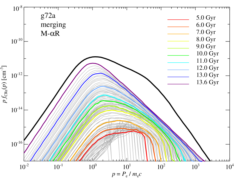
Figure 4: Differential spectral build up of the median electron distribution function, $f_{\mathrm{CRe}}$, as a function of cosmic time, for a post-merging cluster in the region between $(0.8-1.0)\,R_{200}$. The black solid line shows the total $f_{\mathrm{CRe}}$. The thin grey lines show the individual differential contributions to $f_{\mathrm{CRe}}$ from different times, where we highlight the contributions spaced by Gyr intervals with different colors. The spectral features are shaped by different cooling processes: non-relativistic Coulomb cooling for $p<1$, a broad feature indicating the transition from relativistic Coulomb cooling to the adiabatic regime for $1<p\lesssim 10^{2}$, and inverse Compton cooling at higher momenta.

3.2 Analytic Model for Fossil Electrons

We develop an analytic model for the fossil distribution function $f_{\mathrm{CRe}}(p)$ in the presence of multiple cooling processes. There are two clear limiting cases: an “impulsive injection” scenario where an initial population of relativistic particles cools passively, and a “steady injection” scenario where a steady state balance between injection and cooling is achieved. The “impulsive” scenario is appropriate when the timescale between shocks is greater than the cooling time. The finite time resolution of our post-processed simulations means that our simulation results are a linear superposition of such impulsive solutions. The “steady state” scenario is appropriate when the injection rate of relativistic particles is fairly constant, and $t_{\rm cool}(p)\ll t_{\rm H}$ (where $t_{\rm H}$ is the Hubble time) so that the population equilibrates on a short timescale.

Naively, since the CRs are injected at discrete shocks, one might expect the impulsive approximation to be most appropriate. In fact, the opposite is true. The timescale on which the shock injection process changes is the dynamical time, $t_{\rm inj}\sim t_{\rm dyn}\sim t_{\rm H}/\sqrt{\Delta}\sim 0.6\,\Delta_{300}^{-1/2}$ Gyr, where $t_{\rm H}=10$ Gyr, $\Delta_{300}=\Delta/300$ and $\Delta=\rho/\bar{\rho}$. On, the other hand, as we shall soon see, the main regime of interest where cooling significantly modifies the spectrum is the trans- and sub-relativistic regime of Coulomb cooling, where $t_{\rm cool}\sim 0.6\,p^{3}(n_{\mathrm{e}}/3\times 10^{-5}\,{\rm cm^{-3}})^{-1}$ Gyr for $p<1$. The fact that $t_{\rm cool}\lower 2.15277pt\hbox{$\;\buildrel<\over{\sim}\;$}t_{\rm inj}$ implies that the injection rate is roughly constant on the cooling timescale over which the population equilibrates. Moreover, the Coulomb cooling rate itself—which depends on the gas density—changes on the dynamical time $t_{\rm dyn}$. Figure 5 shows the Lagrangian evolution of the physical gas density that ends up in the virial region of a cluster. The presence of clumping implies a non-Gaussian density distribution that biases the mean of the distribution upwards in comparison to the median, the latter of which also shows a much smoother density evolution. In fact, the physical density does not even evolve significantly on timescales $t\gg t_{\rm dyn}$. Thus, on the short equilibration timescale $t_{\rm cool}$ for the sub and trans-relativistic regimes, the injection and cooling rates are roughly constant, and a steady state solution is valid. However, before constructing these solutions, it is worthwhile to examine the injection and cooling processes in more detail.

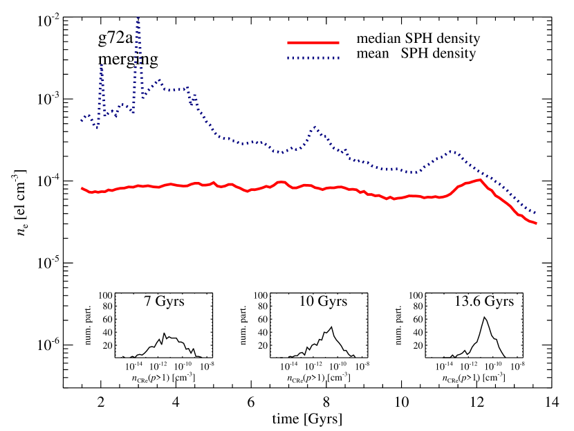
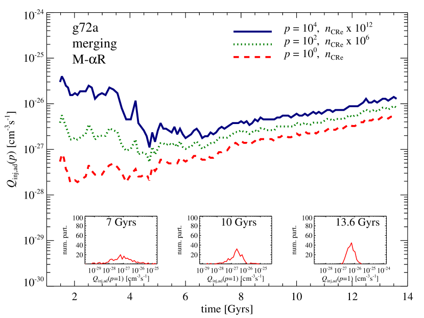
Figure 5: Lagrangian evolution of the thermal electron number density, $n_{\mathrm{e}}$ (left), and the injection rate density of CR electrons, $Q_{\rm inj,ad}$ (right). We consider a representative sample of SPH particles that end up at the virial region of a massive, post-merging cluster (g72a) between $(0.8-1.0)\,R_{200}$ at $z=0$ and follow their evolution as a function of time since the Big Bang. Left: the mean (blue dotted) and median (red solid) $n_{\mathrm{e}}$. Their difference is due to its non-Gaussian distribution caused by clumping, which biases the mean upwards. Right: we show $Q_{\rm inj,ad}$ for three different momenta: $p=1$ (red dashed ), $p=100$ (green dotted, weighted by factor $10^{6}$), and $p=10^{4}$ (blue solid, weighted by factor $10^{12}$). The three small insets in each panel show CR electrons with a momentum $p>1$ at different times; the density distribution of the fossil CR electrons (left), and the injection rate density (right). The variance is caused by different shock strengths, injection efficiencies, thermal densities and decreases with time.

The right-hand panel of Fig. 5 shows the Lagrangian evolution of the median CRe injection rate, $Q_{inj,ad}\sim\dot{n}_{CRe}$, of gas ending up in the outskirts of cluster g72a, which experienced a merger about 2 Gyrs ago. The merger is clearly visible in the density but not in the injection rate. This is because (1) only a fraction of the SPH particles that we trace in the simulations experience shocks induced by the merger, with a minor impact on the median injection rate, and (2) we account for the adiabatic cooling of the injected particles, which suppresses the injection rate for the merger with a factor $\sim C_{\mathrm{inj}}/C_{f}(\rho_{f}/\rho_{\mathrm{inj}})^{((a_{\mathrm{inj}}+2)/3)}\sim 4\times 4^{-4.5/3}\sim 0.5$. We can also see that the injection rate is fairly steady over cosmological timescales. Similarly, we have also found that the injection rate of a cool core cluster that has not experienced a major merger in the last 7 Gyrs is either decreasing slowly or constant with time. Note that this is only true for the median spectrum (or any other spectrum which is averaged over a large number of fluid elements). An individual fluid element can have a more stochastic injection history, and the fossil electron population in the outskirts of the cluster can vary spatially. This implies that when a weak shock propagates across a cluster, not all regions will light up with equal intensity. This spread in the CRe population is shown in the insets on the left panel of Fig. 5, while the spread in the injection rate is shown in the right panel. These distributions narrow with time, but can still span 1-2 dex at $z=0$.

For now, we focus on understanding the median spectrum. Figure 5 shows that the median density over the last $\sim$ Gyr is $n_{\mathrm{e}}\sim 3\times 10^{-5}\,{\rm cm^{-3}}$ (corresponding to $\Delta\sim 300$), while the median CRe injection rate density is $\dot{n}_{\rm CRe}(p>1)=\int_{1}^{\infty}Q_{\mathrm{inj,ad}}(p)\,\mathrm{d}p\sim Q_{\mathrm{inj,ad}}(p=1)\sim 4\times 10^{-27}{\rm cm^{-3}\,s^{-1}}$, where $Q_{\mathrm{inj,ad}}(p)=f_{\mathrm{inj,CRe}}(p,t)/\Delta t\,(\rho_{f}/\rho_{\mathrm{inj}})^{(\alpha+2)/3}$. We can understand this from simple order of magnitude arguments. From Fig. 3, the spectral index for the adiabatic spectrum is $\alpha\sim 2.5$, corresponding to $\mathcal{M}\sim 3$ shocks. This is consistent with Fig. 1 of Kang & Ryu (2011), where they find that the kinetic energy flux of shocks has a sharp drop-off for shocks with $\mathcal{M}\lower 2.15277pt\hbox{$\;\buildrel<\over{\sim}\;$}3$. A $\mathcal{M}\sim 3$ shock injects CRs at the cluster periphery with number density $n_{\mathrm{CRe}}(p>1)\sim n_{\mathrm{e}}\eta_{\rm CR,lin}(p_{*}/p_{\mathrm{inj}})^{-\alpha+1}\sim 3\times 10^{-11}\,{\rm cm^{-3}}$, where $\eta_{\rm CR,lin}=n_{\rm CR}/n_{\mathrm{e}}\sim 4\times 10^{-7}$ is the injection efficiency for a $\mathcal{M}=3$ shock (where $p_{\mathrm{inj}}\sim 4.4\,p_{\rm therm}$), and the factor of $(p_{*}/p_{\mathrm{inj}})^{-\alpha+1}$ converts $n(p>p_{\mathrm{inj}})$ to $n(p>p_{*})$, and $p_{*}\sim 1$. Since the shocks operate on a dynamical timescale $t_{\rm dyn}\sim t_{\rm H}/\sqrt{\Delta}\sim 0.6\,\mathrm{Gyr}\,\Delta_{300}^{-1/2}$, the estimated injection rate is $\dot{n}_{\rm CR}(p>1)\sim{n}_{\rm CRe}(p>1)/t_{\rm dyn}\sim 2\times 10^{-27}\,{\rm cm^{-3}\,s^{-1}}$, which agrees with the simulation results within a factor of two.

As for cooling, Fig. 1 illustrates the cooling time as a function of energy, for $n_{\mathrm{e}}\sim 10^{-5}{\rm cm^{-3}}$ at $z=0$. There is a quasi-adiabatic regime $p_{1}<p<p_{2}$ where $p_{1}\sim 10$, $p_{2}\sim 10^{2}$ where $t_{\rm cool}>t_{\rm H}$; otherwise, for $p<p_{1}$, Coulomb cooling dominates, while for $p>p_{2}$, inverse Compton cooling dominates. For our purposes, Coulomb cooling is the most important cooling process. Inverse Compton cooling merely shifts particles from the high energy tail to the adiabatic regime (which acts as a ’road-block’), where they are still available for reacceleration. Moreover, the relative number of affected particles in the power-law tail is relatively small. By contrast, Coulomb cooling affects the low-energy regime where most of the particles are by number, and can cause them to migrate to low thermal momenta, where they are no longer available for reacceleration. Note that the Coulomb cooling function (equation 24) undergoes a rapid transition from relativistic energies ($b_{\rm C}\approx{\rm const}$) to sub-relativistic energies ($b_{\rm C}\propto p^{-2}$), which implies cooling times $t_{\rm cool}\propto p$ (for $1\lesssim p\lesssim 30$, where the upper limit depends on density and redshift) and $t_{\rm cool}\propto p^{3}$ (for $p<1$). This rapid thermalization of sub-relativistic particles creates a peak in the steady state spectrum at $p\sim 1$.

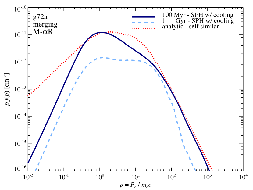
Figure 6: Comparison of the self-similar model (red dotted) of equation (28) to the median CRe spectra, $f_{\mathrm{CRe}}$, of our simulated post-merging cluster g72a. We show the median $f_{\mathrm{CRe}}$ for two different time resolutions, 100 Myr (dark blue solid) and 1 Gyr (light blue dashed), indicating impressive convergence at $p\gtrsim 100$, which is the relevant energy regime for radio relic emission.

Let us now consider a toy model where the injection and Coulomb cooling rates are constant. As previously mentioned, this is a reasonable approximation, as they both change on a dynamical time $t_{\rm dyn}$ which is longer than the equilibration time $t_{\rm cool}$. For the same reason, we can ignore adiabatic changes to the electron spectrum. The magnetic fields which govern synchrotron cooling also change on a dynamical time (for adiabatic changes, or a turbulent dynamo), while inverse Compton cooling changes on cosmological timescales. It is straightforward to solve for the steady state solution, using the Vlasov equation. However, this is only appropriate in the low and high energy regimes, where cooling (and hence equilibration) timescales are short. In the adiabatic regime ($p_{1}<p<p_{2}$), the electron population is time-dependent—it simply grows with time. Fortunately, when the injection and cooling function are time-independent, one can construct self-similar solutions which connect the steady and non-steady populations (Sarazin, 1999). In these solutions, the overall normalization varies with time, but the shape of the energy spectrum remains the same if $p$ is scaled by some characteristic value. It is:

$$f_{\rm self-sim}(p,t) \approx \frac{Q_{\rm inj,ad}(p)\,\Delta t}{{a_{\mathrm{inj}}-1}}\,\left(\frac{\tilde{p}_{\mathrm{Coul}}}{p}+\frac{p}{\tilde{p}_{\mathrm{IC}}}\right)^{-1}$$ (28)

$$\times \left\{2-\left[\frac{1}{2}\left(1-\frac{p}{\tilde{p}_{\mathrm{IC}}}+\left|1-\frac{p}{\tilde{p}_{\mathrm{IC}}}\right|\right)\right]^{a_{\mathrm{inj}}-1}\right.$$

$$- \left.\left(1+\frac{\tilde{p}_{\mathrm{Coul}}}{p}\right)^{-(a_{\mathrm{inj}}-1)}\right\}\,.$$

The approximation in equation (28) is valid as long as $\tilde{p}_{\mathrm{IC}}\gg\tilde{p}_{\mathrm{Coul}}$, where $\tilde{p}_{\mathrm{IC}}\sim 1/(b_{\mathrm{IC,0}}\,\Delta t)$, and $\tilde{p}_{\mathrm{Coul}}\sim b_{\mathrm{C}}(p,t)\,\Delta t$ . This expression explicitly makes the approximation that the injection rate $Q_{\rm inj,ad}$ and cooling rates $b_{\rm C},b_{\rm IC}$ are independent of time. It thus only requires two time-independent input parameters, $Q_{\rm inj,ad},n_{\rm e}$. In Appendix C we provide a power-law model for $Q_{\rm inj,ad}$ with the spectral index $a_{\mathrm{inj}}$. In Fig. 6, we compare the results of our simulations of g72a (which have 100 Myr time resolution) to the self-similar model in equation (28). The agreement is remarkable, given that injection and cooling rates are not exactly constant. We also show a calculation with lower time-resolution $\Delta t=1$ Gyr, where the agreement is worse, especially in the momentum regime where IC cooling is substantial. The reason for this is that there are less SPH particles, which got recently injected. Hence IC cooling modified the spectrum more severely and removed all CRes with a momentum above $p_{\mathrm{IC}}$. As a result, median spectrum is biased low at high energies. We shall return to this issue of finite time resolution in §4.2.

4 Reacceleration

4.1 Which Momentum Regime Matters?

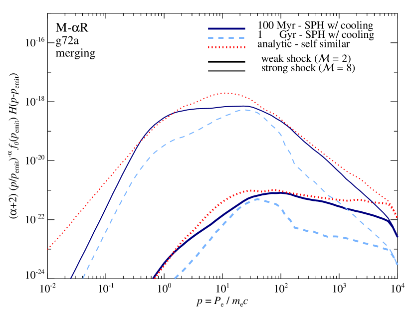
Figure 7: We show the contribution per logarithmic interval in momentum to the integral of the downstream distribution function of reaccelerated CR electrons in equation (30). For a strong shock ($\mathcal{M}\gtrsim 4$), there is a broad peak of fossil electrons with $1\lesssim p\lesssim 100$ dominate the contribution to reaccelerated CR electron distribution, while for a weak shock, higher momenta with $p\gtrsim 10$ contribute equally.

Downstream of a shock, the CR distribution function can be written as (Bell, 1978b; Drury, 1983b):

$$f_{2}(p) = (\alpha+2)\,p^{-\alpha}\,\int_{p_{\rm inj}}^{p}p^{\prime\alpha-1}f_{0}(p^{\prime})\,\mathrm{d}p^{\prime}$$ (29)

$$+ f_{\rm inj}\left(\frac{p}{p_{\rm inj}}\right)^{-\alpha}H(p-p_{\rm inj})\,,$$

where $\alpha$ is the test particle power-law slope and $H(p-p_{\rm inj})$ is the Heaviside step function, and $f_{0}(p^{\prime})$ represents the fossil CR electron population upstream of the merger shock, mimicking the conditions for a radio relic. The first and second terms on the right hand side refer to the contribution of relic and freshly injected CRs respectively; we focus on understanding the former in this section. This first term can be written in a more physically instructive way as (Drury, 1983b):

$$f_{2}^{\rm reaccel}(p)=\int_{p_{\rm inj}}^{\infty}(\alpha+2)\left(\frac{p}{p^{\prime}}\right)^{-\alpha}f_{0}(p^{\prime})H(p-p^{\prime})\mathrm{d}({\rm log}p^{\prime})\,.$$ (30)

Thus, the downstream spectrum is a convolution of the upstream spectrum with a truncated power-law. Note that since particles are conserved and do not lose energy during the acceleration process, we expect $n_{2}^{\rm reaccel}(p>p_{\rm inj})=rn_{0}^{\rm fossil}(p>p_{\rm inj})$, where $r=\rho_{2}/\rho_{0}$ is the shock compression ratio. Indeed one can derive equation (30) from this assumption. These statements are reminiscent of the manner in which a thermal Maxwellian tail with $p>p_{\rm inj}$ is converted into a power-law—nothing about the acceleration process relies upon a Maxwellian distribution, and the same conclusions hold for a non-Maxwellian tail.

For concreteness, an illustrative example can be useful. Consider the case when the relic spectrum is a power-law $f_{0}(p)=f_{0,*}(p/p_{\rm*})^{-\beta}H(p-p_{*})$ (Kang & Ryu, 2011; Kang et al., 2012). Substituting $f_{0}(p)$ into equation (30) yields for $\alpha\neq\beta$ (Kang & Ryu, 2011):

$$f_{2}(p) = \frac{\alpha+2}{(\alpha-\beta)}\left[1-\left(\frac{p}{p_{\rm*}}\right)^{-\alpha+\beta}\right]f_{0}(p)$$ (31)

$$\approx \frac{\alpha+2}{|\alpha-\beta|}f_{0,*}\left(\frac{p}{p_{\rm*}}\right)^{-\gamma},\ \ \ p\gg p_{\rm*}\,,$$ (32)

where $\gamma={\rm min}(\alpha,\beta)$. Thus, for $p\gg p^{*}$, the reaccelerated distribution function asymptotically becomes a power-law, with a spectral slope corresponding to the shallower (i.e., harder) of the initial spectrum and the reaccelerating shock. Of course, our fossil electron spectrum is very different from a power-law, due the effects of cooling: it is a sharply peaked function, with a continuously varying slope. Given that our simulations are only accurate in a limited momentum range $p^{\prime}$, we can ask: what range of $p^{\prime}$ must crucially be resolved? Naively, one might assume that that since reacceleration conserves number density, it suffices to resolve the peak of $p^{\prime}f(p^{\prime})$, where most particles reside. However, the additional weighting by a power-law in equation (30) means that this condition is insufficient: although $p^{\prime}f(p^{\prime})$ robustly peaks at $p^{\prime}\sim 1$, electrons here may be ’too far from the action’, once multiplied by the lever arm $(p_{\rm emit}/p^{\prime})^{-\alpha}$.

Let us consider which initial momentum regime contributes most to observed synchrotron emission of reaccelerated fossils. The characteristic synchrotron frequency is $\sim 3\gamma^{2}\nu_{\mathrm{c}}$, where $\nu_{\mathrm{c}}$ is the non-relativistic cyclotron frequency; this implies that for a given observation frequency $\nu_{\mathrm{s}}$, the greatest contribution comes from electrons with

$$p_{\rm emit}\approx\gamma_{\rm emit}\approx 5\times 10^{3}\left(\frac{\nu_{\mathrm{s}}}{1\,{\rm GHz}}\right)^{1/2}\left(\frac{B}{5\,\mu{\rm G}}\right)^{-1/2}(1+z)^{1/2},$$ (33)

where for instance $B\approx 5\,\mu$G has been inferred from high resolution measurements of spectral aging in the sausage relic (van Weeren et al., 2010). Figure 7 illustrates the contribution per logarithmic interval to the integral in equation (30), for $p_{\rm emit}=10^{4}$. For a strong shock, we see that the integrand has a broad peak ranging from $1\lower 2.15277pt\hbox{$\;\buildrel<\over{\sim}\;$}p^{\prime}\lower 2.15277pt\hbox{$\;\buildrel<\over{\sim}\;$}100$, while for a weak shock it increases monotonically with $p^{\prime}$, receiving its dominant contribution from $10^{2}\lower 2.15277pt\hbox{$\;\buildrel<\over{\sim}\;$}p^{\prime}\lower 2.15277pt\hbox{$\;\buildrel<\over{\sim}\;$}10^{4}$.

We can understand this as follows. The integrand peaks when $\alpha-\beta(p^{\prime})=0$, where $\beta(p^{\prime})=-d\log\,f_{0}/d\log\,p^{\prime}$, i.e. when the power-law slope of reaccelerated particles and the fossil distribution function have the same slope. It picks up most of its contributions from a neighborhood of this region. From Fig. 3, we see that $\beta(p^{\prime})$ ranges from zero (due to NR Coulomb cooling) to extremely steep positive slopes $\beta(p^{\prime})>3$ (due to inverse Compton and synchrotron cooling), this tangent is guaranteed to exist. In practice, the relevant regime where $2<\beta(p^{\prime})<3$ lies in $1\lower 2.15277pt\hbox{$\;\buildrel<\over{\sim}\;$}p^{\prime}\lower 2.15277pt\hbox{$\;\buildrel<\over{\sim}\;$}10^{3}$, the ’adiabatic’ regime which only only mildly affected by relativistic Coulomb cooling or inverse Compton cooling. Regions which have much shorter cooling times and consequently had their injected slopes strongly modified do not contribute significantly. This suggests the fortunate conclusion that we do not need to accurately resolve regions strongly affected by cooling to accurately predict the reaccelerated spectrum. An important point to note is that in this crucial adiabatic momentum regime $1\lower 2.15277pt\hbox{$\;\buildrel<\over{\sim}\;$}p\lower 2.15277pt\hbox{$\;\buildrel<\over{\sim}\;$}100$, the spectral index of the injected spectrum $\alpha\approx 2.5$ (e.g., see bottom panel of Fig. 3), indicating that weak shocks ($\mathcal{M}\sim 3$) dominate the assembly of the fossil CRe spectrum here. We will return to this point in §5.1.

4.2 Do Our Simulations Have Sufficient Time Resolution?

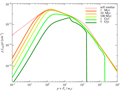
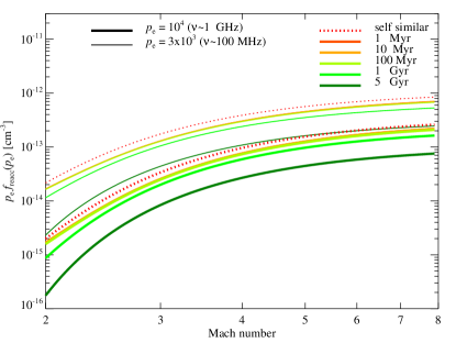
Figure 8: Continuous versus discrete injection. We show the cooled fossil CR electron distribution function as a function of normalized momentum. The self similar distribution (red dotted) assumes constant continuous injection and constant density and is compared to discrete injection scenarios of CRes with different duty cycles: 1 Myr (dark orange), 10 Myr (light orange), 100 Myr (light green), 1 Gyr (green), 5 Gyr (dark green). We assume an injected CR electron population given by equation (57) and an electron number density, $n_{\mathrm{e}}=3\times 10^{-5}\,\mathrm{cm}^{-3}$. The distribution function from discrete injection approaches the self similar solution when the injection timescale becomes smaller than the cooling time. Note that for this figure we adopt a characteristic assembly time of the CRes of 10 Gyrs, hence the 5 Gyrs curve (at $p=10$) and the 1 Gyr curve (at $p=10^{3}$) are superpositions of two and ten injected spectra, respectively, which explains the visible shoulders for these curves.

We now turn directly to the question of required time resolution. Our finding in §3.2 that injection and cooling is roughly time steady appears to contradict the approach we have taken in our simulations, where we inject CRes in discrete bursts (due to finite time resolution). In Fig. 8, we show the distribution function obtained by mimicking the same procedure we followed in our simulations: injecting the electrons in discrete bursts, and then passively cooling the injected population from each time step, via equations (53)-(55), for different values of $\Delta t$ (in our simulations, $\Delta t=(100\,\mathrm{Myrs}-1.5\,\mathrm{Gyrs})$, see Table 1 for details). For a fair comparison, we have assumed that cooling and injection are exactly constant. By comparison with the left panel in Fig. 8, we see that in regions where $\Delta t<t_{\rm cool}$, our computational procedure correctly approaches the analytic solution. However, when $\Delta t>t_{\rm cool}$, the discrete grid overestimates the importance of cooling, causing the numerical solution to fall below the analytic one.

However, our results from the previous section suggest that the regions where cooling is important do not contribute significantly to $f(p_{\rm emit})$. In particular, the main important mechanism is non-relativistic Coulomb cooling at $p\lower 2.15277pt\hbox{$\;\buildrel<\over{\sim}\;$}1$. This momentum regime of the fossil spectrum does not contribute significantly to $f(p_{\rm emit})$ (as in Fig. 7) because it is ’too far from the action’ at $p_{\rm emit}$, and also has been significantly depopulated. Thus, our finite time resolution does not significantly affect results. We show this explicitly in the right panel in Fig. 8, which shows $p_{\rm emit}\,f_{\rm reacc}(p_{\rm emit})$ from the reaccelerated population for the various curves in the left panel of Fig. 8, as a function of shock Mach number. The differences are small, given other uncertainties in the problem. This shows that the contribution from fossil reacceleration can indeed be estimated accurately analytically. Simulations are nonetheless invaluable for their ability to shed light on spatial (see the insets of Fig. 5) and temporal variations (see §5.2) in injection and cooling rates, all of which can lead to significant scatter in the CRe fossil population.

4.3 Principal Result: Reacceleration Dominates over Direct Injection

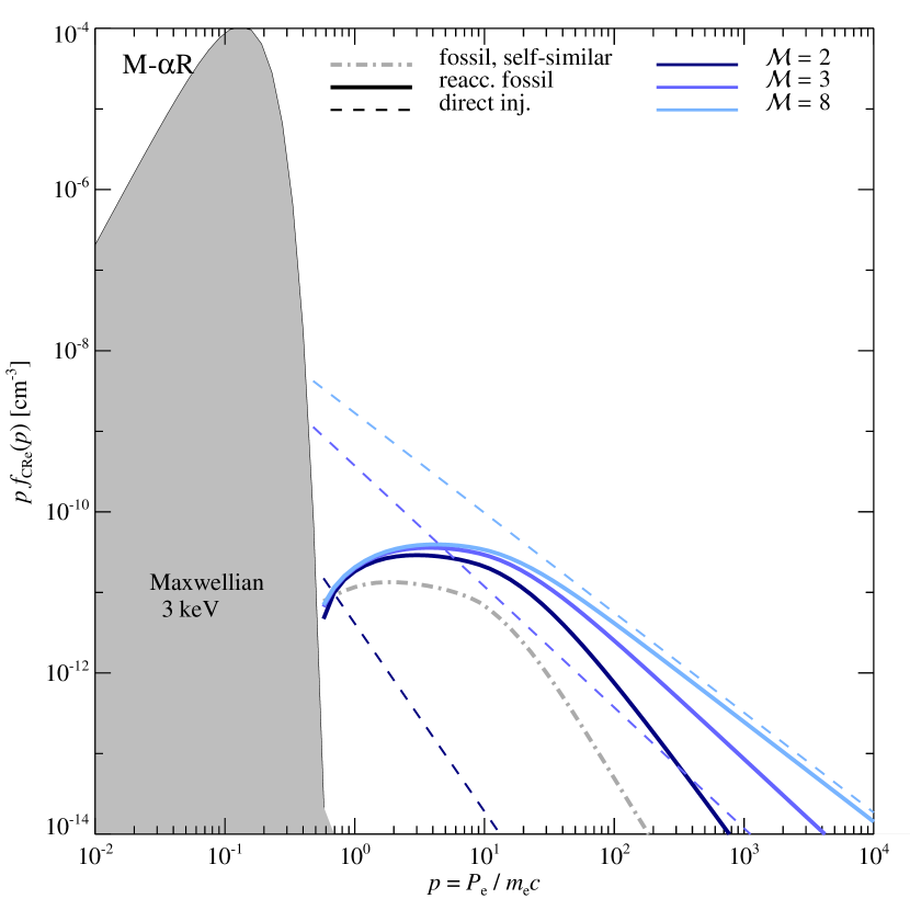
Figure 9: Median $pf_{\rm CRe}$ for direct injection (dashed line) and reacceleration (solid line), for different Mach numbers (color coded); also shown is the fossil distribution function (dot-dashed). $f_{\rm CRe}$ for direct injection is a power-law attached to the Maxwellian, while the reaccelerated $f_{\mathrm{CRe}}$ is a boosted version of the fossil distribution function, with an asymptotic power-law tail. The distribution function falls much more drastically at low Mach number for direct injection (dashed) than for reacceleration (solid).

Thus far, we have focused on accurate calculations of the fossil electron distribution function. We now explicitly illustrate, using equation (30), how this population of electrons is transformed and boosted by a shock. Figure 9 shows the initial fossil electron distribution function and the transformed distribution function after Mach number ${\mathcal{M}}=2,3,8$ shocks; the population due to direct injection is also shown. The distribution function for direct injection is a power-law attached to the Maxwellian, while the reaccelerated distribution function is a boosted version of the fossil distribution function, with an asymptotic power-law tail. This tail has the same power-law slope $\alpha$ as for direct injection. Note that while the total number of fossil electrons is conserved, the number density of reaccelerated electrons increases over that of the fossil population by the shock compression factor $r$, which explains the normalization boost upon reacceleration. It is clear that while the electrons from direct injection have a strong Mach number dependence, this trend is much weaker for the reaccelerated population. This suggests that reacceleration could dominate at low Mach numbers.

Figure 10 shows the main result of this paper, the ratio $f_{\rm reacc}(p_{\rm emit})/f_{\rm inj}(p_{\rm emit})$, or the ratio of the distribution function at the primary emitting frequency for the reaccelerated population to the same for the freshly injected population (dark blue curve). We see that at high Mach numbers (${\mathcal{M}}>4$), relic reacceleration and fresh injection are comparable, but for low Mach numbers (${\mathcal{M}}<4$), fossil reacceleration vastly dominates over fresh injection. We also compare the reacceleration and direct injection models to a straw man model (‘M-const’) where a constant fraction of the shock energy $\zeta_{\rm inj,e}=0.01$ is converted to relativistic electrons, independent of Mach number. As previously mentioned, while we do not believe this assumption to be physically realistic, it has been widely used in the literature, and gives us a baseline for comparison. While the ‘M-const’ model gives comparable results to the other two models for ${\mathcal{M}}>4$, it differs sharply from the direct injection model for ${\mathcal{M}}<4$, over-predicting the CRe population. This makes sense, since physically we expect the injection efficiency to plummet at low Mach numbers. By contrast, the ‘M-const’ model is similar to the reacceleration model down to ${\mathcal{M}}\sim 3$, but for ${\mathcal{M}}<3$ it under-predicts the CRe population. This has two important consequences. Firstly, it means that ‘M-const’ models have been getting the right answer for the wrong reasons: while they can match observations of ${\mathcal{M}}\lower 2.15277pt\hbox{$\;\buildrel>\over{\sim}\;$}3$ relics, this is not necessarily because acceleration efficiency is independent of Mach number. Instead, our model provides a physical basis for the observed brightness of low Mach number relics, through the existence of fossil CRe (see also Fig. 16). Secondly, at extremely low Mach numbers ${\mathcal{M}}<3$, reacceleration predicts many more CRe than even this model. Thus, we predict many more relics with steep spectra which are potentially observable with LOFAR (see § 6).

How can we understand the Mach number dependence of $f_{\rm reacc}(p_{\rm emit})/f_{\rm inj}(p_{\rm emit})$? It is easy to understand why it rises steeply at low Mach numbers. The Mach number dependence of $f_{\rm reacc}(p_{\rm emit})$ is solely due to the dependence of the power-law slope $\alpha$ on Mach number; the number of particles available for acceleration is fixed. As $\alpha$ steepens at low Mach number, $f_{\rm reacc}(p_{\rm emit})$ falls in a power-law fashion. This mostly happens for ${\mathcal{M}}\lower 2.15277pt\hbox{$\;\buildrel<\over{\sim}\;$}4$, when $\alpha$ begins to evolve significantly. On the other hand, fresh injection is affected both by the change in $\alpha$ and more importantly, the change in the number of particles available for acceleration. As can be easily derived from the jump conditions, low Mach number shocks have lower thermalization efficiencies: the post-shock gas has a lower temperature and higher bulk velocity. This means that $x_{\rm inj}=p_{\rm inj}/p_{\rm therm}$ has to be higher for a particle to be able to overcome the bulk fluid motion to cross the shock. This increase in $x_{\rm inj}$ on the Maxwellian tail exponentially reduces the number of particles which are accelerated at low Mach number shocks, which is why $f_{\rm inj}(p_{\rm emit})$ is exponentially suppressed.

On the other hand, the fact that $f_{\rm reacc}(p_{\rm emit})$ and $f_{\rm inj}(p_{\rm emit})$ are roughly comparable at high Mach numbers may appear somewhat surprising. Since the build-up of the CRe fossil population is due to the interaction of continuous injection via multiple shocks with cooling processes, a priori we might expect that it could potentially be orders of magnitude smaller or larger than that due to direct injection at a single shock. In particular, as we have seen in Fig. 7, since much of the contribution to $f_{\rm reacc}(p_{\rm emit})$ comes from an adiabatic regime which grows monotonically on cosmological timescales, we might expect the reservoir of fossil CRe built up to outweigh the contribution from a single shock. In fact, as seen in Fig. 4 and Fig. 5, the injection rate is fairly time-steady, with late times having a somewhat larger contribution since the gas is getting hotter, increasing $p_{\rm therm}$. The characteristic injection timescale is $t_{\rm dyn}\sim t_{\rm H}/\sqrt{\Delta}\sim 1$ Gyr, implying that the fossil CR electron population should be $t_{\rm H}/t_{\rm dyn}\sim 10$ times larger. The fact that cooling operates, and the reduced contribution from early times makes the value of $f_{\rm reacc}(p_{\rm emit})/f_{\rm inj}(p_{\rm emit})\sim 1$ shown in Fig. 10 reasonable. We also note that the fossil CRe population can show significant scatter from cluster to cluster, up to an order of magnitude (which we shall discuss in §5.2), so one should not over-interpret the exact value of $f_{\rm reacc}(p_{\rm emit})/f_{\rm inj}(p_{\rm emit})$.

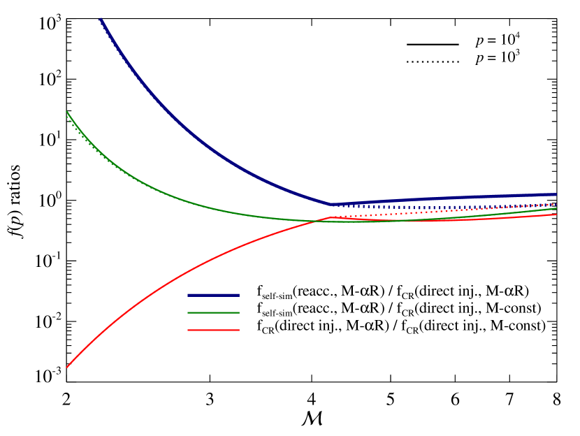
Figure 10: The ratio of the distribution function evaluated at $p\equiv P_{\mathrm{e}}/m_{\mathrm{e}}\,c=10^{3}$ (dotted) and $10^{4}$ (solid), for different acceleration models. The fiducial dark blue curves show $f_{\rm CR}({\rm reacc.})/f_{\rm CR}({\rm inj})$. Reacceleration is roughly comparable to direct injection at high Mach numbers and vastly exceeds direct injection at low Mach numbers. The green (red) curves compare reacceleration (direct injection) with a strawman model–commonly used in the literature–where a constant fraction $\zeta_{\rm inj,e}=0.01$ of the shock energy goes into electrons, independent of Mach number. The straw man model has roughly similar behavior to the other models at high Mach number, but vastly divergent behavior at low Mach number. Note that the reaccelerated CRe fossil population, $f_{\rm CR}({\rm reacc.})$, is derived from the self-similar model in equation (28) using a characteristic cooling time $\Delta t\sim 9$ Gyrs.

5 Variations in the Fossil Electron Spectrum

5.1 Dependence on Shock Acceleration Model

In §2.2.3, we discussed 3 different models for particle acceleration, but thus far largely used one model (‘M-$\alpha$R’) to compute the fossil electron spectrum. Fig. 10 has already highlighted differences between the ‘M-$\alpha$R’ model and the ‘M-const’ model for a single shock. We now propagate these differences between the three models when the entire assembly history of the fossil population is taken into account.

The resulting fossil electron population for the test particle model (‘M-testp’), the CRe spectral index renormalization model (‘M-$\alpha$R’), and the model with constant acceleration efficiency $\zeta_{\rm inj,e}=1$ per cent (‘M-const’) is shown in Fig. 11. We see that while the ‘M-$\alpha$R’ and ’M-testp’ models give very similar results, the ‘M-const’ model yields a fossil distribution function with a significantly higher normalization.

These results are easy to understand. From the bottom panel of Fig. 3 (and discussed in §4.1), we see that the spectral index of the median injected population before cooling is $\alpha_{e}\sim 2.5$, i.e., weak shocks with ${\mathcal{M}}\sim 3$ dominate the assembly of the CRe fossil population. The ‘M-$\alpha$R and ‘M-testp’ models are identical at low Mach numbers; they only differ in how energy conservation is enforced at high Mach numbers (even so, differences are slight). By contrast, the ‘M-const’ model is broadly similar to the other models at high Mach numbers, but diverges sharply at low Mach numbers, with a significantly higher normalization (c.f. the red curve in Fig. 10), since by construction $\zeta_{\rm e,inj}$ is constant, whereas it plummets drastically at low ${\mathcal{M}}$ for the other models. Since fossil CRes are primarily put in place by weak shocks, it is not surprising that they are much more abundant in this model. This amounts then to an increase in normalization of the ‘M-const’ model by roughly an order of magnitude in comparison to the other models (as can be inferred for the acceleration efficiency at $\mathcal{M}=3$ shocks from Figs. 10 and 2, considering that the relevant shocks are preferentially those at late time in a hot medium with particle energies of a few keV).

These results indicate our main conclusion that fossil reacceleration must dominate at low Mach number is independent of the shock acceleration model. If one attempts to explain the observed brightness of weak shocks by modifying shock physics and increasing the acceleration efficiencies at low ${\mathcal{M}}$, the same would hold for previous weak shocks and the normalization of the fossil CRe population would be correspondingly larger. Since the shock acceleration efficiency largely cancels out, the relative importance of reacceleration vs. direct injection depends on accretion/merger history and cooling, for which (unlike shock acceleration) there is relatively little uncertainty in the physics.

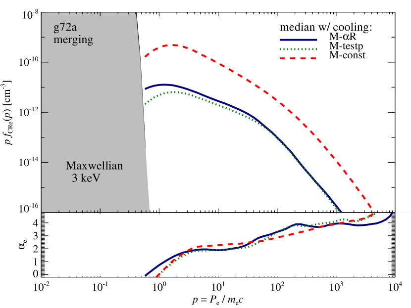
Figure 11: Comparison of median CRe spectra in the cluster outskirts of g72a at $z=0$ in different acceleration models. Shown are the test particle model (‘M-testp’), the CRe spectral index renormalization model (‘M-$\alpha$R’), and the model with constant acceleration efficiency $\zeta_{\rm inj,e}=0.01$ (‘M-const’).

5.2 Cluster-to-Cluster variations

Is the build-up of a CRe spectrum in cluster outskirts a universal process? To answer this question, we compare the CRe distribution for three typical clusters at different times in Fig. 12: a small cool core cluster, a large cool core cluster, and a large post-merger cluster. It is remarkable how similar the spectral shape is between the different clusters and at different times. This generic shape can be understood from the analytic model presented in §3.2. The peak is at $p\sim 1$ and the normalization for each cluster changes by a factor less than 10. The recent merger cluster g72a shows the highest CRe number density, while the CRes in the two cool core clusters have a lower abundance.

What is the origin of this dispersion? Does it originate from differences in CRe injection or cooling, between clusters? In Fig. 13, we show the CRe spectra for all 14 clusters, both with (blue) and without (green) cooling. The adiabatic spectra (which were only transported adiabatically without accounting for cooling) exhibit remarkably little scatter, while the cooled spectra show considerably more scatter. This suggests that the variance between clusters arises from the cooling rather than the injection process (for more on scatter in the adiabatic spectrum, see Appendix C and Fig. 20).

Two other features in Fig. 13 are worth noting. Firstly, cooling introduces increased scatter even in the ostensibly quasi-adiabatic regime $10\lower 2.15277pt\hbox{$\;\buildrel<\over{\sim}\;$}p\lower 2.15277pt\hbox{$\;\buildrel<\over{\sim}\;$}100$. Note that this regime has $t_{\rm cool}>t_{\rm H}$ only for $n_{e}\lower 2.15277pt\hbox{$\;\buildrel<\over{\sim}\;$}10^{-5}\,{\rm cm^{-3}}$ and at $z=0$. For higher gas densities and redshifts, some cooling is possible; thus, variations in gas clumping (which affects the amount of Coulomb cooling) and shock history (which affects the total amount of cooling; cf. the difference between “impulsive” and “continuous injection” solutions). The fact that there is substantial scatter at $p\sim 100$ (where only inverse Compton cooling is important) points toward the latter. Namely, clusters which receive their dose of CRes earlier than others undergo more inverse Compton cooling. The different build-up and normalization of the CRe population in the cool core and recent merger clusters in Fig. 12 also supports this. Secondly, the scatter at low $p$ is considerably higher than at high $p$. Part of this is because the cooling time is shorter at low $p$, and hence differences in shock history–which are averaged over shorter timescales–are amplified. However, part of the difference is artificial, and due to our finite time resolution, which overestimates the effects of cooling (§4.2 and Fig. 8). For instance, the two clusters with the higher normalizations in the Coulomb cooling regime are g72a and g72b, which have a time resolution ten times better than the other clusters. Fortunately, as shown in §4.1, this momentum regime is unimportant in its contribution to the reaccelerated spectrum at $p_{\rm emit}$. By contrast, the cooling time is generally longer than our time resolution in the $p\lower 2.15277pt\hbox{$\;\buildrel>\over{\sim}\;$}10$ regime.

Finally, by integrating over momentum (equation 30), we show the scatter in the observationally more relevant quantity $p_{\rm emit}f(p_{\rm emit})$, where $p_{\rm emit}\sim 10^{4}$, in Fig. 14, plotted against cluster mass $M_{200}$. The scatter is about an order of magnitude, and somewhat below the apparent scatter in Fig. 13, since it is weighted towards the lower scatter, high $p$ regime. There may be a trend for the CRe distribution function to increase with $M_{200}$ for merging clusters, though our sample size is too small to make definitive statements.

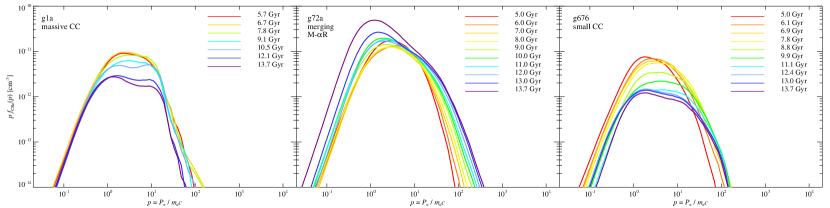
Figure 12: Lagrangian evolution of CRe spectra of three different clusters. We show the median CRe distribution function of a representative sample of SPH particles that all end up at $z=0$ in the virial regions within $(0.8-1.0)\,R_{200}$ (different time intervals since Big Bang are color coded). Shown are a large cool core cluster (g1a, left), a cluster with a recent merger (g72a, middle), and a small cool core cluster (g676, right). There is strong evolution of $f_{\mathrm{CRe}}$ in the post-merger cluster, which is noticeably reduced in the cool core clusters. While the normalization is increasing in our post-merger cluster that experienced a more violent recent history, the opposite trend is visible in the cool core clusters where CRe cooling processes dominate. However, the overall shape of the distribution function is very similar between those clusters that vary widely in dynamical stage and mass.

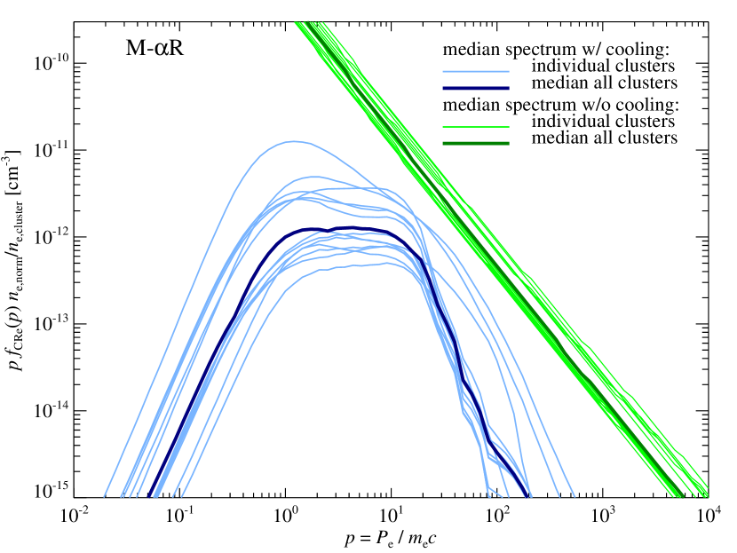
Figure 13: CRe spectra in the virial regions of clusters at $z=0$. Shown are the median CRe spectra of all simulated clusters normalized to the same thermal electron number density $n_{\mathrm{e,norm}}=3\times 10^{-5}\,\mathrm{cm}^{-3}$; with cooling (light blue) and the median of those (dark blue), injected spectra (light green) and the median of those (dark green). The injected spectrum appears quite universal with little scatter. By contrast, although the cooled spectra all have similar shapes, their normalizations can differ substantially, by up to a factor of $\sim 50$.

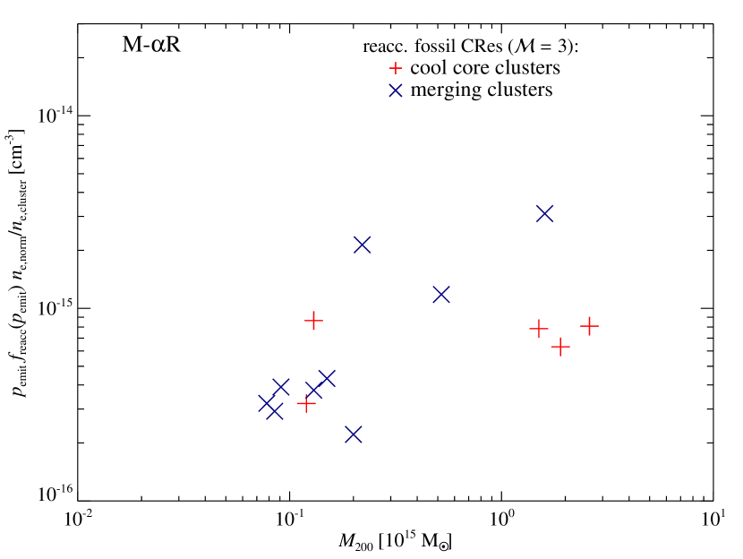
Figure 14: The momentum integrated quantity $p_{\rm emit}f(p_{\rm emit})$ (where $p_{\rm emit}\sim 10^{4}$) plotted against cluster mass. For each cluster the CRes are normalized to the same thermal electron number density $n_{\mathrm{e,norm}}=3\times 10^{-5}\,\mathrm{cm}^{-3}$. The red crosses and blue $X$ show the simulated cool core (CC) and merging clusters, respectively.

5.3 Radial variations of the fossil electron spectrum

To quantify the potential bias from the uncertainty in the distance of relics to the cluster center, we explore in Fig. 15 the radial variations of both the fossil CRe spectrum and CRes that are reaccelerated in typical merger shocks. To this end, we probe three radial bins; $(0.5-0.7)\,R_{200}\sim R_{500}$, $(0.8-1.0)\,R_{200}$ (the main focus of this paper), and $(1.1-1.3)\,R_{200}\sim R_{\mathrm{vir}}$. We find that the distribution of fossil CRes in the non-relativistic Coulomb cooling regime and high energy IC regime is sensitive to the radius. The variation at low momenta (due to the difference in Coulomb cooling; the density increases inward by a factor of 2-3 in each radial bin) is larger; variations at high momenta (due to differences in IC cooling, which is density independent and only varies with the relative injection history) are smaller. In contrast, at intermediate momenta, $p\sim 1-10$, there are almost no differences between the median distribution functions of our cluster sample. We have already seen such flat radial variations in CRp profiles (Pinzke & Pfrommer, 2010) (note that CRp’s are effectively adiabatic due to inefficient cooling). Indeed, in the hadronic model, a flat inferred CRp profile is required to explain the surface brightness profile in giant radio halos such as Coma (Zandanel et al., 2012). The fact that the CR number density is flat with radius implies that the relative number density of CRs $\eta=n_{\rm CRe}(>p^{\prime})/n_{\rm th}$ increases with radius. This may seems surprising, given that the cluster outskirts are generally assembled via weaker shocks, due to the slowdown of structure formation in a $\Lambda$CDM universe. As discussed in §3.1, this effect arises because the distribution function from later shocks have higher normalization: they take place in a hotter medium, so that $p_{\rm inj}\propto T^{1/2}$ attaches to the thermal distribution at higher momenta. This effect is apparently sufficiently to render $n_{\rm CRe}(>p^{\prime})\sim$ const.

The spectral shape of the fossil CRe distribution functions is similar between clusters, however, the normalizations can differ up to a factor 100. The spectral shape is also similar between different radial bins, indicating similar injection and cooling histories. In the right panel of Fig. 15 we explore the reaccelerated fossil population at $p=10^{4}$ for different Mach numbers of merger shocks. We find an increasing abundance of reaccelerated CRes for smaller radii. The reason is that the reaccelerated CRe populations for $\mathcal{M}>2$ shocks, are mainly build up from the CRes with $p>10$, hence we expect a factor $1-3$ difference between the different radii.

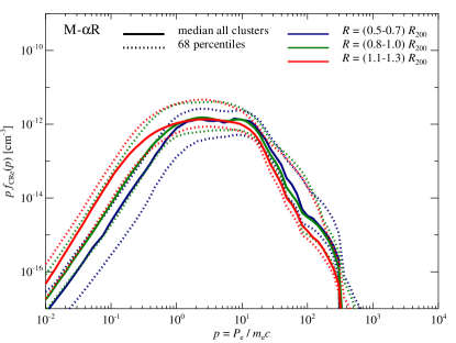
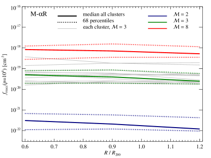
Figure 15: Radial variations of the fossil CRe spectrum in different clusters. We show the CRe distribution function, where the solid lines represent the median of all clusters, the dotted lines the 68 percentiles. In the left panel we show the fossil distribution function as a function of momentum where the colors represent different radial bins: blue line $(0.5-0.7)\,R_{200}$, green line $(0.8-1.0)\,R_{200}$, and red line $(1.1-1.3)\,R_{200}$. In the right panel we show the reaccelerated distribution function at momentum $p=10^{4}$ as a function of radius where the colors represent different Mach numbers of the reaccelerating shock: $\mathcal{M}=2$ (blue), $\mathcal{M}=3$ (green), and $\mathcal{M}=8$ (red). The thin grey lines show the reaccelerated CRe spectra for a $\mathcal{M}=3$ shock in each individual cluster. The reaccelerated spectra at $p=10^{4}$ show only a very weak radial trend.

6 Comparison with Radio Relic Observations

Table 2: Relic sample. For simplicity we assume a downstream magnetic field of 5 $\mathrm{\mu G}$ and a downstream temperature of $kT_{2}=5$ keV.

relic name	redshift	$\mathcal{M}^{(1)}$	$\Psi_{\mathrm{S}}^{(2)}$	thickness(3)	$n_{\mathrm{e}}^{(4)}$	$P$(1.4 GHz)	reference
			[Mpc2]	[kpc]	[el cm-3]	[$10^{32}$ erg s-1 Hz-1]
A 2256	0.0594	2.6	0.6	70	$\,\,10^{-3}$	0.4	Clarke et al. (2011)
A 3667	0.055	4.7	2.0	62	$8\times 10^{-5}$	4.1	Röttgering et al. (1997)
Sausage	0.1921	4.5	1.5	48	$3\times 10^{-5}$	1.4	van Weeren et al. (2010)
Toothbrush	0.225	4.6	3.5	45	$\,\,10^{-4}$	6.0	van Weeren et al. (2012)
A 2744	0.3080	2.4	2.6	44	$7\times 10^{-4}$	0.5	Orrú et al. (2007)

Notes:
(1) The Mach number $\mathcal{M}$ is derived using the observed spectral index of the radio emission closest to the shock front. (2) Shock area, estimated from the largest linear size of relic squared. Note that there is a large uncertainty of the relic in the direction of the line of sight. (3) Relic thickness as estimated from the cooling length, equation (6). (4) Assumed electron density adjusted to match observed radio luminosities.

In this section we derive the radio synchrotron emission from our fiducial ’M-$\alpha$R’ CRe model and compare it to observations of radio relics. These comparisons assume the relics lie between $(0.8-1.0)\,R_{200}$ and explore a limited range of parameter space; they are only meant to be illustrative. Our main task is to explore distinctive observational signatures of fossil electrons. As expected, low Mach number shocks are much brighter if fossil electrons abound; we therefore predict many more steep spectrum sources to be detectable at low flux limits. On the other hand, the relic luminosity function is not a robust discriminant of models with and without fossil electrons. Thus, spectral information is needed to test our model.

Given the many uncertainties, we adopt a simple model to estimate radio luminosities, which still takes the effects of cooling into account. The radio synchrotron emissivity of a power-law distribution of CRes is (Rybicki & Lightman, 1979):

$$J(\nu) \approx J_{0}\,C_{\mathrm{reacc}}\Gamma\left(\frac{3\,\alpha-1}{12}\right)\,\Gamma\left(\frac{3\,\alpha+19}{12}\right)\,\left(\frac{\nu}{\nu_{c}}\right)^{-\alpha_{\nu}}\,,$$ (34)

$$\mathrm{where}\quad J_{0}\equiv\frac{3^{\frac{\alpha}{2}}\,e^{2}\,\nu_{c}}{c\,\left(\alpha+1\right)}\,.$$

Here the radio spectral index $\alpha_{\nu}=(\alpha-1)/2$, $\alpha$ is the spectral index of the CRe population, $\Gamma$ is the gamma function, and $\nu_{c}=eB/(2\pi m_{\rm e}c)$ is the cyclotron frequency. The $\sim 10$ GeV electrons which emit at $\sim$GHz frequencies (equation 33) cool via IC and synchrotron emission over a post-shock distance:

$$l_{\rm cool}\approx u_{2}t_{\rm cool} \approx 200\,{\rm kpc}\left(\frac{u_{2}}{10^{3}\,\mathrm{km}\,\mathrm{s}^{-1}}\right)\,\left(\frac{\nu_{\mathrm{s}}}{1\,{\rm GHz}}\right)^{-1/2}$$

$$\times \left(\frac{B_{2}}{5\,\mathrm{\mu G}}\right)^{1/2}\left(\frac{B^{2}_{\rm eff,2}}{\left(5\,\mathrm{\mu G}\right)^{2}}\right)^{-1}(1+z)^{-1/2}\,,$$

where $B_{\rm eff,2}^{2}=B_{2}^{2}+B_{\rm CMB}^{2}$, $B_{\rm CMB}=3.24(1+z)^{2}\,\mu$G, and typical downstream velocities, $u_{2}$, in a relic  $10^{2}-10^{3}\,\mathrm{km}\,\mathrm{s}^{-1}$. The specific luminosity is given by:

$$P_{\nu}\approx(l_{\rm cool}\Psi_{\rm S})\times J(\nu)\propto\nu^{-\alpha/2}\frac{B^{1+\alpha/2}}{B^{2}+B_{\rm CMB}^{2}}$$ (36)

where $\Psi_{\rm S}$ is the shock area, and we assume that all post-shock variables are roughly constant over a distance $l_{\rm cool}$. For a given electron population, this simple estimate gives similar scalings to more careful calculations which integrate over the cooling layer (Hoeft & Brüggen, 2007), from the freshly accelerated to oldest electrons. In particular, we obtain the same result that cooling steepens the spectral index $\alpha_{\nu}$ from $(\alpha-1)/2$ to $\alpha/2$. For weak B-fields $B^{2}\ll B^{2}_{\rm CMB}=3.24(1+z)^{2}\,\mu$G, the luminosity increases with B-field, $P_{\nu}\propto B^{1+\alpha/2}$. However, this increase starts to saturate when $B\approx B_{\rm CMB}$; for $B^{2}\gg B^{2}_{\rm CMB}$, $P_{\nu}\propto B^{\alpha/2-1}$ which is very weak (for instance, $P_{\nu}\propto B^{1/4}$ for $\alpha=2.5$). This makes physical sense: when synchrotron emission dominates cooling, then all of the energy in relativistic electrons is emitted at radio wavelengths, independent of the B-field.

Is the brightness of observed relics consistent with our calculated fossil electron population? This question is most accurately answered with the handful of observations with high spatial resolution or favorable geometry where the effects of spectral aging can be resolved or otherwise minimized. We list these in Table 2. The spectral index closest to the shock front, $\alpha_{\nu}=(\alpha-1)/2$, before cooling steepens the spectrum, is an accurate measure of shock Mach number. The shock area is estimated as $\Psi_{\rm S}\sim L^{2}$, where $L$ is largest observed linear size of relic squared. For simplicity, we assume $B_{2}\sim 5\mathrm{\mu G}$ (as for instance estimated for the Sausage relic using spatially resolved observations of spectral ageing van Weeren et al., 2010), and $kT_{2}\sim 5\,$keV, and only allow variations in $n_{e}$. Assuming the median fossil electron spectrum from our simulations, we can match the observed relic luminosity by reasonable variations in the electron gas density $n_{e}\sim 10^{-4}{\rm cm^{-3}}$. Thus, reaccelerated fossil electrons can clearly produce radio relics of the right luminosities.

How do the different models compare in their predictions for radio luminosity as a function of Mach number? In Fig. 16, we contrast the reacceleration model with the direct injection model (‘M-$\alpha$R’), where we adopt fiducial parameters for shock area, temperature, density and B-field, but also take into account their possible spread (indicated by the shaded regions). We also show observations where the intrinsic spectral index can be accurately determined, as in Table 2 (filled diamonds; labelled; here $\alpha_{\nu}=(\alpha-1)/2$), and those where we correct for the effects of cooling (open diamonds; upper limits; here $\alpha_{\nu}=\alpha/2$, derived from the compilation of radio relics in Feretti et al. (2012)). While discrepancies with the fiducial curve in the reacceleration model (up to a factor of $\sim 10-30$) lie within the uncertainties, the much larger ($\sim 100-1000$) discrepancies with the direct injection model means that reconciliation is wholly untenable. The radio flux from reaccelerated fossil electrons declines smoothly as a function of Mach number (factor 30 difference between $\mathcal{M}\sim 2.5$ and $\mathcal{M}\sim 4.5$) compared to the direct injection scenario, where the flux is exponentially suppressed as the shock become weaker than $\mathcal{M}\lower 2.15277pt\hbox{$\;\buildrel<\over{\sim}\;$}4$. This means that as more sensitive radio experiments are built, the reacceleration model predicts that there will be a substantial increase in the number of steep spectrum relics, especially since low $\mathcal{M}$ shocks are believed to be more abundant that the high $\mathcal{M}$ shocks. These results for the overwhelming dominance of reaccelerated fossils at low Mach number mirrors that in Fig. 10, as it should.

We also show on the same plot results for the constant acceleration efficiency $\zeta_{\rm e}=0.01$ (‘M-const’) model. Note how it does not suffer from exponential suppression at low Mach numbers by fiat, and to some extent mimics the behavior of the reaccelerated fossil model. This ability to more or less fit the observations is one reason why it is widely used. However, the physical basis for this model is somewhat murky. By contrast, fossil electrons do not require any new (unknown) acceleration physics; in fact, they must exist, and the cooling physics which governs their post-injection evolution is well established.

Although it fares much better than other models, our fiducial reacceleration model still appears to somewhat underpredict the luminosities of relics at low Mach number. The observations lie well within model uncertainties; besides possible variations in area, temperature, density and B-field in the downstream plasma, we have not taken into account the important effects of variations in relic size along the line of sight, viewing geometry, as well as the fact that the fossil electron abundance can vary by a factor of $\sim 10$ (§5.2). Nonetheless, it is somewhat striking that at face value the observations do not appear to show any luminosity trend with Mach number. Several points are worth noting. Firstly, note that many of the relics have spectral indices that are spatially unresolved. While we have attempted to correct for the effects of cooling, depending on viewing geometry and other complications not in our simple model, spectral steepening due to cooling could be larger. Thus, the shock Mach number could be underestimated. Secondly, this could simply be a selection effect, given that flux limits typically translate to luminosity limits of $P_{1.4}\lower 2.15277pt\hbox{$\;\buildrel>\over{\sim}\;$}10^{30}\,{\rm erg\,s^{-1}\,Hz^{-1}}$ (except for nearby clusters). Indeed, counterexamples to the observed bright low Mach number relics also exist. For instance, in A2146 there is a pair of shocks with Mach numbers $\mathcal{M}=2.1,1.6$ which have been unambiguously detected in X-ray observations, but for which no diffuse radio counterpart has yet been identified in deep GMRT observations (Russell et al., 2011). Volume-limited samples or shocks selected in X-ray rather than radio would be required to pin down selection bias. Thirdly, characterizing shocks by a single Mach number might be too simplistic; in reality shock fronts are curved with a spatially varying Mach number (Skillman et al., 2013). Finally, we shall see below that the non-linear mapping between $\mathcal{M}$ and $P_{1.4}$ imply that despite the predominance of low Mach number shocks, most relics in fact cluster about a limiting luminosity close to the asymptotic value of $P_{1.4}$.

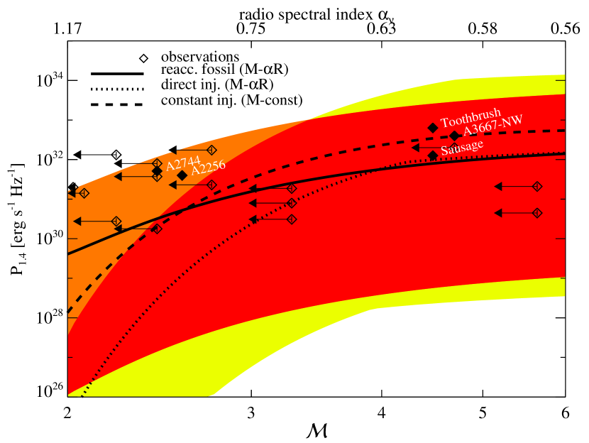
Figure 16: Luminosity from radio relics as a function of Mach number, for reacceleration (solid lines), and direct injection with the ‘M-$\alpha$R’ (dotted lines) and ‘M-const’ model (dashed lines). We also show observations where the intrinsic spectral index can be accurately determined, as in Table 2 (filled diamonds; labelled), and those where we correct for the effects of cooling (open diamonds; upper limits). To bracket the uncertainty in parameters we vary parameters (lower limit, fiducial value, upper limit) and color code the resulting intervals for our reacceleration scenario of fossils (orange), direct injection scenario (yellow) and overlap region (red); shock area $\Psi_{\mathrm{S}}=(0.3,2,4)\,\mathrm{Mpc}^{2}$, downstream temperature $kT_{2}=(1,5,10)\,\mathrm{keV}$, electron number density $n_{\mathrm{e}}=(0.1,1,5)\times 10^{-4}\,\mathrm{cm}^{-3}$, and $B_{2}=(1,5,7)\,\mu$G (magnetic field).

We now make some approximate calculations for the radio relic luminosity function. The differential number density of relics as a function of Mach number can be written as (Ryu et al., 2003):

$$\frac{\mathrm{d}n}{\mathrm{d}\mathcal{M}}=\frac{1}{\Psi_{\mathrm{S}}}\frac{\mathrm{d}S}{\mathrm{d}\mathcal{M}}\,,$$ (37)

where $S$ is the total shock surface area divided by the volume of the simulation box. Thus, $1/S$ has units of length and can be thought of as the mean separation between shocks. We assume a typical area for relic shocks of $\Psi_{\mathrm{S}}=2\,\mathrm{Mpc}^{2}$. We made a fit for the Mach number dependent differential shock surface. It is derived from the shock surface of gas with a pre-shock temperature of $T_{1}\geq 10^{7}$K in a box of size $85\,h^{-1}$Mpc (Kang & Ryu, 2011):

$$\frac{\mathrm{d}S}{\mathrm{d}\mathcal{M}}=10^{-1.015-1.589\mathcal{M}}\,(h^{-1}\,\mathrm{Mpc})^{-1}\,.$$ (38)

The differential number density of radio relics as a function of luminosity is:

$$\frac{\mathrm{d}n}{\mathrm{d}P_{1.4}}=\frac{\mathrm{d}n}{\mathrm{d}\mathcal{M}}\frac{\mathrm{d}\mathcal{M}}{\mathrm{d}P_{1.4}}\,.$$ (39)

where ${\mathrm{d}\mathcal{M}}/{\mathrm{d}P_{1.4}}$ depends on the acceleration model; we use the results of Fig. 16 for reacceleration and direct injection (‘M-$\alpha$R’). The total number of radio relics inside a cosmological box of $(1\,h^{-1}\,\mathrm{Gpc})^{3}$ and with a luminosity above $P_{1.4}$ is:

$$N(>P_{1.4})=(1\,h^{-1}\,\mathrm{Gpc})^{3}\times\int\mathrm{d}P_{1.4}\frac{\mathrm{d}n}{\mathrm{d}P_{1.4}}\,.$$ (40)

The results are shown in Fig. 17. Two features stand out: (1) the reacceleration and direct injection models do not differ significantly in shape, even at the faint end. (2) The model is strongly discrepant with observations for low luminosities. Let us discuss these in turn.

How can we understand the shape of the relic luminosity function? Its features can be broadly understood from the results of Fig. 16. Consider the crosses on the curves for the Kang & Ryu (2011) parametrization in Fig. 17. These mark Mach numbers in unit intervals, starting from 2 (3) for reacceleration (direct injection). The convex shape of the luminosity function is due to the fact that luminosity falls sharply at low Mach number (even for the reacceleration model). Thus, a narrow range in Mach number corresponds to a wide range in luminosity, which ‘stretches out’ N($>P_{1.4}$) to the left at low luminosity and leads to its flat slope, since there are relatively few clusters in an interval $dL$. This amount of ‘stretching’ produced by this non-linear transformation differs between the two models, as evidenced by the different Mach number ticks. However, the small difference in faint end slopes this produces is insufficient to serve as a robust discriminant between models. The offset on the x-axis, due to different limiting luminosities, simply reflects assumptions about asymptotic acceleration efficiencies. The differential luminosity function is similarly poor at distinguishing between models, where the main feature is a sharp peak at the limiting luminosity. The bottom line is that the non-linear mapping between $\mathcal{M}$ and $P_{1.4}$ causes most luminosities to cluster about a characteristic value, which mitigates the efficacy of the luminosity function as a discriminant between models.

The discrepancy of our model predictions with observations is interesting. Such over-prediction of relics also afflicts most current models of the relic luminosity function. Part of the reason may well be that current surveys are simply highly incomplete, particularly at low luminosities. Note also that: (1) the $\mathrm{d}\,S/\mathrm{d}\,\mathcal{M}$ function differs significantly between parametrizations (compare e.g. Ryu et al., 2003; Kang & Ryu, 2011; Araya-Melo et al., 2012), perhaps due to differences in the simulation method, shock finding algorithms, and resolution. Given these differences between simulations, it is perhaps not surprising that they also disagree with observations. Also note that our median distribution function is valid only for the cluster outskirts (which is not singled out by the temperature cut for ${\rm d\,S/d}\,\mathcal{M}$); the distribution function closer in suffers increased Coulomb cooling and has a lower normalization. (2) We have assumed fixed values for most relic parameters, whereas in reality they should have broad distributions, which would produce a tail at high luminosities and smooth out the steep number density function. The parameters we adopt are likely biased by selection effects. For instance, the magnetic field could be highly patchy and inhomogeneous, and only regions which have a strong pre-existing field (to be amplified as a shock) are visible as radio relics.

The above issues are well beyond the scope of this paper, though they deserve careful study in the future. Our main conclusion is that spectrally resolved observations which constrain Mach numbers can distinguish between reacceleration and direct injection, while the relic luminosity function, even with outstanding statistics, cannot.

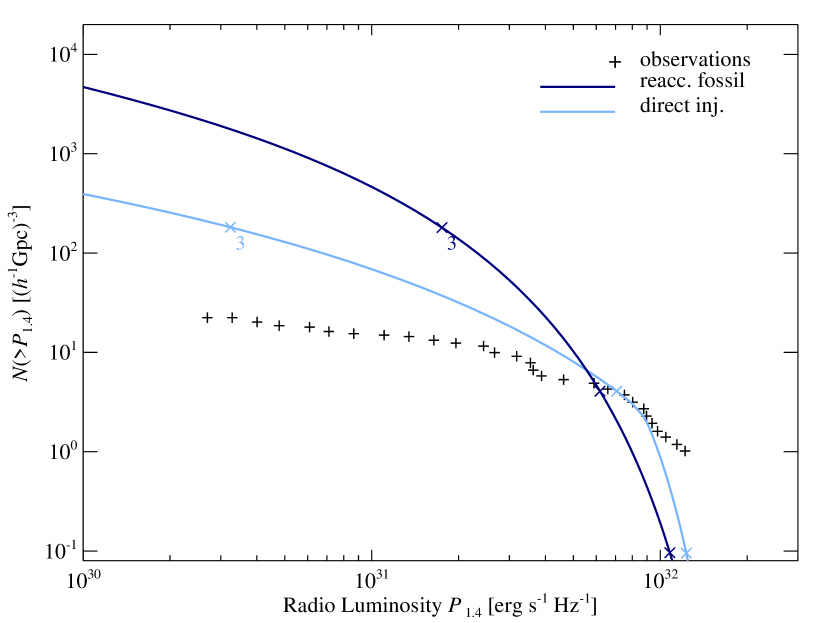
Figure 17: Cumulative number density of radio relics in a $1(h^{-1}\,{\rm Gpc})^{3}$ box. We use the differential shock surface model from Kang and Ryu (equation 38), with reaccelerated fossil electrons and direct injection (‘M-$\alpha$R’ model) and parameters typical for a relic (see Fig. 16). Crosses indicate Mach numbers at unit intervals, starting with the numbers on the left. For comparison, we show the NVSS relic luminosity function (+).

7 Discussion: Insights from Heliospheric Observations

Here, we discuss some uncertainties in our adopted shock physics and numerical method. In particular, we consider our assumptions that the acceleration efficiency plummets at weak shocks, and that the shock surface can be characterized by a single Mach number with little small-scale spatial or temporal structure. We play particular attention to insights gained from heliospheric observations.

7.1 Acceleration Efficiency at Weak Shocks

Are physical processes in the solar system relevant to the ICM? At first blush, the two may appear to differ significantly in their magnetization. While the plasma in the solar wind is strongly magnetized with a plasma beta parameter of $\beta=P_{\mathrm{th}}/P_{B}\sim 0.1-1$ (i.e., the ratio of thermal-to-magnetic pressure, Treumann, 2009), the bulk of the intra cluster plasma is only weakly magnetized with $\beta\gtrsim 50$ as inferred from Faraday rotation measure studies (e.g., in Coma, Bonafede et al., 2010). Those, however, are biased towards the denser core regions and may not be representative of cluster outskirts where relics form. In fact, the plasma beta parameters at the relics’ position are typically an order of magnitude smaller, $\beta\sim 5$. For instance, comparing the limit on the inverse Compton X-ray emission with the measured radio synchrotron emission for the northwest radio relic in A3667 yields a magnetic field estimate of $B\gtrsim 3\,\mu G$ (or equivalently $\beta\lesssim 3$ downstream the shock; Finoguenov et al., 2010). Equating the advection and synchrotron cooling timescales while deprojecting the relic width for the northern relic in the cluster CIZA J2242.8+5301 yields $B\simeq 5-7\,\mu G$ (or equivalently $\beta\simeq 6\pm 3$; van Weeren et al., 2010; Akamatsu & Kawahara, 2011; Ogrean et al., 2013).

What do heliospheric observations tell us about shock acceleration efficiency as a function of Mach number? Extensive spacecraft observations in the solar wind have established that electron acceleration is effectively absent at quasi-parallel weak shocks, i.e. when the upstream magnetic field is approximately parallel to the shock surface normal (Sarris & Krimigis, 1985; Gosling et al., 1989; Krimigis, 1992; Oka et al., 2006; see also a recent review by Treumann, 2009). Electron heating is mainly dominated by conservation of magnetic moment (Feldman, 1985). Quasi-perpendicular weak shocks (with Alvénic Mach numbers $\mathcal{M}_{A}\lesssim 3-4$) show electron acceleration as a result of either shock drift or surfing acceleration, but diffusive shock acceleration appears unlikely (Sarris & Krimigis, 1985; Treumann, 2009). This limits the maximum electron energy to that achievable by shock drift or surfing acceleration, which also depends on the shock ramp width (Lever et al., 2001). Thus, weak shocks in the solar system do not result in efficient electron acceleration (through DSA), consistent with our assumptions for the ICM. One possible interpretation of this is that in order to solve the injection problem of electrons for the DSA mechanism, some process operating under quasi-perpendicular conditions (such as shock drift or surfing acceleration) would be necessary. By contrast, (rare) strong shocks in the solar system show significant local electron acceleration up to particle energies of a few MeV (see GEOTAIL observations of an interplanetary shock with an Alfénic Mach number $\mathcal{M}_{\mathrm{A}}\sim 6$, Shimada et al., 1999), even under quasi-parallel magnetic conditions (as demonstrated by Cassini observations of Saturn’s bow shock with $\mathcal{M}_{\mathrm{A}}\sim 100$, Masters et al., 2013). This may hint at diffusive shock acceleration as the underlying mechanism, in agreement with predictions by theoretical studies (Amano & Hoshino, 2010).

These observations suggest that magnetic geometry strongly impacts acceleration efficiencies—at least locally at the shock where heliospheric observations are providing measurements. In Appendix B, we illustrate how a small variation in a geometric parameter can significantly change the distribution function of fossil electrons. Nonetheless, we do not propagate uncertainties in magnetic geometry across our calculations, and only consider DSA as a source of acceleration. We believe this is justifiable in observed radio relics, on two grounds: (1) The radio spectral slopes are consistent with power-law electron spectra due to diffusive shock acceleration. The high Lorentz factors of $\gamma\sim 10^{4}$ required by the radio data cannot be achieved by shock drift or surfing acceleration. (2) The smoothness of the radio intensity and polarization along the shock surface on scales of $\sim 2$ Mpc argues for a robust acceleration process, independent of the local field geometry. Nonetheless, magnetic geometry is an important caveat in considering the ensemble of possible radio relics: for instance, perhaps only a fraction with favorable geometry are visible.

7.2 Shock Surface

In this paper, we have characterized shocks by a single Mach number (this is particularly important in §6, when we compare our model to observations). Even in the DSA framework, this is an over-simplification (Skillman et al., 2013). More generally, the shock surface is likely to be complex and dynamic. For instance, the crossing of the termination shock in the solar wind by Voyager 2 revealed the presence of a highly dynamic shock surface. Instead of a single crossing of a stationary shock, Voyager 2 passed the shock several times on its ballistic orbit into the heliosheath. The data reveal a complex, rippled, quasi-perpendicular supercritical magnetohydrodynamic shock that undergoes reformation on a scale of a few hours (Burlaga et al., 2008), which corresponds to a characteristic reformation length scale of $\sim 10^{11}\,\mathrm{cm}\sim 0.01$ AU (for a solar wind shock velocity of 300 km s^-1). Supercritical shocks are not capable of generating sufficient dissipation for the retardation, thermalization and entropy increase associated with a shock transition. When the flow exceeds a critical Mach number for a given magnetic obliquity, the supercritical shock starts reflecting particles back upstream. Beyond a second critical Mach number, whistlers accumulate at the shock front and reform periodically (Treumann, 2009). In addition to these microscopic shock reformation mechanisms, there should be macroscopic reformation because of the varying ram pressure and magnetic field fluctuations in the upstream that cause it to reform on gradient length scales of the infalling structures, which likely exhibits a characteristic size spectrum. These are complications well beyond the scope of this paper, but they illustrate possible complexities associated with the shock surface.

More mundanely, our results can depend on the numerical method used to track the injection of CRs. There are known differences in the morphology of accretion shocks in SPH versus mesh-based finite volume methods. Entropy profiles show a sharp peak located around $\sim 2-3\,R_{\mathrm{vir}}$ in mesh-based techniques, while the profiles in SPH simulations—although similar in shape—are smoothed across a sizable larger volume, and the volume-weighted Mach number distribution, particularly for external shocks in low density regions, have different trends in each code (Vazza et al., 2011). However, the Mach number distribution weighted by dissipated energy (which is the most important quantity here) is reassuringly similar for those different numerical schemes owing to the conservative nature of the implemented equations (Vazza et al., 2011). For the resolution used here, we hence do not expect dramatic changes, though direct confirmation is of course preferable.

8 Conclusions

In this paper, we consider giant radio relics in galaxy clusters as the manifestation of reaccelerated fossil relativistic electrons, rather than direct injection from the thermal pool. This idea is not new and has already been proposed in the literature several times (Ensslin et al., 1998; Markevitch et al., 2005; Giacintucci et al., 2008; Kang & Ryu, 2011; Kang et al., 2012; van Weeren et al., 2012, e.g.,). What has been conspicuously missing from the literature is an actual calculation of the fossil electron distribution function, and whether it has the correct shape and amplitude to account for the observations. This paper represents the first attempt to do so. We run a suite of cosmological simulations where cosmic ray electron injection and radiative and Coulomb cooling are tracked in post-processing.

Our principal findings are as follows:

• The fossil CRe population is substantial. Without any fine-tuning, it is at the right level to explain observations.

• Reaccelerated fossil electrons are competitive with direct injection at high Mach numbers, and overwhelmingly dominate by several orders of magnitude at low Mach numbers $\mathcal{M}\lower 2.15277pt\hbox{$\;\buildrel<\over{\sim}\;$}3$. Because it is a relative comparison, this conclusion is fairly robust to the (potentially uncertain) acceleration model, and depends on well-understood structure formation and cooling physics. Given that low Mach number shocks are strongly prevalent in clusters, we predict that LOFAR should find many more unexpectedly bright steep-spectrum radio relics, which cannot be explained by direct injection.

• The fossil distribution function has a generic shape with distinct regimes, where different cooling processes dominate: (1) sub-relativistic Coulomb cooling ($p\lower 2.15277pt\hbox{$\;\buildrel<\over{\sim}\;$}1$), (2) relativistic Coulomb cooling ($1\lower 2.15277pt\hbox{$\;\buildrel<\over{\sim}\;$}p\lower 2.15277pt\hbox{$\;\buildrel<\over{\sim}\;$}10$), (3) quasi-adiabatic ($10\lower 2.15277pt\hbox{$\;\buildrel<\over{\sim}\;$}p\lower 2.15277pt\hbox{$\;\buildrel<\over{\sim}\;$}100$), (4) inverse Compton/synchrotron cooling ($p\lower 2.15277pt\hbox{$\;\buildrel>\over{\sim}\;$}100$). Although fossil electrons peak in number density at $p\sim 1$, due to the sharp change in the nature of Coulomb cooling, electrons at higher energies ($1\lower 2.15277pt\hbox{$\;\buildrel<\over{\sim}\;$}p\lower 2.15277pt\hbox{$\;\buildrel<\over{\sim}\;$}100$ and $10\lower 2.15277pt\hbox{$\;\buildrel<\over{\sim}\;$}p\lower 2.15277pt\hbox{$\;\buildrel<\over{\sim}\;$}10^{4}$ for strong and weak shocks respectively) contribute most to the observationally relevant portion of the reaccelerated spectrum. Cooling times in these regimes are relatively long, and thus it is possible to use simulation outputs with relatively poor time resolution ($\Delta t=$ 100 Myr, 1 Gyr).

• Since both injection and Coulomb cooling change on the (relatively long) dynamical timescale, they can be approximated as steady. We compare a self-similar analytic model where this approximation is made and find excellent agreement with the simulations. This enables extremely rapid estimates. Regime (1), (2) & (4) are in steady-state, while (3) grows monotonically with time.

• There can be up to a factor of $\sim 10$ scatter in fossil electron abundance, depending on a cluster’s merger history; cool core clusters have a lower abundance. Spatial variations within a cluster can also be significant.

Given these considerations, we strongly advocate that fossil electrons be considered a key ingredient in interpreting radio relic observations, rather than an exotic afterthought. Failure to account for the fossil electrons will lead to erroneous conclusions about the nature of particle acceleration at weak shocks. Several extensions immediately suggest themselves. Seed electrons are needed for turbulent reacceleration, as in a prominent model for radio halos (Brunetti & Lazarian, 2007); we are presently studying if fossils from structure formation are adequate. Maps, more detailed and realistic luminosity functions and observational predictions are needed. As discussed in §7.2, confirmation and extension of these results with a grid code would be most welcome. Our main hope is to stimulate others to pursue such lines of inquiry.

Appendix A Cooling

In this section we explain our implementation of cooling in the ”impulsive” scenario in more detail. These are used to evolve the CRe population in our simulations with finite time resolution. We develop analytic expressions which allow very rapid calculations.

A.1 Coulomb cooling

We start by deriving the shift in momentum $p_{\mathrm{i}}$ at time $t_{i}$ to momentum $p_{\mathrm{f}}$ at time $t_{f}$ due to Coulomb cooling by integrating equation (23):

$$-\int_{p_{\mathrm{i}}}^{p_{\mathrm{f}}}\frac{\mathrm{d}p^{\prime}}{b_{\mathrm{C}}(p^{\prime})}\approx\int_{t_{i}}^{t_{f}}\mathrm{d}t\,b_{\mathrm{C}}(t)\equiv F(t_{f},t_{i})\,,$$ (41)

where $b_{\mathrm{C}}(t)=n_{\mathrm{e}}(t)/\tilde{n}$, and $\tilde{n}$ an auxiliary variable introduced to have the correct units. The momentum dependent part is determined by

$$-\int\frac{\mathrm{d}p^{\prime}}{b_{\mathrm{C}}(p^{\prime})}=\int\frac{n_{\mathrm{fix}}\,\mathrm{d}p^{\prime}}{b_{\mathrm{C}}(p^{\prime},t)}$$ (42)

for a fixed electron number density $n_{\mathrm{fix}}=10^{-4}$ cm^-3, and where $b_{\mathrm{C}}(p,t)$ is given by equation (24). The integral over time is performed over snapshots that are discrete in time. Hence, we approximate the time integral for Coulomb cooling between time $t_{i}$ and $t_{f}$ by a discrete sum:

$$F(t_{f},t_{i})\approx\sum_{j=i+1}^{f}\Delta t_{j}\left[b_{\mathrm{C}}(t_{j-1})+b_{\mathrm{C}}(t_{j})\right]/2\,,$$

where $j$ denotes the summation index that run over all snapshots between $t_{i}$ and $t_{f}$. Here we have approximated the time integrated cooling rate between two snapshots by the mean.

First we look at the momentum integral, which we approximate with a simple fit accurate to 20 per cent within $10^{-2}<p<10^{4}$, and $10^{-6}<n_{\mathrm{e}}<10^{-2}$:

$$\int\frac{\mathrm{d}p^{\prime}}{b_{\mathrm{C}}(p^{\prime})} \approx \frac{\kappa\,p^{3}}{\phi+p^{2}}\quad\mathrm{where}\,,$$

$$\kappa = 7.73\times 10^{11}\,\mathrm{s}\,,\quad\mathrm{and}\quad\phi=3.0\,.$$ (44)

We introduce a characteristic momentum for the Coulomb cooling, $p_{\mathrm{Coul}}$, such that

$$\frac{\kappa\,p_{\mathrm{Coul}}^{3}}{\phi+p_{\mathrm{Coul}}^{2}} \equiv \frac{\kappa\,p_{\mathrm{i}}^{3}}{\phi+p_{\mathrm{i}}^{2}}-\frac{\kappa\,p_{\mathrm{f}}^{3}}{\phi+p_{\mathrm{f}}^{2}}=F(t_{f},t_{i})\,,\,\,\mathrm{where}$$ (45)

$$p_{\mathrm{Coul}} = \frac{1}{6}\left\{2^{2/3}\left(J\,F-2\,F^{3}+3^{3/2}\sqrt{K\,J}\right)^{1/3}\right.$$

$$+ \left.2\,F\left[1+\frac{2^{1/3}\,F}{\left(J\,F-2\,F^{3}+3^{3/2}\sqrt{J\,K}\right)^{1/3}}\right]\right\}\,,$$

and

$$K = \phi\,F^{2}\,\mathrm{and}\quad J=27\,\phi+4\,F^{2}\,.$$ (47)

Note that $p_{\mathrm{Coul}}\sim b_{\rm C}(p,t)\Delta t$ in the relativistic regime. The shift in momentum is then given by

$$\Delta p_{\mathrm{Coul}} = p_{\mathrm{f}}-p_{\mathrm{i}}$$ (48)

$$p_{\mathrm{i}} = \frac{1}{6}\left\{2^{2/3}\left(J^{\prime}\,F^{\prime}-2\,F^{\prime 3}+3^{3/2}\sqrt{K^{\prime}\,J^{\prime}}\right)^{1/3}\right.$$

$$+ \left.2\,F^{\prime}\left[1+\frac{2^{\frac{1}{3}}\,F^{\prime}}{\left(J^{\prime}\,F^{\prime}-2\,F^{\prime 3}+3^{\frac{3}{2}}\sqrt{J^{\prime}\,K^{\prime}}\right)^{\frac{1}{3}}}\right]\right\},$$

and

$$F^{\prime} = \frac{p_{\mathrm{f}}^{3}}{\phi+p_{\mathrm{f}}^{2}}+\frac{p_{\mathrm{Coul}}^{3}}{\phi+p_{\mathrm{Coul}}^{2}}\,$$ (50)

$$K^{\prime} = \phi\,F^{\prime 2}\,\mathrm{and}\quad J^{\prime}=27\,\phi+4\,F^{\prime 2}\,.$$ (51)

A.2 Inverse Compton Cooling

We similarly derive the shift in momentum due to inverse Compton cooling by integrating equation (26) from the redshift $z_{i}=z(t_{i})$, where the electrons are injected, to a later time $z_{f}=z(t_{f})$. We define a characteristic momentum $p_{\mathrm{IC}}$, where:

$$\frac{1}{p_{\mathrm{IC}}}\equiv\frac{1}{p_{\mathrm{f}}}-\frac{1}{p_{\mathrm{i}}}\approx\frac{b_{\mathrm{IC},0}}{H_{0}\,p_{\mathrm{f}}^{2}}\int_{z_{f}}^{z_{i}}\frac{(1+z)^{4}\,\mathrm{d}z}{(1+z)\,\sqrt{\Omega_{\mathrm{M}}(1+z)^{3}+\Omega_{\Lambda}}}\,.$$ (52)

Note that $p_{\mathrm{IC}}\sim 1/(b_{\mathrm{IC},0}\,\Delta t)$ for relatively short timescales (where $\Delta t\lesssim 1\,\mathrm{Gyr}$, and $b_{\mathrm{IC},0}$ is given by equation (25)). After the time $\Delta t=t_{f}-t_{i}$ has elapsed, all CRes with a momentum above $p_{\mathrm{IC}}$ have cooled to lower momentum. The shift in momentum is given by $\Delta p_{\mathrm{IC}}=\frac{-p_{\mathrm{f}}^{2}}{p_{\mathrm{IC}}-p_{\mathrm{f}}}$.

A.3 Cooled Distribution Function

Given an initial energy $p_{\mathrm{i}}$ of an electron at time $t_{i}$, equation (23) can be integrated to give the value of $p_{\mathrm{f}}$ at a later time $t_{f}$. The differential population density for relativistic electrons is then given by

$$f_{\mathrm{inj,CRe}}(p_{\mathrm{f}},t_{f},t_{i})=f_{\mathrm{inj,CRe}}(p_{\mathrm{i}},t_{i})\,\left.\frac{\partial p_{\mathrm{i}}}{\partial p_{\mathrm{f}}}\right|_{t_{f}}\,,$$ (53)

where

$$f_{\mathrm{inj,CRe}}(p_{\mathrm{i}},t_{i})=f_{\mathrm{inj,CRe}}(p_{\mathrm{f}}-\Delta p_{\mathrm{IC}}-\Delta p_{\mathrm{Coul}},t_{i})\,,$$ (54)

and

$$\left.\frac{\partial p_{\mathrm{i}}}{\partial p_{\mathrm{f}}}\right|_{t_{f}}=\frac{p_{\mathrm{IC}}^{2}}{\left(p_{\mathrm{IC}}-p_{\mathrm{f}}\right)^{2}}\,-1+$$

$$\left(\frac{p_{\mathrm{f}}}{p_{\mathrm{i}}(p_{\mathrm{Coul}})}\right)^{2}\frac{3\,\phi+p_{\mathrm{f}}^{2}}{\left(\phi+p_{\mathrm{f}}^{2}\right)^{2}}\frac{\left(\phi+p_{\mathrm{i}}(p_{\mathrm{Coul}})^{2}\right)^{2}}{3\,\phi+p_{\mathrm{i}}(p_{\mathrm{Coul}})^{2}}\,.$$ (55)

The total electron spectrum is derived from the sum of all individually cooled injected spectra, starting from the time of injection $t_{i}$ until a later time $t_{f}$,

$$f_{\mathrm{CRe}}(p_{\mathrm{f}},t_{f})=\sum_{j}f_{\mathrm{inj,CRe}}(p_{\mathrm{f}},t_{f},t_{j})\,.$$ (56)

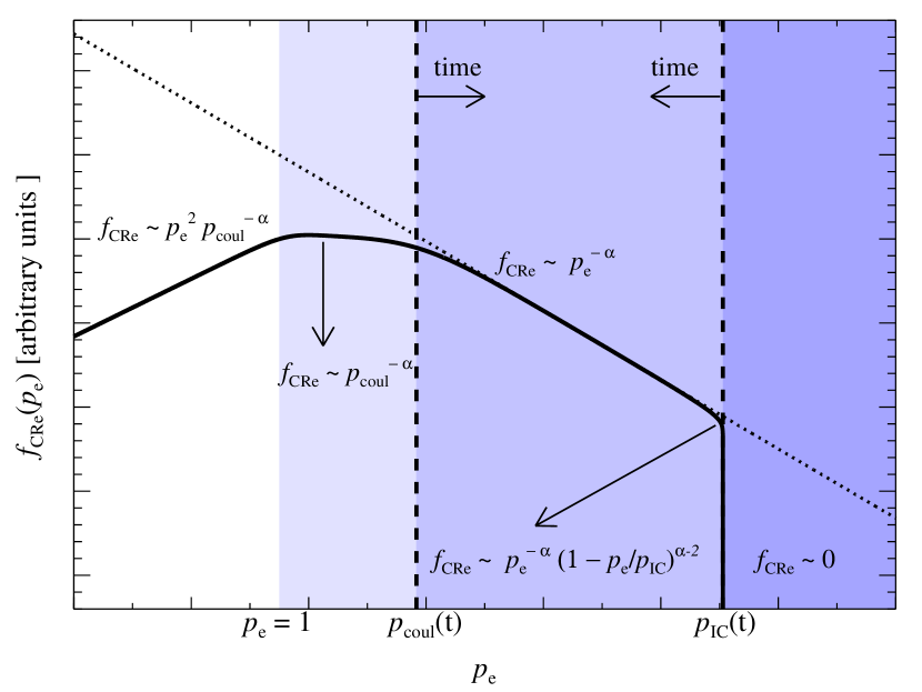
Figure 18: Spectral behavior of the cooled CR electron spectra for different momentum regions. There are several distinct momentum regimes: (1) the low momentum regime ($p\lesssim 1$) is dominated by sub-relativistic Coulomb losses, which cool the CR electrons very efficiently, (2) the less efficient relativistic Coulomb cooling regime ($1\lesssim p\lesssim 10$), (3) the adiabatic regime ($10\lesssim p\lesssim 10^{2}$), which preserves the injected distribution function, and where Coulomb and inverse Compton/synchrotron losses are less important. (4) the inverse Compton/synchrotron cooling regime ($p\gtrsim 10^{2}$). We assume a power-law index of the injected CR electrons of $\alpha=2.5$.

Appendix B Dependence on injection parameter

Here we investigate the importance of the parameter that controls the leakage of the injection process, $\epsilon_{\mathrm{B}}=B_{0}/B_{\perp}$. It is given by the ratio of the amplitude of the downstream MHD wave turbulence, $B_{0}$, to the magnetic field along the shock normal, $B_{\perp}$. The physical range of this parameter is quite uncertain due to complex plasma interactions. We adopt a value of $\epsilon_{\mathrm{B}}=0.23$ in the paper, which corresponds to about a maximum acceleration efficiency of electrons of $\zeta_{\rm e,inj}=0.01$. In Fig. 19 we show how a small variation in this parameter change the distribution function of the fossil CRes. We find a strong dependence on this parameter. However, since $\epsilon_{\mathrm{B}}$ is essentially degenerate with $\zeta_{\rm e,inj}$, it cannot vary too much from our assumed value, as that would conflict with observations of supernova remnants and radio relics.

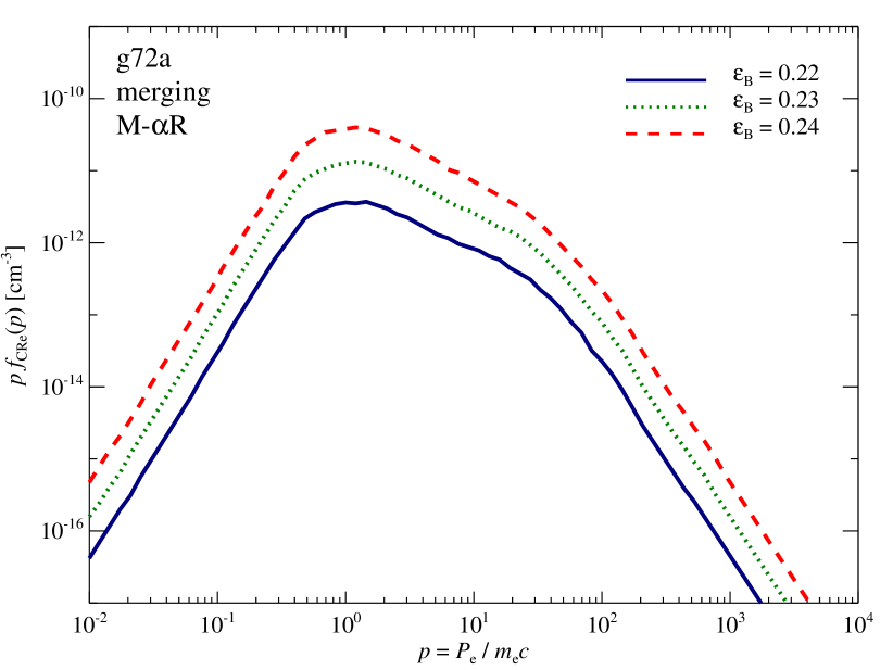
Figure 19: The CR electron dependence on the acceleration parameter $\epsilon_{\mathrm{B}}=B_{0}/B_{\perp}$. We show the median fossil CR electron spectra with full cooling for a large post-merging cluster at $z=0$ in the region between $(0.8-1.0)\,R_{200}$. The spectra are shown for different values of $\epsilon_{\mathrm{B}}$; the value used in the paper $\epsilon_{\mathrm{B}}=0.23$ (green dotted line), $\epsilon_{\mathrm{B}}=0.22$ (blue solid line), and $\epsilon_{\mathrm{B}}=0.24$ (red dashed line).

Appendix C Analytic fit to CR Injection Rate

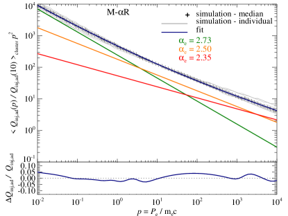
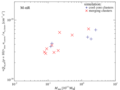
Figure 20: Cosmic ray electron injection rate. We show the median injection rate of CR electrons in the cluster region between $(0.8-1.0)\,R_{200}$ for our sample of 14 simulated galaxy clusters. The upper panel in the left figure shows the spectra as a function of dimensionless CR electron momenta. The injection rate for each cluster is normalized at $p=1$ (grey solid lines). The black crosses show the median of the normalized injection rate across our cluster sample. The blue line shows the best fit triple power-law to the median spectrum, where the red, orange and green lines show each of the fitted power-laws. The bottom left panel shows the difference between the relative fit and the simulation data (blue solid line) which amounts to less than 5 percent. The right figure shows the injection rate, $<Q_{\mathrm{inj,ad}}(p=1,t_{f},t_{i})>_{\mathrm{time}}(n_{\mathrm{e,norm}}/n_{\mathrm{e,cluster}}(t_{f}))$, renormalized with the electron density $n_{\mathrm{e,norm}}=3\times 10^{-5}$ cm^-3, and averaged over time, as a function of galaxy cluster mass $M_{200}$ and cluster morphology. The injection rate for each merging cluster (red crosses) and each cool core cluster (blue $+$) are shown. Note that our limited statistical sample of clusters shows no clear trend with mass.

In this Appendix we present an analytic formula for the time-averaged (over the entire cluster history) CRe injection rate. In the left panel of Fig. 20, we show the injection rate of each cluster as a function of momentum, where we have normalized all curves to have the same value at $p=10$ (adiabatic regime). There is remarkably little difference in the spectral shape, indicating that all clusters have a similar mix of strong and weak shocks. We use a triple power-law fit to capture the spectral shape of the median injection rate over the cluster sample:

$$Q_{\mathrm{inj,ad}}(p,t_{f},t_{i})/Q_{\mathrm{inj,ad}}(10,t_{f},t_{i})=\sum_{i}A_{i}p^{-a_{i}}\,,\,\\$$

where

$$A_{0} =54.0\,,\quad A_{1}=180.0\,,\quad A_{2}=244.8\,,\quad\mathrm{and}$$

$$a_{0} =2.35\,, a_{1}=2.5\,, a_{2}=2.73\,.$$ (57)

This fits to better than 5 per cent over the entire depicted momentum range.

The injection rate at momentum $p=10$ where the electron number density is renormalized, $Q_{\mathrm{inj,ad}}(p=10,t_{f},t_{i})(n_{\mathrm{e,norm}}/n_{\mathrm{e,cluster}})$, is shown in the right panel of Fig. 20. There is no clear trend with cluster mass or morphology. Hence, we adopt a median value of $Q_{\mathrm{inj,ad}}(p=10,t_{f},t_{i})(n_{\mathrm{e,norm}}/n_{\mathrm{e,cluster}}(t_{f}))=5\times 10^{-30}$ cm^-3 s^-1, where we renormalized the density with $n_{\mathrm{e,norm}}=3\times 10^{-5}$ cm^-3.

References

- Akamatsu & Kawahara (2011) Akamatsu H., Kawahara H., 2011, ArXiv:1112.3030
- Amano & Hoshino (2010) Amano T., Hoshino M., 2010, Physical Review Letters, 104, 181102
- Araya-Melo et al. (2012) Araya-Melo P. A., Aragón-Calvo M. A., Brüggen M., Hoeft M., 2012, MNRAS, 423, 2325
- Axford et al. (1982) Axford W. I., Leer E., McKenzie J. F., 1982, A&A, 111, 317
- Battaglia et al. (2009) Battaglia N., Pfrommer C., Sievers J. L., Bond J. R., Enßlin T. A., 2009, MNRAS, 393, 1073
- Bell (1978a) Bell A. R., 1978a, MNRAS, 182, 147
- Bell (1978b) Bell A. R., 1978b, MNRAS, 182, 443
- Berezhko et al. (1994) Berezhko E. G., Yelshin V. K., Ksenofontov L. T., 1994, Astroparticle Physics, 2, 215
- Bertschinger (1985) Bertschinger E., 1985, ApJS, 58, 39
- Blasi (2002) Blasi P., 2002, Astroparticle Physics, 16, 429
- Blasi et al. (2005) Blasi P., Gabici S., Vannoni G., 2005, MNRAS, 361, 907
- Bonafede et al. (2010) Bonafede A., Feretti L., Murgia M., Govoni F., Giovannini G., Dallacasa D., Dolag K., Taylor G. B., 2010, A&A, 513, A30
- Brunetti & Lazarian (2007) Brunetti G., Lazarian A., 2007, MNRAS, 378, 245
- Burlaga et al. (2008) Burlaga L. F., Ness N. F., Acuña M. H., Lepping R. P., Connerney J. E. P., Richardson J. D., 2008, Nature, 454, 75
- Clarke et al. (2011) Clarke T. E., Enßlin T., Finoguenov A., Intema H., Pfrommer C., van Weeren R., Röttgering H., Oonk R., 2011, Mem. Soc. Astron. Italiana, 82, 547
- Drury (1983a) Drury L., 1983a, Space Science Reviews, 36, 57
- Drury (1983b) Drury L. O., 1983b, Reports on Progress in Physics, 46, 973
- Drury & Voelk (1981) Drury L. O., Voelk J. H., 1981, ApJ, 248, 344
- Eichler (1979) Eichler D., 1979, ApJ, 229, 419
- Ellison et al. (2000) Ellison D. C., Berezhko E. G., Baring M. G., 2000, ApJ, 540, 292
- Enßlin & Brüggen (2002) Enßlin T. A., Brüggen M., 2002, MNRAS, 331, 1011
- Enßlin & Gopal-Krishna (2001) Enßlin T. A., Gopal-Krishna 2001, A&A, 366, 26
- Enßlin et al. (2007) Enßlin T. A., Pfrommer C., Springel V., Jubelgas M., 2007, A&A, 473, 41
- Enßlin & Sunyaev (2002) Enßlin T. A., Sunyaev R. A., 2002, A&A, 383, 423
- Ensslin et al. (1998) Ensslin T. A., Wang Y., Nath B. B., Biermann P. L., 1998, A&A, 333, L47
- Feldman (1985) Feldman W. C., 1985, in Tsurutani B. T., Stone R. G., eds, Washington DC American Geophysical Union Geophysical Monograph Series Vol. 35 of Washington DC American Geophysical Union Geophysical Monograph Series, Electron velocity distributions near collisionless shocks. pp 195–205
- Feretti et al. (2012) Feretti L., Giovannini G., Govoni F., Murgia M., 2012, AAPR, 20, 54
- Ferrari et al. (2008) Ferrari C., Govoni F., Schindler S., Bykov A. M., Rephaeli Y., 2008, SSRv, 134, 93
- Finoguenov et al. (2010) Finoguenov A., Sarazin C. L., Nakazawa K., Wik D. R., Clarke T. E., 2010, ApJ, 715, 1143
- Gargaté & Spitkovsky (2012) Gargaté L., Spitkovsky A., 2012, ApJ, 744, 67
- Giacintucci et al. (2008) Giacintucci S., Venturi T., Macario G., Dallacasa D., Brunetti G., Markevitch M., Cassano R., Bardelli S., Athreya R., 2008, A&A, 486, 347
- Gosling et al. (1989) Gosling J. T., Thomsen M. F., Bame S. J., Russell C. T., 1989, JGR, 94, 10011
- Hoeft & Brüggen (2007) Hoeft M., Brüggen M., 2007, MNRAS, 375, 77
- Hoeft et al. (2008) Hoeft M., Brüggen M., Yepes G., Gottlöber S., Schwope A., 2008, MNRAS, 391, 1511
- Jones & Kang (1993) Jones T. W., Kang H., 1993, ApJ, 402, 560
- Jubelgas et al. (2008) Jubelgas M., Springel V., Enßlin T., Pfrommer C., 2008, A&A, 481, 33
- Kang & Jones (1995) Kang H., Jones T. W., 1995, ApJ, 447, 944
- Kang & Jones (2005) Kang H., Jones T. W., 2005, ApJ, 620, 44
- Kang & Ryu (2011) Kang H., Ryu D., 2011, ApJ, 734, 18
- Kang & Ryu (2013) Kang H., Ryu D., 2013, ApJ, 764, 95
- Kang et al. (2012) Kang H., Ryu D., Jones T. W., 2012, ApJ, 756, 97
- Kempner et al. (2004) Kempner J. C., Blanton E. L., Clarke T. E., Enßlin T. A., Johnston-Hollitt M., Rudnick L., 2004, in T. Reiprich, J. Kempner, & N. Soker ed., The Riddle of Cooling Flows in Galaxies and Clusters of galaxies Conference Note: A Taxonomy of Extended Radio Sources in Clusters of Galaxies. pp 335–+
- Keshet (2010) Keshet U., 2010, arXiv:1011.0729
- Krimigis (1992) Krimigis S. M., 1992, SSRv, 59, 167
- Lever et al. (2001) Lever E. L., Quest K. B., Shapiro V. D., 2001, GRL, 28, 1367
- Malkov et al. (2000) Malkov M. A., Diamond P. H., Völk H. J., 2000, ApJL, 533, L171
- Malkov & Völk (1998) Malkov M. A., Völk H. J., 1998, Advances in Space Research, 21, 551
- Markevitch et al. (2005) Markevitch M., Govoni F., Brunetti G., Jerius D., 2005, ApJ, 627, 733
- Masters et al. (2013) Masters A., Stawarz L., Fujimoto M., Schwartz S. J., Sergis N., Thomsen M. F., Retinò A., Hasegawa H., Zieger B., Lewis G. R., Coates A. J., Canu P., Dougherty M. K., 2013, Nature Physics, 9, 164
- Miniati et al. (2001) Miniati F., Ryu D., Kang H., Jones T. W., 2001, ApJ, 559, 59
- Morganti et al. (2010) Morganti R., Rottgering H., Snellen I., Miley G., Barthel P., Best P., Bruggen M., Brunetti G., Chyzy K., Conway J., Jarvis M., Lehnert M., 2010, ArXiv:1001.2384
- Morlino et al. (2009) Morlino G., Amato E., Blasi P., 2009, MNRAS, 392, 240
- Nuza et al. (2012) Nuza S. E., Hoeft M., van Weeren R. J., Gottlöber S., Yepes G., 2012, MNRAS, 420, 2006
- Ogrean et al. (2013) Ogrean G. A., Brüggen M., Röttgering H., Simionescu A., Croston J. H., van Weeren R., Hoeft M., 2013, MNRAS, p. 476
- Oka et al. (2006) Oka M., Terasawa T., Seki Y., Fujimoto M., Kasaba Y., Kojima H., Shinohara I., Matsui H., Matsumoto H., Saito Y., Mukai T., 2006, GRL, 33, 24104
- Orrú et al. (2007) Orrú E., Murgia M., Feretti L., Govoni F., Brunetti G., Giovannini G., Girardi M., Setti G., 2007, A&A, 467, 943
- Parizot et al. (2006) Parizot E., Marcowith A., Ballet J., Gallant Y. A., 2006, A&A, 453, 387
- Pfrommer (2008) Pfrommer C., 2008, MNRAS, 385, 1242
- Pfrommer et al. (2008) Pfrommer C., Enßlin T. A., Springel V., 2008, MNRAS, 385, 1211
- Pfrommer et al. (2007) Pfrommer C., Enßlin T. A., Springel V., Jubelgas M., Dolag K., 2007, MNRAS, 378, 385
- Pfrommer & Jones (2011) Pfrommer C., Jones T. W., 2011, ApJ, 730, 22
- Pfrommer et al. (2006) Pfrommer C., Springel V., Enßlin T. A., Jubelgas M., 2006, MNRAS, 367, 113
- Pinzke & Pfrommer (2010) Pinzke A., Pfrommer C., 2010, MNRAS, 409, 449
- Reynolds (2008) Reynolds S. P., 2008, ARA&A, 46, 89
- Röttgering et al. (1997) Röttgering H. J. A., Wieringa M. H., Hunstead R. W., Ekers R. D., 1997, MNRAS, 290, 577
- Russell et al. (2011) Russell H. R., van Weeren R. J., Edge A. C., McNamara B. R., Sanders J. S., Fabian A. C., Baum S. A., Canning R. E. A., Donahue M., O’Dea C. P., 2011, MNRAS, 417, L1
- Rybicki & Lightman (1979) Rybicki G. B., Lightman A. P., 1979, Radiative processes in astrophysics. New York, Wiley-Interscience
- Ryu et al. (2003) Ryu D., Kang H., Hallman E., Jones T. W., 2003, ApJ, 593, 599
- Sarazin (1999) Sarazin C. L., 1999, ApJ, 520, 529
- Sarris & Krimigis (1985) Sarris E. T., Krimigis S. M., 1985, ApJ, 298, 676
- Schlickeiser (2002) Schlickeiser R., 2002, Cosmic Ray Astrophysics. Berlin: Springer
- Shimada et al. (1999) Shimada N., Terasawa T., Hoshino M., Naito T., Matsui H., Koi T., Maezawa K., 1999, Ap&SS, 264, 481
- Skillman et al. (2011) Skillman S. W., Hallman E. J., O’Shea B. W., Burns J. O., Smith B. D., Turk M. J., 2011, ApJ, 735, 96
- Skillman et al. (2008) Skillman S. W., O’Shea B. W., Hallman E. J., Burns J. O., Norman M. L., 2008, ApJ, 689, 1063
- Skillman et al. (2013) Skillman S. W., Xu H., Hallman E. J., O’Shea B. W., Burns J. O., Li H., Collins D. C., Norman M. L., 2013, ApJ, 765, 21
- Springel (2005) Springel V., 2005, MNRAS, 364, 1105
- Springel & Hernquist (2002) Springel V., Hernquist L., 2002, MNRAS, 333, 649
- Springel et al. (2001) Springel V., Yoshida N., White S. D. M., 2001, New Astronomy, 6, 79
- Treumann (2009) Treumann R. A., 2009, AAPR, 17, 409
- van Weeren et al. (2010) van Weeren R. J., Röttgering H. J. A., Brüggen M., Hoeft M., 2010, Science, 330, 347
- van Weeren et al. (2012) van Weeren R. J., Röttgering H. J. A., Intema H. T., Rudnick L., Brüggen M., Hoeft M., Oonk J. B. R., 2012, A&A, 546, A124
- Vazza et al. (2009) Vazza F., Brunetti G., Gheller C., 2009, MNRAS, 395, 1333
- Vazza et al. (2011) Vazza F., Dolag K., Ryu D., Brunetti G., Gheller C., Kang H., Pfrommer C., 2011, MNRAS, 418, 960
- Zandanel et al. (2012) Zandanel F., Pfrommer C., Prada F., 2012, ArXiv:1207.6410