Measuring the Significance of the Geographic Flow of Music

Abstract

In previous work, our results suggested that some cities tend to be ahead of others in their musical preferences. We concluded that work by noting that to properly test this claim, we would try to exploit the leader-follower relationships that we identified to make predictions. Here we present the results of our predictive evaluation. We find that information on the past musical preferences in other cities allows a linear model to improve its predictions by approx. 5% over a simple baseline. This suggests that at best, the previously found leader-follower relationships are rather weak.

I Reinterpreting the problem of finding leader-follower relationships as a prediction task

In [1], we found that some cities consistently lag others in their musical preferences. The results (such as those depicted in fig. 1) were surprising, indicating for example that Atlanta, Montreal, and Oslo are ahead of other cities in their musical preferences. We were left wondering how meaningful the leader-laggard relationships that we discovered were.

Here we formalize this question in terms of a prediction task. Let us motivate this prediction task with a simple example: suppose we have observed that Toronto lags Montreal in indie music by one week, as in fig. 1. The relationship between Montreal and Toronto suggests that, whenever an indie artist becomes more popular in Montreal, then there should be a substantially increased probability that the same artist will become more popular in Toronto one week later.

Given this notion, a straightforward evaluation procedure suggests itself, based on the following observation: if Montreal really does lead Toronto, then the present and past information we have about Montreal should help us to predict future music trends in Toronto. The stronger this relationship is, the better our predictions will be. If, on the other hand, current information about Montreal only marginally improves our predictions about Toronto’s future, then we can reject our claim that the relationships between Montreal and Toronto is meaningful.

In the next section, we briefly describe the source of our data and formally define the change in a city’s musical preferences as the velocity of a city. Next, we specify the prediction task as well as the linear models that we use for making predictions. Following on, we present the results, which indicate that the past changes in other cities, when utilized by a linear model, predict with an accuracy that is approximately 10% better than predicting that no change will occur in a city’s musical preferences. This finding indicates there is only a low extent to which music flows from one city to another.

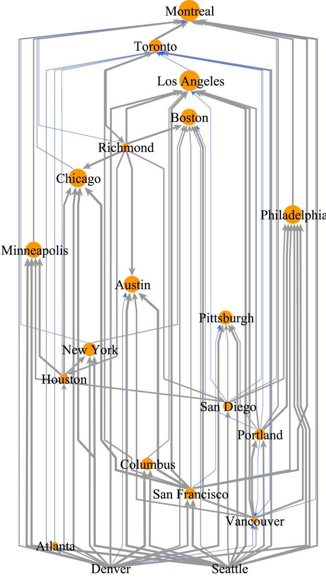
Figure 1: An example of the relationships found in [1]. This network depicts the flow of musical preferences between cities for the genre Indie music. See [1] for details.

Figure 2: Part of the matrix X used for fitting Miami’s linear model. In each row, the values of $y$ is the change in that artists’ popularity in Miami for a given week. The same row in X indicates how that artists popularity changed in other cities in the past.

II Defining a city’s veloctiy in artist space

In this section we provide a brief description of the last.fm data, the preprocessing steps applied to it, and finally motivate and specify the prediction task mentioned in the previous section.

For each of around 200 cities around the world, last.fm publishes a weekly chart which indicates how many unique listerns each of the five hundred most popular artists had each week. For a fuller description of last.fm and the context of the data, see Section II of [1].

The charts data provided by last.fm span every week for more than three years. Let us label the weeks in order as $t_{1},t_{2}\ldots t_{n}$. For each week $t$, we can create a “listeners matrix” such that the rows represent cities, the columns represent artists, and the values indicate the number of unique listers a given artist had in a given city. Let us denote the sequence of these listen matrices as $\mathbf{L}$, and the listeners matrix associated with the $t^{\text{th}}$ week as $\mathbf{L}_{t}$. Thus, $\mathbf{L}_{t,c,a}$ is the number of listeners that artist $a$ had in city $c$ in week number $t$. Note that although any single city can have only 500 non-zero entries in any given week, the matrix as a whole has many thousands of columns, because accross cities and time, the set of 500 most popular artists varies.

A listeners matrix $\mathbf{L}_{t}$ represents cities as points in a high-dimensional “artist space.” If this space is not normalized, then the points which represent large cities with many users (such as London or New York City) will be much further away from the origin than cities with fewer listeners. For our purposes, this is undesirable; instead, we would prefer if two cities that listen to all artists with the same proportion were in the same position in the artist space. For that reason, in each $\mathbf{L}_{t}$, we take the Euclidean norm of each row vector—this ensures that each point’s distance from the origin is one. Let us refer to this normalized version of artist space as $\mathbf{L}^{\prime}$–from here on we will only deal with this normalized version of artist space.

Let us denote the velocity $\mathbf{V}_{t}$ associated with week $t$ to be $\mathbf{L}^{\prime}_{t}$ - $\mathbf{L}^{\prime}_{t-1}$. Let $\mathbf{V}$ denote the sequence of $n-1$ consecutive velocity matrices, $\mathbf{V}_{2}\ldots\mathbf{V}_{n}$.

III Specification of prediction task

Our prediction task is to estimate the future velocity of some target city. The results of [1] indicate that the velocities of some cities consistently lag those of other cities by between 1 and 8 weeks. This implies that when trying to predict the future velocity of some city, the past velocities of other cities should help improve our predictions. If, on the other hand, our predictive model cannot utilize the past velocities of other cities to substantially improve these predictions, then we will have evidence that the the strength of the leader-follower relationship is not sufficient to be useful.

For each city, we will fit two linear models for making predictions, the all history model and the own history model. The all history model will include one coefficient for each (lag size, city) pair and will be fit on a matrix with the form of $\mathbf{X}$ in fig. 2. The own history model will be the same except it will include only information from the city’s own history; it excludes information on the past velocities of other cities. Thus, if the all history model fails to outperform the own history model, then, as stated above, we will conclude that leader-follower relationships are not very meaningful.

As in [1], we will include only the most active US and Canadian cities in the last.fm dataset, and when making a prediction, the model will utilize the previous eight velocities. Each “all history model” model will therefore include 160 coefficients, whereas each “own history model” will have eight. Separately, we perform the same experiment for European cities.

A linear model multplies a matrix X by a vector of coefficients $\beta$ to produce a vector of predictions, $y$, as in fig. 2. We create two $(\textbf{X},y)$ pairs: $(\textbf{X}_{\text{train}},y_{\text{train}})$ and $(\textbf{X}_{\text{test}},y_{\text{test}})$, where the former contains the first two years of data, and the latter contains the final year of data. We use the former to fit the coefficients $\beta$ and the latter to evaluate the quality of the model.

To measure the error of model, we multiply $\textbf{X}_{\text{test}}$ by $\beta$; let us call this product $y_{\text{predict}}$. We then take the root-mean squared error (RMSE) of $y_{\text{test}}$ and $y_{\text{predict}}$. In order to interpret the size of the RMSE, we compare it to the RMSE of a trivial baseline model, which predicts that each city’s velocity will be zero every week (this would be the case if musical preferences did not change). The "linear model error" presented in the tables is in terms of the RMSE of the baseline predictor: a model with 100% indicates has an error size just as large as as the baseline’s error, 50% indicates that the model’s RMSE is half of the baseline’s RMSE.

TABLE I: Prediction accuracy for selected cities in N. America (all)

	Linear model error (pct baseline)
City	Self history	All history	Difference
New York	71.5	68.6	2.9
Phoenix	78.1	74.6	3.5
Vancouver	78.1	74.7	3.4
Pittsburgh	78.0	74.9	3.0
Philadelphia	78.9	75.1	3.9
Minneapolis	79.3	75.1	4.2
Las Vegas	77.2	75.2	2.1
Atlanta	79.8	75.4	4.5
Montreal	78.3	75.6	2.7
Denver	80.5	76.1	4.4
San Diego	80.3	76.1	4.2
Portland	80.4	76.1	4.3
Houston	80.3	76.3	4.0
Columbus	80.0	76.4	3.6
Boston	80.5	76.7	3.9
Austin	81.9	77.0	4.8
San Francisco	82.3	77.3	5.1
Toronto	81.6	78.2	3.5
Seattle	83.5	78.5	5.0
Los Angeles	83.9	78.9	5.0
Chicago	84.1	79.4	4.7
Avg. all	79.9	76.0	3.8
Avg. leaders			3.7
Avg. followers			4.4

IV Results

We run our experiments for all music, and also for a subset of artists who are classified as “indie,” which is a popular genre on last.fm. The results indicate two points. First, none of the results show large improvement over the simple baseline predictor that simply predicts a velocity of zero. For some cities, the RMSE of the “all history” is 12% lower, but that’s the maximum amount of improvement over the baseline, which is not dramatic given that the baseline is quite trivial. Secondly, we see that the “all history” model outperforms the “own history” model, typically achieving twice the improvement over the baseline.

So we are left to conclude that, in the context of a linear model, information about past velocities does not allow one to substantially improve predictions. It is true that a model which includes information about what happens in other cities performs better than a model which has information about only its own history, but even with this improvement, our model outperforms the trivial baseline predictor by only about 10%.

TABLE II: Prediction accuracy for selected cities in N. America (indie)

	Linear model error (pct baseline)
City	Self history	All history	Difference
New York	72.9	70.0	2.9
Phoenix	77.8	74.1	3.7
Las Vegas	76.9	74.7	2.2
Pittsburgh	79.1	75.7	3.5
Portland	80.4	75.7	4.7
Vancouver	79.8	75.8	4.0
Columbus	80.1	75.8	4.3
Denver	81.2	75.9	5.3
San Diego	81.2	76.1	5.1
Philadelphia	80.3	76.3	4.0
Houston	81.1	76.4	4.7
Atlanta	81.7	76.5	5.2
Minneapolis	81.5	77.1	4.5
Seattle	84.1	78.0	6.1
Montreal	80.7	78.4	2.3
Toronto	82.8	78.6	4.1
Boston	82.8	78.6	4.1
Austin	84.1	78.7	5.4
San Francisco	85.2	79.3	5.9
Los Angeles	85.8	80.5	5.3
Chicago	87.2	81.0	6.2
Avg. all	81.3	76.8	4.5
Avg. leaders			4.3
Avg. followers			5.1

TABLE III: Prediction accuracy for selected cities in Europe (All)

	Linear model error (pct baseline)
City	Self history	All history	Difference
Dublin	70.2	67.4	2.8
Munich	76.9	74.1	2.8
Vienna	78.3	75.5	2.8
Bristol	79.9	75.6	4.3
Hamburg	78.9	76.6	2.3
Birmingham	80.9	77.2	3.7
Leeds	81.5	77.6	3.8
Berlin	80.3	77.8	2.5
Barcelona	81.4	77.8	3.6
Cracow	80.5	77.8	2.7
Milan	80.9	78.6	2.3
Manchester	83.9	79.0	4.9
Madrid	84.8	81.4	3.5
Paris	83.8	81.5	2.3
Brighton	87.7	82.6	5.1
Warsaw	86.2	84.1	2.1
London	92.5	87.8	4.7
Stockholm	90.9	88.7	2.2
Oslo	92.9	91.3	1.6
Avg. all	82.8	79.6	3.2
Avg. leaders			2.7
Avg. followers			3.1

TABLE IV: Prediction accuracy for selected cities in Europe (indie)

	Linear model error (pct baseline)
City	Self history	All history	Difference
Dublin	69.9	66.7	3.2
Bristol	78.8	74.7	4.1
Munich	78.6	75.2	3.5
Birmingham	79.5	75.8	3.7
Vienna	81.0	77.0	4.0
Manchester	82.1	77.4	4.7
Hamburg	80.6	77.8	2.8
Berlin	81.4	78.6	2.8
Leeds	81.8	78.8	2.9
Brighton	83.7	79.8	3.9
Barcelona	83.7	79.8	3.9
Milan	84.7	81.6	3.1
Cracow	86.7	82.6	4.1
Paris	86.3	82.6	3.7
Madrid	87.3	82.9	4.5
Stockholm	90.5	87.0	3.5
London	91.7	87.2	4.5
Warsaw	93.1	89.0	4.0
Oslo	93.7	91.0	2.8
Avg. all	83.9	80.3	3.7
Avg. leaders			3.4
Avg. followers			3.8

V Discussion: relating our current findings to those of [1]

In [1], we found that some cities consistently lag others in their musical preferences. We were left wondering how meaningful the leader-laggard relationships that we discovered were. Here we have formalized this question by re-casting our data analysis as a prediction problem. We model a city’s future change in its musical preferences as a linear combination of previous changes. If the model has access only to its own past velocities, the model’s error is about 80% of the error associated with a trivial model (predict a change of zero). When we allow the model to also include the past changes in other cities, the model’s error drops by an additional 3-4%. These findings indicate that the previous changes of other cities are only weakly related to any city’s future change in musical preferences.

Let us now consider how our findings here relate to [1]. One could argue that the linear models we use in this work are not comparable to the methods used in [1]. Indeed, in that work, there was no explicit model—we simply adapted a method proposed in [2]. However, one could argue that the network diagrams in [1] suggest a sort of “implicit model.” While it’s reasonable to assume that the implicit model is a linear model, it probably does not allow for negative coefficients. Thus the linear model we use here (which does allow negative coefficients) is more expressive than the concepts of flow that we considered in [1]. However, even with the more flexible model considered here, we were not able to make great predictions. This suggests that the model implicit in [1] would have been at least as bad, and likely worse, at predicting changes in musical preferences. In fact, we also tried using linear models whose coefficients were constrained to be positive, but these models always performed substantially worse. Thus, our evaluation here can only put an upper bound on the quality of the predictions possible with the relationships we proposed in [1].

Can we find any traces of a connection behind our specific findings in [1] and our findings here? Are the leader-follower relationships we identified in that paper not only weak, but also spurious? Ideally we would be able to compare the leader follower relationships identified in that previous work with the ones identified here. However, because interpreting the coefficients of linear models is not straigtforward, there is no clear way of identifying the leader-follower relationships present in the linear models developed here.

We can still try to find some indirect connections between the two sets of results. It is reasonable to assume that for cities which are laggards, i.e., low down in diagrams like fig. 1, information on what happens in other cities should especially helpful. In other words, if a particular city is a laggard, then its future changes will tend to be more determined by the past changes in other cities, whereas if a city is a leader, then such information will be less useful. Thus laggard cities (highligted in red in the tables) should benefit more tha leading cities (highlighted in green). In all four cases (All music and indie music in both N. America and Europe) the average benefit of the 6 laggard cities was greater than the corresponding benefit for the leading cities. Thus, it appears that we can make some connection between our findings here and our findings in [1].

References

- [1] C. Lee and P. Cunningham, “The geographic flow of music,” Arxiv preprint arXiv:1204.2677, 2012.
- [2] M. Nagy, Z. Akos, D. Biro, and T. Vicsek, “Hierarchical group dynamics in pigeon flocks.” Nature, vol. 464, no. 7290, pp. 890–3, Apr. 2010.