Constraints on the Synchrotron Emission Mechanism in GRBs

Abstract

We reexamine the general synchrotron model for GRBs’ prompt emission and determine the regime in the parameter phase space in which it is viable. We characterize a typical GRB pulse in terms of its peak energy, peak flux and duration and use the latest Fermi observations to constrain the high energy part of the spectrum. We solve for the intrinsic parameters at the emission region and find the possible parameter phase space for synchrotron emission. Our approach is general and it does not depend on a specific energy dissipation mechanism. Reasonable synchrotron solutions are found with energy ratios of $10^{-4}<\epsilon_{B}/\epsilon_{e}<10$, bulk Lorentz factor values of $300<\Gamma<3000$, typical electrons’ Lorentz factor values of $3\times 10^{3}<\gamma_{e}<10^{5}$ and emission radii of the order $10^{15}\mbox{cm}<R<10^{17}$cm. Most remarkable among those are the rather large values of the emission radius and the electron’s Lorentz factor. We find that soft (with peak energy less than 100KeV) but luminous (isotropic luminosity of $~{}1.5\times 10^{53}$) pulses are inefficient. This may explain the lack of strong soft bursts. In cases when most of the energy is carried out by the kinetic energy of the flow, such as in the internal shocks, the synchrotron solution requires that only a small fraction of the electrons are accelerated to relativistic velocities by the shocks. We show that future observations of very high energy photons from GRBs by CTA, could possibly determine all parameters of the synchrotron model or rule it out altogether.

1 Introduction

GRBs’ non thermal spectrum has lead to the suggestion that both the prompt and the afterglow are produced by synchrotron emission of relativistic electrons (Katz, 1994; Rees and Mészáros, 1994; Sari et al., 1996, 1998). There is reasonable agreement between the predictions (Sari et al., 1998) of the synchrotron model and afterglow observations (Wijers and Galama, 1999; Granot et al., 1999, 2002; Panaitescu and Kumar, 2001; Nousek et al., 2006; Zhang et al., 2006). However, the situation concerning the prompt emission is more complicated.

The observations of many bursts whose lower spectral slope is steeper than the “synchrotron line of death” (Crider et al., 1997; Preece et al., 1998, 2002) pose a serious problem to synchrotron emission. This has motivated considerations of photospheric thermal emission (Eichler $\&$ Levinson, 2000; Mészáros $\&$ Rees, 2000; Peer et al., 2006; Rees $\&$ Mészáros, 2005; Giannios, 2006; Thompson et al., 2007; Ryde and Peer, 2009), in which thermal energy stored in the bulk is radiated in the prompt phase at the Thomson photosphere and the high energy tail is produced by inverse Compton. While this model yields a consistent low energy slope it has its own share of problems. Most notably Vurm et al. (2012) have recently shown that unless the outflow is moving very slowly no known mechanism can produce the needed soft photons. Furthermore, it is not clear how the high energy GeV emission can be produced within an optically thick regime (Vurm et al., 2012a). On the other hand, observations of some bursts, e.g. GRB 080916C in which there is a strong upper limit on the thermal component (Zhang et al., 2009), or GRBs: 100724B, 110721A, 120323A, where a thermal component was possibly detected but with only a small fraction ($5-10\%$) of the total energy in the thermal component (Guiriec et al., 2011, 2012; Axelsson et al., 2012) and other bursts whose spectral slopes is consistent with synchrotron suggest that for some bursts synchrotron might be a viable model. In fact, in all cases that involve Poynting flux outflows that are Poynting flux dominated at the emitting region synchrotron is inevitable and possibly dominant (Beniamini $\&$ Piran, 2013). As such it is worthwhile to explore the conditions needed to generate the observed prompt emission via synchrotron .

To examine the conditions for synchrotron to operate, we consider a general model that follows the spirit of Kumar $\&$ McMahon (2008). We don’t make any specific assumptions concerning the details of the energy dissipation process or the particle acceleration mechanism. Instead we assume that relativistic electrons and magnetic fields are at place within the emitting region, that is moving relativistically towards the observer. We examine the parameter space in which these electrons emit the observed radiation via synchrotron while satisfying all known limits on the observed prompt emission. We use a simple “single-zone” calculations that do not take into account the blending of radiation from different angles or from different emitting regions (reflecting matter moving at different Lorentz factors), but for the purpose of obtaining the rough range of relevant parameters this is sufficient.

We characterize the conditions within the emitting region by six parameters: the co-moving magnetic field strength, $B$, the number of relativistic emitters, $N_{e}$, the ratio between the magnetic energy and the internal energy of the electrons, $\epsilon\equiv\epsilon_{B}/\epsilon_{e}$, the bulk Lorentz factor of the emitting region, $\Gamma$, the minimal electrons’ Lorentz factor in the source frame, $\gamma_{m}$ and the ratio between the shell crossing time and the angular timescale, $k$. We then characterize a single, “typical”, GRB pulse, which is the building block of the GRB lightcurve, by three basic quantities: the peak (sub-MeV) frequency, the peak flux and the duration. We compare the first two, the observed peak (sub-MeV) frequency and the peak flux with the predictions of the synchrotron model and we use the observed duration of the pulse to limit the angular time scale (Sari and Piran, 1997a). The synchrotron solution is incomplete without a determination of the accompanying synchrotron self-Compton (SSC) emission, which influences the efficiency of the synchrotron emission. Furthermore, the observations of the high energy SSC emission poses additional constraints on the emitting region. We describe, therefore, a self-consistent synchrotron self-Compton solution.

Three additional constraints should be taken into account (see also Daigne et al., 2011). First, energy considerations pose a strong lower limit on the efficiency. The energy of the observed sub-MeV flux, is huge and already highly constraining astrophysical models. Thus, to avoid an “energy crisis”, the emission process must be efficient and emit a significant fraction of the available energy in the sub-MeV band. Second, the emission region cannot be optically thick. Additionally, the LAT band (100 MeV- 300 GeV) GeV component is significantly weaker in most GRBs than the sub-MeV peak (Granot et al., 2009, 2010; Beniamini et al., 2011; Guetta et al., 2011; Ackermann et al., 2012). We combine these three conditions and constrain the possible phase space in which synchrotron can produce the prompt emission.

The paper is organized as follows. We describe in §2 the basic concepts of the model, discussing the observations in §2.1 and the structure of the emitting region and the parameter phase space in §2.2. In §3 we describe the synchrotron equations (§3.1), their solutions (§3.2), the constraints from the accompanying SSC (§3.3), the implications of the results (§3.4) and energy and efficiency constraints (§3.5). We continue with a discussion of specific issues concerning the (i) expected spectral slopes and possibilities to alleviate the issue of the “synchrotron line of death” (§3.6) and (ii) the narrow $E_{peak}$ distribution (§3.7). In §4, we deviate from the general philosophy of the paper and we discuss synchrotron emission within the context of the popular internal shocks framework. We turn, in §5, to the implications of the pair creation limits from observed GeV emission for the synchrotron model. In §6 we briefly discuss the possibilities of detecting GRBs with CTA, and their implications on the model at hand.

2 The Global Picture

2.1 The observations

Limits on the optical (Roming et al., 2006; Yost et al., 2007; Klotz, 2009), x-ray (O’Brien et al., 2006), GeV (Ando et al., 2008; Guetta et al., 2011; Beniamini et al., 2011; Ackermann et al., 2012) and TeV (Atkins et al., 2005; Albert et al., 2006; Aharonian et al., 2009) emission during the prompt phase of GRBs, demonstrate that the observed sub-MeV peak carries most of the GRB’s energy. The only (unlikely) possibilities that have not been ruled out are either an extremely strong and sharp peak between 10-100eV or a peak at extremely high energies above the TeV range. Therefore, we associated the sub-MeV peak with the peak of the synchrotron emission.

We consider the typical observations after redshift corrections, i.e. in the host galaxy frame which we denote as “the source frame” (as opposed to “the observer frame”). The basic observables are: the peak frequency: $h\nu_{peak}\equiv h\nu_{peak,obs}\times(1+Z)$ (300KeV), the duration of a typical pulse, $t_{p}\equiv t_{p,obs}/(1+Z)$ (0.5 sec) and the peak flux, $F_{\nu_{peak}}\equiv F_{\nu_{peak,obs}}/(1+Z)$ ($1.5\times 10^{-26}\mbox{erg}/\mbox{cm}^{2}\mbox{sec Hz}$). With these definitions we remove the $(1+Z)$ dependence from the equations, and the only remaining dependence on redshift is through the luminosity distance, relating the flux and luminosity. All three quantities vary from pulse to pulse and the values in brackets denote the canonical values that we use here. These three observations together with a typical luminosity distance, $d_{L}=2\times 10^{28}$ cm (or $z=1$) correspond to an isotropic equivalent luminosity of $L_{iso}\approx 2\times 10^{52}$erg/sec. It has been suggested that $E_{peak}$ and $L$ satisfy: $L_{p}=10^{52.43}({E_{peak}(1+z)}/{355\mbox{KeV}})^{1.6}$erg/sec (Yonetoku et al., 2010), we therefore choose $\nu_{peak}$ and $L_{p}$ such that they are compatible with this relation. In §3.7 we explore the dependence of the synchrotron model on this choice and look at 4 representative “GRB types”. An additional observation that we use is the limit on the total flux observed in the LAT band (30 MeV-300 GeV), which is at most 0.13 of the GBM (8KeV-40MeV) flux (Beniamini et al., 2011; Ando et al., 2008; Guetta et al., 2011; Ackermann et al., 2012).

2.2 The emitting region

The general model requires a relativistic jet, traveling with a Lorentz factor $\Gamma$ with respect to the host galaxy with a half opening angle of $\theta$, at a distance $R$ from the origin of the explosion and with a kinetic energy $E_{tot}$ in the source frame. The source can be treated as spherically symmetric as long as $\Gamma^{-1}<\theta$ which is expected to hold during the prompt phase, in which $\Gamma\geqslant 100$ (Fenimore et al., 1993; Woods and Loeb, 1995; Piran, 1995; Sari and Piran, 1999). We therefore do not solve for $\theta$ and use isotropic equivalent quantities throughout the paper. An upper limit on the emitting radius is given by the variability time scale, $t_{p}\geqslant t_{ang}\equiv R/(2c\Gamma^{2})$. We define a dimensionless parameter $k$ such that $kR/G^{2}$ is the shell’s width:

$$t_{cross}\equiv\frac{kR}{2c\Gamma^{2}}=kt_{ang}.$$ (1)

With this definition, the pulse duration is:

$$t_{p}\equiv\frac{(k+1)R}{2c\Gamma^{2}}.$$ (2)

Clearly, for $k=1$ the pulse width is determined by angular spreading.

We consider a single-zone model in which the different properties of the emitting region are constant throughout the zone. Notice that the single-zone approach cannot test spectral evolution, and becomes less accurate as $k$ increases. Initially, the emitting region consists of either an electron-proton or an electron-positron plasma. The numbers of protons and positrons are denoted by $N_{p}$ and $N_{e+}$ respectively. Due to electrical neutrality, the number of electrons is $N_{p}+N_{e+}$. After the gamma-rays are produced, annihilating high energy photons may result in extra electrons and positrons. We denote the number of pairs created in this way by $N_{pairs}$ (typically these particles are less energetic than the original population of emitting particles). Altogether, there are $N_{tot}=N_{p}+2N_{e+}+2N_{pairs}$ electrons and positrons in the flow. the number of electrons is always larger than the number of positrons except for the case of an initial pair dominated outflow, where they are equal. Therefore, to simplify the presentation, we use hereafter ”electrons” instead of the more accurate but cumbersome ”electrons and positrons”. In the fast cooling regime, the typical synchrotron cooling time of a relativistic electron is shorter than the pulse duration and thus the instantaneously emitting particles are much less than the total number of emitting particles during one pulse (see Fig.1). The emitting electrons are characterized by $X_{ins}\leq 1$ which is defined to be the ratio between the number of instantaneously emitting electrons and the overall number of relativistic electrons emitting during the entire pulse (A concise definition of all these particle numbers is given in table 1).

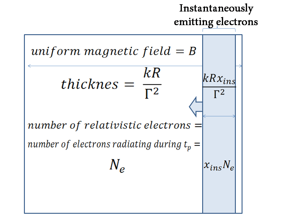
Figure 1: A schematic representation of the single zone model. The model assumes that the physical conditions are uniform throughout the emitting region. Due to the short cooling time by radiation (compared with the pulse duration) the instantaneously emitting particles reside in a thinner slab than the overall population.

Notation	Description
$N_{tot}$	The total number of electrons (and positrons)
$N_{pairs}$	The number of pairs created by annihilating high energy photons
$N_{p}$	The number of protons in the initial flow
$N_{e+}$	The number of positrons in the initial flow
$N_{e}$	The number of relativistic electrons (and positrons) radiating during one pulse
$x_{ins}$	Ratio between instantaneously emitting electrons (and positrons) and $N_{e}$

Table 1: Different particle numbers used in the text.

Excluding the original pairs that may reside in the initial flow and are accounted for by $N_{e+}$

The relativistic electrons have a power-law distribution of energies:

$$\frac{dN_{e}}{d\gamma}=C(\frac{\gamma}{\gamma_{m}})^{-p},$$ (3)

(where C is a normalization constant) which holds for $\gamma_{m}<\gamma<\gamma_{Max}$. Based on theory, we expect $p$ to be of the order $p\sim 2.5$ (Achterberg et al., 2001; Bednarz et al., 1998; Gallant $\&$ Achterberg, 1999). Indeed this result has been confirmed observationally both from the GRB prompt and afterglow phases (Sari and Piran, 1997b; Panaitescu and Kumar, 2001). $\gamma_{Max}$ arises, most likely, due to Synchrotron losses at the energy where the acceleration time equals to the energy loss time (de Jager, 1996):

$$\gamma_{Max}=4\times 10^{7}fB^{-1/2},$$ (4)

where $f$ is a numerical constant of order unity which encompasses the details of the acceleration process and $B$ is measured in Gauss. In a shock-acceleration scenario this depends on the amount of time the particle spends in the downstream and upstream regions (Piran $\&$ Nakar, 2010; Barniol Duran $\&$ Kumar, 2011). The total internal energy of the electrons is then (primes denote the co-moving frame):

$$E_{e}^{\prime}=\frac{p-1}{p-2}\gamma_{m}N_{e}m_{e}c^{2}\equiv\epsilon_{e}E_{int}^{\prime},$$ (5)

where $E_{int}^{\prime}$ is the energy of the flow dissipated into internal energy and the ratio of the total energy in these relativistic electrons to the total internal energy is denoted by $\epsilon_{e}$. Notice that $\epsilon_{e}$ does not necessarily reflect the ratio of instantaneous energy of the relativistic electrons to the total energy, which could be much smaller.

The magnetic field, $B$, is assumed to be constant over the entire emitting region. Its energy is:

$$E_{B}^{\prime}=\frac{B^{2}}{8\pi}4\pi R^{2}\frac{kR}{\Gamma}\equiv\epsilon_{B}E_{int}^{\prime}=\epsilon E_{e}^{\prime},$$ (6)

where $kR/\Gamma$ is the thickness of the shell in the co-moving frame and $\epsilon_{B}$ is the fraction of magnetic to internal energy. In this case, for a Baryoninc dominated flow, $\epsilon_{B}+\epsilon_{e}\leqslant 1$. Whereas, in a Poyinting flux dominated jet, one can imagine a situation in which at first the energy is stored within the magnetic fields, and only later it is dissipated and transferred to the electrons. Within the definitions we use here, this means that $\epsilon_{e}+\epsilon_{B}\lesssim 2$.

Overall, we find that six independent parameters define the synchrotron solution These are: the co-moving magnetic field strength, $B$, the number of relativistic electrons, $N_{e}$, the ratio between the magnetic energy and the kinetic energy of the electrons, $\epsilon\equiv\epsilon_{B}/\epsilon_{e}$, the bulk Lorentz factor of the jet with respect to the GRB host galaxy, $\Gamma$, the minimum electrons’ Lorentz factor in the source frame, $\gamma_{m}$, and the ratio between the shell crossing time and the angular timescale, $k$. The first three observables: the spectral peak, the peak luminosity and the pulse duration, described in §2.1, reduce the number of free parameters from six to three, which we choose as: ($\epsilon_{B}/\epsilon_{e},\Gamma,k$). The other constraints limit the allowed regions within this parameter space.

3 Detailed method and results

3.1 The synchrotron equations

The typical synchrotron frequency and power produced by an electron with a Lorentz factor $\gamma_{e}$ are: (Rybicki and Lightman, 1979; Wijers and Galama, 1999)

$$\nu_{syn}=\Gamma\gamma_{e}^{2}\frac{q_{e}B}{2\pi m_{e}c},$$ (7)

$$P(\gamma_{e})=\frac{4}{3}\sigma_{T}c\Gamma\gamma_{e}^{2}\frac{B^{2}}{8\pi},$$ (8)

where $\Gamma$ is the Lorentz factor of the bulk and $\sigma_{T}$ is the Thomson cross-section. When the electrons have a power-law distribution of energies above some $\gamma_{m}$ there are two typical breaks in the spectrum. The first is the synchrotron frequency of a typical electron, $\nu_{m}\equiv\nu_{syn}(\gamma_{m})$. The second is the cooling frequency, the frequency at which electrons cooling on the pulse time-scale, radiate:

$$\nu_{c}=\frac{18\pi q_{e}m_{e}c}{\sigma_{T}^{2}B^{3}\Gamma t_{p}^{2}{(1+Y_{0})}^{2}},$$ (9)

where $Y_{0}$ is the relative energy loss by IC as compared with synchrotron for $\gamma_{e}=\gamma_{c}$.

The peak of the synchrotron $\nu F_{\nu}$ is at $max[\nu_{c},\nu_{m}]$ (Sari et al., 1998). We identify this peak with the observed sub-MeV peak. For $\nu_{c}<\nu_{m}$, the ”typical” electrons are fast cooling and rapidly dispose of all their kinetic energy, while for $\nu_{c}>\nu_{m}$ the electrons are slow cooling and the typical electrons do not emit all their energy which is eventually lost by adiabatic cooling. We consider fast cooling solutions (or marginally fast) for the prompt emission.

The maximal spectral flux, at $min[\nu_{c},\nu_{m}]$ is given by combining Eqns. 7, 8:

$$F_{\nu,max}=\frac{m_{e}c^{2}\sigma_{T}\Gamma BN_{e}}{3q_{e}4\pi d_{L}^{2}}.$$ (10)

For $\nu_{c}<\nu_{m}$, this is the flux at $\nu_{c}$ and the peak of $F_{\nu}$. However, in the fast cooling regime the flux between $\nu_{c}$ and $\nu_{m}$ varies as $F_{\nu}\propto\nu^{-1/2}$ and the peak of $\nu F_{\nu}$ is at $\nu_{m}$:

$$F_{\nu,m}=F_{\nu,max}(\frac{\nu_{m}}{\nu_{c}})^{-1/2}=\frac{m_{e}c^{2}\sigma_{T}\Gamma Bx_{ins}N_{e}}{3q_{e}4\pi d_{L}^{2}(1+Y_{0})},$$ (11)

where the factor $x_{ins}/(1+Y_{0})\equiv(\nu_{c}/\nu_{m})^{1/2}$ accounts for the fact that only $x_{ins}$ of the relativistic electrons are instantaneously emitting and only $1/(1+Y_{0})$ of their energy loss is by synchrotron (the rest is by the accompanying SSC). In the fast cooling regime, the electrons cool on a shorter timescale than the pulse duration and several consecutive cooling processes may be needed to account for the comparatively long pulse duration. Eq. 11 can be understood in terms of the cooling time of the electrons, $t_{c}$, the time it takes the electrons to radiate (by synchrotron and IC) their kinetic energy:

$$t_{c}(\gamma_{e})=\frac{\Gamma\gamma_{e}m_{e}c^{2}}{\frac{4}{3}c\sigma_{T}\gamma_{e}^{2}\Gamma^{2}\frac{B^{2}}{8\pi}(1+Y_{0})}.$$ (12)

$t_{c}(\gamma_{e})$ is declining as a function of $\gamma_{e}$. Therefore it is maximal for $\gamma_{m}$, and after a time $t_{c}(\gamma_{m})$ all of the electrons have cooled significantly. Combining Eqs. 7, 9 and 12 gives: $t_{c}(\gamma_{m})/t_{p}=(\nu_{c}/\nu_{m})^{1/2}$. It follows that: $x_{ins}/(1+Y_{0})=t_{c}(\gamma_{m})/t_{p}$, which tells us that indeed only the instantaneously synchrotron emitting electrons contribute to the peak of $\nu F_{\nu}$.

Given the spectrum, the source must be optically thin for scatterings:

$$\tau=\frac{N_{tot}\sigma_{T}}{4\pi R^{2}}\lesssim 1,$$ (13)

where $N_{tot}=N_{e}+2N_{pairs}$ is the total number of electrons and positrons in the flow. $N_{tot}$ is composed of two components. The first, $N_{e}$, is calculated from the peak flux. Notice that in principle there could be additional non-relativistic electrons in the initial flow that although they don’t contribute to the radiation, they can be important due to their effect on the optical depth. We return to this point in §3.2. The second, $2N_{pairs}$, is the electron-positron pairs created by annihilation of the high energy photons . $N_{pairs}$ is derived by considering the optical depth for pair creation (Lithwick $\&$ Sari (2001)):

$$\tau_{\gamma,\gamma}(\nu)=\frac{\frac{11}{180}\sigma_{T}n_{>\nu,an}}{4\pi R^{2}}\lesssim 1$$ (14)

where $n_{>\nu,an}$ is the number of photons in the source with enough energy to annihilate the photon with frequency, $\nu$. The frequency $\nu_{thick}(\Gamma)$, is defined as the (source frame) photon frequency at which $\tau_{\gamma,\gamma}(\nu_{thick})=1$. Therefore, $N_{pairs}$ equals the number of photons above $\nu_{thick}(\Gamma)$.

A more detailed calculation of the pair creation opacity has to take care of the details of the radiation field in the source (Granot et al., 2008; Hascoët et al., 2012). There could in principle be a numerical factor in Eq. 14 of order $\sim 0.01-0.1$ (Granot et al., 2008; Hascoët et al., 2012; Vurm et al., 2012) This in turn, would lower the minimum requirement on $\Gamma$. However: $\Gamma\propto\tau^{\frac{1}{6}}$, which means that the change in the lower limit of $\Gamma$ in the exact calculation, will only be of order 0.5-0.7.

3.2 A synchrotron solution for the MeV peak

We solve the synchrotron Eqns. described in §3.1 and reduce the 6D parameter space described in §2.2 to a 3D parameter space defined by ($\epsilon,\Gamma,k$). We then consider three constraints that limit the allowed regions within this parameter space. In §5 we discus further constraints on this parameter space that arise from pair creation opacity limits.

Solving Eqns. 2, 6, 7, 9 and 11 we find:

$$B=2\times 10^{4}(1+Y_{0})^{1/2}\Gamma_{2}^{-3}(\epsilon)^{1/2}k^{-1/2}(k+1)^{3/2}\nu_{p,300}^{1/2}t_{p,.3}^{-1}F_{-26.2}^{1/2}d_{28}\mbox{ Gauss},$$ (15)

$$x_{ins}=1.1\times 10^{-5}(1+Y_{0})^{-7/4}\Gamma_{2}^{4}(\epsilon)^{-3/4}k^{3/4}(k+1)^{-9/4}\nu_{p,300}^{-5/4}t_{p,.3}^{1/2}F_{-26.2}^{-3/4}d_{28}^{3/2},$$ (16)

$$N_{e}=1.8\times 10^{52}(1+Y_{0})^{5/4}\Gamma_{2}^{-2}(\epsilon)^{1/4}k^{-1/4}(k+1)^{3/4}\nu_{p,300}^{3/4}t_{p,.3}^{1/2}F_{-26.2}^{5/4}d_{28}^{5/2},$$ (17)

$$R=3\times 10^{14}\Gamma_{2}^{2}(k+1)^{-1}t_{p,.3}\mbox{ cm},$$ (18)

$$\gamma_{m}=3600(1+Y_{0})^{-1/4}\Gamma_{2}(\epsilon)^{-1/4}k^{1/4}(k+1)^{-3/4}\nu_{p,300}^{1/4}t_{p,.3}^{1/2}F_{-26.2}^{-1/4}d_{28}^{-1/2},$$ (19)

$$\gamma_{Max}=2.8\times 10^{5}(1+Y_{0})^{-1/4}\Gamma_{2}^{3/2}(\epsilon)^{-1/4}fk^{1/4}(k+1)^{-3/4}\nu_{p,300}^{-1/4}t_{p,.3}^{1/2}F_{-26.2}^{-1/4}d_{28}^{-1/2},$$ (20)

where $\Gamma_{2}\equiv\Gamma/100$, $\nu_{p,300}\equiv h\nu_{peak}/300$KeV, $F_{-26.2}\equiv F_{\nu,m}/(1.5\times 10^{-26}\mbox{erg sec}^{-1}\mbox{Hz}^{-1}\mbox{cm}^{-2})$, $t_{p,.3}\equiv t_{p}/0.5$sec and $d_{28}\equiv d_{L}/10^{28}$cm.

We proceed to consider the limits on the parameter space ($\epsilon,\Gamma,k$) that arise from (i) efficiency (fast cooling), (ii) the size of the emitting radius and (iii) the opacity.

Efficiency and fast cooling require $\nu_{c}<\nu_{m}$ (§3.1), which yields:

$$\Gamma_{2}<17(1+Y_{0})^{7/16}(\epsilon)^{3/16}k^{-3/16}(k+1)^{9/16}\nu_{p,300}^{5/16}t_{p,.3}^{-1/8}F_{-26.2}^{3/16}d_{28}^{3/8}.$$ (21)

The emitting radius must be smaller than $R_{dec}$, the deceleration radius (Panaitescu and Kumar, 2004; Kumar $\&$ McMahon, 2008; Zou et al., 2009). The latter depends on the circum-burst density profile: a wind with $n=(A/m_{p})r^{-2}$ or a constant ISM with $n\sim n_{0}$. The limit on the emitting region can be written, in these two cases, as:

$$R<R_{dec}=\left\{\begin{array}[]{l l}2.6\times 10^{17}E_{54}^{1/3}n_{0}^{-1/3}\Gamma_{2}^{-2/3}\mbox{max}(1,0.01n_{0}^{1/7}T_{2}^{3/7}E_{54}^{-1/7}\Gamma_{2}^{-2/3})\mbox{cm},&\quad\text{constant ISM}\\ 1.8\times 10^{16}E_{54}A_{*}^{-1}\Gamma_{2}^{-2}\mbox{max}(1,0.36A_{*}^{1/2}T_{2}^{1/2}E_{54}^{-1/2}\Gamma_{2}^{2})\mbox{cm},&\quad\text{wind environment}\\ \end{array}\right.$$ (22)

where $E_{54}\equiv E_{iso}/10^{54}$erg is the total (isotropic) energy of the burst (and not just the energy emitted in one pulse), $T_{2}\equiv T/100$sec is the total duration of the burst, $n_{0}$ is the particle density in $\mbox{cm}^{-3}$ and $A_{*}\equiv A/(5\times 10^{11}\mbox{g/cm})$.

The flow is optically thin for scattering. Typically, we find that $N_{tot}$ is dominated by the pairs created within the flow by the annihilation of the high energy part of the spectrum. The main contribution to the number of photons available for pair creation is from IC scatterings of synchrotron photons to energies above the pair creation threshold. Solving Eqns. 13, 14 and 19 we obtain:

$$\tau=8.7(1+Y_{0})^{3/8}\Gamma_{2}^{-6}(\epsilon)^{-1/8}k^{-3/8}(k+1)^{25/8}\nu_{p,300}^{1/8}t_{p,.3}^{-7/4}F_{-26.2}^{11/8}d_{28}^{11/4}.$$ (23)

The criterion $\tau<1$ leads to a lower limit on $\Gamma$. It should be noted that in many models one may expect a large amount of passive (i.e. non relativistic) electrons in the flow (Bošnjak et al., 2009). In this case the optical depth may become dominated by these electrons. We discuss this option in §4.

So far we discussed only the synchrotron signal itself, and we haven’t yet addressed the SSC contribution. We now turn to describe the SSC emission, and explore its effect on the solutions.

3.3 The SSC component

Synchrotron is essentially accompanied by SSC. We describe here a single-zone analytic solution of this component which is expected to reproduce the general characteristics of the true solution. However, we note that a full description of the up-scattered flux can only be done with more detailed calculations (Nakar et al., 2009; Bošnjak et al., 2009) and those might differ somewhat from the simplified analysis. If a SSC signal is detected, we can measure both the peak frequency and the flux of the SSC component. In this case, we obtain two additional equations that allow us to determine the parameters up to a single free parameter which we choose as $k$. This may be the situation in the future, when CTA begins observing in the very high energy range. We return to this intriguing possibility in §6. But even if the SSC signal is not detected (as is the current observational situation) we can use the non-detection as a limit on the parameter space. Note that the signal could be undetected either because it is very weak or because it peaks at sufficiently high frequencies and cannot be observed by current detectors.

The typical SSC photon frequency is given by:

$$\nu_{SSC}=\gamma_{m}^{2}\nu_{m}.$$ (24)

The IC process is suppressed by the Klein-Nishina effect and the photons are up-scattered only to $\nu_{KN}$, if the up-scattered photon’s energy in the electron’s rest frame exceeds the electron rest mass energy:

$$h\nu_{KN}\equiv\Gamma\gamma_{m}m_{e}c^{2}<\gamma_{m}^{2}h\nu_{m}.$$ (25)

This condition is satisfied if:

$$\epsilon<1.8\times 10^{5}k^{-1}(1\!+\!k)^{3}\nu_{p,300}^{5}t_{p,.3}^{2}F_{-26.2}^{-1}d_{28}^{-2}.$$ (26)

Thus, for typical parameters the up-scattered photons are most likely in the KN regime. We introduce the parameter $\zeta_{KN}$ (Ando et al., 2008) to take the KN effect into account:

$$\zeta_{KN}\sim\begin{cases}(\frac{\nu_{SSC}}{\nu_{KN}})^{-\frac{1}{2}}=(\frac{\gamma_{m}h\nu_{m}}{\Gamma m_{e}c^{2}})^{-\frac{1}{2}}=0.22(1+Y_{0})^{\frac{1}{8}}(\epsilon)^{\frac{1}{8}}k^{-\frac{1}{8}}(1\!+\!k)^{\frac{3}{8}}\nu_{p,300}^{-\frac{5}{8}}t_{p,.3}^{-\frac{1}{4}}F_{-26.2}^{\frac{1}{8}}d_{28}^{\frac{1}{4}},&\mbox{if }\frac{\nu_{SSC}}{\nu_{KN}}>1\\ 1,&\mbox{else}.\end{cases}$$ (27)

The total SSC flux (integrated over frequencies), $F_{SSC}$, is related to the total flux ascosiated with the synchrotron peak, $\sim\nu_{m}F_{\nu,m}$, by:

$$\frac{F_{SSC}}{\nu_{m}F_{\nu,m}}\equiv Y_{0}=Y\zeta_{KN},$$ (28)

where:

$$Y=\begin{cases}(\frac{\epsilon_{e}}{\epsilon_{B}})^{1/2},&\mbox{if }\epsilon_{e}>\epsilon_{B}\\ \frac{\epsilon_{e}}{\epsilon_{B}},&\mbox{if }\epsilon_{e}<\epsilon_{B}\end{cases},$$ (29)

is the Compton parameter (Sari et al., 1996) .

This yields:

$$Y_{0}\!=\!\begin{cases}0.22\epsilon^{-\frac{7}{8}}k^{-\frac{1}{8}}(1\!+\!k)^{\frac{3}{8}}\nu_{p,300}^{-\frac{5}{8}}t_{p,.3}^{-\frac{1}{4}}F_{-26.2}^{\frac{1}{8}}d_{28}^{\frac{1}{4}},&\!\mbox{if }\epsilon\!>\!1(Y_{0}\!<\!Y\!<\!1)\\ 0.22\epsilon^{-\frac{3}{8}}k^{-\frac{1}{8}}(1\!+\!k)^{\frac{3}{8}}\nu_{p,300}^{-\frac{5}{8}}t_{p,.3}^{-\frac{1}{4}}F_{-26.2}^{\frac{1}{8}}d_{28}^{\frac{1}{4}},&\!\mbox{if }1\!>\!\epsilon>\!1.7\!\times\!10^{-2}k^{-\frac{1}{3}}(1\!+\!k)\nu_{p,300}^{-\frac{5}{3}}t_{p,.3}^{-\frac{2}{3}}F_{-26.2}^{\frac{1}{3}}d_{28}^{\frac{2}{3}}(Y_{0}\!<\!1\!<\!Y)\\ 0.17\epsilon^{-\frac{3}{7}}k^{-\frac{1}{7}}(1\!+\!k)^{\frac{3}{7}}\nu_{p,300}^{-\frac{5}{7}}t_{p,.3}^{-\frac{2}{7}}F_{-26.2}^{\frac{1}{7}}d_{28}^{\frac{2}{7}},&\!\mbox{else }(1\!<\!Y_{0}\!<\!Y)\end{cases}$$ (30)

As mentioned above, a possible future detection of an SSC component above the LAT range can, in principle, measure: $\nu_{KN}$ and $F_{SSC}$. This provides two extra equations, allowing us to solve for $\Gamma$ and $\epsilon$. Using Eqns. 28 29 we can write:

$$\epsilon\!=\!\begin{cases}0.17Y_{0,-1}^{-\frac{8}{7}}k^{-\frac{1}{7}}(1\!+\!k)^{\frac{3}{7}}\nu_{p,300}^{-\frac{5}{7}}t_{p,.3}^{-\frac{2}{7}}F_{-26.2}^{\frac{1}{7}}d_{28}^{\frac{2}{7}},&\mbox{if }Y_{0}\!<\!Y\!<\!1,\\ 1.7\times 10^{-2}Y_{0,-1}^{-\frac{8}{3}}k^{-\frac{1}{3}}(1\!+\!k)\nu_{p,300}^{-\frac{5}{3}}t_{p,.3}^{-\frac{2}{3}}F_{-26.2}^{\frac{1}{3}}d_{28}^{\frac{2}{3}},&\mbox{if }Y_{0}\!<\!1\!<\!Y,\\ 1.7\times 10^{-2}Y_{0,-1}^{-\frac{7}{3}}k^{-\frac{1}{3}}(1\!+\!k)\nu_{p,300}^{-\frac{5}{3}}t_{p,.3}^{-\frac{2}{3}}F_{-26.2}^{\frac{1}{3}}d_{28}^{\frac{2}{3}},&\mbox{else }(1\!<\!Y_{0}\!<\!Y);\end{cases}$$ (31)

and

$$\Gamma\!=\!\begin{cases}80Y_{0,-1}^{-\frac{1}{7}}k^{-\frac{1}{7}}(1\!+\!k)^{\frac{3}{7}}\nu_{p,300}^{-\frac{3}{14}}t_{p,.3}^{-\frac{2}{7}}F_{-26.2}^{\frac{1}{7}}d_{28}^{\frac{2}{7}}(\frac{h\nu_{KN}}{100GeV})^{\frac{1}{2}},&\mbox{if }Y_{0}\!<\!Y\!<\!1,\\ 60Y_{0,-1}^{-\frac{1}{3}}k^{-\frac{1}{6}}(1\!+\!k)^{\frac{1}{2}}\nu_{p,300}^{-\frac{1}{3}}t_{p,.3}^{-\frac{1}{3}}F_{-26.2}^{\frac{1}{6}}d_{28}^{\frac{1}{3}}(\frac{h\nu_{KN}}{100GeV})^{\frac{1}{2}},&\mbox{if }Y_{0}\!<\!1\!<\!Y,\\ 60Y_{0,-1}^{-\frac{1}{6}}k^{-\frac{1}{6}}(1\!+\!k)^{\frac{1}{2}}\nu_{p,300}^{-\frac{1}{3}}t_{p,.3}^{-\frac{1}{3}}F_{-26.2}^{\frac{1}{6}}d_{28}^{\frac{1}{3}}(\frac{h\nu_{KN}}{100GeV})^{\frac{1}{2}},&\mbox{else }(1\!<\!Y_{0}\!<\!Y).\end{cases}$$ (32)

In addition, detection of a SSC signal above tens of GeV, implies that the spectral breaks observed by the LAT are not due to an optical depth. If the particles are shock accelerated then these breaks would be associated with the maximal synchrotron frequency: $\nu_{syn,max}=4.5\times 10^{23}f^{2}\Gamma_{2}$Hz(de Jager, 1996) where $f$ depends on the acceleration mechanism, and is expected to be of order unity (Piran $\&$ Nakar, 2010; Barniol Duran $\&$ Kumar, 2011). If we can also observe $\nu_{syn,max}$ we obtain another equation that would allow us to solve for $k$ and either obtain the full solution or rule it out if no solution is found:

$$\Gamma=100f^{-2}(h\nu_{syn,max}/1GeV)$$ (33)

$$\epsilon\!=\!\begin{cases}0.2f^{-2}Y_{0,-1}^{-1}(\frac{h\nu_{syn,max}}{1GeV})(\frac{h\nu_{KN}}{100GeV})^{-\frac{1}{2}}\nu_{p,300}^{-\frac{1}{2}},&\mbox{if }Y_{0}\!<\!Y\!<\!1\\ 4.5\times 10^{-2}f^{-4}Y_{0,-1}^{-2}(\frac{h\nu_{syn,max}}{1GeV})^{2}(\frac{h\nu_{KN}}{100GeV})^{-1}\nu_{p,300}^{-1},&\mbox{if }Y_{0}\!<\!1\!<\!Y\\ 4\times 10^{-2}f^{-4}Y_{0,-1}^{-2}(\frac{h\nu_{syn,max}}{1GeV})^{2}(\frac{h\nu_{KN}}{100GeV})^{-1}\nu_{p,300}^{-1},&\mbox{else }(1\!<\!Y_{0}\!<\!Y),\end{cases}$$ (34)

$$k\!=\!\begin{cases}2.2f^{-7}Y_{0,-1}^{\frac{1}{2}}(\frac{h\nu_{syn,max}}{1GeV})^{\frac{7}{2}}(\frac{h\nu_{KN}}{100GeV})^{-\frac{7}{4}}\nu_{p,300}^{\frac{3}{4}}t_{p,.3}F_{-26.2}^{-\frac{1}{2}}d_{28}^{-1},&\mbox{if }Y_{0}\!<\!Y\!<\!1\\ 4f^{-6}Y_{0,-1}(\frac{h\nu_{syn,max}}{1GeV})^{3}(\frac{h\nu_{KN}}{100GeV})^{-\frac{3}{2}}\nu_{p,300}t_{p,.3}F_{-26.2}^{-\frac{1}{2}}d_{28}^{-1},&\mbox{if }Y_{0}\!<\!1\!<\!Y\\ 4.7f^{-6}Y_{0,-1}(\frac{h\nu_{syn,max}}{1GeV})^{3}(\frac{h\nu_{KN}}{100GeV})^{-\frac{3}{2}}\nu_{p,300}t_{p,.3}F_{-26.2}^{-\frac{1}{2}}d_{28}^{-1},&\mbox{else }(1\!<\!Y_{0}\!<\!Y).\end{cases}$$ (35)

As opposed to similar observations in Blazars, current observations in the GeV range do not detect a significant high energy component in typical GRBs. Current detections of a GeV component are at the level of 0.03 of the MeV emission and upper limits for most other bursts are at the level of 0.1. In a few cases (e.g. GRB 090926A (Ackermann et al., 2011)) an additional high energy component has been detected, and may be associated with SSC, however, even in this case one does not see a clear GeV peak, like the one observed in Blazars. In this case, the upper limits on the SSC signal further constrain the possible parameter space. First, the photon with largest observed frequency, $\nu_{max}$ must satisfy: $\nu_{max}\leqslant\nu_{thick}$, where the latter is the frequency at which the flow becomes optically thick to pair creation. Above $\nu_{max}$, the photons could (but do not have to) be optically thick for pair creation. The condition $\tau_{\gamma,\gamma}(\nu_{max})\leqslant 1$ leads to lower limits on $\Gamma$. However, this condition is somewhat model dependent (Granot et al., 2008; Zou et al., 2009, 2011; Hascoët et al., 2012), and the limits on $\Gamma$ from this consideration may be alleviated in case of a two zone model. We therefore separate the discussion of this limit from the main analysis, and return to it later on in §5. Second, Beniamini et al. (2011) have shown that for a typical GBM burst the total flux which is observed in the LAT band (30 MeV-300 GeV) is at most 0.13 of the GBM (8KeV-40MeV) flux of the same burst (see also Ando et al. 2008, Guetta et al. 2011). More recent studies, using extra noise cuts applied by the LAT team (Ackermann et al., 2012) give more constraining upper limits which are lower by a factor $\sim 3$. We define $\eta_{LAT}$ as the upper limit on the fractional LAT flux: ${F_{LAT}}/{F_{\nu,m}}\leqslant 0.1\eta_{LAT-1}$ (where $\eta_{LAT-1}\equiv\eta_{LAT}/0.1$). Below $\nu_{max}$, the photons are necessarily optically thin for pair creation and therefore in order for the LAT signal to be sufficiently low, either the total up-scattered flux is low (less than $\eta_{LAT}$ of the GBM flux), or most of the up-scattered flux is at $\nu>\nu_{max}$ and only a small fraction can be observed (for an illustration of these possibilities see Fig. 2). This leads to lower limits on $\Gamma$ and on $\epsilon$.

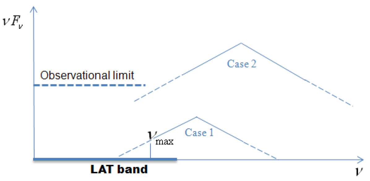
Figure 2: Two schematic possibilities allowing the SSC component to be compatible with LAT observations.

Let $\alpha$ denote the photon spectral index below $\nu_{peak}$, i.e. $N_{\nu}\propto\nu^{\alpha}$. Most GRBs are phenomenologically well fit by a Band function, and for these $\alpha\approx-1$. Defining $\zeta_{W}$ as the fraction of up-scattered flux observed in the LAT window, relative to the total up-scattered flux, the ratio between the expected flux up to $\nu_{max}$ and the sub-MeV flux, is:

$$\frac{F_{LAT}}{\nu_{m}F_{\nu,m}}=Y_{0}\zeta_{W}.$$ (36)

If $\nu_{KN}>\nu_{max}$ and if $\nu F_{\nu}$ is rising below $\nu_{KN}$ (as happens for $\alpha\approx-1$) then the total flux observed in the LAT window is dominated by $\nu_{max}$. $\zeta_{W}$ can be written as (Ando et al., 2008):

$$\zeta_{W}\approx\begin{cases}1,&\mbox{if }min[\nu_{SSC},\nu_{KN}]<\nu_{max}\\ (\frac{min[\nu_{SSC},\nu_{KN}]}{\nu_{max}})^{-\alpha-2},&\mbox{else.}\end{cases}$$ (37)

Plugging in $\nu_{KN}$ (i.e. assuming $\nu_{KN}<\nu_{SSC}$) yields:

$$\zeta_{W}=\begin{cases}1,\;\;\;\;\;\;\;\;\;\;\;\;\text{ if }180\nu_{max,1}^{-1}\Gamma_{2}^{2}(\epsilon)^{\frac{-1}{4}}k^{1/4}(1\!+\!k)^{-3/4}\nu_{p,300}^{1/4}t_{p,.3}^{1/2}F_{-26.2}^{-1/4}d_{28}^{-1/2}<1\\ (180\nu_{max,1}^{-1}\Gamma_{2}^{2}(\epsilon)^{\frac{-1}{4}}k^{1/4}(1\!+\!k)^{-3/4}\nu_{p,300}^{1/4}t_{p,.3}^{1/2}F_{-26.2}^{-1/4}d_{28}^{-1/2})^{-\alpha-2}\text{ else}\end{cases}$$ (38)

where $h\nu_{max,1}\equiv\frac{\nu_{max}}{1GeV}$.

We require that the SSC contribution will be sufficiently low to agree with the LAT observations. We separate the possible solutions to two cases.

If $\epsilon>2.4k^{-1/7}(1+k)^{3/7}\nu_{p,300}^{-5/7}t_{p,.3}^{-2/7}F_{-26.2}^{1/7}d_{28}^{2/7}\eta_{LAT-1}^{-8/7}$, then, $\frac{F_{SSC}}{\nu_{m}F_{\nu,m}}=Y_{0}<0.1\eta_{LAT-1}$ and the total up-scattered flux (and not just the fraction within the considered band) is below the observed limit. Otherwise, the total ratio of up-scattered to synchrotron flux is larger than $0.1\eta_{LAT-1}$, but it peaks at $\nu_{KN}\gg\nu_{max}$ and thus may be partially absorbed. As $\Gamma$ increases, the up-scattered flux peaks at higher frequencies. This means, that for large enough values of $\Gamma$, the up-scattered tail below $\nu_{max}$ is small enough that it is compatible with the observations. Therefore, in this regime of $\epsilon$, one can obtain a lower limit on $\Gamma$ in terms of $\eta_{LAT}$ arising from the requirement that the total up-scattered flux up to $\nu{max}$ be less than the flux observed by LAT:

$$\Gamma_{2}>10^{-\frac{2.25\alpha-4.27}{2\alpha+4}}\eta_{LAT-1}^{\frac{-1}{2\alpha+4}}\nu_{max,1}^{1/2}\epsilon^{\frac{2\alpha+1}{8(2\alpha+4)}}k^{-\frac{2\alpha+5}{8(2\alpha+4)}}(1\!+\!k)^{\frac{6\alpha+15}{8(2\alpha+4)}}\nu_{p,300}^{-\frac{2\alpha+9}{8(2\alpha+4)}}t_{p,.3}^{-\frac{2\alpha+5}{4(2\alpha+4)}}F_{-26.2}^{\frac{2\alpha+5}{8(2\alpha+4)}}.$$ (39)

Notice that these are conservative limits as we only use the spectral range below $\nu_{max}$ where we know the conditions are optically thin. One must bear in mind, that efficiency considerations limit the amount of energy that may be carried by the up-scattered flux by virtue of Eq. 41. This limits $\epsilon$ but not $\Gamma$.

3.4 Results

Figs. 3, 4 depict the different GRB parameters superimposed on the allowed space in the $(\epsilon,\Gamma)$ plane arising from the above conditions. We plot here results for $k=1$ and $k=10$. The condition that the SSC flux resides below the observational limits within the frequency range up to the maximal observed photon energy is plotted for $\nu_{max}=71$GeV (source frame) corresponding to the highest (prompt) energy photon to date, from 080916C. They are drawn for two cases of the lower spectral slope: $\alpha=-1$ and $\alpha=-1.5$. We choose to take the most extreme values for this limit, in order to show that even in this case, there is still reasonable parmeter space in the $(\epsilon,\Gamma)$ plane. We return to this extreme case in greater detail in §5.

Several characteristic features can be seen in these figures. First, $R$ is directly related to the pulse duration and bulk Lorentz factor via Eq. 2, and it is independent of $\epsilon$. For the canonical observed parameters we use here, $R$ spans two orders of magnitude, $10^{15}k^{-1/8}(k+1)^{1/24}t_{p,.3}\mbox{cm}<R<10^{17}k^{-3/8}(k+1)^{1/8}t_{p,.3}\mbox{cm}$, and it is relatively large. $B$ is the most fluctuating parameter spanning almost 4 orders of magnitude: $3k^{-5/16}(k+1)^{1/16}\nu_{p,300}^{1/2}t_{p,.3}^{-1}F_{-26.2}^{1/2}d_{28}\mbox{ Gauss}<B<10^{4}k^{1/16}(k+1)^{-3/16}\nu_{p,300}^{1/2}t_{p,.3}^{-1}F_{-26.2}^{1/2}d_{28}\mbox{ Gauss}$. The lines of constant $B$ are almost parallel to the $\nu_{m}=\nu_{c}$ line, which means that the value of $B$ is almost a direct representative of $x_{ins}$, the fraction of instantaneously emitting electrons relative to the total number of electrons. The allowed range for $\gamma_{m}$ is: $3\times 10^{3}k^{3/16}(k+1)^{-11/48}\nu_{p,300}^{1/4}t_{p,.3}^{1/2}F_{-26.2}^{-1/4}d_{28}^{-1/2}<\gamma_{m}<10^{5}k^{1/16}(k+1)^{-3/16}\nu_{p,300}^{1/4}t_{p,.3}^{1/2}F_{-26.2}^{-1/4}d_{28}^{-1/2}$. These high values of $\gamma_{m}$ (compared with $m_{p}/m_{e}$) are extremely significant for GRB models in which the electrons are heated by shocks and the initial energy resides in protons. In these cases, it is necessary that only a small fraction of electrons will be heated to relativistic velocities in order to allow them to reach such high energies (Daigne $\&$ Mochkovitch, 1998; Bošnjak et al., 2009). We show this explicitly for the internal shocks model in §4. In addition, we observe that $\nu_{KN}$ is expected to lie in the range: $250k^{1/8}(k+1)^{7/24}\nu_{p,300}^{1/4}t_{p,.3}^{1/2}F_{-26.2}^{-1/4}d_{28}^{-1/2}\mbox{GeV}<\nu_{KN}<1.7k^{-1/8}(k+1)^{3/8}\nu_{p,300}^{1/4}t_{p,.3}^{1/2}F_{-26.2}^{-1/4}d_{28}^{-1/2}\mbox{TeV}.$ Therefore, even with no knowledge of the LAT observations, we could have expected that the SSC does not peak in the GeV but typically at least two orders of magnitude above. This is a direct consequence of the large values of $\gamma_{m}$ required for this solution. $N_{e}$, is expected to lie between: $10^{50}k^{-1/8}(k+1)^{-7/24}\nu_{p,300}^{3/4}t_{p,.3}^{1/2}F_{-26.2}^{5/4}d_{28}^{5/2}<N_{e}<10^{52}k^{1/8}(k+1)^{-3/8}\nu_{p,300}^{3/4}t_{p,.3}^{1/2}F_{-26.2}^{5/4}d_{28}^{5/2}$.

Even for the highest observed photon energy of 71 GeV, we see that the lower limits on $\Gamma$ that arise from the SSC flux in the GeV are less constraining than the lower limits that arise from the optical depth. However, the SSC limits become very strong for small values of the lower spectral slope, as expected in the fast cooling synchrotron regime. For the expected $\alpha=-1.5$ (which is found for $10\%$ of the GRBs in the GBM and BATSE samples) $\epsilon\gtrsim 3\times 10^{-3}$ for $k=1$ ($\epsilon\gtrsim 2\times 10^{-2}$ for $k=10$). In addition, very negative values of $\alpha$, push solutions with relatively low $\epsilon$ towards the marginally fast solution ($\nu_{c}\approx\nu_{m}$) as discussed in §3.6. By Eq. 23, the lower limit on $\Gamma$ varies as $k^{-3/48}(1+K)^{25/48}$ and therefore increases for $k\lessgtr 1$. The upper limit that arises from $\nu_{c}<\nu_{m}$ scales as $k^{-3/16}(1+K)^{9/16}$, and also increases for $k\lessgtr 1$. similarly the allowed parameter space increases with $k\lessgtr 1$.

The main effect of increasing $k$ is to increase the allowed values for $\Gamma$. The allowed range for $\Gamma$ is roughly $150<\Gamma<3000$ for $k=1$ and $300<\Gamma<6000$ for $k=10$. This range is narrowed down by considering the pair creation opacity limits and it will be addressed again in §5. Interestingly, increasing $k$ does not change significantly other parameters of the model, $R,B,\gamma_{m},\mbox{and}N_{e}$. $R\propto\Gamma^{2}/k$ implies that the lower limit on the radius scales as $k^{-1/8}(k+1)^{1/24}$ while the upper limit scales as $k^{-3/8}(k+1)^{1/8}$. Thus, even for relatively large $k$ one expects a comparable range of emission radii to the one obtained for $k=1$. For the magnetic field, the lower limit scales as $k^{-5/16}(k+1)^{1/16}$ while the upper limit depends on $k^{1/16}(k+1)^{-3/16}$. Again, the allowed range of $B$ varies very weakly with $k$, and $3$ Gauss and $10^{4}$ Gauss are strict lower and upper limits. The range of electrons Lorentz factors varies with a lower limit $\propto k^{3/16}(k+1)^{-11/48}$, and an upper limit $\propto k^{1/16}(k+1)^{-3/16}$ yielding a strict upper limit of $\approx 10^{5}$ (obtained for $k=1$) and a weakly varying lower limit of order 3000. Finally, the lower limit on the number of electrons is $\propto k^{-1/8}(k+1)^{-7/24}$, while the upper limit is $\propto k^{1/8}(k+1)^{-3/8}$ implying a strong upper limit on the number of relativistic electrons $\approx 10^{52}$.

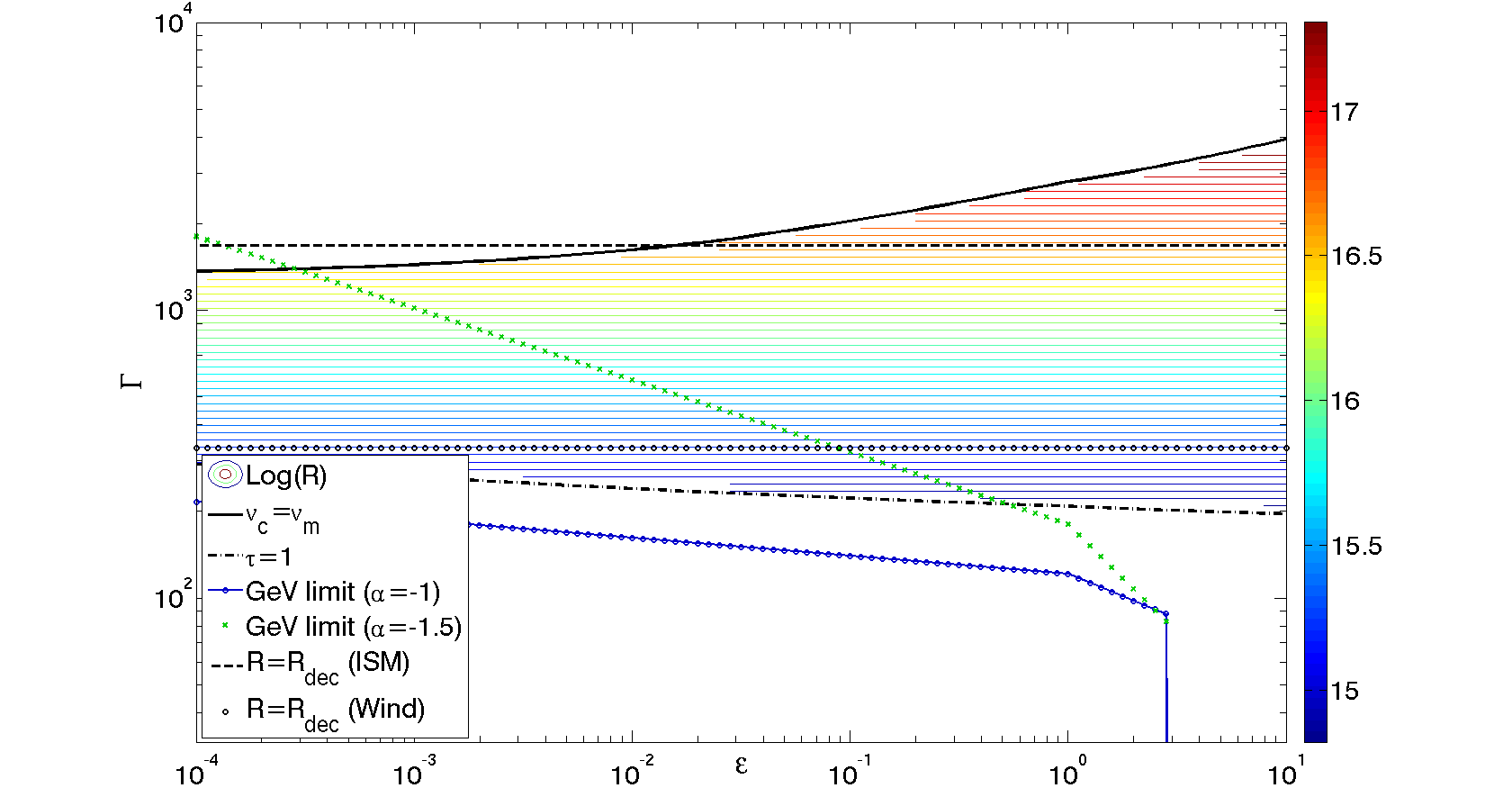
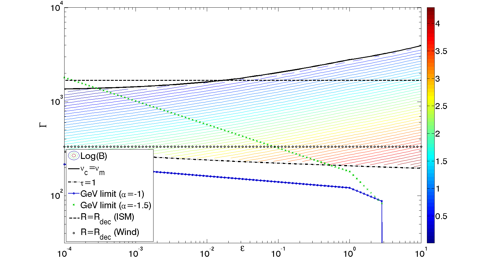
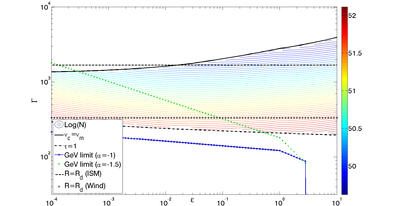
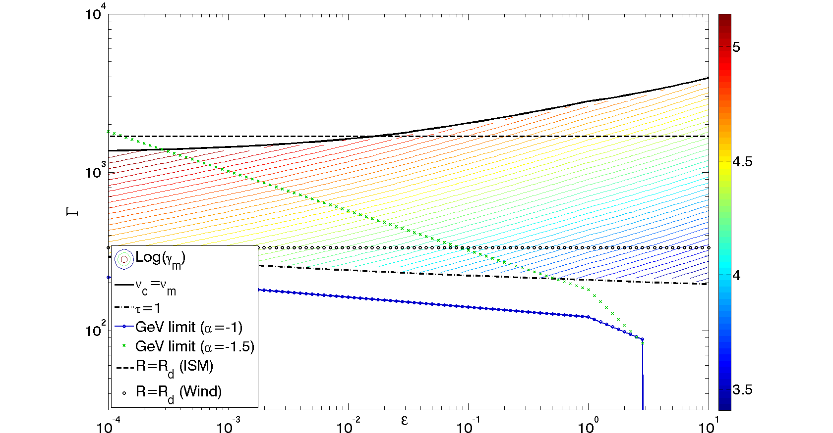
Figure 3: The range of GRB parameters for typical observables ($t_{p.3}$,$F_{-26.2}$,$d_{28}$,$\nu_{p,300}$) in the $(\epsilon,\Gamma)$ plane for $k=1$. Plotted here (from top left in clockwise order) are: $R,B,\gamma_{m},N_{e}$. Colours depict the values of these parameters. The conditions $\tau<1$ (bottom horizontal line) and $\nu_{c}<\nu_{m}$ (top curved line) impose strict limits on the parameter space. The area between them is available for Synchrotron solutions. The requirement that the SSC signal is below the observational limits in the GeV range, leads to lower limits on $\Gamma(\epsilon)$ which are depicted by the blue circles for the typical lower spectral index ($\alpha=-1$) and by green X’s for the expected slope in the fast cooling regime ($\alpha=-1.5$). The sharp cut-off in these limits corresponds to the transition between $\frac{F_{SSC}}{\nu_{m}F_{\nu,m}}=Y_{0}<0.1\eta_{LAT-1}$ where the total up-scattered flux is below the observational limit, to $\frac{F_{SSC}}{\nu_{m}F_{\nu,m}}=Y_{0}>0.1\eta_{LAT-1}$ where the up-scattered signal should peak at high enough energies so that the flux residing in the observed band is sufficiently low to account for the observations. These are cases 1 and 2 in Fig. 2 correspondingly. Two other conditions $R<R_{dec}(\mbox{Wind})$ and $R<R_{dec}(\mbox{ISM})$ impose softer limits (the areas below these lines are allowed for each case) on the possible solutions as they both depend on additional unknown parameters ($A_{*}$ and $n_{0}$).

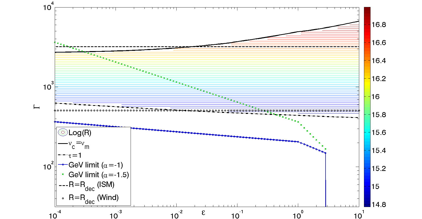
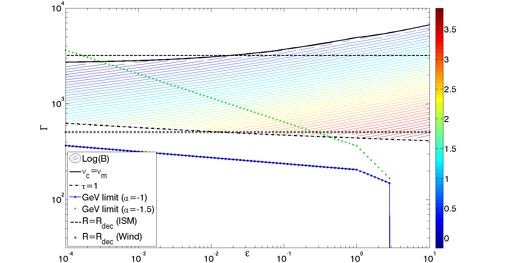
Figure 4: Same as Fig. 3 but for $k=10$.

3.5 Energetics and efficiency

We denote by $E_{int}$ the fraction of the overall energy in the flow, $E_{tot}$, that is dissipated into internal energy. In turn, part of this energy, $E_{syn}$, is radiated by synchrotron to produce the sub-MeV peak. Thus, we define:

$$E_{syn}=\eta_{syn}E_{int}=\eta_{syn}\eta_{int}E_{tot}\equiv\eta_{tot}E_{tot}.$$ (40)

$\eta_{int}$ is the conversion efficiency of bulk to internal energy in the prompt phase, i.e. the efficiency of the energy dissipation process, and $\eta_{syn}<1$ is the conversion efficiency from internal energy to radiation. GRBs must be highly efficient and must emit a significant fraction of the total kinetic energy in the sub-MeV to avoid an “energy crisis”, i.e. $\eta_{tot}$ cannot be much less than unity (Panaitescu and Kumar, 2002; Granot et al., 2006; Fan et al., 2006).

The value of $\eta_{int}$ is determined by the energy dissipation process and is therefore not the subject of this paper. We remark, however, that in many models $\eta_{int}$ is expected to be relatively low. For example, in the internal shocks model it is expected that $\eta_{int}\lesssim 0.2$ (Kobayashi et al., 1997; Daigne $\&$ Mochkovitch, 1998; Belborodov, 2000; Guetta et al., 2001). Notice, however, that an exception is possible,in case the same energy can be reprocessed to internal energy more than once leading to $\eta_{int}>1$ (Kobayashi et al., 2001). It is unknown how natural this scenario is and we leave the discussion on this possibility for future studies. We conclude that quite generally $\eta_{syn}$ must be smaller than unity.

Two efficiency criteria determine the efficiency of the synchrotron signal. First, the energy radiated by synchrotron is limited by the energy of the relativistic electrons. Therefore, we focus here on fast cooling to avoid an extra loss in the efficiency. This means that $\eta_{syn}\leqslant\epsilon_{e}$ and therefore $\epsilon_{e}$ cannot be too small. Accounting for SSC losses in addition to synchrotron losses, this translates to an upper limit on $\epsilon$. On the other hand, $\epsilon$ is also bounded from below by the requirement that SSC loses are not too large. $\frac{F_{SSC}}{\nu_{m}F_{\nu,m}}\equiv Y_{0}$ is a function of $\epsilon$, independent of the bulk Lorentz factor, but in the KN regime it may still depend on $k$ and on the various observed parameters. As seen from Eq. 30, apart for the peak frequency and pulse duration (which can span over a large range of values), all of these dependencies are very weak and have no significant effect on the overall efficiency. We examine the dependence of $\eta_{syn}$ on $\nu_{p}$ and $t_{p}$ in Fig. 5.

Figure 5: An upper limit on the efficiency when the sub-MeV peak is ascosiated with fast cooling synchrotron emission, as a function of $\epsilon$. The electrons must carry a significant amount of the energy, but too strong an amount will lead to a large amount of energy released at frequencies far above the peak by the KN process. The left panel shows the dependence on $\nu_{p}$ while the right panel shows the dependence on the pulse duration. These plots depict upper limits on the efficiency, as they do not include the efficiency of the energy dissipation process or energy losses in components other than magnetic fields or electrons.

Combining all these efficiency factors, we get the overall efficiency:

$$\eta_{tot}=\eta_{int}\eta_{syn}=\frac{\eta_{int}\epsilon_{e}}{1+Y_{0}}.$$ (41)

As $\eta_{int}$ alone is already expected to be relatively low, this limits $\eta_{syn}\gtrsim 0.1$ in order to assure that the overall efficiency satisfies: $\eta_{tot}>10^{-2}$. Thus, we must have: $10^{-4}<\epsilon<10$ (see Fig. 5). Notice that this result is independent of the bulk Lorentz factor, and it is weakly dependent on $k$ and the observed parameters. Out of these, the strongest dependence is on $\nu_{p}$. $\nu_{p}\approx 100$KeV ($\nu_{p}\approx 1000$KeV) increases (decreases) the lower limit on $\epsilon$ to about $10^{-3}$ ($10^{-5}$). Although low $\nu_{peak}$ results in low efficiencies, such bursts are usually observed with lower luminosities, and the energetic requirements for such bursts are not unreasonable. We return to this point in more detail in §3.7. The efficiency depends more weakly on the pulse duration, but the latter spans at least three orders of magnitude and thus can cause noticeable change. Taking $t_{p}\approx 5\times 10^{-2}$sec ($t_{p}\approx 5$sec) yields $\epsilon\gtrsim 3\times 10^{-4}$ ($\epsilon\gtrsim 10^{-5}$). Later on, we find that high magnetization is favored by other reasons as well.

3.6 The spectral shape

The solutions given in 3.2 consider only the peak frequency and the peak flux, disregarding the spectral shape. In the fast cooling scenario (considered here) the slope of the photons’ number spectrum above the peak of $\nu F_{\nu}$ is ($\nu^{\beta}\propto\nu^{-(p+2)/2}$) (Sari and Piran, 1997a). This is consistent with the average observed slope ($\beta=-2.3$) for $p\approx 2.6$ which is approximately the expected value for $p$ in case the electrons are accelerated by the Fermi mechanism (Achterberg et al., 2001) (Although it is not clear that the spread of $\beta$ is consistent with the expected spread in $p$ (Shen, 2006; Starling, 2008; Curran, 2010)). However, the synchrotron fast cooling slope below the peak of $\nu F_{\nu}$ ($\nu^{\alpha}\propto\nu^{-1.5}$) (Cohen et al., 1997; Sari et al., 1998; Ghisellini et al., 2000), is inconsistent with the average observed slope $\alpha=-1$ and $90\%$ of bursts have steeper slopes than this (Preece et al., 2000; Ghirlanda et al., 2002; Kaneko, 2006; Nava et al., 2011). Furthermore, the lower energy slope in about $40\%$ of GRBs is $\alpha>-2/3$ (Nava et al., 2011) which is impossible in a synchrotron scenario, even in the case of slow cooling. This is known as the synchrotron “line of death” (Preece et al., 1998). An extra concern, is that the break observed at $\nu_{peak}$ is often too sharp to be compatible with the smooth transition expected from the synchrotron model (Pelaez et al., 1994).

The synchrotron “fast cooling - line of death” problem, the more serious of the two, can be partially resolved if the electrons are marginally fast cooling (Daigne et al., 2011) with $\nu_{m}\approx\nu_{c}$. This requires, of course, an additional fine tuning mechanism that keeps this condition satisfied. To examine the possible parameter phase space with a “marginal fast cooling” we define a marginally fast solution as one that obeys one of two criteria. Either it is a fast cooling solution ($\nu_{m}>\nu_{c}$) that obeys: $\nu_{m}<3\nu_{c}$ (If $\nu_{m}$ were much larger, there would be a large range of frequencies where $\alpha=-1.5$ and the “fast cooling - line of death” problem would not be solved); or it is a a slow cooling solution ($\nu_{c}>\nu_{m}$) (where $\alpha=-2/3$ is always valid so long as we associate $\nu_{m}$, and not $\nu_{c}$, with the observed sub-MeV peak) which is sufficiently efficient, with: $\eta_{syn}>0.1$. This family of solutions, is seen in Fig. 6 and it occupies a significant area in the parameter space. The break in the slopes of the parameters in the ($\Gamma,\epsilon$) plane is due to the switch from the fast to slow cooling regime. The upper curve is the limit on the marginally fast solution due to efficiency. These lines cross the $\nu_{c}=\nu_{m}$ line at $\epsilon\approx 10^{-4}$ and $\epsilon\approx 10$ which is where the fast cooling efficiency falls below 0.1 (see Fig. 5). The marginally-fast solutions are characterized by $t_{c}(\gamma_{m})\approx t_{p}$, and therefore $x_{int}\approx 1$ and the instantaneous number of emitting electrons is about the same as the total number of relativistic electrons. The allowed region has high values of $\Gamma$ and $\gamma_{m}$: $\Gamma\gtrsim 700$, $\gamma_{m}\approx 10^{5}$, relatively small values of $N_{e}$: $N_{e}\approx 10^{50}$, a weak (and almost constant) magnetic field: $B\approx 10\mbox{ Gauss}$ and a large emission radius $R\gtrsim 3\times 10^{16}cm$. A canonical wind solution is ruled out for these solutions. Another partial solution to the “line of death” problem, can be achieved in case SSC occurs in the KN regime, as was shown in §3.3 to be the generic case. In such cases, detailed modeling, shows that $\alpha$ can be increased from -1.5 to -1 (Derishev, 2003; Nakar et al., 2009; Wang, 2009; Daigne et al., 2011; Barniol Duran et al., 2012). However, this solution requires very low values of $\epsilon$ and with $\epsilon\gtrsim 10^{-4}$, as required by efficiency considerations (see §3.5), one is still limited to $\alpha<-1.2$.

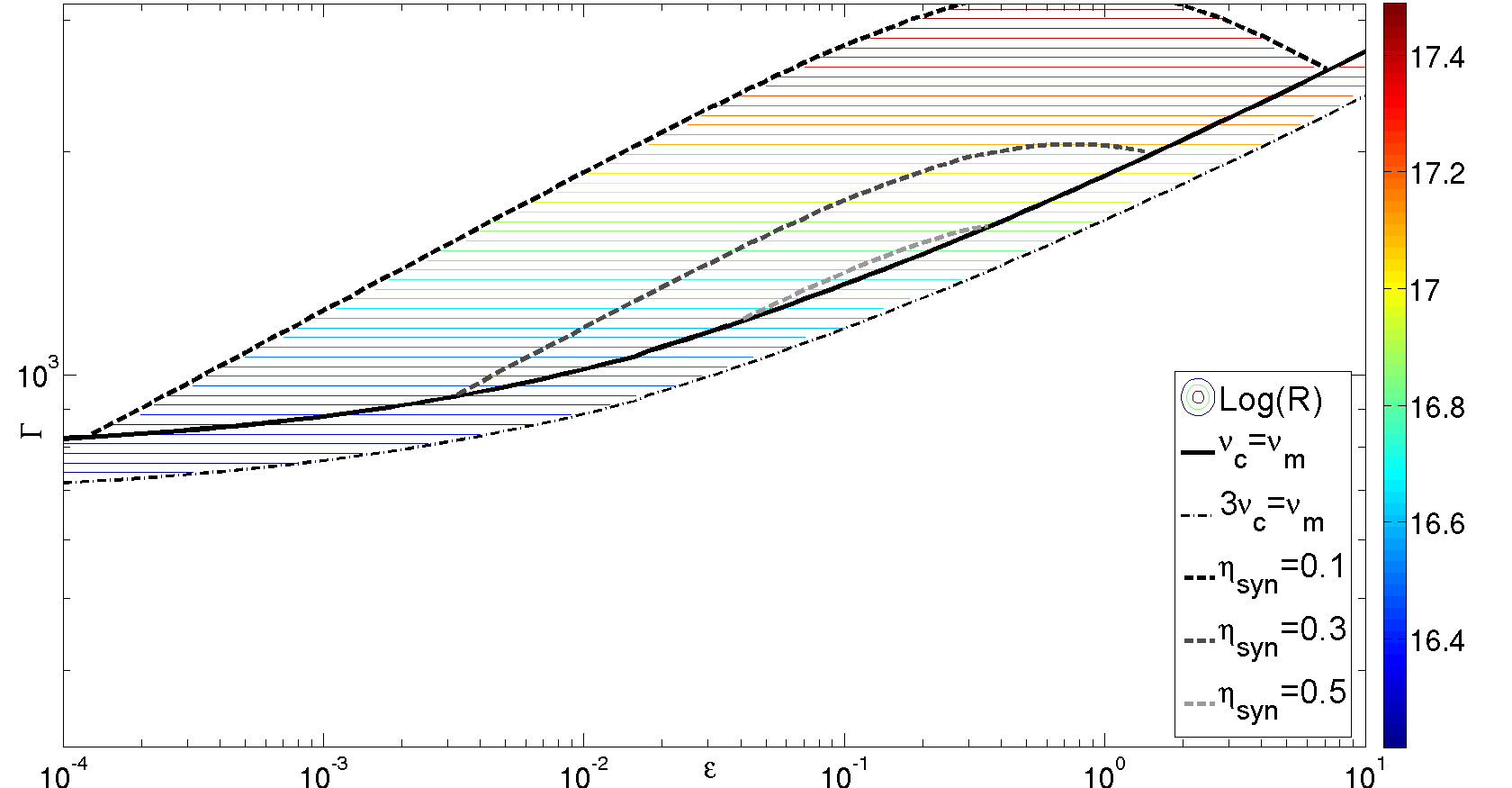
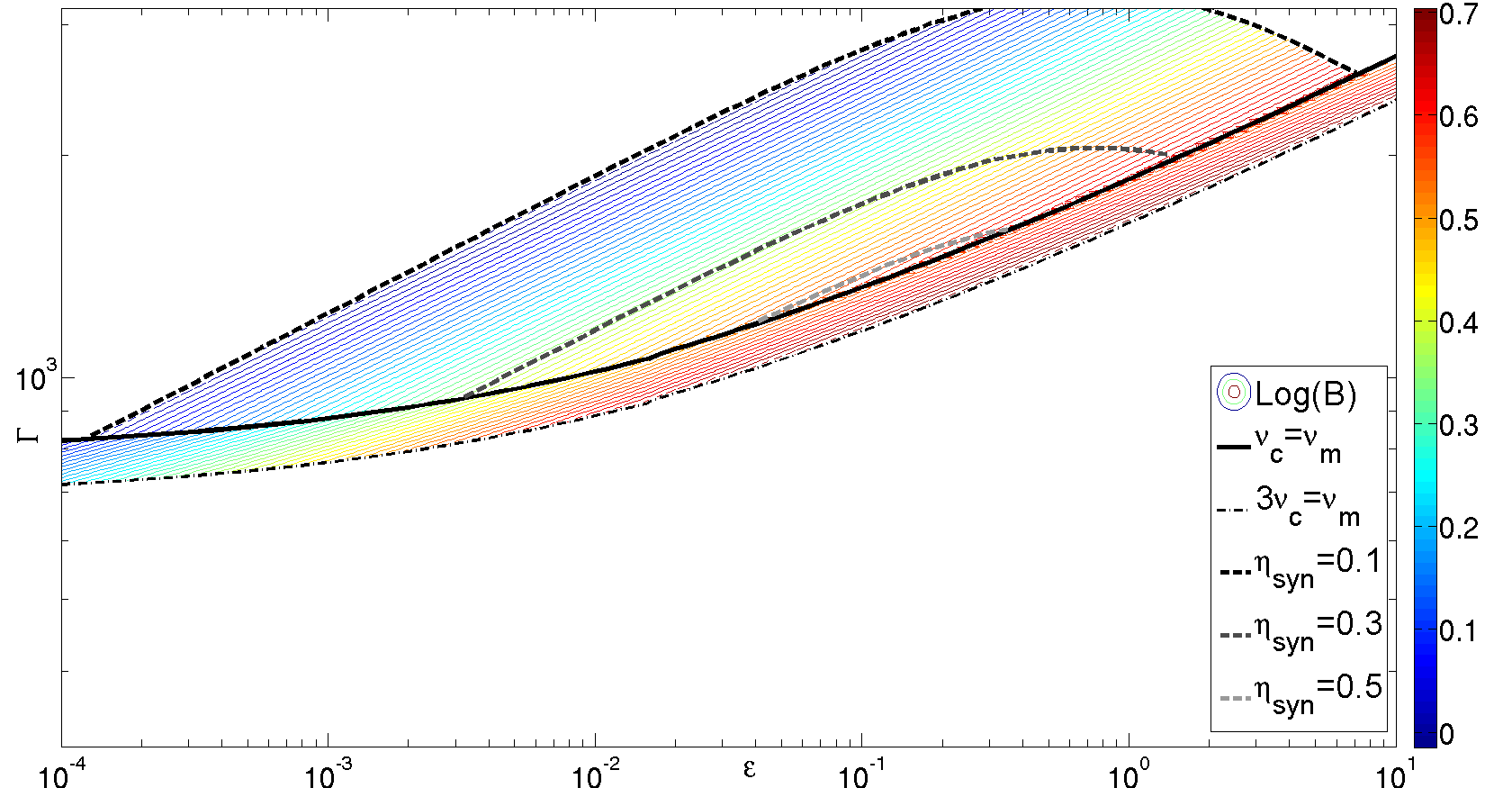
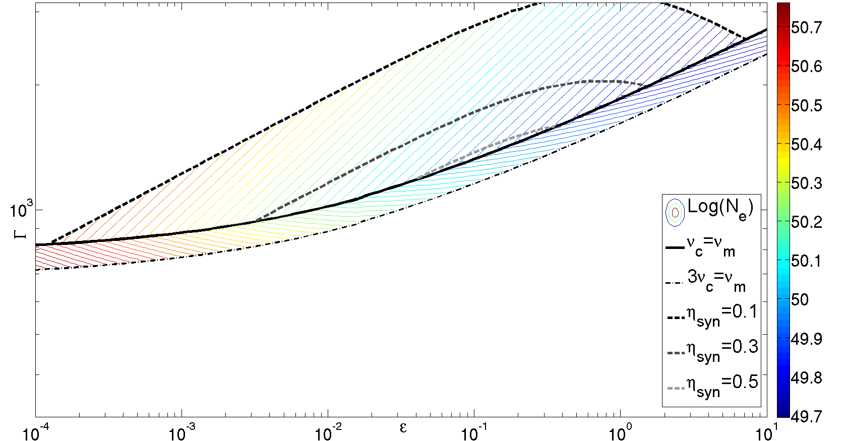
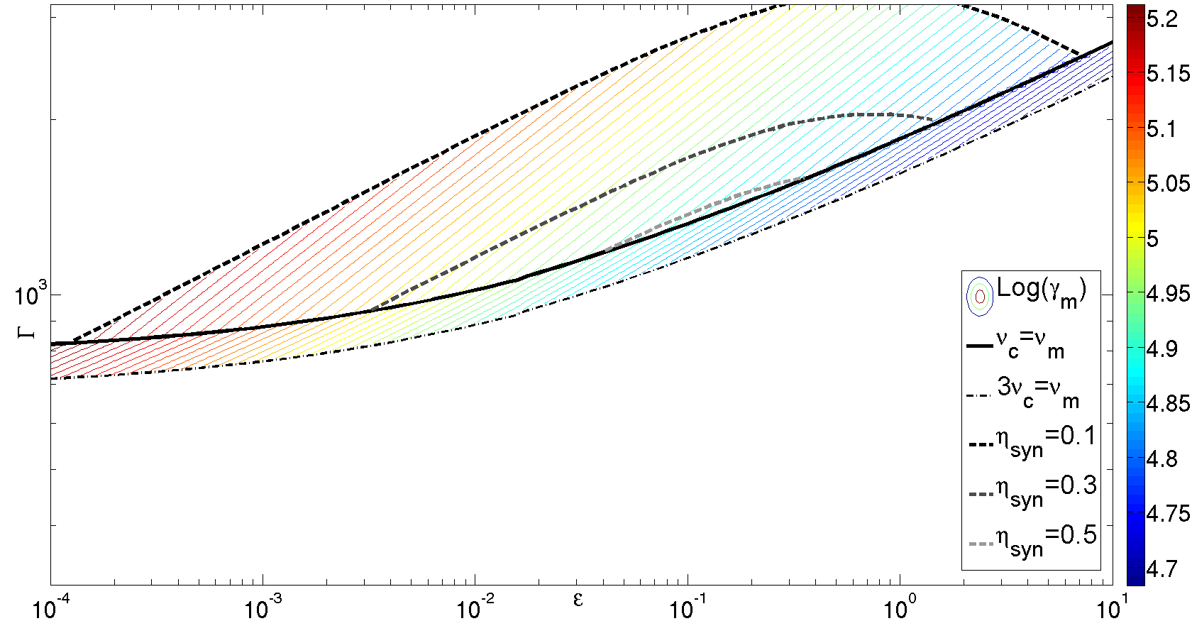
Figure 6: The range of GRB parameters for a marginally fast solution in the $(\epsilon,\Gamma)$ plane for $k=1$, $\xi=1$. Plotted here (from top left in clockwise order) are: $R,B,\gamma_{m},N_{e}$. Below the dashed line ($\nu_{m}=3\nu_{c}$) there is a sufficiently large frequency range between $\nu_{c}$ and $\nu_{m}$ leading to $\alpha=-1.5$ below the sub-MeV peak which is incompatible with the marginally fast solution. Above the black dot-dashed line, the radiative efficiency falls below 0.1. In addition are plotted the lines of $\eta_{syn}=0.5,0.3$ in grey dot-dashed lines.

A complete solution to the “line of death” problem within synchrotron emission can be achieved if the synchrotron self absorption frequency, $\nu_{SSA}$, is sufficiently close to $\nu_{m}$. Extrapolating the fast cooling synchrotron flux below $\nu_{m}$ and equating it to the black body limit (Granot et al., 2000) we can estimate $\nu_{SSA}$:

$$\frac{2\nu_{SSA}^{2}}{c^{2}}\gamma(\nu_{SSA})\Gamma m_{e}c^{2}\frac{R^{2}}{4\Gamma^{2}d_{L}^{2}}=F_{\nu,max}(\nu_{SSA}/\nu_{m})^{-1/2}$$ (42)

where $\gamma(\nu_{SSA})$ is the typical thermal Lorentz factor of electrons radiating at $\nu_{SSA}$. Eq. 42 yields a (source frame) self absorption frequency of:

$$\frac{\nu_{SSA}}{\nu_{p,300}}=9.2\times 10^{-5}(1+Y_{0})^{1/12}\Gamma_{2}^{-4/3}(\epsilon)^{1/12}k^{-1/12}(k+1)^{11/12}\nu_{p,300}^{-3/4}t_{p,.3}^{-5/6}F_{-26.2}^{5/12}d_{28}^{5/6}.$$ (43)

Typically, $\nu_{SSA}$ is about 4 orders of magnitude bellow $\nu_{p}$ and it depends weakly on the various parameters. It is therefore, unlikely that self absorption has any significant effect on $\alpha$.

A final possibility that should be mentioned in the “line of death” context is that $\alpha$ may be affected by the presence of a sub-dominant thermal component which is expected to occur in the fireball model at a level of a few percent of the total prompt energy (Mészáros $\&$ Rees, 2000; Daigne $\&$ Mochkovitch, 2002; Nakar et al., 2005). Detailed spectral modeling, shows that adding a weak sub-dominant thermal component usually causes $\alpha$ to decrease (Guiriec et al., 2011, 2012).

3.7 The Distribution of $E_{peak}\backslash L_{peak}$

There have been many claims that the distribution of $E_{peak}$ is rather narrow (Band, 1993; Mallozzi et al., 1995; Brainerd et al., 1999; Schaefer, 2003) . Typically $E_{peak}$ values are in the range $150\mbox{ KeV}<E_{peak}<700$ KeV (Kaneko, 2006). It is not obvious that this observation reflects the intrinsic properties of GRBs and is not caused by some selection effect (Shahmoradi, 2010). Softer bursts have been detected by Beppo-SAX and HETE2, and Fermi is finding much higher $E_{peak}$ bursts. However, if true, this result is surprising in the general framework of the Synchrotron model, where one expects $E_{peak}=h\nu_{m}\propto\Gamma\gamma_{m}^{2}B$ and it is not obvious why this specific combination of parameters will remain fairly constant between different pulses and different bursts. Furthermore, there have been claims that $E_{peak}$ may be correlated with the peak luminosity, $L_{peak}$, (Yonetoku et al., 2010) and that therefore the distributions of both are not statistically independent.

To examine this issue we examine four characteristic bursts in the $(E_{peak},L_{peak}$) plane:

1. Low $E_{peak}$ ($100KeV$) and low $L_{peak}$ ($3\times 10^{51}erg/sec$) (low end of Yonetou relation).

2. High $E_{peak}$ ($1000KeV$) and high $L_{peak}$ ($1.5\times 10^{53}erg/sec$) (high end of Yonetoku relation).

3. High $E_{peak}$ ($1000KeV$) and low $L_{peak}$ ($3\times 10^{51}erg/sec$) (“above” the Yonetoku relation). None of the bursts with known redshift belong to this category, but this may be an observational effect (Nakar and Piran, 2005; Band, 2005).

4. Low $E_{peak}$ ($100KeV$) and high $L_{peak}$ ($1.5\times 10^{53}erg/sec$) (“below” the Yonetoku relation). Such bursts would be relatively easier to detect (many photons) but are not seen in observations. It is therefore believed that they do not exist.

We are interested in the range of parameters ascosiated with synchrotron solutions for these bursts. We note that $L_{peak}\propto F_{\nu_{peak}}\nu_{peak}d^{2}$, so that there is generally more than one way to realize a specific value of $L_{peak}$ with the different observed parameters. In the following discussion, we choose to take $d$ to be constant and vary $F_{\nu_{peak}}$. In terms of the allowed ranges for the synchrotron parameters we do not find any significant difference between the four typical bursts (see Fig. 7 for an example of $\gamma_{m}$ in each of these bursts). The main difference is a slight change in the limits of the allowed region corresponding to $\nu_{c}=\nu_{m}$ and $\tau=1$. This can also be seen in Fig. 8 where we plot those limits in the ($\epsilon$, $\nu_{peak}$) plane assuming that $\nu_{peak}$ and $L_{peak}$ follow the Yonetoku relation.

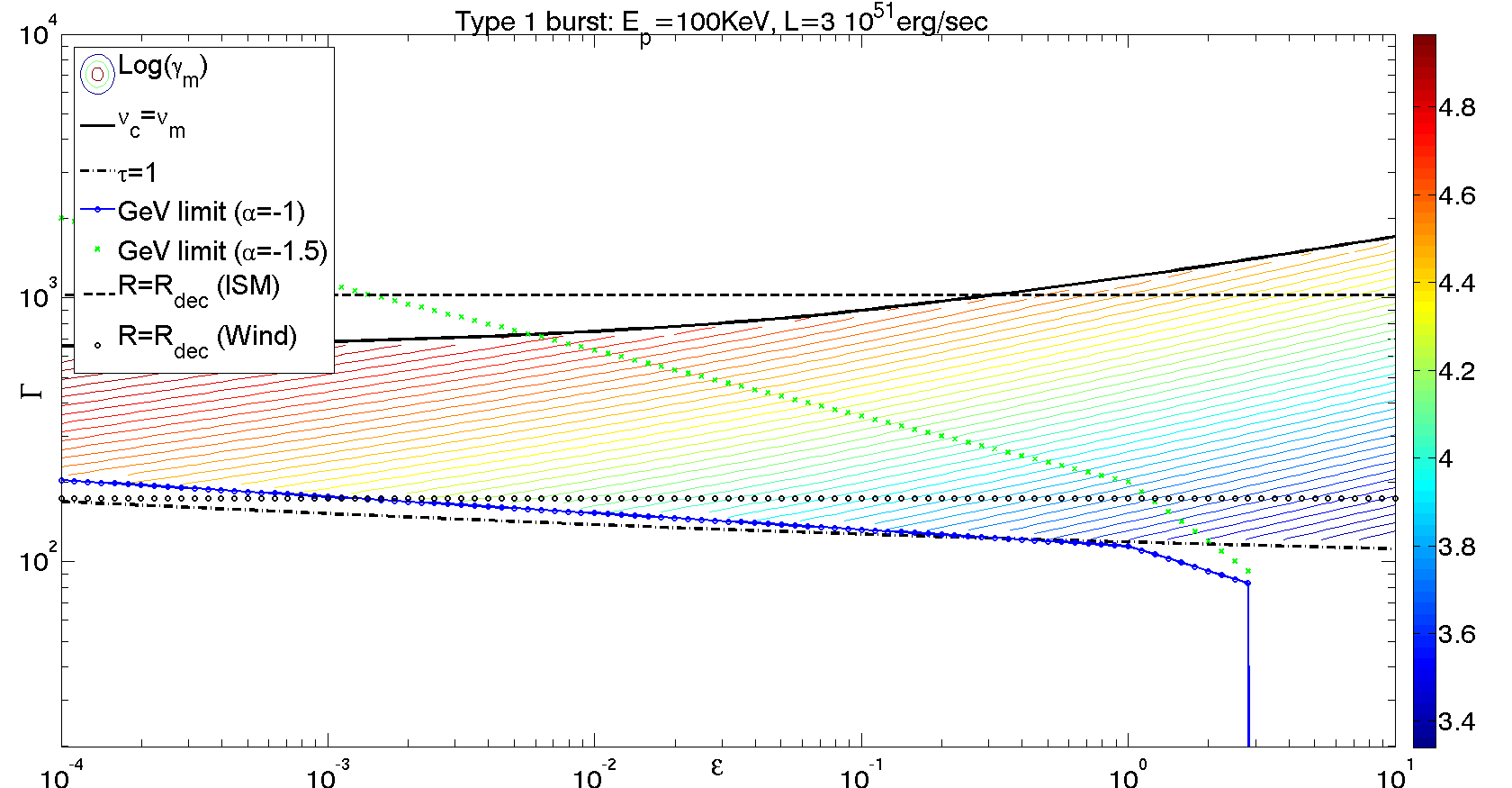
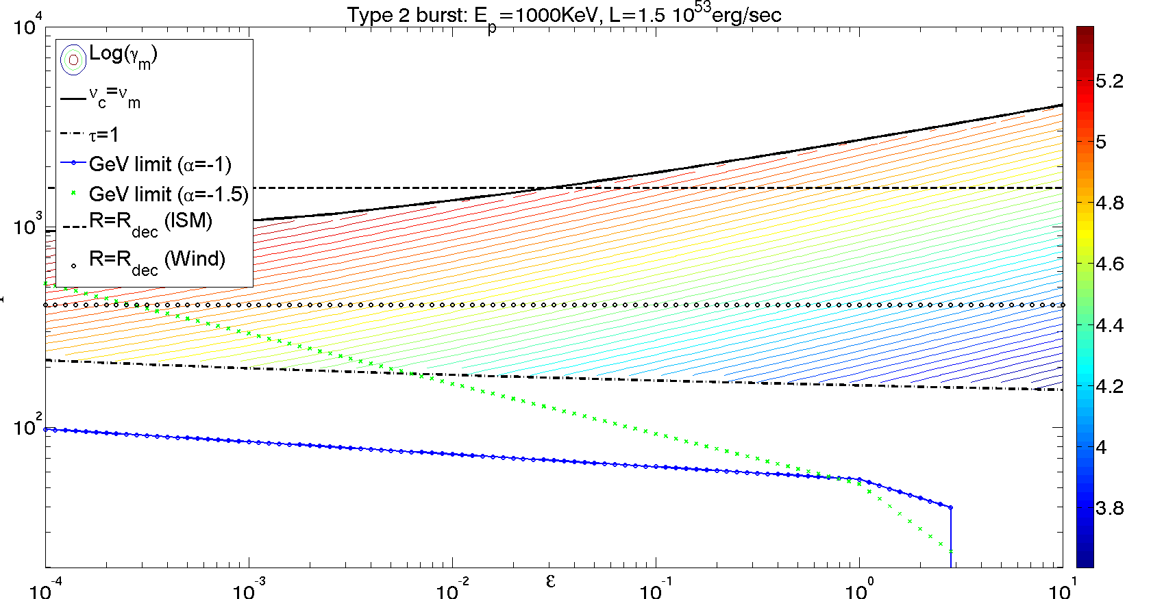
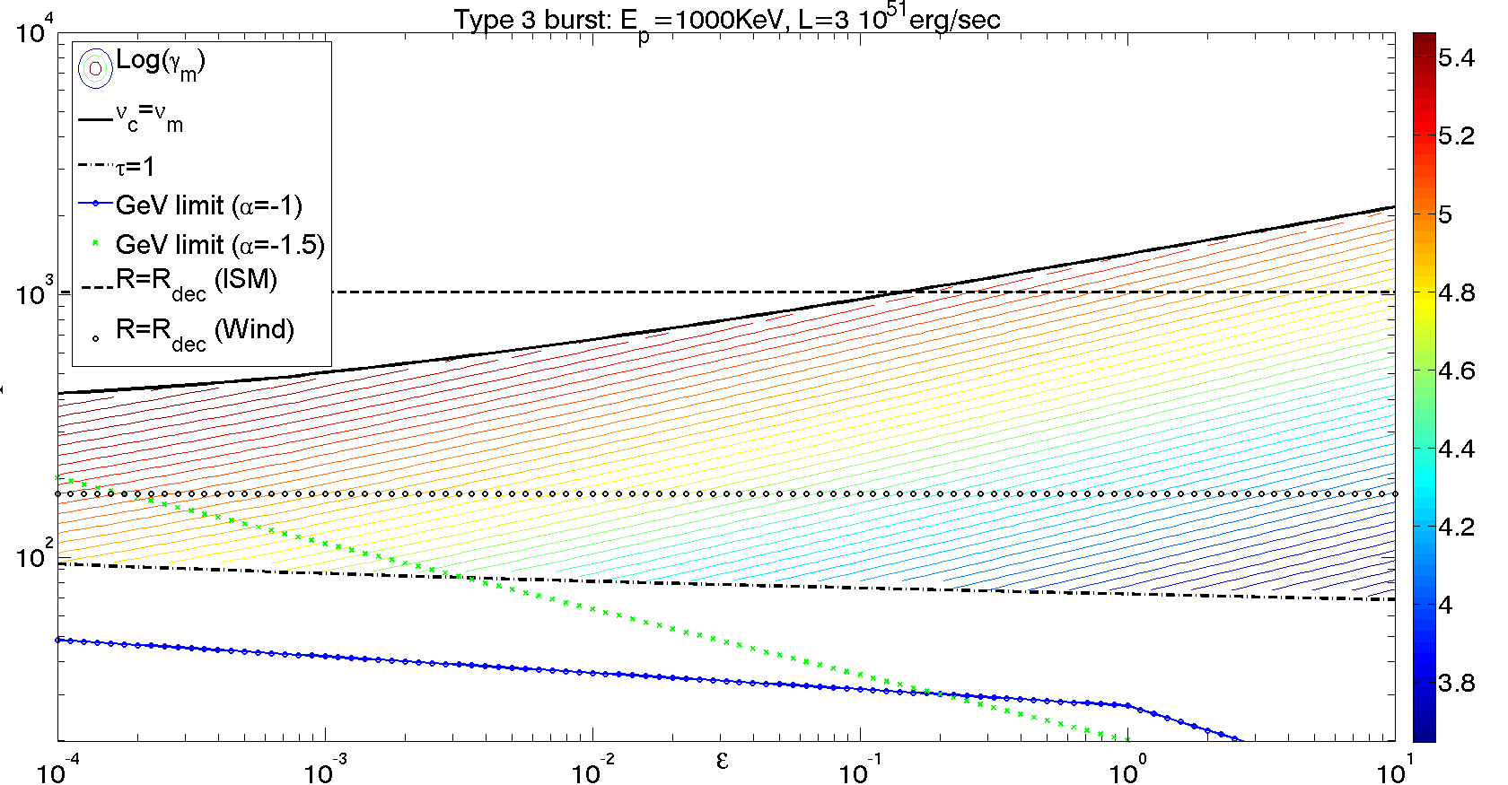
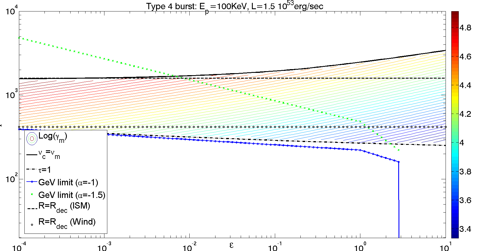
Figure 7: The range of $\gamma_{m}$ (shown by different colours) for four types of bursts in the $(\epsilon,\Gamma)$ plane for $k=1$, $\xi=1$. The conditions $\tau<1$ (bottom horizontal line) and $\nu_{c}<\nu_{m}$ (top curved line) impose strict limits on the parameter space. The area between them is available for Synchrotron solutions. The requirement that the SSC signal is below the observational limits in the GeV range, leads to lower limits on $\Gamma(\epsilon)$ which are depicted by the blue circles for the typical lower spectral index ($\alpha=-1$) and by green X’s for the expected slope in the fast cooling regime ($\alpha=-1.5$). Two other conditions $R<R_{dec}(\mbox{Wind})$ and $R<R_{dec}(\mbox{ISM})$ impose softer limits (the areas below these lines are allowed for each case) on the possible solutions.

In Fig. 9 we plot the radiative efficiency and minimal luminosity requirements of these bursts (as described in §3.5). A type-4 burst is the most inefficient and has the largest intrinsic power. Its synchrotron efficiency peaks at less than 0.4, and it could very likely be less, depending on the value of $\epsilon$, while its intrinsic power is at least $4\times 10^{53}erg/sec$. This may pose an explanation as to why practically no soft - high luminosity bursts are seen (i.e. bursts below the Yonetoku relation). The energetic demands for such bursts are simply too high. The other class of Yonetoku relation violators, are type 3 bursts. For these, efficiency is high and they cannot be ruled out by the same argument. However such bursts (hard and weak) have only a small number of photons (Nakar and Piran, 2005; Band, 2005) and are observationally hard to detect. This might cause fewer bursts of this kind to have a detectable redshift, leading to a natural selection effect.

Figure 8: Limits on the allowed parameter space due to $\nu_{m}\geqslant\nu_{c}$ and $\tau\leq 1$ in the ($\epsilon$, $\nu_{peak}$,$\Gamma$) space assuming that $\nu_{peak}$ and $L_{peak}$ follow the Yonetoku relation (Yonetoku et al., 2010). Fast cooling optically thin synchrotron solution an arise in the area between the two surfaces.

Figure 9: The maximal radiative efficiency of the four different types of bursts. Soft, high luminosity bursts are the least efficient and require huge energies at the source. This may explain the lack of such bursts.

Unless, typical bursts have very low $\epsilon$, the observed luminosity is much more important than $\nu_{peak}$ in order to determine the intrinsic power. Therefore, it is possible to produce bursts with low $L_{peak}$ and $\nu_{peak}$ and we conclude that this model does not naturally predict the claimed narrow distribution of $\nu_{peak}$ by efficiency arguments alone. As mentioned above, this may actually be considered as an advantage of the synchrotron model, as it is quite likely that the true peak distribution is not as narrow as previously thought. In this case, the argument would be reversed. Synchrotron would be a very natural way to produce such large peak dispersion.

4 A synchrotron solution within the internal shocks model

We divert here from the main theme of the paper, in which we consider a “model independent synchrotron emission” and examine specific additional constraints that arise when considering a situation when the energy is stored in the bulk kinetic energy of the flow. This is the case in the common internal shocks model, but is also the case in a Poynting flux dominated model if the magnetic energy has been converted to kinetic energy before the radiation process begun.

The kinetic energy of the initial flow is dominated by protons . Denoting the number of protons by $N_{p}$, we have: $N_{p}=N_{tot}$ ($2N_{e+}=N_{tot}$ for a pair dominated plasma). The total (bulk+internal) energy needed to produce a combined shell traveling with a bulk Lorentz factor $\Gamma$, in this scenario, is:

$$E_{tot}\approx g\Gamma N_{tot}m_{p}c^{2}(\times\frac{m_{e}}{m_{p}}\mbox{for pairs})$$ (44)

where the factor of $g\approx few$ arises from the fact that the colliding shells must initially have different bulk Lorentz factors in order for internal shocks to occur (the actual number depends on the amount of variations in the bulk Lorentz factor along the flow). The minimal value of $g$ (the most efficient) arises when all the initial energy is transformed into two channels: internal energy of the electrons and energy in magnetic fields. In this case $g=1/(1-\eta_{int})$. However, if some of the energy remains in thermal energy of the the protons, $g$ would be somewhat larger.

Eq. 44 yields the energy of the emitting electrons: $E_{e}=\epsilon_{e}E_{int}=\epsilon_{e}\eta_{int}E_{tot}$ in terms of the initial energy stored in the protons (or pairs). At the same time the synchrotron conditions determine the number of emitting electrons, $N_{e}$ and their Lorentz factor, $\gamma_{m}$ and this determines, in turn, the energy of the emitting electrons via Eq. 5. Comparing the two expressions we find that the number of emitting electrons is significantly lower than the total number of electrons. We define $\xi$ as the fraction of the synchrotron emitting electrons in the flow: $\xi\equiv N_{e}/N_{tot}$. A schematic picture of the electron number distribution is given in Fig. 10.

$$E_{e}=N_{e}\frac{p-1}{p-2}\Gamma\gamma_{m}m_{e}c^{2}=\xi N_{tot}\frac{p-1}{p-2}\Gamma\gamma_{m}m_{e}c^{2}$$ (45)

Using Eqns. 17, 19, 44, 45, $E_{e}=\epsilon_{e}E_{int}=\epsilon_{e}\eta_{int}E_{tot}$ becomes:

$$\xi(\Gamma,\epsilon_{B},\epsilon_{e})=\frac{N_{e}}{N_{tot}}=0.19\frac{p-2}{p-1}\frac{g}{2}\frac{\eta_{int}}{0.2}(1+Y_{0})^{1/4}\Gamma_{2}^{-1}\epsilon^{\frac{1}{4}}\epsilon_{e}k^{-\frac{1}{4}}(1\!+\!k)^{\frac{3}{4}}\nu_{p,500}^{-\frac{1}{4}}t_{p,.3}^{-\frac{1}{2}}F_{-26.2}^{\frac{1}{4}}(\times\frac{m_{e}}{m_{p}}\mbox{for pairs}).$$ (46)

The reason for these low fractions of emitting electrons is clear. The synchrotron solution requires relatively large electron Lorentz factors, of order $3\times 10^{3}<\gamma_{m}<10^{5}$. On the other hand if the available energy $\epsilon_{e}\eta_{int}E_{tot}$ is distributed to all the electrons (whose number is dictated by the initial number of protons) than the typical Lorentz factor would be of order $g\epsilon_{e}\eta_{int}(p-2)/(p-1)(m_{p}/m_{e})$ (or $g\epsilon_{e}\eta_{int}(p-2)/(p-1)$ for a pair-dominated flow). Unless g is unreasonably large, this Lorentz factors is too small by several orders of magnitude. To overcome this problem we must conclude, following Daigne $\&$ Mochkovitch (1998); Bošnjak et al. (2009) that within the internal shocks model only a small fraction of the electrons are accelerated in the shocks. It should be noted, that the conditions needed for this solution, are very different than the situation achieved in recent PIC simulations. This is because, in order for the solution presented here to work there must be a gap between the Lorentz factor of the thermal (i.e. non synchrotron emitting) electrons and $\gamma_{m}$ as depicted in Fig. 10. The ratio of the number of emitting electrons to the total number is plotted in Fig. 4 (Fig. 11 for pairs), for the limiting case of $\epsilon_{B}+\epsilon_{e}=1$ which provides an upper limit on the actual value of $\xi(\Gamma,\epsilon_{B},\epsilon_{e})$. Large values of $\Gamma$ lead to $\xi(\Gamma,\epsilon_{B},\epsilon_{e})\ll 1$. For $\Gamma>100$ (as found in §3.2), $\xi\lesssim 4\times 10^{-2}$ ($\approx 2\times 10^{-5}$ for pairs).

In case $\xi$ is very small, there are many “passive” electrons in the flow which may dominate the optical depth. $\xi_{*}$ is defined such that for $\xi<\xi_{*}$ the passive electrons dominate the total number of electrons:

$$\xi_{*}=1.4\times 10^{-3}(1+Y_{0})^{5/9}(\epsilon)^{3/8}k^{1/8}(1\!+\!k)^{-3/8}\nu_{p,300}^{5/8}t_{p,.3}^{1/4}F_{-26.2}^{-1/8}d_{28}^{-1/4}.$$ (47)

In this regime:

$$\tau=1.1\times 10^{-2}(1+Y_{0})^{5/24}\Gamma_{2}^{-6}(\epsilon)^{1/4}k^{-1/4}(1\!+\!k)^{11/4}\xi^{-1}\nu_{p,300}^{3/4}t_{p,.3}^{-3/2}F_{-26.2}^{5/4}d_{28}^{5/2}.$$ (48)

Figure 10: The electron distribution is composed of three ingredients: the power-law distributed electrons, emitting synchrotron at the sub-MeV peak, the thermal “passive” electrons which are not accelerated to high Lorentz factors and the pairs created by annihilation of high energy photons (these too, are not energetic enough to contribute to the sub-MeV spectrum). Depending on $\xi$, either the second or the third components dominate the total number.

$Log[\xi(\Gamma,\epsilon_{B},\epsilon_{e})]$ of a proton dominated flow within the internal shocks scenario The results are plotted for $g=2$, $\eta_{int}=0.2$, $p=2.5$ and $\epsilon_{B}+\epsilon_{e}=1$. This is an upper limit on the actual value of $Log(\xi)$ for real values of $\epsilon_{B},\epsilon_{e}$. Even for modest values of $\Gamma$, $\xi\ll 1$ which corresponds to a small fraction of relativistic electrons in the emitting region.

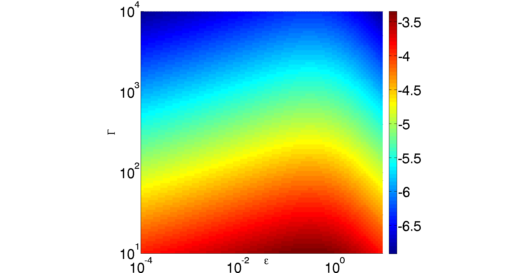
Figure 11: Same as Fig.4 but for a pair dominated flow, i.e. $Log[\xi[\Gamma,\epsilon_{B},\epsilon_{e})]$ for $g=2$, $\eta_{int}=0.2$, $p=2.5$ and $\epsilon_{B}+\epsilon_{e}=1$. For reasonable values of $\Gamma$, $\xi\lesssim 2\times 10^{-5}$.

5 pair creation opacity limit (photons above $\nu_{max}$)

The limit $\tau_{\gamma,\gamma}(\nu_{max})\leqslant 1$ leads to a lower limit on $\Gamma$ (Woods and Loeb, 1995; Piran, 1999; Lithwick $\&$ Sari, 2001). Eq. 23 shows that in the typical case, most of the electrons in the flow are not emitting the synchrotron signal, but are produced by pair creation. Therefore, the limit on $\Gamma$ from the requirement $\tau_{\gamma,\gamma}(\nu_{max})\leqslant 1$ is always more constraining than that given by Eq. 23. In order to find $\tau_{\gamma,\gamma}(\nu_{max})$ we calculate $n_{>max,an}$, the number of photons in the source with enough energy to annihilate the highest frequency photon, $\nu_{max}$ by integrating over the spectrum. This yields a lower limit on $\Gamma$:

$$\Gamma_{2}>(10^{-(4.6+1.8\beta)}|1+\beta|\nu_{max,1}^{\frac{1}{1+\beta}}(1\!+\!k)^{-2}\nu_{p,300}^{\frac{1}{1+\beta}}t_{p,.3}F_{-26.2}^{-1}d_{28}^{-2})^{\frac{2\beta-2}{(1+\beta)^{2}}}.$$ (49)

This limit is independent of $\epsilon$.

These lower limits on $\Gamma$ replace those used in Figs. 3, 4 in case the high energy photons originate from the same site as the sub-MeV emission. $\Gamma\gtrsim 300$ is required for typical parameters, a factor of two larger than the lower limit imposed by considering the optical depth for scattering of synchrotron photons. Fig. 12 depicts the allowed region in the ($\epsilon,\Gamma$) plane, arising from the lower limit on $\Gamma$ discussed here and the upper limits given by Eqns. 21, 22. The results are plotted for the most constraining GRB to date, GRB 080916C, for which $h\nu_{max}=71GeV$ (source frame) was observed. For this burst, we find very high values of the Lorentz factors: $10^{3}<\Gamma<10^{4}$, $10^{4}<\gamma_{m}<3\times 10^{5}$, and a large emitting radius $4\times 10^{16}\mbox{cm}<R<3\times 10^{18}\mbox{cm}$ that is only marginally compatible with the canonical wind parameter. Even for this extreme case, the synchrotron solution is possible. In fact, the allowed parameter space may be even larger in case the high energy emission originates from a different zone than the sub-MeV radiation (Zou et al., 2009, 2011; Hascoët et al., 2012).

As mentioned earlier, given that no opacity break is seen in the spectrum up to $\nu_{max}$, the frequency in which the system becomes optically thick to pair creation, $\nu_{thick}$ obeys: $\nu_{thick}>\nu_{max}$. So far, we still have a large uncertainty in the actual value of $\nu_{thick}$. In what follows, we argue that this uncertainty can be reduced. The higher $\nu_{thick}$ lies within the range [$\nu_{max}$,300GeV] (300GeV is the upper limit of the LAT detector), the implications of the low LAT detection rate becomes more constraining on the SSC peak (it should either peak at higher frequencies or be weak enough to account for observations). We therefore plot the combination of this pair creation opacity limit and the limit from the SSC flux in the GeV (discussed in §3.3), in Fig. 13 for $k=1$ and $k=10$. These lower limits on $\Gamma$ are more constraining for lower values of $\alpha$ (causing a smaller loss by extrapolation of the SSC from its peak to the GeV) or for low values of $\epsilon$ for which the SSC flux is larger. Quantitatively, this is described by Eq. 39. We see that in case $\nu_{thick}$ lies at the highest frequency observed by LAT (or above) and $\alpha=-1.5$, the SSC limits rule out $\epsilon\lesssim 5\times 10^{-3}$ for $k=1$ ($\epsilon\lesssim 5\times 10^{-2}$ for $k=10$).

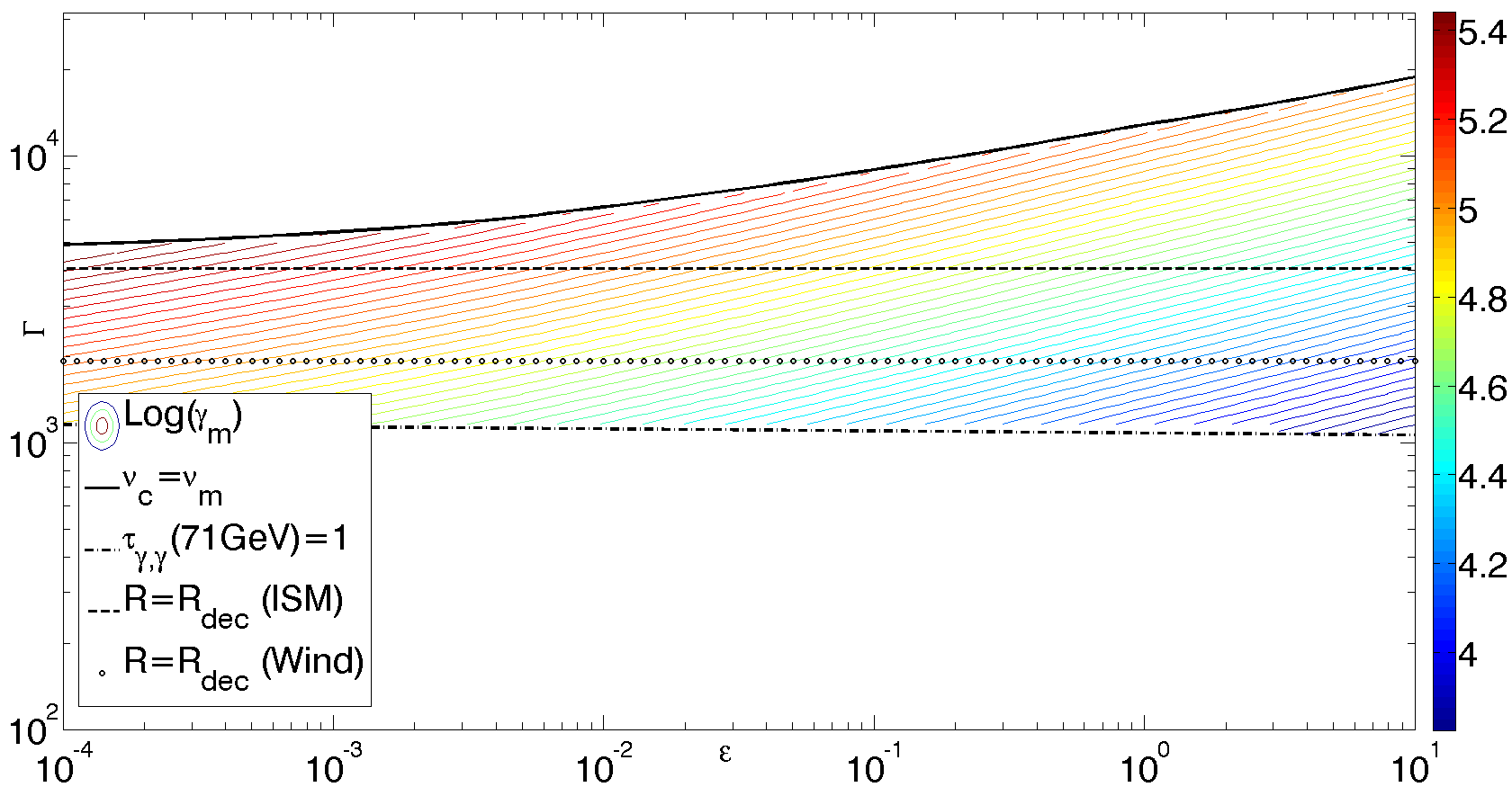
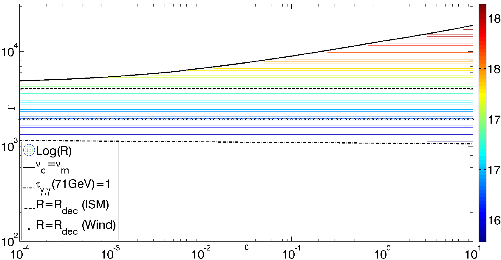
Figure 12: The allowed region in the $(\epsilon,\Gamma)$ plane for GRB 080916C, with $k=1$, $\xi=1$, $h\nu_{max}=71GeV$ (source frame). Plotted are: $\gamma_{m}$ (left panel) and $R$ (right panel). Colours depict the strength of these parameters. The conditions $\tau_{\gamma,\gamma}<1$ (bottom horizontal line) and $\nu_{c}<\nu_{m}$ (top curved line) impose strict limits on the parameter space. The area between them is available for Synchrotron solutions. Two other conditions: $R<R_{dec}(\mbox{Wind})$ and $R<R_{dec}(\mbox{ISM})$ impose softer limits (the areas below these lines are allowed for each case) on the possible solutions.

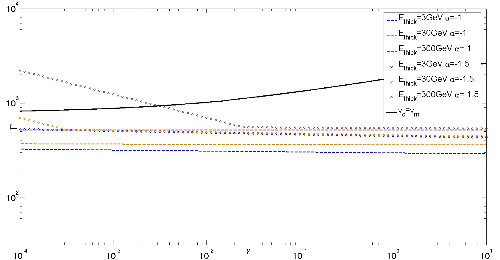
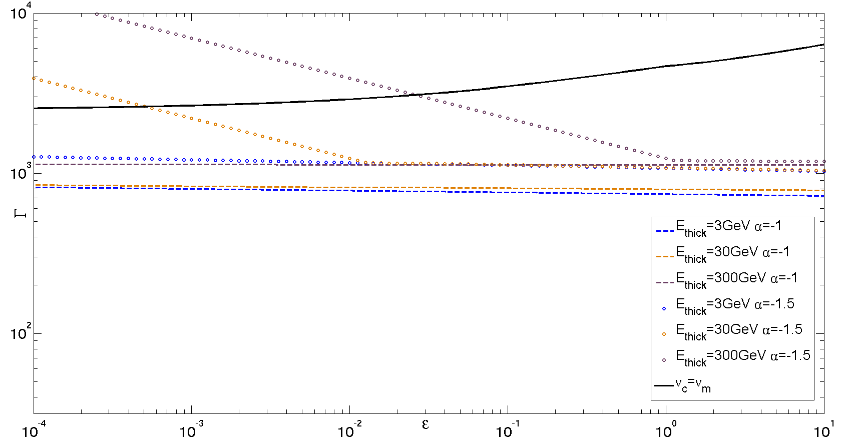
Figure 13: Lower limits on $\Gamma$ from the combined constraints on up-scattered flux and pair creation opacity shwon along with the upper limit on $\Gamma$ originating from $\nu_{c}=\nu_{m}$ for various values of the lower spectral slope ($\alpha$) and the photon energy at which the system becomes optically thick to pair creation ($E_{thick}$). The area above between the dashed or dotted lines and the solid line is allowed by observations. Left panel: $k=1$, right panel: $k=10$.

6 Implications of CTA observations on the Synchrotron model

It is interesting to explore the implications of future GRB observations by the CTA, in the tens of GeV to tens of TeV energy range, on the synchrotron model. The universe is optically thick to radiation above a few hundred GeV (Nikishov, 1962; Gould et al., 1966) and it will therefore be difficult to observe GRBs from typical redshifts $z\approx 1$ in this energy range. However, the CTA is expected to have better detectability in the tens of GeV range than LAT by at least four orders of magnitude (CTA consortium, 2010, 2011). There are three possible scenarios regarding observations of the prompt emission by CTA, schematically drawn in Fig. 14. Least intriguing is a null detection. This could happen either because the system is optically thick to intrinsic pair creation at lower frequencies than the CTA band (i.e. the breaks in the LAT spectrum are due to optical depth for pair creation, and the fact that we do not see anything with CTA is trivially expected) or because the breaks in the LAT spectrum are intrinsic spectral breaks due to the maximal synchrotron frequency and there is simply a very low SSC signal at the CTA band. The latter case could provide significant constraints on the parameters of the model. However, since we cannot rule out a large optical depth, we won’t obtain new constraints on the model just from a null detection. Second, there might be a weak signal in the tens of GeV range which is, however, significant enough to show that the system is optically thin at least up to the CTA band. In this scenario we may associate the LAT breaks with the maximal synchrotron frequency and may obtain $\Gamma$ according to Eq. 33 up to the numerical factor $f$ which is expected to be of order unity. In addition, the improved sensitivity of CTA in the tens of GeV range (relative to that of LAT), could possibly allow us to rule out a wide range of SSC solutions (the SSC component should be both weak and peak at higher frequencies than $\nu_{max}$ for the SSC solution to be compatible with such observations). Effectively, the improved sensitivity would increase the lower limit on $\Gamma$ given by Eq. 39, by replacing $\nu_{max}$ by the maximal photon energy observed with the CTA and replacing the fractional flux detected by LAT, $\eta_{LAT}$ with the corresponding fraction $\eta_{CTA}$ that could be lower by up to two or three orders of magnitude (depending on the actual flux that would be detected by CTA and on the new $\nu_{max}$). This would narrow down the allowed parameter space and would produce lower limits on $\Gamma$ and $\epsilon$. For instance, a detection of even a few photons in the tens of GeV range, could lead to $\epsilon>0.3$ and $\Gamma>500$. Finally, a strong signal, with a fluence larger than the extrapolated LAT emission (i.e. with approximately $10^{-7}ergs/cm^{2}$), detected by the CTA would imply a detection of a new component in this energy band. Such a component, if it ascosiated with the same emitting region, can naturally be explained as the SSC peak If the detection is strong enough, it would allow us to measure both the peak flux and the peak frequency (see §3.3). This will allow, in turn, to determine $\nu_{KN}$ and $F_{SSC}$ and eventually to estimate also $\Gamma$ and $\epsilon$, and hence all other parameters of the system up to $k$. In case there values turn out to be outside the limits on the parameter space ($\nu_{m}>\nu_{c}$, $\tau>1$ etc.) described in §3.2 these measurements could possibly rule out the synchrotron solution. In addition if we can measure $\nu_{syn,max}$ we may obtain another equation and obtain the full solution of the model.

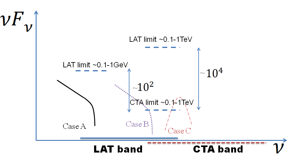
Figure 14: The three possibilities for CTA observations, described in the text. Case A: No signal in the CTA - no significant costraints on the parameter space (as this could be due to optical depth). Case B: a weak signal at tens of GeV, where the CTA is much more sensitive than LAT, leading to strong constraints on SSC. Case C: a detection of a peak (in $\nu F_{\nu}$) in the CTA band, leading to a full solution of the SSC model or ruling it out.

7 Conclusions

We examined the allowed parameter space for the synchrotron emission for the prompt phase of GRBs. We considered individual pulses as the building blocks and demanded that the system is fast cooling with the peak ($\nu F_{\nu}$) frequency comparable to $\nu_{m}$ so that the system can generate the observed flux efficiently. Our discussion is general and it does not depend on the specific energy generation or particle acceleration mechanism.

We characterize the possible parameter space in terms of two parameters: the ratio of magnetic to electron’s energy, $\epsilon$ and the bulk Lorentz factor, $\Gamma$. A third auxiliary parameter is $k$, the ratio between the shell crossing time, and the angular timescale. Efficiency considerations alone limit the ratio of $\epsilon$: $10^{-4}<\epsilon<10$ (see §3.5). The upper limit arises from the requirement that a large fraction of the total kinetic energy has to be stored at some stage in the relativistic electrons ($\epsilon_{e}\gtrsim 0.1$) and thus be available for radiation. The lower limit arises from the requirement that the up-scattered inverse Compton radiation does not dominate over the energy of the observed sub-MeV pulse. The lower limit becomes more stringent for shorter pulses and softer pulses (for example, $t_{p}\approx 5\times 10^{-2}$sec, $\nu_{p}\approx 100$KeV lead to $8\times 10^{-3}<\epsilon<10$). Another implication of efficiency requirements is that soft - high luminosity bursts require huge intrinsic powers in the synchrotron model. This may explain why such bursts are not observed.

Efficiency also constrains $\Gamma$. The upper limit is determined by the condition that the emission process is efficient, namely that $\nu_{c}\lesssim\nu_{m}$. This is more constraining for small values of $\epsilon$ and therefore it suggests rather strong magnetization. The lower limit on $\Gamma$ arises from limits on the SSC component and from opacity considerations. These lead to $150<\Gamma<3000$. Both the limits increase slightly with k, namely when the emitting radius is larger compared with the radius implied by variability. It is interesting to observe (see e.g. Figs. 3,4) that within the allowed solution $\Gamma$ is not necessarily correlated with $\epsilon$).

Current Observations of high energy (GeV) photons lead to pair opacity constraints and to a larger lower limit on $\Gamma$. However, this limit depends on the fact that the high frequency photons originate at the same site as the sub-MeV photons (or at smaller radii) and it maybe relaxed if this is not the case. The observations of high energy photons actually only produces lower limits on the true frequency at which the system becomes optically thick for pair creation ($\nu_{thick}$). We find that if, in reality, this frequency is as high as 300GeV, then low $\alpha$ bursts push the model further towards equipartition ($\epsilon>5\times 10^{-3}$ for $k=1$ or $\epsilon>5\times 10^{-2}$ for $k=10$).

We explore the implications on the synchrotron model of future high energy observations by the CTA, in the tens of GeV to tens of TeV energy range. We find three general possibilities. Most trivially, a null detection by CTA does not yield significant constraints on the model. Second, a weak detection would imply that $\nu_{thick}$ is at least of the order of tens of GeV, and that there is a weak SSC signal up to this frequency. This increases the lower limits on $\Gamma$ and $\epsilon$. Depending on the actual flux measured, these limits can be as strong as $\epsilon>0.3$ and $\Gamma>500$. Third, a strong signal in the CTA band (above the extrapolation of the LAT signal) would be suggestive of an SSC peak. This could allow us to determine at least two of the three free parameters of our model ($\Gamma$, $\epsilon$, $k$) and effectively determine the full solution or possibly rule out the synchrotron model in case either of the first two parameters turns out to be beyond the limits discussed in this paper.

Even though we don’t have a full solution we can obtain a reasonable estimate of the expected range of synchrotron parameters needed to produce the observed prompt emission. The emission radius, $R$, is relatively large: $10^{15}\mbox{cm}<R<10^{17}\mbox{cm}$ and it is independent of $\epsilon$. The magnetic field, $B$, spans almost four orders of magnitude: $3\mbox{ Gauss}<B<10^{4}\mbox{ Gauss}$. The lines of constant $B$ are almost parallel to the $\nu_{m}=\nu_{c}$ line. Larger values of B lead to faster cooling so that the value of $B$ is almost proportional to $x_{ins}$, the ratio between the number of instantaneously emitting relativistic electrons and the overall number of relativistic electrons. The allowed range for $\gamma_{m}$ is: $3\times 10^{3}<\gamma_{m}<10^{5}$. These large values of $\gamma_{m}$ (compared with $m_{p}/m_{e}$) imply that, in many cases, as we discuss below, only a small fraction of the electrons ($10^{50}<N_{e}<10^{52}$) are accelerated to relativistic velocities and participate in the synchrotron emission process. These large values of $\gamma_{m}$ also suggest that any SSC peak would be at energies of at least a few hundred GeV. This is above the LAT band, naturally causing the SSC signal to be hard to observe with current detectors. Interestingly these parameter ranges, are very weakly dependent on $k$ and they remain within this range as long as we keep the observed quantities at their canonical values.

Slightly deviating from the generic approach we present here, we examined the implications of the model if most of the energy is stored at some stage in the form of kinetic bulk motion. This would be naturally the case in the internal shocks model but also if the jet is initially Poynting flux dominated but it converts it energy to kinetic energy before the energy is radiated away. In this case the synchrotron solution requires that only a small fraction of the electrons in the flow are heated by the shocks and dissipate their energy during the prompt emission (Daigne $\&$ Mochkovitch, 1998; Bošnjak et al., 2009). However, we note that the distribution of electrons needed for this type of solution is different than what was achieved by recent PIC simulations, as it requires a gap between the energy of the non-accelerated electrons, and the minimal energy of the power-law component (see 10). We find that the fraction of accelerated electrons, $\xi$ must satisfy $\xi\lesssim 4\times 10^{-2}k^{1/2}$ for a proton dominated flow (see Fig. 4) and $\xi\lesssim 2\times 10^{-5}k^{1/2}$ (Fig. 11) for a pair dominated flow.

The main caveat of this model, that we did not address here, remains the “line of death“ problem, regarding the low energy spectral slope (see also Daigne et al. 2011). A partial solution to this problem can be achieved if the system emits in a marginally fast cooling regime, where $\nu_{m}\approx\nu_{c}$. The high $\Gamma$ values required by opacity considerations, push the model towards this regime. However, even the marginally fast solution, only steepens $\alpha$ up to $-2/3$ and it does not solve the entire problem. A different option is to have a steepening of the slope due to high self absorption frequency (Granot et al., 2000). This is not easily achieved, as the self absorption frequency is typically four orders of magnitude below the peak.

Overall we conclude that there is reasonable range in the parameter ($\Gamma$ and $\epsilon$) phase space for which a synchrotron solution that fits the peak frequency and the peak flux is possible. The main characteristics of this solution are large emission radii, relatively high magnetization and large values of electrons’ Lorentz factors. These Lorentz factors naturally explain the lack of a SSC signal within the LAT band. In addition, the solution naturally explains the lack of soft - high luminosity bursts. Possible future detections of a SSC signal at higher frequencies, will allow to either obtain the full solution of the model, or rule it out altogether.

We thank Jonathan Granot, Rodolfo Barniol Duran and Indrek Vurm for many helpful discussions. The research was supported by an ERC advanced research grant (GRB).

References

- (1)
- Abdo et al. (2009a) Abdo A. A., et al., 2009a, Science, 323, 1688.
- Achterberg et al. (2001) Achterberg, A., Y. A. Gallant, J. G. Kirk, and A. W. Guthmann, 2001, Mon. Not. RAS 328.
- Ackermann et al. (2011) Ackermann, M., et al., 2011, ApJ, 729, 114A.
- Ackermann et al. (2012) Ackermann, M., et al., 2012, ApJ, 754, 121T.
- Aharonian et al. (2009) Aharonian, F.-A., et al. 2009, AA, 495, 505.
- Albert et al. (2006) Albert, J. et al. 2006, ApJ, 641, L9.
- Amati et al. (2002) Amati, L., 2002, AA, 390, 8189.
- Ando et al. (2008) Ando, S., Nakar, E. Sari, R. 2008, ApJ 689, 1150.
- Atkins et al. (2005) Atkins, R. et al. 2005, ApJ, 630, 996.
- Axelsson et al. (2012) Axelsson, M., et al. 2012, ApJ, 757, L31.
- Band (1993) Band, D., et al. 1993, ApJ, 413, 281.
- Band (2005) Band, D. L., Preece, R. D. 2005, ApJ, 627, 319.
- Barniol Duran Kumar (2011) Barniol Duran, R. Kumar, P., 2011, MNRAS 412, 522.
- Barniol Duran et al. (2012) Barniol Duran, R., Bošnjak Ž., Kumar, P. 2012, MNRAS, 424, 3192.
- Bednarz et al. (1998) Bednarz, J., and M. Ostrowski, 1998, Physical Review Letters, Volume 80, Issue 18, May 4, 1998, pp.3911-3914 80, 3911.
- Belborodov (2000) Beloborodov, A. M., 2000, Ap. J. Lett., 539, L25.
- Beniamini et al. (2011) Beniamini, P., Guetta, D., Nakar, E., Piran., T. 2011, MNRAS, 416:3089.
- Beniamini Piran (2013) Beniamini, P., Piran., T. In prep. 2013.
- Bošnjak et al. (2009) Bošnjak, Ž., Daigne, F., and Dubus, G. AA 498, 677 (2009).
- Brainerd (1994) Brainerd, J.J., 1994, in AIP Conf. Proc. 307: Gamma-Ray Bursts, pp. 346.
- Brainerd et al. (1999) Brainerd, J.J., Pendleton, G.N., Mallozzi, R.S., Briggs, M.S. Preece, R.D. 1999, in The 5th Huntsville Gamma-Ray Burst Symposium: Conference Proceedings, 526, 150.
- Cohen et al. (1997) Cohen, E., J. I. Katz, T. Piran, R. Sari, R. D. Preece, and D. L. Band, 1997, Ap. J., 488,330+.
- Crider et al. (1997) Crider, A., Liang, E. P., Smith, I. A., Preece, R. D., Briggs, M. S., Pendleton, G. N., Paciesas, W. S., Band, D. L., Matteson, J. L. 1997, ApJ, 479
- CTA consortium (2010) CTA Consortium 2010, arXiv:1008.3703.
- CTA consortium (2011) CTA Consortium 2011, arXiv:1111.2183.
- Curran (2010) Curran et al. 2010, ApJ 716, L135.
- Daigne et al. (2011) Daigne F., Bošnjak Ž., Dubus G., 2011, AA, 526, A110.
- Daigne Mochkovitch (1998) Daigne, F., and R. Mochkovitch, 1998, Mon. Not. RAS 296, 275.
- Daigne Mochkovitch (2002) Daigne, F., and R. Mochkovitch, 2002, Mon. Not. RAS 336, 1271D.
- Derishev (2003) Derishev E.V., Kocharovsky V.V., Kocharovsky Vl.V., Mészáros P., 2003, in Ricker G.R., Vanderspeck R.K., eds, AIP Conf. Proc., Vol. 662, Gamma-Ray Burst and Afterglow Astronomy 2001: A Workshop Celebrating the First Year of the HETE Mission. Am. Inst. Phys., New York, p. 292
- de Jager (1996) de Jager, O. C., A. K. Harding, P. F. Michelson, H. I. Nel, P. L. Nolan, P. Sreekumar, and D. J. Thompson, 1996, Ap. J., 457, 253.
- Eichler Levinson (2000) Eichler D., Levinson A., 2000, ApJ, 529, 146.
- Fan et al. (2006) Fan, Y. Z. Piran, T. 2006, MNRAS, 369, 197.
- Fenimore et al. (1993) Fenimore, E. E., Epstein, R. I., Ho, C. 1993, AAS, 97, 59.
- Gallant Achterberg (1999) Gallant, Y. A., and A. Achterberg, 1999, Mon. Not. RAS 305, L6.
- Ghirlanda et al. (2002) Ghirlanda, G., Celotti, A., Ghisellini, G. 2002, AA, 393, 409.
- Ghisellini and Celotti (1999) Ghisellini, G., Celotti, A., 1999, ApJ, 511, L93.
- Ghisellini et al. (2000) Ghisellini, G., A. Celotti, and D. Lazzati, 2000, Mon. Not. RAS 313, L1.
- Giannios (2006) Giannios D., 2006, AA, 457, 763.
- Gould et al. (1966) Gould R J and Schréder G 1966 Physical Review Letters 16 252-4
- Granot et al. (1999) Granot, J., Piran, T., Sari, R., 1999, ApJ, 513, 679.
- Granot et al. (2000) Granot, J., Piran, T., Sari, R. 2000, ApJ, 534, L163.
- Granot et al. (2002) Granot J., Sari R., 2002, ApJ, 568, 820.
- Granot et al. (2006) Granot, J., Konigl, A., Piran, T., 2006, MNRAS, 370, 1946.
- Granot et al. (2008) Granot, J., et al. 2008, ApJ, 677, 92.
- Granot et al. (2009) Granot J., Fermi LAT f. t., GBM collaborations 2009, arXiv:0905.2206.
- Granot et al. (2010) Granot, J., for the Fermi LAT Collaboration, the GBM Collaboration 2010, arXiv:1003.2452.
- Guetta et al. (2001) Guetta, D., M. Spada, and E. Waxman, 2001, Ap. J., 557, 399.
- Guetta et al. (2011) Guetta, D., Pian, E., Waxman, E. 2011, AA, 525, 53.
- Guiriec et al. (2011) Guiriec, S., et al. 2011, ApJL, 727, L33.
- Guiriec et al. (2012) Guiriec, S. et al. 2012, ApJ, submitted (arXiv:1210.7252).
- Hascoët et al. (2012) Hascoët, R., Daigne, F., Mochkovitch, R. and Vennin, V. 2012, MNRAS 421, 525H.
- Kaneko (2006) Kaneko, Y., Preece, R. D., Briggs, M. S., et al. 2006, ApJS, 166, 298.
- Katz (1994) Katz, J.I., 1994, ApJ, 422, 248.
- Klotz (2009) Klotz, A., Boër, M., Atteia, J. L., Gendre, B. 2009, AJ, 137, 4100.
- Kobayashi et al. (1997) Kobayashi, S., T. Piran, and R. Sari, 1997, Ap. J., 490, 92+.
- Kobayashi et al. (2001) Kobayashi, S., Sari, R. 2001, ApJ, 551, 934
- Kumar McMahon (2008) Kumar, P. McMahon, E. 2008, MNRAS, 384, 33.
- Lazzati et al. (2003) Lazzati, D., et al., 2003, MNRAS, 347, L1.
- Lithwick Sari (2001) Lithwick Y., Sari R., 2001, ApJ, 555, 540.
- Mallozzi et al. (1995) Mallozzi, R. S., et al. 1995, ApJ, 454, 597
- Rees and Mészáros (1994) Rees, M.J., Mészáros, P., 1994, ApJ, 430, L93.
- Mészáros Rees (2000) Mészáros, P. Rees, M. J. 2000, ApJ, 530, 292.
- Nava et al. (2011) Nava, L., Ghirlanda, G., Ghisellini, G., Celotti, A. 2011, AA.
- Nakar et al. (2005) Nakar E., Piran T., Sari R., 2005, ApJ, 635, 516.
- Nakar and Piran (2005) Nakar, E., Piran, T., 2005, MNRAS, 360, L73.
- Nakar et al. (2009) Nakar, E., Ando, S., Sari, R. 2009, ApJ, 703, 675.
- Nikishov (1962) Nikishov, A.I., 1962, Soviet Phys.JETP, 14, 393.
- Nousek et al. (2006) Nousek, J. A., Kouveliotou, C., Grupe, D., Page, K. L., Granot, J., et al., 2006, ApJ 642, 389.
- O’Brien et al. (2006) O’Brien, P. T., et al. 2006, ApJ, 647, 1213.
- Panaitescu and Kumar (2001) Panaitescu, A., Kumar, P., ApJ, 560, L49.
- Panaitescu and Kumar (2002) Panaitescu, A., Kumar, P. 2002, 571, 779.
- Panaitescu and Kumar (2004) Panaitescu, A., Kumar, P. 20024, MNRAS, 353, 511.
- Peer et al. (2006) Peer, A. Mészáros, P. Rees, M. 2006, ApJ, 642, 995.
- Pelaez et al. (1994) Pelaez, et al. 1994, ApJ, 92, 651.
- Piran (1995) Piran, T., 1995, in Unsolved Problems in Astrophysics.
- Piran (1999) Piran, T. 1999, Phys. Rep., 314, 575.
- Piran Nakar (2010) Piran T., Nakar E., 2010, ApJL, 718, L63.
- Piran et al. (2009) Piran T., Sari R., Zou Y.-C., 2009, MNRAS, 393, 1107.
- Preece et al. (1998) Preece, R.D. et al., 1998, ApJL, 506, 23.
- Preece et al. (2000) Preece, R. D., M. S. Briggs, R. S. Mallozzi, G. N. Pendleton, W. S. Paciesas, and D. L. Band, 2000, Ap. J. Supp., 126, 19.
- Preece et al. (2002) Preece, R.D., et al. 2002, ApJ, 581, 1248.
- Rees Mészáros (2005) Rees, M.-J., Mészáros, P. 2005, ApJ, 628, 847.
- Roming et al. (2006) Roming, P. W. A., et al. 2006, ApJ, 652, 1416.
- Rybicki and Lightman (1979) Rybicki, G.B. and Lightman, A.P., 1979, Radiative Processes in Astrophysics, John Wiley Sons (New York).
- Ryde and Peer (2009) Ryde, F. Peer, A. 2009, ApJ, 702, 1211.
- Sari et al. (1996) Sari, R., Narayan, R., Piran, T. 1996, ApJ, 473, 204.
- Sari and Piran (1997a) Sari, R., Piran, T., 1997, ApJ, 485, 270.
- Sari and Piran (1997b) Sari, R., and T. Piran, 1997, Mon. Not. RAS 287, 110.
- Sari et al. (1998) Sari, R., Piran, T., Narayan, R. 1998, ApJ, 497, L17.
- Sari and Piran (1999) Sari, R., Piran, T., 1997, ApJ, 517, L109.
- Schaefer (2003) Schaefer, B. E., 2003, ApJ, 583, L71.
- Shaviv and Dar (1995) Shaviv, N.J., Dar, A., 1995, ApJ, 447, 863.
- Shahmoradi (2010) Shahmoradi A., Nemiroff R., 2010, Monthly Notices of the Royal Astronomical Society, 407, 2075
- Shemi (1994) Shemi, A., 1994, MNRAS, 269, 1112.
- Shen (2006) Shen et al. 2006, MNRAS 371, 1441.
- Starling (2008) Starling et al.2008, ApJ 672, 433.
- Thompson et al. (2007) Thompson, C., Mészáros, P., Rees, M. J. 2007, ApJ, 666, 1012.
- Vurm et al. (2012) Vurm, I., Lyubarski, Y., Piran, T., 2012, ApJ, in prep.
- Vurm et al. (2012a) Vurm, I., Granot, J., Piran, T., 2012, in prep.
- Wang (2009) Wang et al. 2009, ApJ, 698, L98.
- Waxman (1997) Waxman, E., 1997, ApJ, 485, L5+.
- Wijers and Galama (1999) Wijers, R.A.M.J., Galama, T.J., 1999, ApJ, 523, 177.
- Woods and Loeb (1995) Woods, E., Loeb, A. 1995, ApJ, 453, 583.
- Yonetoku et al. (2004) Yonetoku, D., et al., 2004, ApJ, 609, 935.
- Yonetoku et al. (2010) Yonetoku, D., Murakami, T., Tsutsui, R., Nakamura, T., Morihara, Y., Takahashi, K. 2010,PASJ, 62, 1495.
- Yost et al. (2007) Yost S. A., et al., 2007, ApJ, 669, 1107.
- Zhang et al. (2006) Zhang, B., Fan, Y. Z., Dyks, J., Kobayashi, S., Mészáros, P., et al., 2006, ApJ 642, 354.
- Zhang et al. (2009) Zhang, B., Pe’er, A. 2009, ApJ, 700, L65.
- Zou et al. (2009) Y.-C. Zou, T. Piran, R. Sari, ApJL 692, L92 (2009).
- Zou et al. (2011) Zou Y.C., Fan Y.Z., Piran T., 2011, ApJ, 726, L2.