Atmospheric composition of weak G band stars: CNO and Li abundances

Abstract

We determined the chemical composition of a large sample of weak G band stars – a rare class of G and K giants of intermediate mass with unusual abundances of C, N, and Li. We have observed 24 weak G band stars with the 2.7 m Harlan J. Smith Telescope at the McDonald Observatory and derived spectroscopic abundances for C, N, O, and Li, as well as for selected elements from Na - Eu. The results show that the atmospheres of weak G band stars are highly contaminated with CN-cycle products. The C underabundance is about a factor of 20 larger than for normal giants and the ¹²C/¹³C ratio approaches the CN-cycle equilibrium value. In addition to the striking CN-cycle signature the strong N overabundance may indicate the presence of partially ON-cycled material in the atmospheres of the weak G band stars. The exact mechanism responsible for the transport of the elements to the surface has yet to be identified but could be induced by rapid rotation of the main sequence progenitors of the stars. The unusually high Li abundances in some of the stars are an indicator for Li production by the Cameron-Fowler mechanism. A quantitative prediction of a weak G band star’s Li abundance is complicated by the strong temperature sensitivity of the mechanism and its participants. In addition to the unusual abundances of CN-cycle elements and Li we find an overabundance of Na that is in accordance with the NeNa chain running in parallel with the CN-cycle. Apart from these peculiarities the element abundances in a weak G band star’s atmosphere are consistent with those of normal giants.

I. Introduction

Theoretical and observational investigations of solar metallicity G and K giants have led to broad agreement about the changes in surface composition arising from the first dredge-up initiated by the deep convective envelope of the giant. Principal effects are a drastic lowering of the Li abundance, a reduction of the ¹²C abundance, a lowering of the ¹²C/¹³C ratio and an increase of the ¹⁴N abundance with a preservation of the sum of ¹²C, ¹³C, and ¹⁴N nuclides.

Rare examples of G and K giants exhibiting startling departures from the broad agreement shared by the vast majority of the stars highlight the fact that facets of the evolution of these stars from birth to the giant branch have eluded theoretical understanding. Weak G band stars (here, wk Gb stars) are just such a class of exceptional stars. The discovery of the first of these stars showing weak CH molecular lines in the Fraunhofer G band was made by Bidelman (1951) who examined low-resolution spectra of HR 885 and remarked ‘the spectrum is extraordinarily peculiar, with the line spectrum matching fairly well G5 III but with no trace of CN or CH absorption’. A quantitative analysis from coudé spectra was undertaken by Greenstein & Keenan (1958) who not only found both CH and CN deficient by about 2 dex but uncovered a second wk Gb star – HR 6791 – with less extreme CH and CN deficiencies.

Bidelman & MacConnell (1973) laid the groundwork for an extensive abundance analysis of wk Gb stars with a search of objective prism plates aimed at finding ‘the brighter stars of astrophysical interest’ which provided a list of 34 stars with ‘weak or no G band’. The survey forming the basis for the list was focused on the southern hemisphere and, hence, did not include either HR 885 or HR 6791. Although the 1973 paper has been followed by several papers discussing aspects of quantitative abundance analyses of wk Gb stars, there has, apart from determinations of the Li abundance, been no comprehensive analysis of elements and isotopes (i.e., C, N, and O in particular) which should be useful diagnostics of the causes of the weak G band phenomenon. Notably, Palacios et al. (2012) in their compilation of published abundances for 28 wk G band stars list Li abundances for 18 stars but C and N abundances for just four stars and O abundances for only two stars ( taken from Sneden et al. 1978, Cottrell & Norris 1978, and Day 1980).

The principal aim of our paper is to provide the first thorough abundance analyses of a complete sample of the wk Gb stars accessible to us at the W.J. McDonald Observatory in Texas. Our focus is on the determination of the Li, C, N, and O abundances and the ¹²C/¹³C ratio but other elements from Na to Eu are also included. Such data are considered by us to be a prerequisite to a discussion of likely origins of this class of peculiar red giants. Of the variety of origins proposed in the literature, none seems to account convincingly for the reported abundance data.

II. Observations

We observed 24 wk Gb stars with the 2.7 m Harlan J. Smith Telescope at the McDonald Observatory. The telescope was equipped with the Robert G. Tull Cross-Dispersed Echelle Spectrograph (Tull et al. 1995) and a Tektronix 2048 x 2048 pixel CCD detector. A majority of the stars was observed with two different setups of the Tull spectrograph. The pair when combined provide coverage of the inter-order echelle gaps. The blue setup was centered on 5112 Å in order 68, while the red setup is centered on 5178 Å (order 68). A few stars were observed in what we deem the standard (std) setup centered on 5060 Å in order 69. For all setups a wavelength range of 3 900–10 000 Å was covered with a resolving power of $\text{R}\equiv\lambda/\Delta\lambda=60\,000$. The observations are listed in Table 1. The spectra were reduced in a multiple step procedure. First flat field and bias corrections were applied. Then the echelle spectra were extracted and wavelength calibrated using ThAr-lamp comparison exposures taken before or after the observations. The different spectral orders were co-added and continuum normalized. All tasks were performed using the IRAF package .

Table 1Observation log of analyzed spectra. The different setups are described in the text.

Object	Obs. date (UT time)	$t_{\text{e}xp}$[s]	setup
37 Com	Feb 19 2011	$600$	red
	Feb 20 2011	$600$	blue
BD +5∘593	Feb 19 2011	$3\times 1\,800$	red
	Feb 20 2011	$3\times 1\,800$	blue
HD 18636	Nov 15 2011	$3\times 1\,200$	red
	Nov 16 2011	$3\times 1\,200$	blue
HD 28932	Nov 15 2011	$4\times 1\,200$	red
	Nov 16 2011	$4\times 1\,200$	blue
HD 31869	Nov 16 2011	$4\times 1\,200$	blue
HD 40402	Nov 16 2011	$3\times 1\,200$	blue
	Nov 17 2011	$2\times 1\,800$	std
HD 49960	Nov 15 2011	$3\times 1\,200$	red
	Nov 16 2011	$4\times 1\,200$	blue
HD 67728	Feb 19 2011	$2\times 1\,800$	red
	Feb 20 2011	$2\times 1\,800$	blue
HD 78146	Feb 19 2011	$3\times 1\,800$	red
	Feb 20 2011	$3\times 1\,800$	blue
HD 82595	Feb 19 2011	$2\times 1\,800$	red
	Feb 20 2011	$2\times 1\,800$	blue
HD 94956	Feb 19 2011	$2\times 1\,800$	red
	Feb 20 2011	$2\times 1\,800$	blue
HD 120170	Feb 19 2011	$3\times 1\,800$	red
	Feb 20 2011	$3\times 1\,800$	blue
HD 120171	Feb 19 2011	$3\times 1\,800$	red
	Feb 20 2011	$3\times 1\,800$	blue
HD 132776	Mar 07 2012	$2\times 1\,800$	blue
	Mar 08 2012	$2\times 1\,800$	red
HD 146116	Mar 07 2012	$2\times 1\,200$	blue
	Mar 08 2012	$3\times 1\,800$	red
HD 188028	Sep 24 2012	$1\,200+1\,800$	blue
	Sep 25 2012	$1\,200+1\,800$	red
HD 204046	Nov 16 2011	$3\times 1\,200$	blue
	Nov 17 2011	$3\times 1\,200$	red
HD 207774	Nov 15 2011	$4\times 1\,200$	red
	Nov 16 2011	$4\times 1\,200$	blue
HR 885	Feb 21 2011	$900$	std
HR 1023	Feb 21 2011	$1\,200$	std
HR 1299	Nov 15 2011	$2\times 1\,200$	red
	Nov 16 2011	$2\times 1\,200$	blue
HR 6757	Feb 19 2011	$2\times 1\,200$	red
	Feb 20 2011	$2\times 1\,200$	blue
HR 6766	May 14 2011	$360$	red
	May 14 2011	$300$	blue
HR 6791	May 14 2011	$360$	red
	May 14 2011	$360$	blue

III. Parameter determination

III.1. Spectroscopic

The parameters of the program stars were derived by spectroscopic means using Fe i and Fe ii lines. The line selection process included the comparison of different line lists and atomic data. The original line list composed for this purpose contained about 280 Fe i and 25 Fe ii lines that we identified in the wk Gb spectra by comparison with the solar atlas. Values for the ${\log gf}$ values of these lines were taken from NIST , the Kurucz database (Kurucz & Bell 1995), and Meléndez & Barbuy (2009). The line equivalent widths (EWs) were measured with an Automatic Routine for line Equivalent widths in stellar Spectra (ARES, Sousa et al. 2007). Lines not found, or not identified as single lines by ARES, were removed from the list. As a next step, the measured EWs were plotted against the strength of the lines, i.e. roughly the difference of ${\log gf}$ and excitation potential $\chi$, in order to identify and remove lines, which deviate too strongly from the linear trend. The resulting line list was then used as input for the spectral synthesis code MOOG (Sneden 1973) for an abundance analysis. We made use of input model atmospheres, which were interpolated from a grid of models from Castelli & Kurucz (2004). Assuming a one-dimensional, plane-parallel atmosphere in local thermodynamic equilibrium (LTE), the abundances of the computed lines were force-fitted to match the measured EWs. The derived abundances were plotted vs. the excitation potential of the lines and any trend was flattened by adjusting the effective temperature (${T_{\text{eff}}}$) of the model atmosphere. Simultaneously, the microturbulence was derived by reducing the trend in the plot of Fe abundances and reduced equivalent width (EW divided by wavelength). The surface gravity was adjusted until abundances derived by Fe i and Fe ii lines matched within 0.12 dex, which for most of the stars corresponds to the standard deviation of the Fe ii abundance. Since all parameters are to some extent interdependent, usually several iterations are needed. In order to minimize the error of the ${T_{\text{eff}}}$ determination, the line list was iteratively cleaned of Fe i and Fe ii lines that showed significant deviations in their abundances compared to the derived average abundance of their species. This was done until the resulting $\sigma$ for the abundance determination was reduced to $\approx$ 0.05. NLTE effects that could affect the determination of Fe abundances and stellar parameters are negligible for G and K stars in our metallicity range (Bergemann et al. 2011, Mashonkina et al. 2011). We repeated the procedure for the line lists presented in Ramírez & Allende Prieto (2011) and Takeda, Sato, & Murata (2008). The former consists of 37 Fe i and 9 Fe ii lines with ${\log gf}$ values from different sources (e.g the Oxford group and Allende Prieto, Lambert, & Asplund 2002, most references can be found in Lambert et al. 1996) and was compiled for the determination of the iron abundance of Arcturus. The latter includes 124 Fe i and 11 Fe ii lines with excitation potential and ${\log gf}$ values from Grevesse & Sauval (1999), and was used for the determination of stellar parameters of late-G giants.

Effective temperatures derived with the line list from Ramírez & Allende Prieto (2011) agree with the temperatures that were derived with our original large line list. The scatter is less than $\pm 100\,\text{K}$. The logarithms of the surface gravities agree within $\pm 0.3\,\text{dex}$. The microturbulence derived with the Ramírez & Allende Prieto (2011) line list is on average higher by about $0.5\,\text{km s}^{-1}$, the metallicity lower by about 0.15 dex.

The temperatures derived with the Takeda et al. (2008) line list are on average lower than the ones derived with the original line list by about 150 K, the ${\log g}$ values are lower by about 0.3 dex, microturbulences are higher by $0.3\,\text{km s}^{-1}$, and metallicities are smaller by about 0.25 dex.

The atomic data for the lines that our original list and Ramírez & Allende Prieto (2011) have in common is almost identical, with differences in the ${\log gf}$ values of $\Delta{\log gf}=-0.031\pm 0.076$. The small discrepancy in the derived parameters is therefore probably a result of the line selection itself. A higher number of lines of a certain excitation potential could have statistical influence on the observed trend of abundance with $\chi$. To test the influence of the number of lines included in a line list, we randomly chose a subset of lines from our original list and repeated the parameter determination. The results, however, did not vary significantly. We decided to compile a final line list out of the line list from Takeda et al. (2008) and Ramírez & Allende Prieto (2011) and include the lines of Meléndez & Barbuy (2009) for additional Fe ii line data. The Kurucz loggf values are computed and might therefore be less accurate. The line lists of Takeda et al. and Ramírez & Allende Prieto are compiled and tested for giant stars and include reliable loggf values. Hence the choice for the final line list. The spectroscopic (sp.) parameters derived with this line list can be found in Table 2.

The uncertainties for the temperatures can be estimated from different sources. Since we typically derived two temperatures for every star, corresponding to the different observing setups (see section II), we take the difference between both derived temperatures as a statistical error. This error is $\approx 30\,\text{K}$. In cases where only one setup was available we assume this error to be 50 K. For each setup we determined an additional error by varying the temperature and investigating the impact on the slope of the trend between Fe i abundances and excitation potential. Varying the temperature by more than 50 K results in a difference in the Fe abundances of lines with low and high excitation potential that is larger than the $1\sigma$ error derived for the Fe abundance with no trend. We take this as our instrinsic error. Adding both errors results in a mean error for the spectroscopic temperatures of 90 K (see Table 2).

For the spectroscopic gravities we estimate a mean error of 0.18 dex from the different gravities derived for each star with the different setups. The metallicities in Table 2 are calculated as the mean value of Fe i and Fe ii abundances, minus the solar Fe abundance of Asplund et al. (2009), $\log\epsilon(\text{Fe})=7.50$ , of all setups that were available for a star. The quoted errors are derived by taking into account the standard deviation of these abundances and the errors for the individual abundance determinations. In cases where only one setup was available we assume an error of 0.1 for the missing abundances.

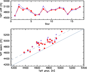
Figure 1.— Top panel: Comparison of ${T_{\text{eff}}}$ ranking for spectroscopic (circles) and LDR temperatures (triangles). Lower panel: Comparison of photometric temperatures lines with spectroscopic ${T_{\text{eff}}}$ determined using Fe i lines (circles) and ${T_{\text{eff}}}$ derived with the line-depth ratio method (triangles). The spectroscopic temperatures are consistently higher than the photometric ones. The dashed line indicates an offset of 200 K from the 1:1 ratio (solid line).

III.2. Line Depth Ratios

To check that our line list gives accurate results for the ${T_{\text{eff}}}$ of our objects we employed additional methods to determine their temperatures. As described in Gray & Brown (2001), line depth ratios (LDRs) of certain elements are excellent indicators of stellar temperatures for G and K giants. Measuring the depth of temperature sensitive V i lines and comparing them to close-by Ni i, Si i and Fe i lines, provides a good tool to constrain the temperatures of the stars. Gray & Brown (2001) calibrated the LDRs against the (B-V) color index and applied corrections for metallicity and absolute-magnitude variations. The (B-V) colors were then converted into temperatures using the temperature scale of Taylor (1999). We use our spectroscopically derived metallicities and parallaxes from the new Hipparcos reduction of van Leeuwen (2007) for the metallicity and absolute-magnitude corrections.

Our temperatures determined by the LDRs measured in the wk Gb stars are in excellent agreement with our spectroscopically derived temperatures, the mean difference being 13 K. It should, however, be noted that the dependence on an original effective temperature scale limits the accuracy of the determination of absolute temperatures derived by the LDR measurements. Nevertheless, the ranking of the stars according to their relative temperatures is not affected and also agrees well with the temperature sequence found for our spectroscopic temperatures (cf. Figure 1). For some stars no LDR temperatures could be derived due to different reasons. For the stars with imprecisely known parallaxes, no correction for absolute-magnitude variations could be made. For 37 Com, HD 67728, and HR 1023, strong line broadening caused difficulties for the LDR measurement. The LDR method depends on a low $v\sin i$ and these three stars are rapid rotators. However, for all stars with measured LDRs the derived temperatures confirm our spectroscopic result and justify our particular choice of line list.

Table 2Atmospheric parameters of the program stars.

Object	${T_{\text{eff}}}$ sp.	$\sigma$	${T_{\text{eff}}}$ ph.	$\sigma$	${\log g}$ sp.	$\sigma$	${\log g}$ ph.	$\sigma$	${v_{t}}$ sp.	[Fe/H] sp.	$\sigma$
	[K]		[K]		[cm s-2]		[cm s-2]		[km s-1]
37 Com	4610	100	4377	34	2.5	0.18	1.9	0.11	2.8	-0.53	0.11
BD +5∘593	5045	60	4820	188	2.5	0.18			1.6	-0.29	0.14
HD 18636	5085	80	4926	57	2.7	0.18	2.8	0.17	1.6	-0.16	0.13
HD 28932	4915	80	4666	62	2.5	0.18	2.3	0.34	1.5	-0.39	0.14
HD 31869	4800	100	4867	82	1.8	0.18	3.2	3.33	1.6	-0.47	0.20
HD 40402	5005	110	4852	73	2.8	0.18	2.6	0.66	1.3	-0.14	0.14
HD 49960	4860	130	4634	81	2.4	0.18	2.0	0.65	1.7	-0.25	0.16
HD 67728	4630	100	4479	41	1.2	0.18	2.2	0.29	1.9	-0.43	0.18
HD 78146	4680	90	4439	75	2.1	0.18	1.8	1.04	1.6	-0.06	0.12
HD 82595	4880	60	4731	57	2.5	0.18	2.6	0.29	1.6	0.06	0.15
HD 94956	4965	60	4786	69	2.5	0.18	2.7	0.41	1.7	-0.19	0.13
HD 120170	4890	90	4693	65	2.4	0.18	4.2	0.66	1.5	-0.51	0.16
HD 120171	4745	120	4725	82	2.3	0.18			1.5	-0.42	0.15
HD 132776	4680	70	4441	130	2.3	0.18	2.0	0.98	1.5	-0.07	0.17
HD 146116	4800	90	4517	70	2.1	0.18	1.8	0.54	1.7	-0.39	0.14
HD 188028	4920	70	4603	90	2.3	0.18	2.1	0.45	1.7	-0.18	0.13
HD 204046	4920	90	4625	158	2.5	0.18	2.4	0.81	1.7	-0.05	0.14
HD 207774	5025	160	4777	17	2.6	0.18	2.8	0.51	1.7	-0.33	0.12
HR 885	4960	100	4902	53	2.1	0.18	2.5	0.06	1.7	-0.35	0.16
HR 1023	5310	100	5020	33	1.6	0.18	2.2	0.25	2.5	-0.22	0.18
HR 1299	4690	60	4640	35	2.2	0.18	2.3	0.11	1.4	-0.08	0.15
HR 6757	4955	60	4592	97	2.5	0.18	2.4	0.11	1.5	-0.08	0.11
HR 6766	4960	70	4818	60	2.4	0.18	2.4	0.04	1.7	-0.18	0.14
HR 6791	5080	90	4928	61	2.6	0.18	2.5	0.08	1.5	0.00	0.15

III.3. Photometric

A multitude of different sources for photometric data and calibrations exist. One of the most often applied is the calibration from Alonso, Arribas, & Martínez-Roger (1999). In order to derive precise and accurate photometric temperatures we try to derive temperatures from as many colors as possible and use only quality photometric data. We employ the General Catalogue of Photometric Data (GCPD, Mermilliod, Mermilliod, & Hauck 1997) as well as ground-based V magnitudes included in the Hipparcos-Tycho catalogue (ESA 1997). Infrared colors from the Two Micron All Sky Survey (2MASS) were also used, if the observations were not saturated, and transformed into the TCS (Telescopio Carlos Sánchez) system used by Alonso et al. (1999). We also made use of the calibration of Ramírez & Meléndez (2005). They offer calibrations for a lot of different photometric systems including UBV, uvby, Vilnius, Geneva, and DDO in addition to the systems included in the Alonso et al. (1999) calibrations. Also, the calibrations of Ramírez & Meléndez (2005) avoid uncertainties due to color-color transformations. For all calibrations we used our spectroscopically determined metallicities.

The temperatures derived from the (B-V) color indices with the calibration of Alonso et al. (1999) agree well with the corresponding temperatures derived with the Ramírez & Meléndez (2005) calibrations, the mean difference being lower than 10 K. For the (V-K) colors differences are $\approx 20\,\text{K}$. These are the only indices that both calibration have in common. The photometric temperatures derived from different systems show some scatter. It is possible that the weak G band in our objects is affecting the photometric colors - directly, or indirectly. A direct effect is most serious for colors from the DDO system (McClure & van den Bergh 1968). The temperatures derived from this system are higher than the ones derived from all other systems. Ramírez & Meléndez (2005) report a strong metallicity dependence for the DDO colors, however, the main reason for the discrepancy is that the giant sample that Ramírez & Meléndez (2005) used to calibrate the Teff scale is dominated by stars with normal G-band. This leads to a lack of absorption in the 42 filter and makes the star bluer and therefore hotter (Ramírez, priv. comm.). Our final photometric temperatures are derived by averaging all available temperatures without including those derived by the DDO colors whenever possible . They can be found in Table 2 together with their errors, which are simply the standard deviations of the mean temperatures.

The photometric temperatures are consistently lower by 194 K than the spectroscopic ones (see lower panel of Figure 1). It is not clear where the offset between spectroscopic and photometric temperatures originates. A similar comparison between photometric temperatures derived with (B-V) colors and spectroscopic temperatures in Takeda et al. (2008) shows a dispersion of comparable size but no systematic offset. Interestingly, in the paper of Luck & Heiter (2007) on giants in the local region, the authors find an offset of 98 K between their spectroscopic temperatures derived with the newest MARCS models and their photometrically derived temperatures. This offset increases by another 50 K when using the older MARCS75 model atmospheres. Baines et al. (2010) present spectroscopic temperatures for 25 K giants. We determined photometric temperatures for their objects and find that the spectroscopic temperatures are higher by about 80 K. These comparisons show that higher spectroscopic temperatures are not specific to the wk Gb stars. Their main characteristic, the weak absorption at wavelengths around 4300 Å, might affect single colors only (mainly B, and the 42 filter of the DDO system). However, the higher flux in these filters would only increase the photometrically derived temperatures, and thus, minimize the difference between the temperatures.

It should be noted that the differences in the temperatures derived with the different methods presented here are not critical to the analysis and results described in the following sections. The differences in the derived abundances (see sections IV.1-IV.5) are subtle and do not affect the overall conclusions derived in these sections and discussed in sections V and VI.

III.4. Reddening, mass, and luminosity

We estimated the reddening of our stars similar to the procedure described in Luck & Heiter (2007). First we calculate the reddening of our stars with the EXTINCT code provided by Hakkila et al. (1997), using the position of our objects and the distances calculated from the Hipparcos parallaxes as input. Then we subtract the reddening calculated for a distance of 75 pc accounting for the reddening-free Local Bubble.

Most of our objects are not affected by reddening. Over 50% of the sample stars have a reddening lower than $E(B-V)=0.025$ which corresponds to a change in ${T_{\text{eff}}}$ of $\approx+50\,\text{K}$ for the (B-V) colors. The determination of the reddening in most of the other cases suffers from uncertain parallaxes and large errors in the determined total visual extinction, sometimes far exceeding the actual values. We therefore continue under the assumption that reddening is negligible.

We calculated luminosities for the program stars with the Hipparcos parallaxes and the GCPD visual magnitudes and their errors. In the cases where no V magnitude or error estimate was available in the GCPD we take magnitudes and errors from the NOMAD catalogue . We applied a bolometric correction according to Alonso et al. (1999). Using both spectroscopic and photometric temperatures we derived the position of the stars in the Hertzsprung-Russell Diagram (HRD). For some of the stars the errors in the parallaxes are large. Figure 2 shows the location of the wk Gb stars in the HRD and evolutionary tracks from Bertelli et al. (2008, 2009). The errors of the parallaxes of some of our objects are large. We therefore only plot objects with parallax errors smaller than 75% of the actual parallax. Depending on the set of temperatures used, the positions of the objects lead to different conclusions. While the hotter spectroscopic temperatures place the objects at positions at the beginning of the giant branch ascent, the photometric temperatures indicate a more advanced evolution. It is apparent that for the region in the HRD where the wk Gb stars can be found, the exact placement of the stars depends critically on the temperature.

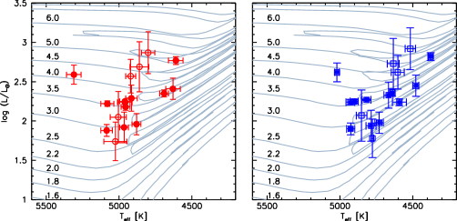
Figure 2.— Program stars with spectroscopically (left panel) and photometrically (right panel) determined ${T_{\text{eff}}}$ in the HRD. Filled symbols mark objects with parallax errors smaller than 50%. Evolutionary tracks, labeled with the respective stellar masses in $M_{\odot}$, were calculated by Bertelli et al. (2008, 2009) for a solar composition ($\text{Z}_{\odot}=0.017$, $\text{Y}_{\odot}=0.260$).

We determined the masses of the program stars by interpolating between the evolutionary tracks of Bertelli et al. (2008, 2009). We do not use a complete isochrone fitting technique and determine probability distribution functions for our masses but rather rely on the evolutionary tracks for a solar composition ($\text{Z}_{\odot}=0.017$ and $\text{Y}_{\odot}=0.260$). Changing the metallicity does not siginifcantly affect the masses of our objects. We make a test calculation for this approach for Arcturus and its parameters given in Ramírez & Allende Prieto (2011) and obtain $M_{\text{A}}=1.47\pm 0.08\,M_{\odot}$ compared to their value of $1.08\pm 0.06\,M_{\odot}$ and justifies our approach. The masses of the wk Gb stars are in the range $2.5-5M_{\odot}$ with a mean mass of $3.56\pm 1.07\,M_{\odot}$.

With the masses of the stars we determined photometric surface gravities using our parameters and the relation

$${\log g}=0.4(M_{\text{bol}}+M_{\text{bol}\,\odot})+{\log g}_{\odot}+4\log\left(\frac{{T_{\text{eff}}}}{{T_{\text{eff}\,\odot}}}\right)+\log\left(\frac{M}{M_{\odot}}\right),$$

with $M_{\text{bol}}=M_{\text{V}}+BC$. We take ${T_{\text{eff}\,\odot}}=5780\,\text{K}$, ${\log g}_{\odot}=4.44$, and $M_{\text{bol}\,\odot}=4.75\,\text{mag}$, as the solar parameters. The photometrically derived gravities are close to the spectroscopic ones, the mean difference being $0.13\pm 0.57$. For some of the stars however, large errors arise from uncertainties in parallaxes (for the calculation of $M_{\text{bol}}$) and masses. For BD +5^∘593 and HD 120171, for example, no ${\log g}$ could be derived at all. We therefore rely exclusively on the spectroscopic gravities in the further analysis. Our derived masses for the wk Gb stars can be found in Table 3. Note that we typically obtain unsymmetrical errors for the masses and quoted the higher ones in the table.

Table 3Distances and masses of the program stars.

Object	plx	$\sigma$	$\sigma$	d	$\sigma$	mass sp.	$\sigma$	mass ph.	$\sigma$
	[mas]		[%]	[pc]		[$M_{\odot}$ ]		[$M_{\odot}$ ]
37 Com	4.94	0.55	11.1	202	23	4.8	0.3	4.3	0.5
HD 18636	3.48	0.57	16.4	287	47	2.9	0.3	2.9	0.3
HD 28932	1.94	0.73	37.6	516	194	3.7	0.7	3.5	1.1
HD 31869	3.90	14.70	376.9	256	967	1.7	8.1	1.9	8.0
HD 40402	1.87	1.39	74.3	535	398	3.2	1.3	3.2	1.5
HD 49960	1.03	0.76	73.8	971	716	4.7	1.8	4.7	2.1
HD 67728	2.16	0.67	31.0	463	144	3.7	0.9	3.2	1.1
HD 78146	0.84	0.99	117.9	1191	1403	5.1	3.2	4.8	4.9
HD 82595	2.58	0.79	30.6	388	119	3.0	0.6	2.6	0.7
HD 94956	2.36	1.07	45.3	424	192	3.0	0.8	2.8	1.0
HD 120170	23.90	13.70	57.3	42	24	0.6	0.3	0.6	0.4
HD 132776	0.89	0.99	111.2	1124	1250	4.6	3.0	4.0	4.9
HD 146116	1.16	0.71	61.2	862	528	5.1	1.6	5.3	2.1
HD 188028	1.56	0.78	50.0	641	321	4.3	1.1	4.3	1.5
HD 204046	1.39	1.27	91.4	719	657	3.4	1.9	2.9	2.7
HD 207774	2.32	1.30	56.0	431	242	2.7	0.9	2.4	1.2
HR 885	6.39	0.35	5.5	157	9	3.6	0.1	3.6	0.1
HR 1023	2.68	0.74	27.6	373	103	4.1	0.6	4.4	0.6
HR 1299	3.80	0.39	10.3	263	27	3.6	0.3	3.5	0.3
HR 6757	4.65	0.48	10.3	215	22	3.5	0.2	3.0	0.4
HR 6766	9.62	0.26	2.7	104	3	3.6	0.1	3.6	0.1
HR 6791	7.96	0.62	7.8	126	10	3.5	0.1	3.6	0.2

IV. Abundances

The focus of the abundance analysis is on those species that may provide clues to the reasons for the weak G band, i.e., the significant underabundance of carbon relative to the slight underabundance of carbon exhibited by giants which have passed through the first dredge-up. If the wk Gb stars’ carbon underabundance is of nucleosynthetic origin, the H-burning CN-cycle is presumably primarily responsible with the expectation that the carbon isotopic ratio ¹²C/¹³C may approach the cycle’s equilibrium value of about 3 and the ¹⁴N will be overabundant but the sum of the nuclides ¹²C + ¹³C + ¹⁴N will be unchanged from its value in the progenitors of the wk Gb stars. A certain expectation for ⁷Li cannot be made but a difference between wk Gb and normal giants is not unexpected. Although Li is readily destroyed by protons at the temperatures required to run the CN-cycle, it may also be produced from existing ³He by the Cameron-Fowler (1971) mechanism: ³He(⁴He)⁷Be($e^{-},\nu)^{7}$Li. The atmospheric Li abundance depends not only on the competition in the interior between production and destruction but also on the transport of Li from the interior production (and destruction) site to the cooler exterior layers where survival is assured.

The abundance analysis should also check the plausible assumption that the H-burning ON-cycles which are effective at higher temperatures than the CN-cycle have not been a determining factor. With optical spectra, this check is possible by determining the ¹⁶O abundance. Additional checks from determinations of the ¹⁷O and ¹⁸O abundances may be possible when spectra of the 4.6$\mu$m CO ground state’s fundamental vibration-rotation band are obtained.

Abundances of other elements are not without interest. Demonstration that the abundances from Na to Eu are normal would serve to restrict the possibility that diffusive processes have operated in a wk Gb star’s progenitor and might be a contributor to the severe carbon underabundance. Although one might suppose the nucleosynthetic possibilities are remote, abundances of heavy elements should be determined to check for unusual contributions from the neutron capture $s$-process (say, Y, La) and $r$-process (say, Eu). An $s$-process enhancement, as in the case of Barium stars, may be possible for a binary star in which a companion as an AGB star dumps material onto the present wk Gb star or its progenitor but, however, the carbon underabundance is not readily explained by this idea. Similarly, a massive companion exploding as a Type II supernovae would certainly leave its nucleosynthetic imprint on the companion.

In the following sections, we describe the abundance analysis and its results. Atomic and molecular data are described in the appropriate sections. At the outset, a comment needs to be made on the molecular equilibrium which affects the partial pressures of C and O and very weakly of N. At the temperatures of these giants, the only molecules of importance are CO and to a far lesser degree N₂. Carbon monoxide with its well determined dissociation energy and partition function affects the partial pressures of C and O in the outer layers of these giants. Thus, these abundances must be obtained iteratively. The derived C abundances are therefore reviewed after the determination of the N and O abundance and vice versa until the changes in the abundances for each element are smaller than 0.1 dex (typically even lower than that). The N₂ molecule, also with a well determined dissociation energy and partition function, has a very minor influence on the partial pressure of N. The H₂ and H₂O molecules exert a totally negligible influence on the partial pressure of H and O.

The abundance analyses are completed with both the spectroscopically and photometrically determined atmospheric parameters. Although the abundances differ in detail, the key differences between wk Gb stars and normal giants are unaffected and presented here for the first time for a complete sample of known wk Gb stars accessible from the northern hemisphere. Interpreting the abundances is a major challenge and not mitigated by the choice of the temperature scale.

For the synthesis of the different features described in the next sections we estimated the external broadening parameters of the lines. We found that the effect of the combination of macroturbulence, rotation, and instrumental profile can be well approximated by a Gaussian function. The fwhm of the Gaussian is derived from different components. The fwhm of the instrumental profile can be determined by measuring the fwhm of emission lines from ThAr spectra. The effect of macroturbulent and rotational velocities is derived by measuring the fwhm of lines in different wavelength regions of the echelle spectra. The determined fwhm for the Gaussian was then tested and adjusted by fitting unblended lines in the vicinity of our lines of interest whenever possible.

The abundances derived in the following sections are summarized in Tables 4 and 5. Table 4 gives the abundances of Li, C, N, and O as well as the ¹²C/¹³C ratio. Elemental abundances are given for the spectroscopic and photometric temperatures for each star. The C isotopic ratio is effectively independent of the temperature scale. Table 5 gives abundances for Na to Eu for both the spectroscopic and photometric temperatures.

IV.1. Carbon

The C depletion of the typical wk Gb star is such that the carbon indicators in optical spectra most often used in the analysis of normal GK giants are unavailable. For example, Luck & Heiter (2007) in their large survey of nearby giants chose the C i 5380 and 6578 Å lines and a feature of the C₂ Swan system at 5135 Å. In the wk Gb stars, these lines are either absent or too weak to provide a useful abundance. Although the C i triplet lines at 9078.28, 9088.51, and 9094.8 Å are present in our spectra, they are blended strongly by telluric H₂O lines such that we do not consider them to be reliable abundance indicators given our spectra.

The CH G band, the A-X system, near 4310 Å in normal giants is strong and saturated. Lambert & Ries (1977, 1981) adopted, as a secondary C abundance indicator a CH feature at 4835 Å comprised of a blend of two 0-1 and a 1-2 A-X line with a strength of about 10 mÅ in a typical and normal GK giant. This feature is weakened below detectable limits in the wk Gb stars. By elimination, the potential C abundance indicators in our optical spectra of wk Gb stars are reduced to CH lines comprising Fraunhofer’s original G band. The G band is not an ideal indicator because of the number of blending features and uncertainties in establishing the continuum but fortunately the molecular data are well determined.

The line list of molecular and blending atomic lines is taken from B. Plez (private communication) for the considered region of 4300-4340 Å. The dissociation energy of CH is well determined: $D_{0}=3.465$ eV (Huber & Herzberg 1979). The $gf$-values of CH lines in Plez’s list are based on band oscillator strengths derived from accurate experimentally determined radiative lifetimes (Larsson & Siegbahn 1986). Asplund et al. (2005) provide a list of nine clean solar CH lines with wavelengths from 4218.72 Å and 4356.60 Å which yield a solar C abundance in satisfactory agreement with the abundance from their primary C abundance indicators ([C i], C i, CH vibration-rotation, and C₂ Swan lines). Their adopted $gf$-values are in excellent agreement with those from Plez; the same recipes appear to have been implemented.

An example of the synthesis of a part of the G band for the wk Gb star HD 18636 is shown in Figure 3. No attempt has been made to fine tune the strengths of atomic lines across the illustrated region; there are a few obvious wavelengths where the blending atomic lines are either too strong or too weak. The best-fitting synthetic spectrum corresponds to a C abundance [C/H] $\simeq-1.6$ when the O abundance is set at the value derived from the [O i] 6300 Å line (see below).

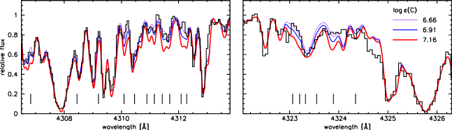
Figure 3.— A fragment of the CH G band in HD 18636 at CH band heads (histogram). Overplotted are synthetic spectra calculated with our spectroscopic temperatures. They show models with the best fitting C abundance of $\log\epsilon(\text{C})=6.91$ and $\pm 0.25\,\text{dex}$. Key CH features are marked with lines below the spectra.

IV.2. Nitrogen

The N abundance is obtained from lines of the CN red ($A^{2}\Pi-X^{2}\Sigma^{+}$) system and, in particular, the 2-0 band near 8000 Å. The 1-0 band is seriously blended with telluric lines and the 3-0 band is rather too weak to be useful. The CN Violet system is too strong and blended to be useful and often recorded with low S/N ratio on our spectra. Of course, measurements of CN lines demand knowledge of the C (and O) abundances in order to obtain the N abundance.

A line list for the Red system was provided by B. Plez (2011, private communication). Wavelengths of the useful lines are recomputed from energy levels given in Ram, Wallace, & Bernath (2010a); Ram et al. (2010b); all adopted lines have been measured off laboratory spectra. Plez’s adopted $gf$-values are based on theoretical quantum chemistry computations by Knowles et al. (1988) and Bauschlicher, Langhoff, & Taylor (1988) in the absence of definitive experimental determinations. Bakker & Lambert (1998) review experimental and theoretical line strengths for the CN Red system and adopt the above quantum chemistry calculations. Their recommended $gf$-values for the low excitation lines seen in interstellar and circumstellar spectra are in excellent agreement with Plez’s line list.

A long-standing issue for CN is the dissociation energy. We adopt $D_{0}=7.72$ eV based on the quantum chemistry calculations by Pradhan, Partridge, & Charles W. Bauschlicher (1994) aspects of which were ‘calibrated’ using calculations for C₂ for which an accurate measure of its $D_{0}$ is available. Pradhan et al. (1994) give $D_{0}=7.72\pm 0.04$ eV for CN and note that then recent experimental determinations by different techniques give 7.77$\pm 0.05$ eV (Costes, Naulin, & Dorthe 1990) and 7.738$\pm$0.02 eV (Huang, Barts, & Halpern 1992). We are unaware of more recent and more precise theoretical and experimental determinations of $D_{0}$ for CN.

In light of the history of uncertainties around the $gf$-values of the CN Red system and the molecule’s $D_{0}$, we investigated the solar CN 2-0 lines using the solar C and N abundances and including the small correction for formation of CO molecules on the partial pressure of C. For this purpose we interpolate from the Castelli & Kurucz (2004) model grid a model with the solar parameters ${T_{\text{eff}}}=5770\,\text{K}$, ${\log g}=4.40$, [Fe/H]$=0.02$, and ${v_{t}}=0.8$ km s^-1. With the solar C abundance $\log\epsilon$(C) = 8.43 and $\log\epsilon$(O) = 8.69 from Asplund et al. (2009) and the above choices for $gf$-values and $D_{0}$, the solar 2-0 lines require a N abundance of 8.12 or a value 0.29 dex higher than Asplund et al.’s value from solar photospheric N i lines. Asplund et al. used their 3D models of the solar photosphere and derived the C abundance provided from a selection of carbon lines, as noted in the previous section. Neither the CN Red nor the CN Violet system lines were used by Asplund et al. An independent investigation of the solar CNO abundances with a different family of solar 3D model atmospheres by Caffau et al. (2011) gives similar CNO abundances: $\log\epsilon$(C) = 8.50 from a selection of C i lines, $\log\epsilon$(N) = 7.86 from a selection of N i lines, and $\log\epsilon$(O) = 8.76 from a selection of O i lines.

This apparent discrepancy between the solar N abundances from N i lines and our result from solar CN lines and published C abundances cannot be due entirely to systematic errors in the CN molecular data, if the uncertainties have been correctly evaluated. The larger part of the difference may reflect use of 3D solar models in the published analyses but we are using a 1D model solar atmosphere. Comparisons published, for example, by Asplund et al. (2005) for C₂ and CH and Scott et al. (2006) for CO suggest that use of a 1D model may lead to a higher abundance than when the 3D model is used and that 1D-3D differences are larger for molecular lines than for atomic lines. We are unaware of analyses of CN Red system lines using 3D solar models. Such analyses should be made.

However, Luck & Heiter (2007) analysed the solar CN 6-2 and 7-3 lines near 6700 Å assuming a similar $D_{0}$ (=7.65 eV), $gf$-values consistent Plez’s list and classical 1D model photospheres and reported a N abundance of about 8.17 with the precise value dependent on the particular adopted solar model. For their calculation, they adopted the C abundance derived from solar C₂ lines and the same 1D model solar atmosphere and their C abundance was similar to the 3D model-based results quoted above. In the spirit of a differential analysis of the wk Gb stars relative to the normal giants considered by Luck & Heiter, we proceed with our adopted CN data.

Synthetic spectra of a portion of the CN 2-0 band are shown in Figure 4 for HR 6791 with the C and O abundances set at their best values and spectra shown for three choices of the N abundance. The ¹²C/¹³C ratio is set at the value of 4 - see below.

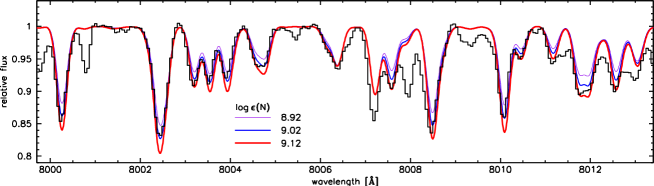
Figure 4.— The 2-0 band of the CN red system in HR 6791. The C and O abundances are set at their best values. The synthetic spectra are calculated for $\log\epsilon(\text{N})=9.02$ and $\pm 0.1\,\text{dex}$.

The CN Red system is also a source of ¹³CN lines and, hence, of the important astrophysical ratio ¹²C/¹³C. Several ¹³CN lines appear unblended with stronger ¹²CN and/or atomic lines and may be used for the isotopic abundance determination after, in some cases, correction for overlying telluric H₂O lines. Figure 5 shows two examples of the synthesis of a key ¹³CN feature.

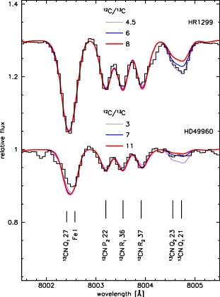
Figure 5.— Part of the 2-0 band of the CN red system in HD 49960 and HR 1299. For each object synthetic spectra calculated with three different carbon isotope ratios are shown.

IV.3. Oxygen

Two O abundance indicators are adopted: the [O i] 6300 Å line and the O i triplet at 7771.9, 7774.2 and 7775.4 Å.

The [O i] line at 6300 Å is blended with a Ni i line (Lambert 1978; Allende Prieto, Lambert, & Asplund 2001) for which we took the $gf$-value from Allende Prieto et al. (2001) and adopted our derived Ni abundance (Table 5). The $\log gf$-value of the [O i] line was set at -9.717 (Allende Prieto et al. 2001). Figure 6 shows the line in HD 18636 with synthetic spectra.

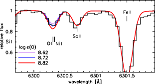
Figure 6.— The [O i] 6300 Å line in HD 18636. Overplotted are synthetic spectra with $\log\epsilon(\text{O})=8.72$ and $\pm 0.1\,\text{dex}$.

The O i triplet lines are sensitive to the adopted effective temperature, and affected by non-LTE effects. The magnitude of the latter effects depends on the atmosphere parameters, the oxygen abundance and differs for each line. For each star, we calculated non-LTE corrections for each line individually with the IDL routine described in Ramírez, Allende Prieto, & Lambert (2007). These non-LTE corrections agree with those from the grid calculated by Fabbian et al. (2009) but cover a more suitable parameter range for our stars. Corrections are largest for 7771.9 Å, the strongest line of the triplet, with the mean correction over the sample being $-0.36\pm 0.07$ dex for the spectroscopic temperatures. For the weakest line (7775.4 Å), the mean correction is on average 0.06 dex smaller. Corrections for the photometric temperature scale are larger by about 0.02 dex. Figure 7 shows observed and synthetic spectra of the oxygen triplet for three wk Gb stars.

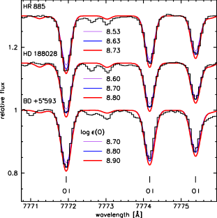
Figure 7.— The O i triplet in three in wk Gb stars. Overplotted are synthetic spectra with O abundances of $\log\epsilon(\text{O})=8.63$ (HR 885), 8.70 (HD 188028), and 8.80 (BD +5^∘593), and spectra with O abundances of $\pm 0.1\,\text{dex}$ for each star. The spectra of HD 188028 and HR 885 are shifted upwards by 0.15 and 0.3.

The oxygen triplet shows a strong temperature sensitivity, while the forbidden 6300 Å line’s temperature dependence is rather moderate. This makes it possible to perform an additional temperature check by finding the effective temperature for each star at which the triplet and the forbidden line give the same O abundance. Interestingly, the derived ‘oxygen’ temperatures - see Figure 8 - suggest that the effective temperatures generally lie between our two determinations.

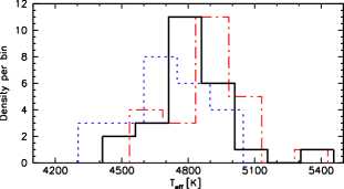
Figure 8.— Histogram of effective temperatures derived spectroscopically (dash-dotted line), photometrically (dotted line), and by comparison of different oxygen lines (thick line). See text for details.

Luck & Heiter (2007) adopted the [O i] 6300 Å as their sole indicator of the O abundance. The $gf$-value of the line was taken from Allende Prieto et al. (2001) with the $gf$-value of the blending Ni i line taken from the experimental determination by Johansson et al. (2003) and the Ni abundance set from the assumption that [Ni/Fe] = 0. This recipe is very similar to ours such that we use Luck & Heiter’s O abundances as the reference for normal GK giants subject to a small systematic difference arising from the use of different model atmosphere grids. The O abundances quoted in Table 4 and discussed in the following sections are therefore the ones derived by the [O i] 6300 Å line.

Table 4Li and CNO abundances of the program stars.

Object	[Fe/H]	Li${}_{\text{NLTE}}$		C		12C/13C	N		O
		sp.	ph.	sp.	ph.		sp.	ph.	sp.	ph.
37 Com	-0.53	1.50	1.16	6.82	6.78	$3.5\pm 0.5$	9.77	10.13	8.72	8.67
BD +5∘593	-0.29	$<$ 0.19	$<$-0.04	6.87	6.77	$3\pm 1$	8.85	8.87	8.80	8.76
HD 18636	-0.16	1.93	1.76	6.91	6.81	$8\pm 2$	9.00	9.02	8.72	8.69
HD 28932	-0.39	2.58	2.27	6.68	6.56	$5\pm 1$	8.87	8.98	8.61	8.56
HD 31869	-0.47	1.06	1.23	6.77	6.75	$4\pm 1$	8.69	8.68	8.47	8.46
HD 40402	-0.14	3.20	3.06	7.25	7.20	$9\pm 2$	8.84	8.86	8.81	8.79
HD 49960	-0.25	0.82	0.55	6.85	6.78	$7\pm 1$	8.98	9.08	8.77	8.73
HD 67728	-0.43	$<$ 0.56	$<$ 0.28	6.81	6.70	$3.5\pm 0.5$	8.66	8.67	8.11	8.08
HD 78146	-0.06	$<$ 1.14	$<$ 0.80	7.29	7.21	$3\pm 0.5$	8.83	8.99	8.77	8.72
HD 82595	0.06	1.42	1.22	7.30	7.21	$3\pm 0.5$	8.86	8.90	8.73	8.69
HD 94956	-0.19	1.21	1.01	6.93	6.84	$5\pm 1$	8.98	9.02	8.71	8.68
HD 120170	-0.51	3.27	3.01	6.57	6.48	$5\pm 2$	8.73	8.79	8.54	8.50
HD 120171	-0.42	$<$-0.27	$<$-0.52	7.53	7.53	$5\pm 1$	8.23	8.22	8.44	8.44
HD 132776	-0.07	1.80	1.41	7.39	7.33	$3.5\pm 0.5$	9.26	9.57	9.07	9.01
HD 146116	-0.39	$<$ 0.17	$<$-0.22	6.73	6.60	$3\pm 0.5$	8.83	9.00	8.49	8.44
HD 188028	-0.18	$<$ 0.19	$<$-0.19	6.70	6.47	$4\pm 1$	8.99	9.09	8.70	8.58
HD 204046	-0.05	$<$ 0.73	$<$ 0.36	7.11	6.97	$3.5\pm 0.5$	8.96	9.09	8.78	8.72
HD 207774	-0.33	$<$ 0.31	$<$ 0.02	7.26	7.16	$3.5\pm 0.5$	8.75	8.79	8.78	8.74
HR 885	-0.35	1.46	1.39	6.48	6.43	$5\pm 1$	8.57	8.56	8.40	8.39
HR 1023	-0.22	3.25	2.91	6.89	6.39	$7\pm 2.5$	9.37	9.41	8.61	8.57
HR 1299	-0.08	2.85	2.78	7.25	7.24	$4.5\pm 0.5$	9.12	9.11	8.62	8.61
HR 6757	-0.08	2.36	1.93	7.18	6.98	$3\pm 0.5$	8.71	8.88	8.80	8.74
HR 6766	-0.18	1.23	1.08	7.01	6.93	$3.5\pm 0.5$	8.70	8.71	8.69	8.67
HR 6791	0.00	1.99	1.82	7.47	7.37	$4\pm 0.5$	9.02	9.00	8.72	8.67
Sun		3.26		8.43		89	7.83		8.69

Note. — Abundances of element A are given in $\log\epsilon(\text{A})$. Solar abundances are taken from Asplund et al. (2009). The errors for the different abundances take into account the effect of uncertain parameters on the abundances and difficulties in the synthesis of the lines, such as continuum placement and quality of the spectra. These errors are added in quadrature. For N additionally the C error is added, since the only abundance indicator - the CN red system - includes C. We estimate errors of $\sigma_{\text{C}}=0.25$, $\sigma_{\text{N}}=0.3$, $\sigma_{\text{O}}=0.11$, and $\sigma_{\text{Li}}=0.25$.

HD 120171

The star HD 120171 shows a high C abundance compared to the rest of the program stars. The low carbon deficiency is accompanied by an only moderate N overabundance and normal O abundance. Overall this object does not show the striking characteristics of a wk Gb stars and might rather be considered normal or intermediate between the normal giants and the wk Gb stars.

IV.4. Lithium

Only one Li feature is prominent in our spectra, the 6708 Å  Li i resonance doublet. We determine the Li abundance by synthesizing the feature and an Fe i line at $6707.44\,\AA$. The data used for the wavelength positions and ${\log gf}$ values for ⁷Li and ⁶Li components of this feature are taken from Lambert & Sawyer (1984). We include CN blends in our synthesis and use the C and N abundances derived as described in sections IV.1 and IV.2. The precision of the Li abundance determination depends on the strength of the lines. For weak lines a change of $\pm 0.05$ in the log already leads to recognizable differences, while for strong lines sometimes a change of $\pm 0.2$ is necessary (see Figure 9 for an example of Li lines with different strength; the Li i line strength varies significantly even though all three stars have comparable temperatures). Apart from the uncertainty from the synthesis of the lines, the error for the Li abundances due to uncertainties of the model atmosphere parameters is not likely to exceed 0.2 dex. The biggest impact comes from an uncertain temperature. A change in ${T_{\text{eff}}}$ of $\pm 200\,\text{K}$ leads to a change of 0.23 dex in the Li abundance. Both ${\log g}$ and ${v_{t}}$ have only a minor influence on the determined Li abundances. A determination of the ⁷Li/ ⁶Li isotope ratio is unpromising. For large Li abundances the doublet blends with the close-by Fe i line. The 6708 Å  Li i line can be affected by non-LTE effects which can lead to positive or negative abundance corrections. The size of the corrections depends on the stellar parameters and the lithium abundance itself (Lind, Asplund, & Barklem 2009). We calculated NLTE corrections suitable for the parameters and Li abundances of the program stars by interpolating between the tabulated values of Lind et al. (2009).

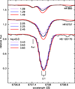
Figure 9.— Spectra of three wk Gb stars and overplotted synthetic spectra. The synthetic spectra are calculated with Li abundances of $\log\epsilon(\text{Li})=1.29$ (HR 885), 2.25 (HR 6757), and 3.63 (HD 120170). Additional spectra with $\pm 0.2\,\text{dex}$ are also shown for each star.

The corrected Li abundances cover a wide range as can be seen in Table 4.

Figure 10 shows a comparison of our determined Li abundances with the values Palacios et al. (2012) and Lambert & Sawyer (1984). Differences between the two literature sources are naturally small, since both are using the same equivalent widths of the Li lines. Our newly determined Li abundances in general agree well with the literature data. A larger scatter can be recognized at lower Li abundances, mainly due to the more difficult detection and analysis of these Li lines, which only allows the determination of upper limits.

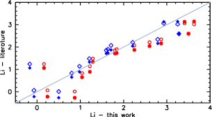
Figure 10.— Comparison of Li LTE abundances with literature values. Circles represent the comparison of our spectroscopic results with Palacios et al. 2012 (filled) and the various results presented in Lambert & Sawyer 1984 (open). Analogously, squares indicate the comparison of our photometric results.

IV.5. Other elements

Abundances for Na, Mg, Al, Si, Ca, Ti, Cr, Fe, Ni, Y, and Eu were determined. Most of these elements appear in the spectra with a sufficient number of unblended lines. Their abundances can be derived by force-fitting the abundances of the lines to match measured equivalent widths as described in Sect. III. The atomic data for all lines used in the analysis is taken from Luck & Heiter (2007). We attempted to perform our analysis as similar as possible to Luck & Heiter’s and to utilize as many of their lines as possible. Not all of the lines were present in our objects but no additional lines from other sources were added. We determine solar abundances for each of the lines used and derive relative abundances for the elements in the wk Gb stars on a per-line basis.

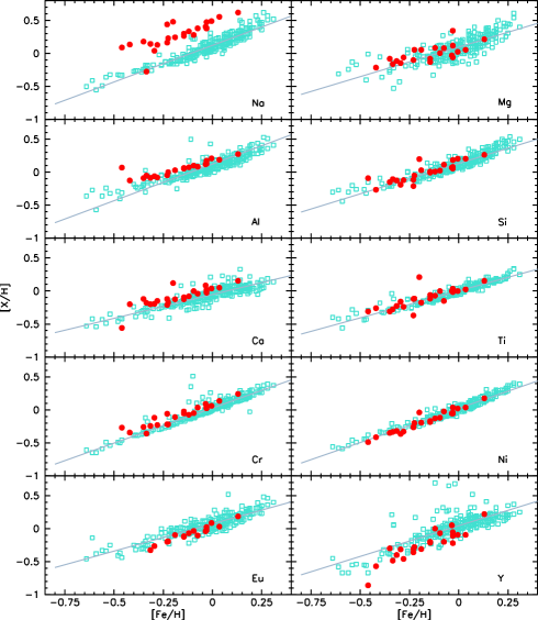
Figure 11.— Trends of element abundances vs. metallicity in the wk Gb stars for spectroscopic temperatures (filled circles), compared to giants from Luck & Heiter 2007 (open squares). The solid lines indicate the slopes of the trends from the spectroscopic analysis of Luck & Heiter (2007).

Na

We measured equivalent widths of Na i lines at 6154.225 and 6160.747 Å in our spectra.

The Na abundance is enhanced in the wk Gb stars with $[\text{Na/Fe}]=0.46\pm 0.12$ for the spectroscopic temperatures and $[\text{Na/Fe}]=0.37\pm 0.13$ for the photometric temperatures. We determined a [Na/Ca] ratio of $0.34\pm 0.15$ (sp.) and $0.37\pm 0.20$ (ph.). Drake & Lambert (1994) determined $[\text{Na/Ca}]=0.16$ for a smaller sample of the wk Gb stars. A direct comparison with their result, however, is not easily possible since their abundance data was derived relative to Pollux. For the objects that both samples have in common the EW that we measured for the Na lines are in excellent agreement with the ones measured by Drake & Lambert (1994). The mean differences are $-1.9\pm 5.95\,\text{m\AA}$ for the 6154 Å line and $1.57\pm 10.78\,\text{m\AA}$ for the 6160 Å line. The differences in the Na abundances between our and Drake & Lambert’s analysis then depend on the differences in model parameters and the reference to Pollux.

The comparison with the abundances from Luck & Heiter (2007) shows a significant enhancement of Na in the wk Gb stars compared to the normal giants by about 0.3 dex (see Figure 11). Note also that the only star that shows a Na comparable with the data from Luck & Heiter (2007) is HD 120171, whose C and N abundance are closest to those of normal giants. A significant enrichment of Na in the rest of the wk Gb stars could be a result of a large amount of ²²Ne converted to ²³Na.

Mg, Al, Ca, Si, Ti, Cr, Ni, Eu, and Y

We determined the abundances of a group of additional elements, including the $\alpha$-elements Mg, Ca, Si, and Ti, the $r$-process element Eu and the $s$-process element Y, using again the line data from Luck & Heiter (2007). In Figure 11 we compare these abundances with the abundances from Luck & Heiter (2007). Contrary to Na (see above) the abundances of the elements from Mg to Y in the wk Gb stars are consistent with the ones for the normal giants from Luck & Heiter (2007).

The abundance trends of the elements found for the wk Gb stars (except Na) supports the conclusion that wk Gb stars are normal in all other respects than their CNO-cycle element and Li abundances.

V. Discussion

V.1. Preliminary remarks

Compositions of wk Gb stars will be compared and contrasted with results for nearby normal GK giants presented by Luck & Heiter (2007) whose abundance analysis closely resembles ours, particularly with respect to selection of lines and atomic/molecular data. It seems apparent, as noted above, that the wk Gb stars have experienced substantial exposure to the H-burning CN-cycle. After a few preliminaries, it is this aspect which we discuss in the next section.

One of the preliminary remarks concerns the [Fe/H] distributions of our and Luck & Heiter’s sample. These are compared in Figure 12 and show that the wk Gb stars have a higher proportion of low [Fe/H] stars (say, [Fe/H] $<-0.2$) than do the nearby giants which Luck & Heiter show have the same distribution as the nearby dwarfs (Luck & Heiter 2006) with both giant and dwarf distributions having mean values [Fe/H] $\simeq 0.00$. In contrast, the wk Gb sample has a mean value $[\text{Fe/H}]=-0.23$. Unless the search for wk Gb stars was concentrated more heavily on metal-poor giants, this result implies that production of wk Gb stars is more readily accomplished among metal-poor stars.

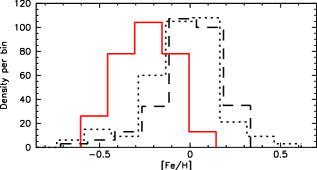
Figure 12.— Metallicity distribution in the wk Gb stars (solid line) compared to the [Fe/H] distributions from the giants sample in Luck & Heiter (2007) (dashed line) and the dwarf sample from Luck & Heiter (2006) (dotted line). The distributions for the wk Gb stars and the dwarf data were scaled to the number of giants from Luck & Heiter (2007).

A second preliminary remark concerns the stellar masses. The normal giants run from about 1 $M_{\odot}$ to about 3 $M_{\odot}$ with the majority of stars falling between 1 and 2 $M_{\odot}$ (Luck & Heiter 2007). In contrast, the trigonometrical parallaxes and effective temperatures place the masses of our wk Gb sample (see above) between 2.5 $M_{\odot}$ and about 5 $M_{\odot}$, i.e., our stars are what are usually referred to as intermediate mass stars and the nearby stars are low mass stars. This mass difference translates to differences in the evolution of the stars, e.g., low mass but not intermediate mass stars experience a He-core flash. But a more significant difference may be the differing distributions of rotational velocity. As Kraft (1967) showed, the mean rotational velocity declines from high values on the upper upper main sequence stars ($M>1.25\,M_{\odot}$) to low values on the lower main sequence. Thus, the wk Gb stars may have left the main sequence as rapid rotators but the majority of Luck & Heiter’s sample of giants departed the main sequence as slow rotators. If rapid rotation of an intermediate mass star is responsible for the creation of a wk Gb star, one may wonder why such a small minority of intermediate mass main sequence stars evolve to wk G stars.

The third preliminary remark concerns the signatures of the H-burning, by the CN-cycle and possibly the ON-cycles. All normal giant stars are expected to have experienced the first dredge-up which brought mildly CN-cycled material into their atmosphere. Low mass stars may have also experienced additional mixing at the luminosity bump on the red giant branch or, perhaps, at the He-core flash. Luck & Heiter’s sample includes stars on the red giant branch (pre-He-core flash) and stars at the red clump (post-He-core flash). Intermediate mass giants experience first and second dredge-up but not the He-core flash.

Signatures of the addition of mildly CN-cycled material to an atmosphere include a slight reduction of ¹²C, increase of ¹³C, increase of ¹⁴N with the constraint that the sum ¹²C+¹³C+¹⁴N is conserved. In the first dredge-up for low mass stars, the ¹⁶O abundance is not changed measurably. Changes of the ¹⁷O and ¹⁸O abundance are expected. It is unfortunate that these two heavier O isotopes are not accessible from optical spectra. In the absence of production by the Cameron-Fowler mechanism, the atmosphere’s Li abundance will be lowered severely.

These predictions are confirmed by Luck & Heiter’s sample, as they noted. In particular, comparison of results for nearby dwarfs and giants showed C in the giants was lowered by about 0.2 dex, N was increased in giants over levels seen in dwarfs such that the C+N sum was conserved, and O abundances among dwarfs and giants were similar. (The spectral coverage did not allow Luck & Heiter to determine the carbon isotopic ratio but results in the literature show that the ratio is lowered in giants in qualitative, if not quantitative, agreement with expectation.)

Carbon and nitrogen abundances for wk Gb and normal giants are compared in Figure 13 with the left-hand panel presenting our results and the right-hand panel showing results for nearby normal giants from Luck & Heiter (2007).

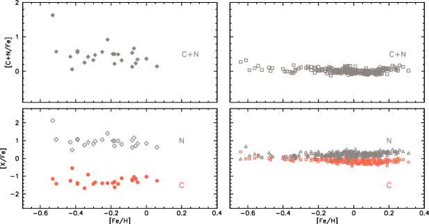
Figure 13.— Lower left panel: Spectroscopically derived abundances of C (filled circles) and N (open squares) for the wk Gb stars. Lower right panel C (open squares) and N (open triangles) data from Luck & Heiter (2007). Upper left panel: Sum of C and N abundances in the wk Gb stars. Upper right panel: The same for the giants from Luck & Heiter (2007). For this plot we use the solar abundances for C and N as derived by Luck & Heiter (2007) with the newest MARCS models: $\log\,\epsilon(\text{C})=8.50$, $\log\,\epsilon(\text{N})=8.18$.

A direct way to examine the assertion that the wk Gb stars are unusually rich in CN-cycled material is to plot in Figure 13 the C and N abundances versus [Fe/H] for the wk Gb stars (left-hand lower panel) and normal nearby giants (right-hand lower panel). The contrast between the two samples is striking: the wk Gb stars are about a factor of 20 underabundant in C relative to normal giants. Additionally the sum of C and N (here C is the sum of ¹²C and ¹³C) is about 0.3 dex greater on average for wk Gb stars than for the nearby giants over a common range in [Fe/H]. A possible explanation for this difference is that, in addition to excessive CN-cycling, some ¹⁶O has been processed to ¹⁴N through partial ON-cycling. The fact that the ¹²C/¹³C ratios are very low is also evidence for CN-cycling.

In terms of the C and N abundances, there appears a clean distinction between normal and wk Gb giants. This, however, may be an artefact because the discovery of wk Gb stars has come almost entirely from visual inspection of low dispersion spectra. The star with a seemingly intermediate C abundance is HD 120171 (see section IV.3).

Lithium in normal giants is generally severely depleted, as predicted because the giant’s convective envelope dilutes the lithium that has survived in the main sequence star, the giant’s progenitor. This dilution is illustrated in the right-hand panel of Figure 14 where Li abundances for Luck & Heiter’s giants are contrasted with Li abundances for dwarfs from Lambert & Reddy (2004). The non-LTE Li abundances for wk Gb stars (Table 4) span the range from the interstellar abundance ($\log\epsilon(\text{Li})\simeq 3.3)$, the star’s likely initial Li abundance, to severely depleted abundances (see also left-hand panel of Figure 14 for a comparison of wk Gb LTE abundances with normal giants and dwarfs). The most direct interpretations of this 1000-fold minimum spread in Li abundances is that Li dilution by the giant’s convective envelope is in some cases offset by internal synthesis of Li to an extent that varies greatly from star-to-star despite comparable degrees of contamination by CN-cycle products.

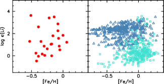
Figure 14.— Spectroscopic LTE Li abundances of wk Gb stars (left panel) compared to giants from Luck & Heiter (2007) (squares, right panel) and dwarf data from Lambert & Reddy (2004) (triangles, right panel).

V.2. Clues from nucleosynthesis

To unravel the links between the composition of wk Gb stars and their origins calls for – first – dissection of the nuclear processes to which their atmospheres has been exposed and – second – identification of the mechanism responsible for transport of the products of these nuclear processes from their site of operation to the stellar atmosphere.

A high N/C ratio and a low ¹²C/¹³C ratio are the principal signatures that H-burning CN-cycle products now contaminate a wk Gb star’s atmosphere. In parallel with the CN-cycle, the slower ON-cycles and the NeNa- and MgAl-chains may run with observable consequences. Finally, lithium production by the Cameron & Fowler (1971) mechanism converts available ³He via ⁷Be to ⁷Li. Since the atmospheric Li abundance depends greatly on the efficiency of transfer of the ⁷Be and ⁷Li to low temperatures in order to avoid destruction by protons, prediction of a wk Gb star’s Li abundance is fraught with uncertainty.

Given that the ³He reservoir is potentially capable of synthesizing Li to levels far greater than are observed in wk Gb stars, it is intriguing that the maximum observed Li abundance is coincident with the interstellar Li abundance - see Lambert & Sawyer (1984) for a speculative interpretation of this fact. Lithium in the rare examples of Li-rich (normal) giants can exceed the interstellar abundance by a factor of several (Charbonnel & Balachandran 2000; Kumar, Reddy, & Lambert 2011). Thus, little weight should be given the above coincidence.

In contrast to the case of lithium, the relative abundances from the H-burning cycles and chains are predictable with fair certainty from nucleosynthetic arguments, even if aspects of the stellar evolutionary context remain murky.

Consumption of protons by the (slow) CN-cycle converts four protons to an $\alpha$-particle and, after a few cycles, establishes equilibrium abundances of the participating nuclides: ¹²C, ¹³C, ¹⁴N and ¹⁵N with broadly ¹²C/¹³C $\sim 3$, ¹⁴N/¹²C $\sim$ 100, and ¹⁴N/¹⁵N $>$ 20,000 at the temperatures of efficient H-burning. Before presenting a semi-quantitative interpretation of the wk Gb star CNO abundances, one may note that the abundances (Table 4) mirror the above estimates: the N/C ratio is about 100, and the carbon isotopic ratio is 3-4 for many stars.

Two boundary prerequisites for the preeminence of the CN-cycle must be recognized. First, the CN-cycle is in competition for protons with the $pp$-chains. Second, the ON-cycles process protons more slowly than the CN-cycle and, thus, there is a possibility that the CN-cycle and the $pp$-chain will complete the conversion of H to He before the ON-cycles will have had time to imprint their effect on the CNO abundances.

Our evaluation of these two conditions is made for a typical wk Gb star with [Fe/H] $\sim-0.3$ and initial CNO abundances (i.e., in the progenitor dwarf) of approximately C = 8.2, N = 7.5 and O = 8.6 . Nuclear reaction rates are taken from the NACRE compilation (Angulo et al. 1999); recent updates (Adelberger et al. 2011) are unimportant for what follows.

The relative efficiencies of the $pp$-chains and the CN-cycle in consuming protons are set by the slowest rate for each process: $p(p,e^{+}\nu_{e})d$ for the $pp$-chain and ¹⁴N($p,\gamma)^{15}$O for the CN-cycle. As is well known, the $pp$-chains are the principal consumer of protons at ‘low’ temperatures and the CN-cycle at ‘high’ temperatures. For N = 7.8, the consumption rates are equal at about 20 million degrees. Thanks to the Coulomb barrier between the ¹⁴N and the proton, the $pp$-chain rapidly outperforms the CN-cycle as the temperature is lowered below 20 million degrees; for example, the $pp$-chain is favored by a factor of $10^{5}$ at 10 million degrees. Thus, the CN-cycled material present in a wk Gb star was processed at temperatures of 20 million degrees or hotter.

The ON-cycles consume protons more slowly than the CN-cycle and are unlikely to achieve their equilibrium abundances. Flow through the ON-cycles is controlled by the ratio of the reaction rates ¹⁵N$(p,\alpha)^{12}$C which closes the CN-cycle and ¹⁵N$(p,\gamma)^{16}$O which opens the ON-cycles. This ratio reflecting the relative strengths of the strong to the electromagnetic interaction favors closure of the CN-cycle by a factor of about 1000. However, in advance of the ON-cycles reaching equilibrium, some ¹⁶O is converted to ¹⁴N via ¹⁷O. The temperature-dependent CN-cycle equilibrium ratio for N/C may be increased by N from O consumption as ¹⁶O is processed to ¹⁴N ahead of equilibrium within the ON-cycles.

Given this contrast between the times for completion of the CN- and ON-cycles, one may note two reasons for expecting the CN-cycle products in a wk Gb stellar atmosphere not to be accompanied by ON-cycle equilibrium products which are ¹⁶O-poor and ¹⁴N-rich. First, the episode of H-burning may not be active for the length of time required to run the ON-cycle yet able to run the CN-cycle to equilibrium. Second, protons may be totally consumed by the CN-cycle before the ON-cycle achieves equilibrium. For example, for our typical wk Gb star with C+N = 8.3 and H/C = 3.7 and four protons consumed per CN-cycle, 1200 (=$10^{3.7}-10^{0.6}$) cycles exhaust the proton supply which would indicate that the ON-cycle being a factor of 1000 slower than the CN-cycle will be largely idle. (At much lower metallicities when the number of C+N catalysts is lower, the CN-cycle must run more cycles to exhaust the protons and, then, O-poor (and C-poor) but very N-rich stars may be anticipated.) A corollary deserves comment. If the ON-cycle has operated in the material mixed into the atmosphere, the atmosphere will become H-poor and He-rich but the wk Gb stars are obviously not extremely He-rich. An accurate determination of their He/H ratio is an elusive goal.

Now consider the typical wk Gb star with initial abundances C = 8.2, N = 7.5, and O= 8.6 or N/C = -0.7 and N/O = -1.1. Suppose the atmosphere is mixed with a large amount of CN-cycled material, the atmospheric composition tends to equilibrium abundances of the cycle. Then, the N/C becomes 2.1, 1.9 and 1.6 for temperatures T₆ = 20, 30 and 50, respectively, with N/O = $-0.3$ for these temperatures. In Figure 15, we show N/O versus N/C. With the exceptions of 37 Com and HR 1023 having high N/C and N/O, and HD 120171 with its high C and low N abundances, the wk Gb stars fall in a slanted rectangle centered on about N/O $\simeq 0.3$ and N/C $\simeq 2$. The predicted N/Cs cross the slanted rectangle but the N/O ratio does not: N/O = $-0.3$ is predicted but the stars span the range 0.0 to $+$0.6. One way to raise the N/O ratio is to assume that the ON-cycles have partially converted ¹⁶O to ¹⁴N in the run up to the never attained condition of ON-cycle equilibrium. Suppose that at T₆ = 30 the O abundance was depleted from 8.6 to 8.4, then N/O = 0.2 and N/C = 2.2 which combination falls within the rectangle (open circle in Figure 15).

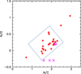
Figure 15.— N/O vs. N/C for the wk Gb stars (filled circles). Predicted N/C and N/O ratios are marked with crosses. The N/O ratio derived by partial conversion of ¹⁶O to ¹⁴N is marked with an open circle. See text for details.

There is evidence for a star-to-star variation in O depletion. In Figure 16, we compare [O/Fe] for wk Gb stars and normal giants with a line corresponding to a fit to the latter results. If O depletion is the explanation for the N/O discrepancy, there will be a correlation between the O deficiency as shown in Figure 16 by the amount that [O/Fe] falls below the line defined by the normal giants (say, $\Delta$[O/Fe]) and the N/O ratio. Figure 17 shows the $\Delta$[O/Fe] versus N/O relation with the majority of points exhibiting a loose correlation of the expected sign. There are four outliers: 37 Com, HR 1023, HD 132776 with high N abundances and HD 120171 with a low O abundance but not the anticipated N overabundance. HD 67728 with a large negative $\Delta$[O/Fe] ($-0.6$) may also be an outlier.

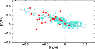
Figure 16.— Spectroscopic abundance of oxygen vs. iron abundance in the wk Gb stars (filled circles) compared to the oxygen abundance of normal giants (open squares, Luck & Heiter 2007). The grey line is a linear fit to the normal giants oxygen abundances.

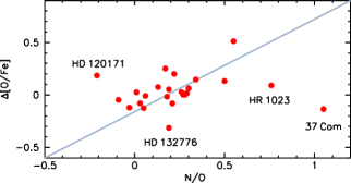
Figure 17.— $\Delta$[O/Fe] versus N/O for the wk Gb stars. The grey line indicates an assumed linear correlation and is not a fit to the data points. Objects with peculiar values are labeled and explained in the text.

If the CN-cycle supplemented by partial operation of the ON-cycles has occurred, a sum rule operates, i.e., the sum of initial C, N, and O nuclei is conserved. This rule may be checked using the nearby giants to define the initial sum. Figure 18 shows the CNO sum versus [Fe/H] for wk Gb stars and the nearby giants. Apart from two outliers among the wk Gb stars (37 Com and HR 1023 ), the sum for the wk Gb stars may be somewhat systematically greater than for the nearby giants; the upper envelope for the wk Gb stars is approximately 0.1 dex greater than for nearby giants of a similar metallicity. Perhaps, Figure 18 gives an impression that the CNO sums for some wk Gb stars maybe greater than for nearby giants. This is contrary to expectation for contamination of wk Gb atmospheres by CNO-cycled material, casts doubt on the proposal that ON-cycled material is present in some wk Gb stellar atmospheres, and directs suspicion to systematic effects in the abundance analysis. This suspicion should likely be directed at the C abundances which were derived from different spectral signature for the two samples (see Section 4.1): the CH G-band for wk Gb stars and C i lines and a C₂ feature for nearby giants. A systematic error in the derived C abundance translates to an error in the N abundance obtained from CN lines and, thence, into the CNO sum. A change of the CN dissociation energy by 0.05 eV (see section IV.2) would result in a change of $<0.1$ in the CNO sum.

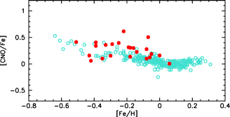
Figure 18.— Sum of C, N, and O abundances in the weak Gb stars (filled circles) compared to the giants from Luck & Heiter (2007) (open circles). For this plot we use the solar abundances for C, N, and O as derived by Luck & Heiter (2007) with the newest MARCS models: $\log\,\epsilon(\text{C})=8.50$, $\log\,\epsilon(\text{N})=8.18$, and $\log\,\epsilon(\text{O})=8.81$.

Other H-burning processes occur in parallel with the CN-cycle and redistribution of the relevant catalysts may lead to observable abundance anomalies. The following discussion is based on the NACRE rates (see Arnould, Goriely, & Jorissen 1999). The NeNa chain provides a redistribution of Ne isotopes and an increase of the Na abundance and the MgAl chain offers the possibility of changing the relative abundance of the three stable Mg isotopes: ²⁴Mg, ²⁵Mg, and ²⁶Mg. Unfortunately, Ne and its isotopes are not observable in K giants but Na (see above) is observable. Arnould et al. show that in a solar mix Na increases by about a factor of four from running of the ²²Ne($p,\gamma)^{23}$Na reaction over the temperature range and proton consumptions levels required for efficient CN-cycling. Such a quantitative estimate of the Na increase is dependent on several uncertain reaction rates in the NeNa chain. The increase for a wk Gb star depends on the intrinsic ²²Ne vs [Fe/H] and [Na/H] vs [Fe/H] relations. Figure 11 shows that indeed the wk Gb stars are Na-rich relative to the normal nearby giants. This increase results from the NeNa chain operating in parallel with the CNO-cycles. The MgAl chain can lead to the increase of ²⁶Mg and a decrease of ²⁵Mg relative to the dominant isotope ²⁴Mg. These alterations demand very deep mixing (i.e., hotter temperatures than for activation of the NeNa chain) and a considerable conversion of H to He before significant alteration of the Mg isotopic abundances. The inspection of our spectra indicates that MgH lines are present in the wk Gb stars. Since the C₂ Swan lines that are often blended with key MgH lines are not present in the wk Gb stars, an isotopic abundance determination is promising and will be a future investigation.

VI. Concluding remarks

Our abundance analysis of a complete sample of known northern wk Gb stars allows the illustration of new and comprehensive results about their atmospheric composition including several results which contradict published conclusions, often based on abundances for smaller samples of wk Gb stars. The new results show that the atmospheres are seriously contaminated with products of the H-burning CN-cycle and associated processes. Speculations about episodes in the evolution of these stars which result in the demarcation of wk Gb stars from normal giants are here curtailed. These concluding remarks are limited to setting the stage on which the key distinguishing episode in stellar evolution must play. Qualitative and certainly quantitative theoretical exploration of potential episodes are left to others.

A boundary condition generally accepted but not proven decisively from observations is that the striking composition of a wk Gb star results from upheavals internal to the star and is not imposed by mass transfer from or induced by an orbiting companion star (Tomkin, Sneden, & Cottrell 1984; Griffin 1992). The binary fraction among wk Gb stars is thought to be normal in sharp contrast, for example, to the Ba II K giants where all stars are binaries and the peculiar giant was created by transfer of $s$-process enriched material from its companion when it was an AGB star (McClure 1983). A comprehensive radial velocity survey of wk Gb stars for orbital variations has yet to be undertaken. Two stars – HR 1023 and HR 6791 – are known to be spectroscopic binaries (Lucke & Mayor 1982; Tomkin et al. 1984; Griffin 1992).

The wk Gb stars are systematically metal-poor relative to local field giants (Figure 12). This result shown here for the first time may possibly be, in part, a selection effect.

An important boundary condition is that the masses of wk Gb stars (2.5-5$M_{\odot}$) are substantially greater than the masses of typical giants in the local field. This result, first shown by Palacios et al. (2012), arises from the rereduction of the Hipparcos parallaxes (van Leeuwen 2007). This difference in mass encourages the speculation (discussed above in Sect. V.1) that rotationally-induced mixing in the main sequence progenitor may be the root cause of the abundance anomalies of the wk Gb stars. Lower mass stars are rotationally-braked before reaching the main sequence and observations show experience the mild effects of the standard first- dredge up, which salts a low mass giant’s atmosphere to a minor but observable degree with CN-cycled material, as discussed by, for example, Luck & Heiter (2007).

At the masses of the wk Gb stars, rapidly-rotating main sequence stars are common and rotational braking not a guaranteed phenomenon. Thus, one may speculate that particular combinations of initial internal distribution of angular rotation rates, rotationally-induced mixing and rotational braking may lead to the severe contamination of the stellar interior by CN-cycled material. The parameters for suitable combinations must be fairly stringent or the wk Gb phenomenon would be the norm and not a peculiar condition for G-K giants. There is also a suspicion that the wk Gb giants are a class apart with an unpopulated gap separating them from normal giants. This, if true for giants of the same mass as the wk Gb stars, presumably translates to special constraints on origins for wk Gb stars invoking rotation.

In order to examine the ‘rotation’ solution in more detail in advance of theoretical advances, further observational investigation may be proposed. Three are sketched here.

First, a comprehensive abundance analysis needs to be undertaken for a large sample of stars at the masses of the wk Gb stars on the main sequence and, in particular in the Hertzsprung gap. Do wk Gb stars make an appearance on the main sequence or in the gap before becoming giants? Note that, if the spectroscopic temperatures are adopted, most of the wk Gb stars are in fact on the red side of the gap (Figure 2).

Second, there are several ways in which the present abundance analysis could be improved or extended, apart from the obvious extension to wk Gb stars in the southern hemisphere beyond the grasp of a Texas telescope. It is possible with due care given to correction for telluric lines to obtain accurate measurements of C i lines in the red (see above). In addition, infrared spectra at 2.3 microns will provide measurements of the CO first-overtone bands which will yield a different measure of the C abundance and, hence a check on the suggestion that N has been augmented by partial ON-cycle conversion of some ¹⁶O to N. A more difficult observation would involve spectra at 4.6 microns and a search for the isotopes ¹⁶O and ¹⁷O.

Third, the search for wk Gb stars should be expanded. One key question concerns the apparent clean distinction between normal and wk Gb giants - do stars with intermediate C (and other) abundances exist in detectable numbers? Is the wk Gb star phenomenon limited to particular metallicities?

Table 5Element abundances of the program stars with respect to H.

Object	Na		Mg		Al		Si		Ca		Ti		Cr		Fe		Ni		Y		Eu
	sp.	ph.	sp.	ph.	sp.	ph.	sp.	ph.	sp.	ph.	sp.	ph.	sp.	ph.	sp.	ph.	sp.	ph.	sp.	ph.	sp.	ph.
37 Com	0.09	-0.11			0.07	-0.11	-0.09	0.05	-0.56	-0.82	-0.31	-0.67	-0.27	-0.57	-0.46	-0.50	-0.49	-0.54	-0.86	-1.15
BD +5∘593	0.17	-0.02	-0.10	-0.20	-0.05	-0.18	-0.12	-0.07	-0.12	-0.32	-0.12	-0.38	-0.22	-0.38	-0.23	-0.35	-0.27	-0.38	-0.31	-0.42	-0.20	-0.18
HD 18636	0.28	0.17	0.01	-0.07	0.10	0.01	0.03	0.06	0.00	-0.14	0.00	-0.20	-0.05	-0.17	-0.10	-0.17	-0.12	-0.21	-0.07	-0.15	-0.04	-0.02
HD 28932	0.04	-0.16	-0.15	-0.25	-0.06	-0.23	-0.19	-0.14	-0.20	-0.44	-0.16	-0.44	-0.12	-0.32	-0.30	-0.40	-0.37	-0.46	-0.32	-0.45	-0.27	-0.25
HD 31869	0.13	0.09	-0.06	-0.08	-0.08	-0.11	-0.12	-0.12	-0.15	-0.19	-0.24	-0.29	-0.23	-0.27	-0.28	-0.31	-0.33	-0.35	-0.46	-0.48
HD 40402	0.38	0.27	-0.06	-0.11	0.13	0.04	0.06	0.11	-0.03	-0.16	0.00	-0.16	0.03	-0.10	-0.03	-0.08	-0.06	-0.10	-0.22	-0.33
HD 49960	0.25	0.19	0.06	0.03	0.03	-0.02	0.03	0.05	-0.13	-0.20	-0.18	-0.27	-0.11	-0.16	-0.19	-0.22	-0.20	-0.22	-0.31	-0.35	-0.10	-0.10
HD 67728	0.44	0.30					-0.21	-0.20	-0.21	-0.38	-0.37	-0.51	-0.06	-0.18	-0.23	-0.31	-0.26	-0.39	-0.36	-0.57
HD 78146	0.38	0.20	0.08	0.02	0.09	-0.09	0.12	0.25	-0.04	-0.28	-0.15	-0.46	0.04	-0.16	-0.08	-0.08	-0.03	-0.04	-0.20	-0.32	-0.11	-0.08
HD 82595	0.62	0.49	0.22	0.15	0.28	0.17	0.27	0.31	0.16	0.01	0.16	-0.04	0.24	0.10	0.13	0.08	0.18	0.12	0.22	0.19	0.19	0.20
HD 94956	0.27	0.13	-0.13	-0.21	0.06	-0.07	0.01	0.07	-0.13	-0.30	-0.12	-0.32	-0.03	-0.13	-0.15	-0.22	-0.19	-0.26	-0.20	-0.29	-0.13	-0.11
HD 120170	0.14	-0.03	-0.22	-0.31	-0.13	-0.26	-0.27	-0.24	-0.20	-0.39	-0.26	-0.51	-0.35	-0.50	-0.42	-0.51	-0.42	-0.52	-0.57	-0.67
HD 120171	-0.28	-0.29	-0.16	-0.17	-0.05	-0.07	-0.11	-0.10	-0.18	-0.20	-0.28	-0.31	-0.36	-0.38	-0.34	-0.34	-0.34	-0.35	-0.49	-0.50
HD 132776	0.48	0.30	0.12	0.08	0.18	0.01	0.19	0.33	-0.10	-0.24	0.04	-0.27	0.05	-0.13	-0.03	-0.02	0.04	0.05	-0.11	-0.23	-0.02	0.01
HD 146116	0.15	-0.10	-0.12	-0.24	-0.09	-0.29	-0.13	-0.03	-0.20	-0.48	-0.23	-0.57	-0.25	-0.48	-0.32	-0.41	-0.32	-0.41	-0.40	-0.55	-0.33	-0.29
HD 188028	0.34	0.08	0.09	-0.04	0.08	-0.14	0.01	0.14	-0.08	-0.38	-0.07	-0.48	-0.08	-0.37	-0.12	-0.23	-0.13	-0.22	0.00	-0.05	-0.07	-0.03
HD 204046	0.38	0.14	0.35	0.23	0.16	-0.05	0.08	0.18	0.02	-0.26	-0.02	-0.39	0.03	-0.24	-0.03	-0.11	-0.04	-0.12	-0.06	-0.21	0.02	0.05
HD 207774	0.23	0.04	0.05	-0.07	0.00	-0.08	-0.05	0.02	-0.17	-0.40	-0.12	-0.43	-0.22	-0.42	-0.23	-0.33	-0.20	-0.31	-0.28	-0.32	-0.19	-0.17
HR 885	0.18	0.14	-0.08	-0.11	-0.09	-0.13	-0.15	-0.14	-0.12	-0.17	-0.31	-0.39	-0.26	-0.29	-0.35	-0.38	-0.35	-0.39	-0.30	-0.28		-0.28
HR 1023	0.48	0.28					0.20	0.10	0.12	-0.14	0.21	-0.16			-0.20	-0.41	-0.04	-0.29
HR 1299	0.49	0.45	0.03	0.01	0.21	0.18	0.21	0.23	0.04	0.00	0.00	-0.06	0.06	0.02	-0.01	-0.02	0.02	0.02	-0.10	-0.12	0.09	0.08
HR 6757	0.41	0.12	-0.03	-0.16	0.12	-0.13	0.07	0.22	0.09	-0.26	0.00	-0.46	0.09	-0.21	-0.04	-0.13	-0.06	-0.18	0.05	-0.14	-0.04	0.00
HR 6766	0.30	0.19	-0.08	-0.14	0.07	-0.03	-0.01	0.03	-0.10	-0.24	-0.06	-0.23	-0.06	-0.16	-0.15	-0.21	-0.17	-0.23	-0.22	-0.29	-0.12	-0.10
HR 6791	0.56	0.50	0.06	0.01	0.19	0.13	0.21	0.21	0.05	-0.03	0.03	-0.06	0.14	0.13	0.04	0.00	0.04	-0.01	-0.10	-0.25	0.03	0.04

References

- Adelberger, García, Robertson, Snover, Balantekin, Heeger, Ramsey-Musolf, Bemmerer, Junghans, Bertulani, Chen, Costantini, Prati, Couder, Uberseder, Wiescher, Cyburt, Davids, Freedman, Gai, Gazit, Gialanella, Imbriani, Greife, Hass, Haxton, Itahashi, Kubodera, Langanke, Leitner, Leitner, Vetter, Winslow, Marcucci, Motobayashi, Mukhamedzhanov, Tribble, Nollett, Nunes, Park, Parker, Schiavilla, Simpson, Spitaleri, Strieder, Trautvetter, Suemmerer, & Typel (2011) Adelberger, E. G., García, A., Robertson, R. G. H., et al. 2011, Reviews of Modern Physics, 83, 195
- Allende Prieto, Lambert, & Asplund (2001) Allende Prieto, C., Lambert, D. L., & Asplund, M. 2001, ApJ, 556, L63
- Allende Prieto, Lambert, & Asplund (2002) —. 2002, ApJ, 573, L137
- Alonso, Arribas, & Martínez-Roger (1999) Alonso, A., Arribas, S., & Martínez-Roger, C. 1999, A&AS, 140, 261
- Angulo, Arnould, Rayet, Descouvemont, Baye, Leclercq-Willain, Coc, Barhoumi, Aguer, Rolfs, Kunz, Hammer, Mayer, Paradellis, Kossionides, Chronidou, Spyrou, degl’Innocenti, Fiorentini, Ricci, Zavatarelli, Providencia, Wolters, Soares, Grama, Rahighi, Shotter, & Lamehi Rachti (1999) Angulo, C., Arnould, M., Rayet, M., et al. 1999, Nuclear Physics A, 656, 3
- Arnould, Goriely, & Jorissen (1999) Arnould, M., Goriely, S., & Jorissen, A. 1999, A&A, 347, 572
- Asplund, Grevesse, Sauval, Allende Prieto, & Blomme (2005) Asplund, M., Grevesse, N., Sauval, A. J., et al. 2005, A&A, 431, 693
- Asplund, Grevesse, Sauval, & Scott (2009) Asplund, M., Grevesse, N., Sauval, A. J., et al. 2009, ARA&A, 47, 481
- Baines, Döllinger, Cusano, Guenther, Hatzes, McAlister, ten Brummelaar, Turner, Sturmann, Sturmann, Goldfinger, Farrington, & Ridgway (2010) Baines, E. K., Döllinger, M. P., Cusano, F., et al. 2010, ApJ, 710, 1365
- Bakker & Lambert (1998) Bakker, E. J. & Lambert, D. L. 1998, ApJ, 508, 387
- Bauschlicher, Langhoff, & Taylor (1988) Bauschlicher, Jr., C. W., Langhoff, S. R., & Taylor, P. R. 1988, ApJ, 332, 531
- Bergemann, Lind, Collet, & Asplund (2011) Bergemann, M., Lind, K., Collet, R., et al. 2011, Journal of Physics Conference Series, 328, 012002
- Bertelli, Girardi, Marigo, & Nasi (2008) Bertelli, G., Girardi, L., Marigo, P., et al. 2008, A&A, 484, 815
- Bertelli et al. (2009) Bertelli, G., Nasi, E., Girardi, L., & Marigo, P. 2009, A&A, 508, 355
- Bidelman (1951) Bidelman, W. P. 1951, ApJ, 113, 304