Comparison of the moments of the distribution predicted by different cosmic ray shower simulation models
Abstract
In this paper we study the depth at which a cosmic ray shower reaches its maximum () as predicted by Monte Carlo simulation. The use of in the determination of the primary particle mass can only be done by comparing the measured values with simulation predictions. For this reason it is important to study the differences between the available simulation models. We have done a study of the first and second moments of the distribution using the Corsika and Conex programs. The study was done with high statistics in the energy range from to eV . We focus our analysis in the different implementations of the hadronic interaction models Sibyll2.1 and QGSJetII in Corsika and Conex. We show that the predictions of the and RMS depend slightly on the combination of simulation program and hadronic interaction model. Although these differences are small, they are not negligible in some cases (up to 5 g/cm2 for the worse case) and they should be considered as a systematic uncertainty of the model predictions for and RMS. We have included a table with the suggested systematic uncertainties for the model predictions. Finally, we present a parametrization of the distribution as a function of mass and energy according to the models Sibyll2.1 and QGSJetII, and showed an example of its application to obtain the predicted distributions from cosmic ray propagation models.
1 Introduction
The cosmic ray composition at the highest energies is probably the most difficult and most meaningful question yet to be solved in the present astroparticle physics scenario. Due to the unknown strength and structures of the magnetic fields in the Universe, anisotropy studies are also intrinsically dependent on the mass composition and a better identification of the sources is probably only going to be possible if the cosmic ray composition is known beforehand.
The most reliable technique to infer the mass composition of showers with energy above eV is the determination of the and posterior comparison of the measured values with predictions from Monte Carlo simulation. This is because above eV fluorescence detectors can measure with a resolution of 20 g/cm2. The evolution of the detectors, the techniques used to measure the atmosphere, the advances in the understanding of the fluorescence emission and the development of innovative analysis procedures have resulted in a high precision measurement of and its moments. The Pierre Auger Observatory [collaboration_measurement_2010], the HiRes Experiment [bird_evidence_1993], the Telescope Array [ta_er] and the Yakutsk array [yaku_er] quote systematic uncertainties in the determination of the to be 12, 3.3, 15 and 20 g/cm2, respectively. Considering the quoted errors and taking into account that the data have to be compared to simulation predictions, it is very important to understand the details and reduce the differences between simulation programs. The proposed experiment JEM-EUSO [bib:jem:euso] is also going to use the fluorescence technique to detect air shower from the space. For this reason, we extended the analysis done in this work up to eV within the energy range aimed by JEM-EUSO.
The dependency of with primary energy and mass (A) has been analytically studied in a hadronic cascade model [matthews_heitler_2005]. Monte Carlo programs can simulate the hadronic cascade in the atmosphere using extrapolation from the measured hadronic cross sections at somewhat lower energy. It has been shown before that different hadronic interaction models do not agree in the prediction of the and other parameters [knapp_extensive_2003].
In this paper we study in detail the dependence of and RMS as a function of energy and primary mass. We compare the result of two hadronic interaction models. We have done a high statistics study and we show that the discrepancies between models and programs are at the same level of quoted systematic uncertainties of the experiments. The analysis done here points to the need of a better understanding of the interaction properties at the highest energies which can be achieved by ongoing analysis of the LHC data which already resulted in updates of the hadronic interaction models. At the same time the results presented in this paper point to discrepancies between different implementations of the same hadronic interaction model which need to be better understood.
We also present a parametrization of the distribution as a function of mass and energy. Several theoretical models have predicted the mass abundance based on astrophysical arguments [bib:allard, bib:biermann, bib:berezinsky, bib:hillas]. In order to compare the predicted abundance with measurements, one has to convert the calculated flux for each particle into . Until now, this could only be done using full Monte Carlos simulations. We present here a parametrization of the distribution to allow the conversion of astrophysical models into measurements. Parametrizations of as a function of energy and mass have been already studied [matthews_heitler_2005]. What we present here is a step forward, we show the parametrization of the distribution which is good enough to calculate the first and second moments of the distribution.
2 Shower Simulation
In this work we have used Conex [bergmann_one-dimensional_2007, pierog_first_2006] and Corsika [heck_monte-carlo_1998] shower simulators. Conex uses a one dimensional hybrid approach combining Monte Carlo simulation and numerical solutions of cascade equations. Corsika describes the interactions using a full three dimensional Monte Carlo algorithm. By using analytical solutions, Conex saves computational time. On the other hand, Corsika makes use of the thinning algorithm [hillas__1981, hillas__1985] to reduce simulation time and output size.
Both approaches have negative and positive features. Corsika offers a full description of the physics mechanisms and a three dimensional propagation of the particles in the atmosphere. However, it is very time consuming, limiting studies which depend on large number of events at the highest energies. The thinning algorithm introduces spurious fluctuations that have to be taken into account in the final analysis. Conex is fast, but on the other hand it offers only a one dimensional description of the shower. The use of intermediate analytical solutions might also reduce the intrinsic fluctuation of the shower. In the following sections both programs are compared in detail concerning the calculations.
The hadronic interaction models for the highest energies were developed independently of the programs that describe the showers. For each shower simulator many hadronic interaction models are available. We have used QGSJetII.v03 [ostapchenko_re-summation_2006, ostapchenko_nonlinear_2006] and Sibyll2.1 [fletcher_sibyll:_1994] in this work. For the low energy hadronic interaction we have used GHEISHA [bib:gheisha] in all simulations.
Showers have been simulated with primary energy ranging from to eV in steps of . We have simulated seven primary nuclei types with mass: 1, 5, 15, 25, 35, 45 and 55. For each primary particle, primary energy, and hadronic interaction model combination, a set of 1000 showers has been simulated. The zenith angle of the shower was set to 60 and the observation height was at sea level corresponding to a maximum slant depth of 2000 g/cm2 allowing the simulation of the entire longitudinal profile of the showers. The longitudinal shower profile was sampled in steps of 5 g/cm2. The energy thresholds in Corsika and Conex were set to 1, 1, 0.001 and 0.001 GeV for hadron, muons, electrons and photons respectively.
2.1 Fitting the longitudinal development of the shower
For all studies in this paper, was calculated by fitting a Gaisser-Hillas [t._k._gaisser__1977] function to the energy deposited by the particle through the atmosphere. We chose a four parameter Gaisser-Hillas (GH4) function given by:
| (1) |
in which , , and are the four fitted parameters and is the slant atmospheric depth. The first guess of the parameter in the fitting procedure was chosen to be the maximum of a three degree polynomial interpolated within the three points in the longitudinal profiles with largest . The full simulated profile was fitted.
We have studied the effect of fitting a different function to the longitudinal profile. Instead of a Gaisser-Hillas function with four parameters, we have also fitted a Gaisser-Hillas function with 6 parameters (GH6). In this function, is defined as in which , and are also fitted. The differences in and RMS calculations for both fitted functions were smaller than 2.5 g/cm2 and 0.6 g/cm2, respectively. Anyway, there might be a systematic effect in the determination of the due to the fitting procedure and the fitted function chosen to describe the longitudinal profile, which is not investigated in this paper.
2.2 Thinning analysis
In order to save time and output size, Corsika uses a thinning algorithm [hillas__1981, hillas__1985]. The thinning factor defines the fraction of the primary particle energy below which not all particles in the shower are followed. Particles with energy below , where , are sampled, some are discarded and others followed. Each active particle in Corsika has a weight attribute which compensates for the energy of the rejected ones such as that energy is conserved.
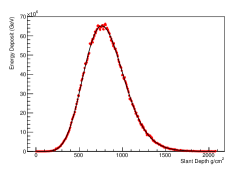
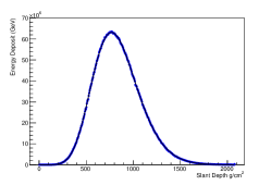
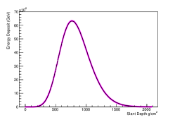
The thinning algorithm causes artificial fluctuations in the calculation of the shower development which needs to be taken into account. For example, figure 1 shows the longitudinal development of one shower simulated with three thinning factors , and . The first interaction altitude was fixed at 60 km and the target is Nitrogen nuclei. Sibyll2.1 was used for this study. It illustrates how the fluctuations of the simulated longitudinal profile increase with increasing thinning factor.
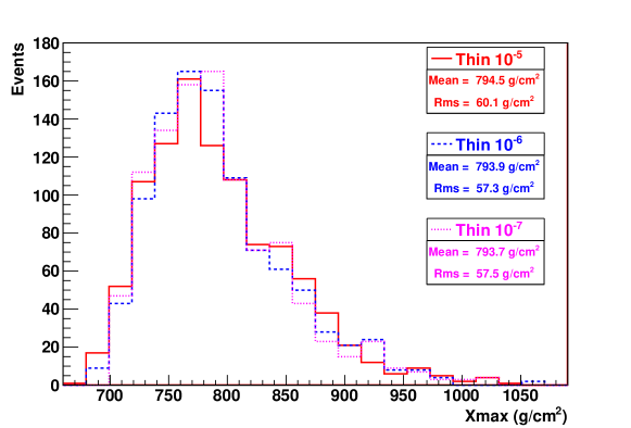
Figure 2 shows the distribution for 1000 simulated shower for three thinning factors. In this example the first interaction point and target were not fixed. Sibyll2.1 was used again for this study. Figure 2 shows that the and RMS are very similar for any thinning factor used. The maximum difference is 0.4 g/cm2 for and 2.8 g/cm2 for RMS. Based on this study we chose to simulate all showers with thinning factor .
2.3 Isobaric Nuclei Analysis
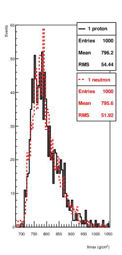
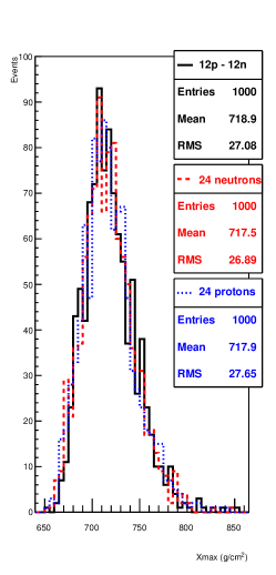
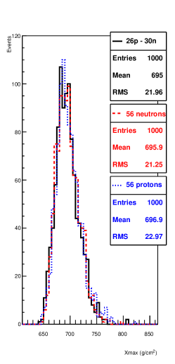
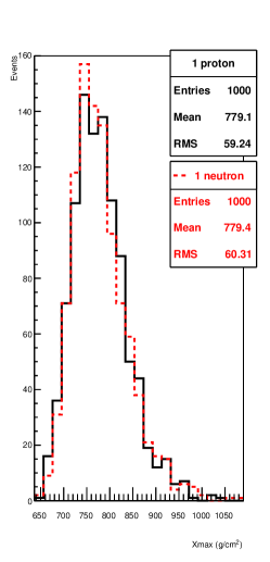
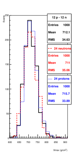
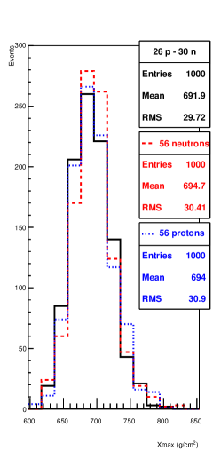
Some of the simulation used in this paper have been produced for another study and have been re-used in this work to save computational time. The previously simulated showers have exotic primary particle with unstable number of protons and neutrons. In this section we compare the longitudinal development of showers started with exotic nuclei with the shower started with stable nuclei with the same total number of nucleons. Our intention is to show that the development of a shower at high energies does not depend on the number of protons and neutrons independently but depends only on the total number of nucleons considered.
Corsika and Conex simulators differentiate isobaric nuclei by allowing the determination of the number of protons and neutrons of the primary nuclei. However the treatment of the first interaction is done by the hadronic interaction models. QGSJetII does not differentiate isobaric nuclei interactions, Sibyll2.1 does differentiate.
At the highest energies the energy loss of protons and neutrons is negligible when compared to the total energy and therefore only the total number of nucleons should influence the development of the shower. On the other hand, Coulomb dissociation should also be taken into account [coloumb:dissociation]. Nevertheless, none of the hadronic interaction models available include this effect and therefore the development of the simulated shower should not depend on the number of protons and neutrons in the nuclei.
Figure 3 shows the distribution for eV showers. We have simulated nuclei with different numbers of proton and neutron constituents. We can conclude that, at the energy range of interest, the predicted and the RMS does not depend on the number of protons and neutrons which form a nucleus with given mass A. The maximum difference in the was 2.9 g/cm2 for A = 24 and QGSJetII and in the RMS was 2.5 g/cm2 for A = 1 and Sibyll2.1.
3 Results
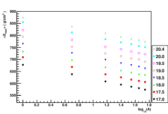
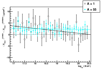
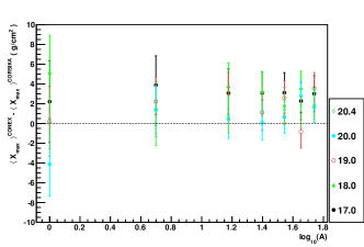
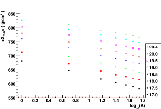
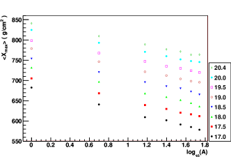
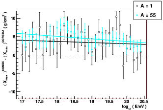
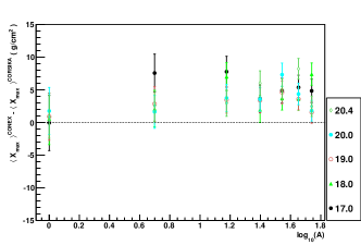
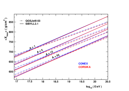
Figures 4 and 5 show the comparisons of using both simulators for Sibyll2.1 and QGSJetII respectively. Figures 4e and 4f show the difference between Corsika and Conex predictions as a function of energy and mass respectively when both programs used Sibyll2.1. The same is shown in figures 5e and 5f for QGSJetII. The differences between the predicted by Corsika and Conex are smaller than 7 g/cm2 in the parameter space studied by us. Conex tends to simulate showers slightly deeper than Corsika.
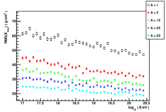
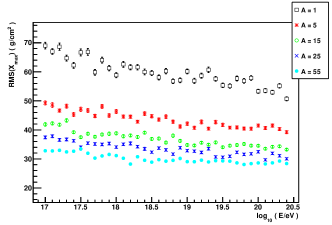
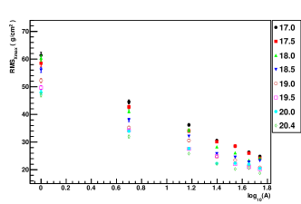
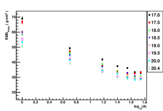
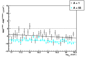
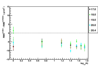
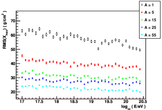
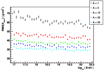
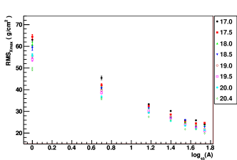
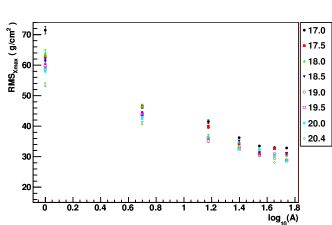
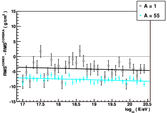
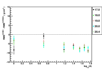
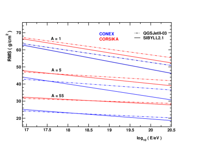
Similar results are presented in figures 6 and 7 for the RMS. In the parameter space studied by us the differences in the RMS calculated by Corsika and Conex are smaller than 8 g/cm2. No significant trend of the difference with energy or mass was seen.
The evolution of RMS shown in figure 6a, 6b, 7a and 7b shows large fluctuations apparently larger than the estimated statistical fluctuation. The statistical fluctuation shown as error bars of RMS is the standard statistical variance of the variance of a distribution. No Gaussian approximation was used. The trend of RMS with energy is statisticaly incompatible with a linear behavior. A linear fit of RMS versus energy shows a mean .
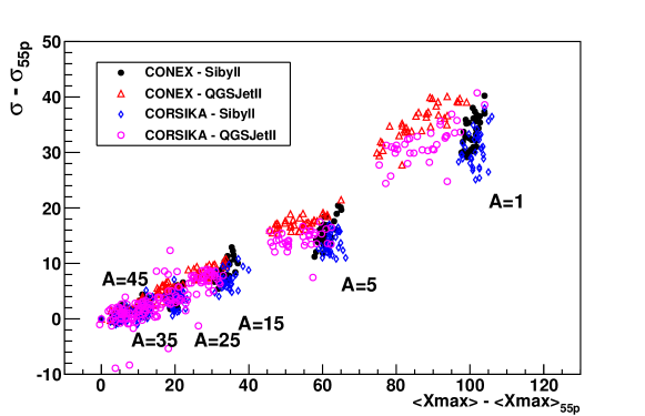
Figure 8 summarizes the differences in and RMS between the simulation programs and between the hadronic interaction models. This figure shows simultaneously the and RMS values, where the corresponding and RMS for a nuclei with mass 55 has been taken as reference (as suggested in [Kampert2012660]). This figure illustrates the importance of taking into account the simulation program differences into the systematic uncertainty of the model predictions. Each blob corresponds to the and RMS predictions for one primary particle at different energies.
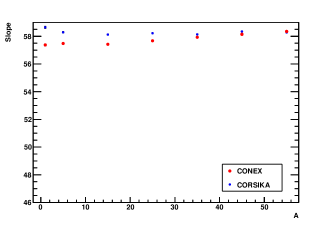
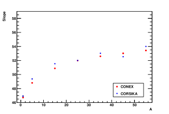
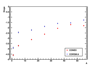
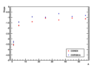
The elongation rate theorem [linsley__1977, t._k._gaisser__1979, linsley_validity_1981] proposes the use of the slope of the variation of with energy as a composition parameter. According to this proposal, changes in this slope represents changes in composition. Figure 9 show the slope of the variation of and RMS with energy as a function of primary particle mass for Corsika and Conex using Sibyll2.1 and QGSJetII. The slope in this figure corresponds to the fit of a straight line in the energy range ( eV). There is a good agreement between Conex and Corsika when the same hadronic model is used. The slope of the RMS when Sibyll2.1 is used presents the largest discrepancy between Conex and Corsika (see 9.c).
It has been shown before [bib:heck:presentation] that the dependencies of the and RMS are not strictly straight lines however the departure of the linear dependency is very small for energies above eV as studied here.
It is clear from figure 9 that the slope of the as a function of energy is dominated by the hadronic interaction model rather than by the shower simulation.
4 Parametrization of the distributions
The distributions can be described by a function which is a convolution of a Gaussian with an exponential [bib:gauss:expo]:
| (2) |
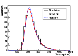
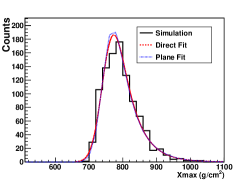
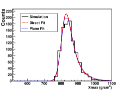
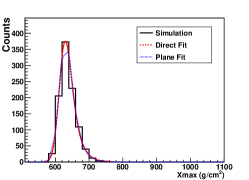
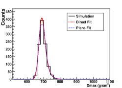
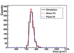
This equation has four parameters. is a normalization factor which gives the total number of events in the distribution. , and are parameters which are related to the decay factor of the exponential, the maximum of the distribution and the width of the distribution respectively. is the error function. We used this equation to fit the distributions of all mass and energies we have simulated. Figure 14 shows examples distributions we fit with this equation. The aim of this study is to use equation 2 to fit the distribution and calculate the and RMS. We show below that a convolution of a Gaussian with an exponential allows a good description of the and RMS. The proposed function is also a fairly good description of the distribution, see figures 14.
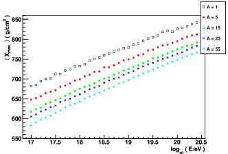
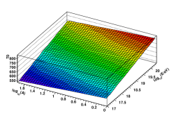
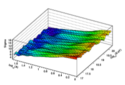
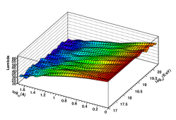
After that, we parametrized , and as a function of primary mass and energy using the simulated showers. Figure 10 show the evolution of the three parameters with energy and mass.
Figure 10a shows how has a very smooth dependence with mass and energy, recovering the already explored dependence of with mass and energy. On the other hand, and are not completely independent parameters. Both parameters influence the width of the distribution in different ways. The parameter changes the width of the distribution by modifying the decays of the exponential, making the high tail longer or shorter. also changes the width of the distribution by modifying the width of the central part. In fact, note that mathematically .
Given the degeneracy in shaping the width of the distribution, the parameters and are inversely correlated. The parameters and compensate each other, fluctuations to higher values of are correlated to fluctuations to smaller values of .
We performed a fit to plots in figure 10 with a linear dependence on and following equation:
| (3) |
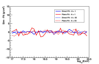
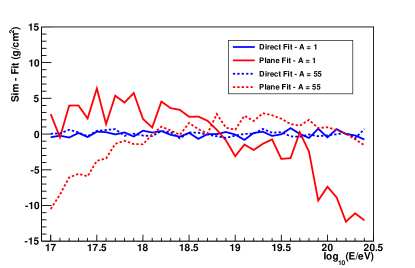
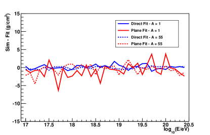
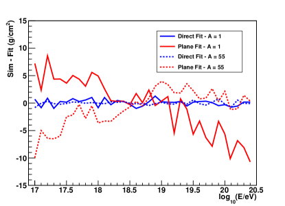
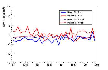
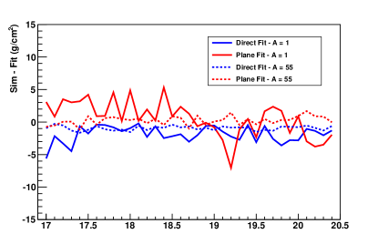
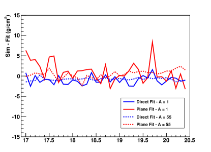
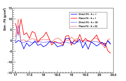
Tables 1 and 2 show the fitted parameters for Conex and Corsika respectively. Despite the fluctuations of and a linear fit in and is reasonably good approximation to describe the distribution. This can be seen in figures 11 and 12 where we show a comparison between the simulation, the direct fit of the distribution using equation 2 and the calculation using equation 3 and table 1.
It is clear that a direct fit of the distributions with equation 2 (blue lines) leads to a very good description of the first and second moments of the distribution. For all simulations and hadronic models in the entire energy range and for all primary particle used in our study the direct fit resulted in a difference on the simulation smaller than 2 g/cm2 for and smaller than 4 g/cm2 in the RMS.
The fit to a plane and is a reasonably good approximation to describe the distributions. This can be seen in figures 11 and 12 where we show a comparison between the simulation, the direct fit of the distribution using equation 2 and the calculation using equation 3 and table 1.
The parametrization as a function of energy and mass of the parameters that describe the Xmax distributions (equation 3) introduced some systematic errors in for the case of QGSJetII model (up to 10 g/cm2). This is shown with red lines in figure 11 (right hand side plots). The reason for this systematic errors is because the parametrization used (equation 3) is not the optimum one for QGSJetII model.
| Had. Model | ( err) | ( err) | ( err) | |
|---|---|---|---|---|
| QGSJetII | 53.06 (0.05) | -28.74 (0.12) | -275.93 (1.18) | |
| Sibyll2.1 | 60.48 (0.07) | -38.48 (0.13) | -402.80 (1.22) | |
| QGSJetII | -0.26 (0.06) | -5.63 (0.21) | 31.68 (3.38) | |
| Sibyll2.1 | -1.09 (0.07) | -5.28 (0.19) | 44.41 (1.54) | |
| QGSJetII | -2.68 (0.14) | -19.50 (0.43) | 100.32 (2.63) | |
| Sibyll2.1 | -2.61 (0.11) | -17.89 (0.14) | 96.28 (1.76) |
| Had. Model | ( err) | ( err) | ( err) | |
|---|---|---|---|---|
| QGSJetII | 53.32 (0.30) | -29.47 (0.52) | -283.93 (5.62) | |
| Sibyll2.1 | 60.77 (0.23) | -38.88 (0.31) | -408.88 (4.67) | |
| QGSJetII | 0.06 (0.002) | -5.06 (0.17) | 35.99 (3.21) | |
| Sibyll2.1 | -0.56 (0.08) | -4.70 (0.21) | 44.01 (2.03) | |
| QGSJetII | -1.73 (0.15) | -20.63 (0.34) | 82.69 (3.54) | |
| Sibyll2.1 | -2.49 (0.22) | -19.54 (0.34) | 96.04 (3.46) |
5 Conclusion
We have studied the simulation programs Corsika and Conex with the hadronic interaction models Sibyll2.1 and QGSJetII. We have shown that the and the RMS depend slightly on the combination of program and hadronic interaction model chosen. It is widely known that and RMS predicted by Sibyll2.1 and QGSJetII are different mainly due to the different extrapolations of the hadronic interaction properties to the highest energies. We have quantified here the differences between Corsika and Conex by predicting the and the RMS using the same hadronic interaction model. These differences are small, but should be considered as systematic uncertainties of the model predictions.
Figure 13 shows the evolution of the and RMS with energy. No clear dependency of the difference between Corsika and Conex with energy or primary particle type was seen. When using QGSJetII or Sibyll2.1, Corsika and Conex predict the with a difference smaller than 7 g/cm2, and the RMS with a difference smaller than 5 g/cm2. The differences in the slopes of a linear fit to the evolution of the and RMS with energy for Corsika and Conex are quite small ( %).
No assumption is made here for the cause of these differences. An investigation for the possible cause could be done, but in the meanwhile these differences between the programs should be considered as systematics error in the analysis of the and RMS when one tries to infer the composition abundance. Table 3 shows the suggested systematic uncertainties for the model predictions. Maximum values for the systematic uncertainties can be extracted from figures 4e, 5e, 6e and 7e.
| Hadronic Model | Mass (A) | systematic uncertainty suggested for the model predictions | ||
|---|---|---|---|---|
| RMS | Elongation rate | |||
| g/cm2 | g/cm2 | g/cm2 per energy decade | ||
| Sibyll2.1 | 1 | |||
| 55 | ||||
| QGSJetII | 1 | |||
| 55 | ||||
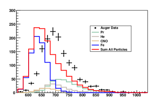
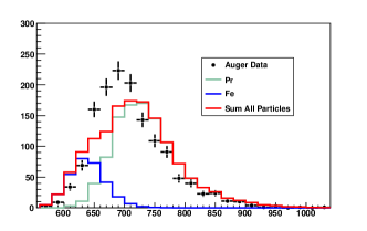
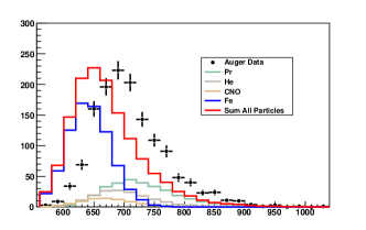
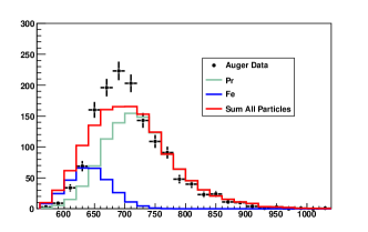
Section 4 shows the parametrization of the distributions as a function of energy and mass. The curves shown there can be used to estimate the first and second moments of the distribution from abundance calculations based on astrophysical arguments. As an example of the usage of this parametrization we have taken the astrophysical models developed by Berezinsky et al. [Berezinsky2004617] (Model 3) and Allard et al. [bib:allard] (Model A) and used our paremetrization to transform the abundance curves predicted by the models into a distribution. Figure 15 shows a distributions predicted by the models in comparison to the data measured by the Pierre Auger Observatory [bib:auger:xmax:icrc:2011]. We have convolved the model predictions with a Gaussian detector resolution of 20 g/cm2. The utility of the parametrization is such that the models can be compared to the distribution instead of only the and RMS.
6 Acknowledgments
We thank the financial support given by FAPESP(2008/04259-0, 2010/07359-6) and CNPq. We thank S.Ostapchenko, D. Heck, M. Unger, A. Bueno Villar, R. Engel, P. Gouffon, R. Clay and T. Pierog for reading this manuscript and sending us relevant suggestions.