Reservoir-engineered entanglement in optomechanical systems

Abstract

We show how strong steady-state entanglement can be achieved in a three-mode optomechanical system (or other parametrically-coupled bosonic system) by effectively laser-cooling a delocalized Bogoliubov mode. This approach allows one to surpass the bound on the maximum stationary intracavity entanglement possible with a coherent two-mode squeezing interaction. In particular, we find that optimizing the relative ratio of optomechanical couplings, rather than simply increasing their magnitudes, is essential for achieving strong entanglement. Unlike typical dissipative entanglement schemes, our results cannot be described by treating the effects of the entangling reservoir via a Linblad master equation.

Introduction– The study of highly entangled quantum states is of interest both for fundamental reasons and for a myriad of applications to quantum information processing and quantum communication. Of particular fundamental interest is the possibility to entangle distinct macroscopic objects, a task made difficult by the unavoidable decoherence and dissipation associated with such systems. Equally interesting would be the ability to entangle photons of very different frequencies, e.g. microwave and optical photons.

A promising venue for the realization of both these kinds of entanglement is provided by quantum optomechanics, where macroscopic mechanical degrees of freedom can be controlled, measured and coupled using the modes of an electromagnetic cavity. Recent milestones in this field include the ability to cavity-cool a mechanical resonator to its ground state of motion Teufel et al. (2011a); Chan et al. (2011) and the observation of many-photon strong coupling effects Weis et al. (2010); Safavi-Naeini et al. (2011); Teufel et al. (2011b); Verhagen et al. (2012). A natural setting for entanglement generation is a three-mode optomechanical system consisting of two “target” modes to be entangled, which are each coupled to a third “auxiliary” mode. One could either have two optical target modes and a mechanical auxiliary mode, or vice-versa; both variants have recently been achieved in experiment Hill et al. (2012); Dong et al. (2012); Massel et al. (2012). Several theoretical studies have described such schemes, using the basic idea that the auxiliary mode mediates an effective (coherent) two-mode squeezing interaction between the two target modes, see e.g. Mancini et al. (2002); Paternostro et al. (2007); Barzanjeh et al. (2011, 2012). However, such schemes typically yield at best a relatively small amount of intra-mode entanglement (something which we quantify more fully below).

In this paper, we again consider generating steady-state entanglement of two bosonic modes in a three-mode system; while we focus on an optomechanical realization, our ideas could also be realized using superconducting circuits coupled via Josephson junctions Bergeal et al. (2010); Peropadre et al. (2012) or other parametrically-coupled 3-bosonic-mode system. Unlike previous works, we consider the possibility of entanglement via reservoir engineering Poyatos et al. (1996): we wish to tailor the dissipative environment of the two target modes such that the dissipative dynamics relaxes the system into an entangled state. Such dissipative entanglement has been discussed in the context of atomic systems Plenio and Huelga (2002); Kraus and Cirac (2004); Parkins et al. (2006); Kraus et al. (2008); Krauter et al. (2011) and has even been realized experimentally Muschik et al. (2011).

The dissipative entanglement scheme we describe is related to optomechanical cavity-cooling schemes Marquardt et al. (2007); Wilson-Rae et al. (2007) which have been used successfully to cool mechanical resonators to the ground state. In our case, one is not cooling a simple mechanical mode to the ground state, but rather a hybrid mode delocalized over both target modes. In contrast to previous reservoir-engineering approaches to entanglement generation, where the dynamics is reduced to a simple Markovian master equation for the target degrees-of-freedom, our treatment is valid even in the regime where a simple adiabatic elimination of the intermediate mode is not possible. As we show, this regime turns out to be the most effective at generating entanglement. Our result shows that by optimizing the ratio of optomechanical coupling strengths, rather than simply increasing their magnitudes, this laser-cooling mechanism can be used to yield large amounts of time-independent intra-cavity entanglement. The amount of entanglement is far greater than in previous studies and, in fact, far greater than the maximum possible entanglement allowed by a coherent parametric interaction. Note that reservoir-engineering in optomechanics has previously been studied theoretically, with the very different goal of generating long-range coherence in arrays Tomadin et al. (2011).

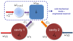
Figure 1: Schematic of one realization of a 3-mode optomechanical system, where two cavity modes are coupled to a single mode of a mechanical resonator. By driving cavity $1$ ($2$) at the red (blue) detuned mechanical sideband, a dissipative entanglement mechanism is realized. To enhance the scheme, the mechanical resonator is cavity cooled and optically damped via a coupling to a third driven cavity mode, so that its total damping rate $\gamma$ is greater than the cavity damping rates $\kappa$.

System and normal modes– While our scheme applies to a general bosonic three mode system, we focus here on an optomechanical system where two optical or microwave cavity modes are coupled to a single mode of a mechanical resonator (see Fig. 1); see the EPAPS EPA for a discussion of entangling two mechanical modes coupled to a cavity mode. The Hamiltonian is:

$$\hat{H}=\omega_{\rm M}\hat{b}^{\dagger}\hat{b}+\sum_{i=1,2}\left(\omega_{i}\hat{a}_{i}^{{\dagger}}\hat{a}_{i}+g_{i}\left(\hat{b}^{{\dagger}}+\hat{b}\right)\hat{a}_{i}^{\dagger}\hat{a}_{i}\right)+\hat{H}_{\rm diss}.$$ (1)

$\hat{a}_{i}$ is the annihilation operator for cavity $i$ (frequency $\omega_{i}$, damping rate $\kappa_{i}$), $\hat{b}$ is the annihilation operator of the mechanical mode (frequency $\omega_{\rm M}$, damping rate $\gamma$), and $g_{i}$ are the optomechanical coupling strengths. $\hat{H}_{\rm diss}$ describes the dissipation of each mode, as well as the driving of the cavity modes. To achieve an entangling interaction, cavity $1$ ($2$) is driven at the red (blue) sideband associated with the mechanical resonator: $\omega_{d1}=\omega_{1}-\omega_{\rm M}$ and $\omega_{d2}=\omega_{2}+\omega_{\rm M}$ Barzanjeh et al. (2011). We work in an interaction picture with respect to the cavity drives, and write $\hat{a}_{i}=\bar{a}_{i}+\hat{d}_{i}$ where $\bar{a}_{i}$ is the classical cavity amplitude. We take $|\bar{a}_{1,2}|\gg 1$, which allows us to linearize the optomechanical interaction in the usual way (i.e. drop interaction terms not enhanced by the classical cavity amplitudes). The linearized Hamiltonian in the rotating frame is thus $\hat{H}=\omega_{M}\left(\hat{b}^{\dagger}\hat{b}+\hat{d}_{1}^{\dagger}\hat{d}_{1}-\hat{d}_{2}^{\dagger}\hat{d}_{2}\right)+\hat{H}_{\rm int}+\hat{H}_{\rm CR}+\hat{H}_{\rm diss}$ with

$$\hat{H}_{\rm int} = G_{1}\left(\hat{b}^{{\dagger}}\hat{d}_{1}+\hat{d}_{1}^{{\dagger}}\hat{b}\right)+G_{2}\left(\hat{b}\hat{d}_{2}+\hat{d}_{2}^{{\dagger}}\hat{b}^{{\dagger}}\right),$$ (2)

$$\hat{H}_{\rm CR} = G_{1}\left(\hat{b}^{{\dagger}}\hat{d}^{\dagger}_{1}+\hat{d}_{1}\hat{b}\right)+G_{2}\left(\hat{b}^{\dagger}\hat{d}_{2}+\hat{d}_{2}^{{\dagger}}\hat{b}\right).$$ (3)

Here $G_{i}=g_{i}\bar{a}_{i}$ (we take $g_{i},\bar{a}_{i}>0$ without loss of generality). We further focus on the resolved-sideband regime $\omega_{\rm M}\gg\kappa_{1},\kappa_{2}$, which suppresses the effects of the non-resonant interactions in $\hat{H}_{CR}$. The remaining interaction $\hat{H}_{\rm int}$ in Eq. (21) has the basic form suitable for entangling $\hat{d}_{1}$ and $\hat{d}_{2}$: on a heuristic level, the parametric-amplifier interaction ($G_{2}$ term) first entangles $\hat{d}_{2}$ and $\hat{b}$, and then the beam-splitter interaction ($G_{1}$ term) swaps the $\hat{b}$ and $\hat{d}_{1}$ states, thus yielding the desired entanglement.

Note that if one made the interactions in Eq. (21) non-resonant (e.g. by detuning the cavity drives from the sideband resonances by $\Delta$), one could adiabatically eliminate the mechanical mode, resulting in a two-mode squeezing interaction $\hat{H}_{\rm TMS}\simeq\lambda\left(\hat{d}_{1}\hat{d}_{2}+{\rm h.c.}\right)$ with $\lambda\sim G_{1}G_{2}/\Delta$ Schmidt et al. (2012). Such an interaction naturally leads to entanglement, but the amount is severely limited by the requirement of stability $\lambda\leq\kappa_{1,2}/2$. We quantify the entanglement using the standard measure of the logarithmic negativity $E_{N}$ EPA . One finds that the maximum stationary intracavity entanglement due to the two-mode squeezing coupling is (for $\kappa_{1}=\kappa_{2}$ and zero temperature) $E_{N}=\ln(1+2\lambda/\kappa)\leq\ln 2\sim 0.7$. Many suggested schemes for entanglement generation in optomechanical systems are limited by this stability requirement.

In contrast, the resonant case we consider allows for an alternative dissipative entanglement mechanism capable of much larger $E_{N}$. We will focus attention on the regime $G_{2}<G_{1}$ where (for $\kappa_{1}=\kappa_{2}$) our linear system is always stable EPA . Defining the effective two-mode squeezing parameter $r=\mathrm{arctanh}(G_{2}/G_{1})$, we introduce delocalized (canonical) cavity Bogoliubov mode operators:

$$\hat{\beta}_{A} = \hat{d}_{1}\cosh r+\hat{d}_{2}^{{\dagger}}\sinh r\equiv\hat{S}\left(r\right)\hat{d}_{1}\hat{S}^{{\dagger}}\left(r\right),$$

$$\hat{\beta}_{B} = \hat{d}_{1}^{{\dagger}}\sinh r+\hat{d}_{2}\cosh r\equiv\hat{S}\left(r\right)\hat{d}_{2}\hat{S}^{{\dagger}}\left(r\right).$$ (4)

Here, $\hat{S}\left(r\right)\equiv\exp\left[r\hat{d}_{1}\hat{d}_{2}-h.c.\right]$ is a two-mode squeezing operator. It thus follows that the joint vacuum of $\hat{\beta}_{A},\hat{\beta}_{B}$ is the two-mode squeezed state $|r\rangle=\hat{S}(r)|0,0\rangle$, where $|0,0\rangle$ is the vacuum of $\hat{d}_{1},\hat{d}_{2}$. The entanglement of this state is simply $E_{N}=2r$.

In terms of these new operators, $\hat{H}_{0}=\omega_{\rm M}\left(\hat{b}^{\dagger}\hat{b}+\hat{\beta}_{A}^{\dagger}\hat{\beta}_{A}-\hat{\beta}_{B}^{\dagger}\hat{\beta}_{B}\right)$ and the optomechanical interactions in Eq. (21) and (3) take the simple form

$$\hat{H}_{\rm int}=\tilde{G}\hat{\beta}_{A}^{\dagger}\hat{b}+h.c.,\;\;\;\;\hat{H}_{\rm CR}=\tilde{G}\hat{\beta}_{A}^{\dagger}\hat{b}^{\dagger}+h.c.,$$ (5)

where $\tilde{G}\equiv\sqrt{G_{1}^{2}-G_{2}^{2}}$. The mode $\hat{\beta}_{B}$ completely decouples from the mechanics (it is a mechanically-dark mode Wang and Clerk (2012); Tian (2012)), while in the good-cavity limit of interest $\hat{H}_{\rm CR}$ can be neglected, implying that the mode $\hat{\beta}_{A}$ has a simple beam-splitter interaction with the mechanics. $\hat{H}_{0}+\hat{H}_{\rm int}$ is trivially diagonalized, resulting in hybridized modes $\hat{\beta}_{\pm}=\left(\hat{\beta}_{A}\pm\hat{b}\right)/\sqrt{2}$ with energies $\omega_{\rm M}\pm\tilde{G}$. The existence of three distinct eigenmodes (two hybrid, one dark) can be useful to understand entanglement (in particular spectral entanglement Barzanjeh et al. (2012); Wipf et al. (2008)) in the case where the mechanical mode is driven by excessive thermal noise; we will discuss this in a future work. We focus here on generating intracavity entanglement, which has the benefit of being insensitive to whether internal losses contribute to the damping rate $\kappa$ of the cavities.

We now exploit the fact that Eq. (5) has exactly the form used for standard cavity cooling Marquardt et al. (2007); Wilson-Rae et al. (2007). Thus, if we can couple the mechanical mode $\hat{b}$ to a cold reservoir, then the beam-splitter coupling $\hat{H}_{\rm int}$ can be used to cool $\hat{\beta}_{A}$ towards vacuum, resulting in a stationary entangled state. A high-frequency, low-$Q$ mechanical resonator would thus be ideal. Alternatively, we will take the mechanical mode to be coupled to a third cavity mode which is used to laser cool its thermal occupancy towards the ground state by providing a source of cold damping, see Fig. 1. In what follows, we include the cooling cavity coupled to the mechanical resonator in the definition of its effective thermal bath; hence, the damping rate $\gamma$ includes the large contribution of the optical damping. Amusingly, our scheme is one of the few examples in optomechanics where the enhanced mechanical damping rate resulting from cavity cooling is actually highly beneficial.

Langevin equations & cavity cooling– To describe the cooling potential of $\hat{H}_{\rm int}$, we next use input-output theory to derive the Heisenberg-Langevin equations for our linearized system. These take the standard form:

$$\frac{d}{dt}\hat{b} = \left(-i\omega_{\rm M}-\frac{\gamma}{2}\right)\hat{b}-i\left(G_{1}\hat{d}_{1}+G_{2}\hat{d}_{2}^{{\dagger}}\right)-\sqrt{\gamma}\hat{b}_{\mathrm{in}},$$

$$\frac{d}{dt}\hat{d}_{1} = \left(-i\omega_{\rm M}-\frac{\kappa_{1}}{2}\right)\hat{d}_{1}-iG_{1}\hat{b}-\sqrt{\kappa_{1}}\hat{d}_{1,\mathrm{in}},$$

$$\frac{d}{dt}\hat{d}_{2}^{{\dagger}} = \left(-i\omega_{\rm M}-\frac{\kappa_{2}}{2}\right)\hat{d}_{2}^{{\dagger}}+iG_{2}\hat{b}-\sqrt{\kappa_{2}}\hat{d}_{2,\mathrm{in}}^{{\dagger}},$$ (6)

where $\hat{d}_{i,\rm in},\hat{b}_{\rm in}$ describes operator-valued white noise driving the cavity and mechanical modes, and we have taken the good-cavity limit $\omega_{\rm M}\gg\kappa$ (allowing us to drop terms due to $\hat{H}_{\rm CR}$). Eqs. (6) are readily solved to find the steady-state occupancy and correlation of the Bogoliubov modes. In the following analytic expressions, we take $\kappa_{1}=\kappa_{2}$ for simplicity and focus on the good-cavity limit (though Fig. 2 includes corrections due to $\hat{H}_{\rm CR}$).

Imagine first that the optomechanical interactions vanished, i.e. $\hat{H}_{\rm int}=0$, and consider the behaviour of $\hat{\beta}_{A},\hat{\beta}_{B}$ (defined for a fixed $r>0$). Even at zero temperature, $\hat{\beta}_{A}$ and $\hat{\beta}_{B}$ will have a non-zero occupancy: the Bogoliubov transformation of Eq. (4) implies that vacuum noise driving the cavities acts as effective thermal noise for $\hat{\beta}_{A},\hat{\beta}_{B}$. Writing these intrinsic ($\hat{H}_{\rm int}=0$) occupancies as $\left\langle\hat{\beta}_{j}^{\dagger}\hat{\beta}_{j}\right\rangle_{0}=\bar{n}_{{\rm th},j}$ we have

$$\bar{n}_{{\rm th},A/B}=\bar{n}_{{\rm th},1/2}\cosh^{2}r+\left(\bar{n}_{{\rm th},2/1}+1\right)\sinh^{2}r.$$ (7)

Here, $\bar{n}_{\mathrm{th},1}$ ($\bar{n}_{\mathrm{th},2}$) represents the temperature of the thermal bath coupled to mechanical resonator $1$ ($2$). As one increases the squeeze parameter $r$, the effective heating of the $\hat{\beta}_{j}$ modes becomes exponentially large, implying the state of the system is far from being an ideal two-mode squeezed vacuum state; the state is not entangled.

Including now the effects of $H_{\rm int}$ (and taking $r=\mathrm{arctanh}(G_{2}/G_{1})$), the dark-mode $\hat{\beta}_{B}$ is unaffected, whereas the occupancy of $\hat{\beta}_{A}$ is modified to

$$\left\langle\hat{\beta}_{A}^{{\dagger}}\hat{\beta}_{A}\right\rangle = \frac{\kappa}{\Gamma_{\rm opt}+\kappa}\left(1+\frac{\Gamma_{\rm opt}}{\gamma+\kappa}\right)\bar{n}_{\mathrm{th},A}+$$ (8)

$$\frac{\Gamma_{\rm opt}\gamma}{(\Gamma_{\rm opt}+\kappa)(\gamma+\kappa)}\bar{n}_{\rm th,M}.$$

where $\bar{n}_{\rm th,M}$ represents the temperature of the mechanical bath (which includes the cooling cavity), and the effective “cold damping rate” of $\hat{\beta}_{A}$ by the mechanics is $\Gamma_{\rm opt}\equiv 4\tilde{G}^{2}/\gamma$. This is the familiar equation for cavity cooling in the good-cavity limit, where now the mechanics plays the role of a cold reservoir. For $\bar{n}_{\rm th,M}=0$ and weak coupling ($\Gamma_{\rm opt}\ll\gamma$), the $\hat{\beta}_{A}$ mode is cooled by a factor $\kappa/(\kappa+\Gamma_{\rm opt})$. In the strong coupling limit, the cooling factor saturates to a value $\kappa/(\gamma+\kappa)$.

Thus, while even vacuum noise tends to heat $\hat{\beta}_{A}$, $\hat{\beta}_{B}$ to an exponentially-large effective temperature, the optomechanical interaction of Eq. (5) can be used to cool $\hat{\beta}_{A}$. Using the inequality of Duan et al. Duan et al. (2000), one can show that if one cools $\hat{\beta}_{A}$ so that

$$\langle\hat{\beta}_{A}^{\dagger}\hat{\beta}_{A}\rangle\leq\sinh^{2}r,$$ (9)

then the two cavities must necessarily be entangled EPA . As the orthogonal Bogoluibov mode $\hat{\beta}_{B}$ is decoupled from the mechanics, it is not cooled, making it impossible to achieve an ideal two-mode squeezed vacuum state. Nonetheless, we find that simply cooling $\hat{\beta}_{A}$ is sufficient to generate a steady state with significant entanglement ($E_{N}\sim 2r-\ln 2$ in the large $r$ limit); this is despite the fact that the resulting state has negligible overlap with a two-mode squeezed vacuum (see EPAPS EPA ).

To rigorously quantify the cavity-cavity entanglement, we compute and discuss in what follows the log negativity $E_{N}$, which is a function of the covariance matrix; details are provided in the supplementary material EPA .

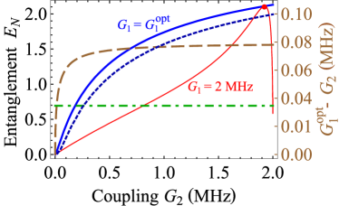
Figure 2: Stationary intra-cavity entanglement (as quantified by log negativity $E_{N}$, left scale) as a function of the entangling interaction $G_{2}$. We take $\bar{n}_{{\rm th},1}=\bar{n}_{{\rm th},2}=0$, a mechanical frequency of $\omega_{\rm M}=2\pi\times 10\text{ MHz}$ and damping $\gamma=2\pi\times 0.8\text{ MHz}$, and do not make the rotating wave approximation. The solid red thin curve corresponds to a fixed value of $G_{1}=2\pi\times 2\text{ MHz}$, and $\kappa_{1}=\kappa_{2}=2\pi\times 50\text{ kHz}$. One clearly sees a non-monotonic dependence on $G_{2}$. The solid blue thick curves and short-dashed blue curves instead correspond to tuning $G_{1}$ to the value $G_{1}^{\mathrm{opt}}$ for each $G_{2}$, such that the dissipative entangling mechanism can be optimized. The value of $G_{1}^{\mathrm{opt}}-G_{2}$ (c.f. Eq. (10)) is indicated by the long-dashed brown curve (right scale). The solid blue (dashed blue) corresponds to $\kappa_{1}=\kappa_{2}=50\text{ kHz}$ ($\kappa_{1/2}/2\pi=45\text{ kHz}$, $55\text{ kHz}$) and $\bar{n}_{\rm th,M}=0$ ($\bar{n}_{\rm th,M}=0.3$). The green dash-dot line represents the maximum stationary entanglement achievable with a coherent two-mode squeezing interaction, $E_{N}=\ln 2$.

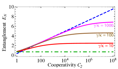
Figure 3: Intra-cavity stationary entanglement (quantified by $E_{N}$) versus cooperativity $C_{2}$, where we use an optimized choice for $G_{1}$ (as given by Eq. (10)), and have taken $\kappa_{1}=\kappa_{2}$ and zero temperature. The solid lines correspond to different choices of the damping ratio $\gamma/\kappa$ as indicated; increasing $\gamma/\kappa$ increases the amount that one can cool the delocalized $\hat{\beta}_{A}$ mode, and hence enhances entanglement. For large $C_{2}$, these curves asymptote to the value in Eq. (12). The dashed blue line is the asymptotic expression of Eq. (11). The green dashed-dotted line indicates $E_{N}=\ln 2$ (the maximum $E_{N}$ possible with a two-mode squeezing interaction).

Maximizing entanglement– We now see that entanglement generation is more subtle than one might expect given the simple form of Eq. (21). In particular, if $G_{1}$ is fixed, the amount of stationary entanglement is a non-monotonic function of the entangling-interaction strength $G_{2}$ (see Fig. 2). The dissipative entanglement mechanism discussed here directly explains this behaviour, as increasing $G_{2}$ has two opposing effects: it not only increases $r$ and the delocalization of the Bogoliubov modes (enhancing entanglement), but also increases the effective temperature of these modes. This latter effect is due both to an increase in the effective temperature of the cavity vacuum noise (c.f. Eq. (7)), and to a suppression of the cavity-cooling effect (as the effective coupling $\tilde{G}$ decreases with increasing $G_{2}$).

The maximum entanglement is achieved by carefully balancing the opposing tendencies described above; without this optimization, the entanglement will remain small. For fixed couplings $G_{1},G_{2}$, one can optimize the entanglement as a function of the mechanical damping $\gamma$. The maximum occurs at a non-zero dissipation strength, which at zero mechanical temperature and in the good-cavity limit is simply given by $\gamma=2\tilde{G}$. This value simply minimizes the occupancy of $\hat{\beta}_{A}$, and corresponds to a simple impedance matching condition (i.e. the rate with which the $\hat{\beta}_{A}$ mode and mechanics exchange energy matches the rate at which the mechanics and its bath exchange energy).

More relevant to experiment is to consider $\kappa$ and $\gamma$ fixed, and optimize the entanglement over coupling strength. Focusing on the most interesting regime where the cooperativity $C_{2}\equiv G_{2}^{2}/(\gamma\kappa)\gg 1$, and considering the good-cavity limit and zero temperature (the mechanical resonator is also cooled to vacuum by the 3rd cavity mode), we find that for fixed $G_{2}$, the optimal $G_{1}$ is given by

$$G_{1}^{\rm opt}\approx G_{2}+\sqrt{\frac{\kappa\gamma}{8}}\left(1+\frac{2\kappa}{\gamma}\right),\;\;\;\textrm{i.e. }\frac{\tilde{G}^{\rm opt}}{\gamma}\approx\left(\frac{C_{2}\kappa^{2}}{2\gamma^{2}}\right)^{1/4}.$$ (10)

Note that for large $C_{2}$, this optimal value can easily correspond to a strong interaction $\tilde{G}>\kappa,\gamma$. Thus, in this optimal regime, the effects of our “engineered reservoir” (cold mechanical resonator) on the target cavity modes cannot be described by a Markovian dissipator in a master equation; this is in stark contrast to standard dissipation-by-entanglement schemes.

For the optimal value of $G_{1}$ above, the entanglement takes simple forms in two relevant limits. If we hold $C_{2}$ fixed while taking the limit $\gamma/\kappa\rightarrow\infty$, we have (at zero temperature):

$$E_{N}^{\mathrm{opt}}\approx\frac{1}{2}\ln\left[2C_{2}\right]=2r-2\ln 2$$ (11)

For large $C_{2}$, the entanglement is almost that of a two-mode squeezed vacuum (i.e. $E_{N}=2r$). Alternatively, we could hold the ratio $\gamma/\kappa$ fixed and let $C_{2}\rightarrow\infty$, we have (at zero temperature):

$$E_{N}^{\mathrm{opt}}\sim\ln\left(2+\frac{\gamma}{\kappa}+\mathcal{O}\left[\frac{(\gamma/\kappa)^{2}}{\sqrt{C_{2}}}\right]\right)$$ (12)

This is the strong-interaction limit, where the $\hat{\beta}_{A}$ mode hybridizes with the mechanical resonator. The maximal cooling of $\hat{\beta}_{A}$ is consequently set by the ratio $\gamma/\kappa$ (c.f. Eq. (8)). The amount of entanglement here increases monotonically from $\ln 2$ (the maximum possible with a coherent coupling) as this cooling factor is increased.

The behaviour of the stationary entanglement versus coupling strength is shown in Fig. 2, where we have used parameters similar to those achieved in recent state-of-the-art experiments on microwave-circuit optomechanical systems Teufel et al. (2011b, a). We assume that a $\omega_{\rm M}=10\text{ MHz}$ mechanical resonator is first cavity cooled to near its ground state, with a final damping rate of $\gamma=0.8\text{ MHz}$ (which is predominantly due to the cold optical damping used for the cooling). By then optimally tuning the couplings to the target modes $G_{1},G_{2}$ to optimize the dissipative entanglement mechanism (while keeping them $\lesssim 2.2\text{ MHz}$), one can obtain a relatively large $E_{N}\sim 2.1$. This exceeds by an order-of-magnitude the intra-cavity entanglement obtained in previous studies of the same system Barzanjeh et al. (2011), as well as the the maximum of $\ln 2$ possible with a coherent two-mode squeezing interaction. If this entanglement was used for a teleportation experiment, the maximum possible fidelity would be $0.89$ Adesso and Illuminati (2005); Mari and Vitali (2008); this reduces the error by a factor of three compared to what would be possible with $E_{N}=\ln 2$. Fig. 2 also shows that large values of $E_{N}$ are possible even when $\bar{n}_{\rm th,M}\neq 0$ and $\kappa_{1}\neq\kappa_{2}$.

In Fig. 3 we show how the stationary entanglement grows to dramatically large values with $C_{2}$ for an optimized choice of $G_{1}$. While the parameters needed for such $E_{N}$ may be out of reach in current-generation optomechanics experiments, they may be more feasible by implementing a superconducting circuit realization of our scheme Bergeal et al. (2010); Peropadre et al. (2012).

Conclusions– We have presented a general method for the dissipative generation of entanglement in a three-mode optomechanical system. The entanglement generated here could be verified by measuring the covariance matrix of the two target cavity modes using homodyne techniques (see e.g. Paternostro et al. (2007)). Alternatively, one could directly use the cavity output spectra at resonance to measure the occupancy of the $\hat{\beta}_{A}$ mode; verifying that it violates the Duan inequality of Eq. (9) would also confirm the generation of entanglement (see EPA ).

We thank S. Chesi and L. Tian for useful conversations. This work was supported by the DARPA ORCHID program under a grant from the AFOSR.

I Supplemental information

I.1 System stability condition

The linearized Heisenberg-Langevin equations for our three mode system are given in Eqs. (6) of the main text. If we drop the noise terms, these equations take the form $\vec{v}=\mathbf{M}\cdot\vec{v}$ where $\vec{v}=(\hat{b},\hat{d}_{1},\hat{d}_{2}^{\dagger})$ and $\mathbf{M}$ is a $3\times 3$ matrix. For the system to be stable, we require that the eigenvalues of $\mathbf{M}$ all have a negative real part. This requirement leads to the well-known Routh-Hurwitz stability conditions. In the simple case $\kappa_{1}=\kappa_{2}$, the stability conditions reduce to the following necessary and sufficient condition:

$$\tilde{G}^{2}>-\frac{\kappa\gamma}{4}$$ (13)

Thus, if $\kappa_{1}=\kappa_{2}$ and $G_{2}\leq G_{1}$, the system is always stable (regardless of the magnitude of the cavity and mechanical damping rates).

In contrast, if $\kappa_{1}\neq\kappa_{2}$, then the stability conditions are modified such that the system can be unstable at $\tilde{G}=0$. While the general form of the conditions is somewhat unwieldy, in the interesting large cooperativity limit (i.e.  $C_{i}\equiv G_{i}^{2}/(\kappa_{i}\gamma)\gg 0$), they reduce to:

$$\tilde{G}^{2}>\bar{C}\gamma\max\left[\kappa_{1}-\kappa_{2},\frac{\kappa_{2}^{2}-\kappa_{1}^{2}}{2\gamma+\kappa_{1}+\kappa_{2}}\right]$$ (14)

with $\bar{C}\equiv(G_{1}^{2}+G_{2}^{2})/(\gamma(\kappa_{1}+\kappa_{2}))$. Note that in the $\gamma\gg\kappa_{1},\kappa_{2}$ limit of interest, this condition is very sensitive to the sign of $\kappa_{1}-\kappa_{2}$. On a heuristic level, damping asymmetry leads to negative damping terms in the equations of motion for the modes $\hat{\beta}_{A},\hat{\beta}_{B}$. For $\kappa_{1}<\kappa_{2}$ (and $\tilde{G}>0$), it is $\hat{\beta}_{A}$ which experiences negative damping; this is overwhelmed by the positive cold damping $\Gamma_{\mathrm{opt}}$ provided by the interaction with the mechanics (c.f. Eq. (8) in the main text), and hence there is no possibility of instability. In contrast, if $\kappa_{1}>\kappa_{2}$, it is the dark mode $\hat{\beta}_{B}$ which experiences negative damping; as there is nothing to offset this, the system can become unstable.

I.2 Definition of the logarithmic negativity

In this paper, unless specified, we use the logarithmic negativity $E_{N}$ to quantify the degree of entanglement; this quantity is a rigorous entanglement monotone, and is zero for separable states. For two-mode Gaussian states of sort realized by the two cavity modes $\hat{d}_{1},\hat{d}_{2}$ in our system, it can be calculated using the expression Vidal et al. (2009)

$$E_{N}=\max[0,-\ln 2\eta^{-}]$$ (15)

with

$$\eta^{-}=\frac{1}{\sqrt{2}}\sqrt{\Sigma-\sqrt{\Sigma^{2}-4\det\mathbf{V}}}$$ (16)

and

$$\Sigma=\det\mathbf{B}+\det\mathbf{B}^{\prime}-2\det\mathbf{C}.$$ (17)

Here $\mathbf{V}$ is the $4\times 4$ covariance matrix of the two modes of interest, defined via $V_{jj^{\prime}}=\frac{1}{2}\left\langle\Delta\hat{\xi}_{j}\Delta\hat{\xi}_{j^{\prime}}+\Delta\hat{\xi}_{j^{\prime}}\Delta\hat{\xi}_{j}\right\rangle$, with $\Delta\hat{\xi}_{j}=\hat{\xi}_{j}-\langle\hat{\xi}_{j}\rangle$ and $\hat{\vec{\xi}}=\left\{\hat{x}_{1},\hat{p}_{1},\hat{x}_{2},\hat{p}_{2}\right\}$. Here $\hat{x}_{i}=\left(\hat{d}_{i}+\hat{d}_{i}^{{\dagger}}\right)/\sqrt{2}$ and $\hat{p}_{i}=-i\left(\hat{d}_{i}-\hat{d}_{i}^{{\dagger}}\right)/\sqrt{2}$ and $\left[\hat{d}_{i},\hat{d}_{j}^{{\dagger}}\right]=\delta_{ij}$. The matrix $\mathbf{B}$, $\mathbf{B}^{\prime}$ and $\mathbf{C}$ are $2\times 2$ matrices related to the covariance matrix $\mathbf{V}$ as

$$\mathbf{V=}\left(\begin{array}[]{cc}\mathbf{B}&\mathbf{C}\\ \mathbf{C}^{T}&\mathbf{B}^{\prime}\end{array}\right).$$ (18)

The evaluation of entanglement needs the full information of the covariance matrix. In our main text, the relevant system consists of two cavity modes $\hat{d}_{1}$ and $\hat{d}_{2}$, or equivalently $\hat{\beta}_{A}$ and $\hat{\beta}_{B}$. Thus we also the correlation of $\hat{\beta}_{A}$ and $\hat{\beta}_{B}$, beside their occupancy (Eqs. (7) and (8) in the main text). The only non-zero correlator (again working in the good-cavity limit $\omega_{\mathrm{M}}\gg\kappa_{1},\kappa_{2}$ where the counter-rotating terms $\hat{H}_{CR}$ have negligible effect) is

$$\left\langle\hat{\beta}_{A}\hat{\beta}_{B}\right\rangle=\frac{\kappa\left(\kappa+\gamma\right)}{\Gamma_{\mathrm{opt}}\gamma+2\kappa\left(\kappa+\gamma\right)}(\bar{n}_{\mathrm{th},1}+\bar{n}_{\mathrm{th},2}+1)\sinh 2r.$$ (19)

I.3 Entanglement of mechanical resonators mediated by a cavity mode

While the main text focuses on a 3-mode optomechanical system having two cavity modes coupled to a single mechanical mode, our entanglement-by-dissipation scheme is very general, and can be applied in principle to any set of three parametrically-coupled bosonic modes. In particular, it could be realized in a 3-mode optomechanical system where two mechanical modes are coupled to a single cavity mode. We analyze this case below. Note that after this work was submitted, a paper by Tan et al. appeared which also analyzes dissipative entanglement of two mechanical resonators coupled to a cavity Tan et al. (2013); unlike our analysis before, this work does not explicitly consider the effect of non-RWA terms, terms we find to be especially problematic.

The starting Hamiltonian is now

$$\hat{H}=\omega_{\mathrm{cav}}\hat{a}^{\dagger}\hat{a}+\sum_{i=1,2}\left(\omega_{i}\hat{b}_{i}^{{\dagger}}\hat{b}_{i}+g_{i}\left(\hat{b}_{i}^{{\dagger}}+\hat{b}_{i}\right)\hat{a}^{\dagger}\hat{a}\right)+\hat{H}_{\mathrm{diss}}.$$ (20)

Here $\hat{b}_{i}$ is the annihilation operator of the $i$-th mechanical resonator (frequency $\omega_{i}$, damping rate $\gamma_{i}$), $\hat{a}$ is the annihilation operator of the auxiliary cavity mode (frequency $\omega_{\mathrm{cav}}$, damping rate $\kappa$), and $g_{i}$ are the optomechanical coupling strengths. $\hat{H}_{\mathrm{diss}}$ describes the dissipation of each mode, as well as the driving of the cavity mode.

To achieve an entangling interaction, we will drive the cavity mode at two frequencies $\omega_{d1}=\omega_{\mathrm{cav}}-\omega_{1}$ and $\omega_{d2}=\omega_{\mathrm{cav}}+\omega_{2}$ (i.e. the red(blue) sideband associated with mechanical resonator $1$ ($2$)). We can then write the cavity annihilation operator as $\hat{a}=\bar{a}(t)+\hat{d}e^{-i\omega_{\mathrm{cav}}t}$, where the classical cavity amplitude $\bar{a}(t)=\left(\bar{a}_{1}e^{i\omega_{1}t}+\bar{a}_{2}e^{-i\omega_{2}t}\right)e^{-i\omega_{\mathrm{cav}}t}$ is obtained from the classical equations of motion, with the sideband amplitudes $\bar{a}_{1,2}$ determined independently by the two cavity drives. We take $|\bar{a}_{1,2}|\gg 1$ which allows us to linearize the optomechanical interaction in the usual way (i.e. we drop interaction terms not enhanced by the classical cavity amplitude). Working in an interaction picture with respect to $\hat{H}_{0}=\omega_{1}\hat{b}_{1}^{{\dagger}}\hat{b}_{1}+\omega_{2}\hat{b}_{2}^{{\dagger}}\hat{b}_{2}+\omega_{\mathrm{cav}}\hat{d}^{{\dagger}}\hat{d}$, the linearized Hamiltonian in the displaced frame can be written as $\hat{H}=\hat{H}_{\mathrm{int}}+\hat{H}_{\mathrm{CR}}+\hat{H}_{\mathrm{diss}}$ with

$$\hat{H}_{\mathrm{int}}=G_{1}\left(\hat{d}^{{\dagger}}\hat{b}_{1}+\hat{d}\hat{b}_{1}^{{\dagger}}\right)+G_{2}\left(\hat{d}\hat{b}_{2}+\hat{d}^{{\dagger}}\hat{b}_{2}^{{\dagger}}\right).$$ (21)

Here $G_{i}=g_{i}\bar{a}_{i}$ (we take $g_{i}$, $\bar{a}_{i}$ to be positive without loss of generality) and $\hat{H}_{\mathrm{CR}}$ describes counter-rotating terms with an explicit time-dependence. Eq. (21) takes the same form as Eq. (2) in the main text and can be used for entangling $\hat{b}_{1}$ and $\hat{b}_{2}$ by reservoir engineering.

As discussed in the main text, the dissipative entanglement mechanism is optimal when the mode acting as the engineered reservoir is both cold and has a large damping rate compared to the target modes, as this allows optimal cooling of the Bogoliubov mode $\hat{\beta}_{A}$. This occurs naturally here, as the reservoir mode is a cavity mode, which given its higher frequency (compared to mechanical modes) will be naturally closer to the ground state, and which naturally has a large damping rate (i.e. its damping $\kappa$ will be much larger than the damping rates $\gamma$ of the target mechanical modes, by a factor $\sim 10^{4}$ to $10^{5}$ in typical optomechanical experiments). An additional benefit here is that since the mechanical damping rate $\gamma$ is small, the cooperativity of the system can reach a much larger value (in the strong coupling limit, $C$ can reach $10^{6}$). Thus the entanglement can easily reach $E_{N}\sim 7$ (as shown in Fig. 3), corresponding to teleportation fidelity of $99.9\%$. In contrast, the two-cavities-plus-mechanics scheme in the main text requires one to optically damp the mechanical damping $\gamma$ to a large value.

While the above features are extremely attractive, the downside of this scheme comes when one considers the non-resonant, counter-rotating terms. For the setup discussed in the main text (two cavities, one mechanical resonator), the counter-rotating terms only lead to a very small heating of the coupled $\hat{\beta}_{A}$ mode, much like standard optomechanical cavity cooling (c.f. Eq. (5) in the main text). In contrast, the situation here (two mechanical resonators, one cavity) is more complex. In general there are two sets of non-resonant, counter-rotating terms. The first are “diagonal terms”, where, e.g., the cavity drive at $\omega_{\mathrm{cav}}-\omega_{1}$ induces Stokes scattering with mechanical resonator 1. In our rotating frame, these take the form:

$$H_{\mathrm{CR}}^{A}=\left(\bar{a}_{1}^{\ast}g_{1}\hat{d}\hat{b}_{1}e^{-2i\omega_{1}t}+h.c.\right)+\left(\bar{a}_{2}^{\ast}g_{2}\hat{d}\hat{b}_{2}^{{\dagger}}e^{2i\omega_{2}t}+h.c.\right).$$ (22)

We also have non-resonant “off-diagonal” terms where now, e.g., the cavity drive at $\omega_{\mathrm{cav}}-\omega_{1}$ induces both Stokes and anti-Stokes scattering involving mechanical resonator $2$. These take the form:

$$H_{\mathrm{CR}}^{B} = \bar{a}_{1}^{\ast}g_{2}\left(e^{i\left(\omega_{2}-\omega_{1}\right)t}\hat{d}\hat{b}_{2}^{{\dagger}}+e^{-i\left(\omega_{1}+\omega_{2}\right)t}\hat{d}\hat{b}_{2}\right)$$ (23)

$$+\bar{a}_{2}^{\ast}g_{1}\left(e^{i\left(\omega_{2}-\omega_{1}\right)t}\hat{d}\hat{b}_{1}+e^{i\left(\omega_{1}+\omega_{2}\right)t}\hat{d}\hat{b}_{1}^{{\dagger}}\right)+h.c.$$

To understand the effects of these terms, we re-express them in terms of the Bogoluibov modes $\hat{\beta}_{A},\hat{\beta}_{B}$ using Eq. (4) in the main text (with the proviso that in these equations, $\hat{d}_{i}$ should be replaced with $\hat{b}_{i}$). We thus have:

$$H_{\mathrm{CR}}^{A} = \tilde{G}\hat{d}\hat{\beta}_{A}\left(\cosh^{2}re^{-2i\omega_{1}t}-\sinh^{2}re^{2i\omega_{2}t}\right)$$ (24)

$$+\tilde{G}\hat{d}\hat{\beta}_{B}^{{\dagger}}\sinh r\cosh r\left(e^{2i\omega_{2}t}-e^{-2i\omega_{1}t}\right)+h.c.$$

and

$$H_{\mathrm{CR}}^{B} = \bar{a}_{1}^{\ast}g_{2}\left(e^{i\left(\omega_{2}-\omega_{1}\right)t}\hat{d}\left(-\hat{\beta}_{A}\sinh r+\hat{\beta}_{B}^{{\dagger}}\cosh r\right)+e^{-i\left(\omega_{1}+\omega_{2}\right)t}\hat{d}\left(-\hat{\beta}_{A}^{{\dagger}}\sinh r+\hat{\beta}_{B}\cosh r\right)\right)$$ (25)

$$+\bar{a}_{2}^{\ast}g_{1}\left(e^{i\left(\omega_{2}-\omega_{1}\right)t}d\left(\hat{\beta}_{A}\cosh r-\hat{\beta}_{B}^{{\dagger}}\sinh r\right)+e^{i\left(\omega_{1}+\omega_{2}\right)t}\hat{d}\left(\hat{\beta}_{A}^{{\dagger}}\cosh r-\hat{\beta}_{B}\sinh r\right)\right)$$

$$+h.c.$$

The crucial difference here is that unlike the the case discussed in the main text (2 cavities, 1 mechanical resonator), the non-resonant terms when written in the $\hat{\beta}_{A},\hat{\beta}_{B}$ basis enter with factors of $G_{i}\cosh r$, $G_{i}\sinh r$ ($i=1,2$) (recall that $G_{1}=\tilde{G}\cosh r$, $G_{2}=\tilde{G}\sinh r$). Their effects will thus be exponentially larger than in the case considered in the main text, as in that case, the counter-rotating terms only enter with a small prefactor $\propto\tilde{G}$ (compare against Eq. (5) in the main text). As a result, if one wants a large squeeze parameter $r$, one will need to be extremely far into the good-cavity limit to suppress the deleterious effects of the non-resonant terms.

To estimate how far one needs to be in the good cavity limit in this 2-mechanical resonator setup, note that the terms in $\hat{H}_{\mathrm{CR}}^{A},\hat{H}_{\mathrm{CR}}^{B}$ that contain $\hat{d}\hat{\beta}_{A}$, $\hat{d}\hat{\beta}_{B}$ (and their Hermitian conjugates) will cause negative damping of the $\hat{\beta}_{A},\hat{\beta}_{B}$ modes. If this negative damping becomes too large (i.e. larger than the intrinsic damping $\gamma$ of these modes), this can cause instability. Insisting that the induced negative damping is less than $\gamma$ in the large cooperativity, large-$r$ limit of interest (i.e. where the entanglement can be large) leads to the requirement:

$$\frac{G_{1}^{2}e^{2r}}{\kappa}\left(\frac{\kappa}{\tilde{\omega}}\right)^{2}\lesssim\gamma$$ (26)

where $\tilde{\omega}=\min\left[2\omega_{1},2\omega_{2},|\omega_{1}-\omega_{2}|\right]$. Assuming the optomechanical couplings $G_{1}$ has been chosen to optimize $E_{N}$ in the absence of counter-rotating terms and with $G_{2}$ fixed (as per Eq. (10) in the main text), we can re-write this condition in terms of the cooperativity $C_{2}=G_{2}^{2}/(\kappa\gamma)$

$$\frac{\kappa}{\tilde{\omega}}\lesssim\left(\frac{1}{C_{2}}\right)^{3/4}$$

Thus, obtaining significant entanglement (which necessarily requires a large $C_{2}$) also requires one to be extremely deep into the good-cavity limit, i.e. $\omega_{\mathrm{M}}\gg\kappa$. For example, in order to achieve $E_{N}\sim 5$, the ratio $\kappa/\tilde{\omega}$ has to be smaller than $10^{-2}$, a value that would be extremely challenging for current optomechanics experiments. Microwave cavity experiments have achieved a ratio $\omega_{\mathrm{M}}/\kappa\sim 50$ Teufel et al. (2011a); with such numbers, an $E_{N}\gtrsim 1.5$ could be possible. This is already more than a factor of two greater than the maximal entanglement $E_{N}=\ln 2$ possible with a direct two-mode squeezing interaction.

I.4 The bound of the Bogoliubov mode occupancy by the generalized Duan inequality

Using the definition of Bogoliubov mode Eq. (4) in the main text, one gets

$$\left\langle\left\{\hat{\beta}_{A}^{{\dagger}},\hat{\beta}_{A}\right\}\right\rangle \equiv 1+2\tilde{n}_{A}$$ (27)

$$= V_{11}\cosh^{2}r+V_{22}\sinh^{2}r+\left(C_{12}+C_{12}^{\ast}\right)\sinh r\cosh r,$$

with $V_{11}\equiv\left\langle\left\{\hat{d}_{1}^{{\dagger}},\hat{d}_{1}\right\}\right\rangle$, $V_{22}\equiv\left\langle\left\{\hat{d}_{2}^{{\dagger}},\hat{d}_{2}\right\}\right\rangle$ and $C_{12}\equiv\left\langle\left\{\hat{d}_{1},\hat{d}_{2}\right\}\right\rangle$ where $\left\{\cdots\right\}$ denotes anti-commutator.

According to generalized Duan inequality Duan et al. (2000), any separable (non-entangled state) will necessarily satisfy

$$D\equiv\left\langle\left(a\hat{x}_{1}+\frac{1}{a}\hat{x}_{2}\right)^{2}\right\rangle+\left\langle\left(a\hat{p}_{1}-\frac{1}{a}\hat{p}_{2}\right)^{2}\right\rangle\geq\frac{1}{a^{2}}+a^{2},$$ (28)

where $\hat{x}_{i}=\left(\hat{d}_{i}+\hat{d}_{i}^{{\dagger}}\right)/\sqrt{2}$ and $\hat{p}_{i}=-i\left(\hat{d}_{i}-\hat{d}_{i}^{{\dagger}}\right)/\sqrt{2}$ and $a$ is an arbitrary nonzero real number.

If we set $a^{2}=\coth r$, we can easily verify that

$$1+2\tilde{n}_{A}=\frac{D}{2}\sinh 2r.$$ (29)

For this choice of $a$, using the Duan bound on $D$ thus yields that for any separable state, the occupancy of the $\hat{\beta}_{A}$ mode must satisfy:

$$\tilde{n}_{A}\geq\sinh^{2}r.$$ (30)

Note from Eq. (7) in the main text that at zero temperature at zero optomechanical coupling, $\tilde{n}_{A}$ is exactly $\sinh^{2}r$, indicating no violation of the Duan bound (consistent with no entanglement in this case). However, any amount of cooling (as per Eq. (8)) in the main text will then lower the value of $\tilde{n}_{A}$, leading to a violation of the Duan bound and hence entanglement of the two target cavity modes.

I.5 Cooling one Bogoliubov mode vs. cooling two Bogoliubov modes

As explained after Eq. (4) of the main text, if both Bogoliubov modes ($\hat{\beta}_{A}$ and $\hat{\beta}_{B}$) are cooled to vacuum, a two-mode squeezed vacuum of $\hat{d}_{1}$ and $\hat{d}_{2}$ can be achieved. Two-mode squeezed vacuum is a highly-entangled state with entanglement (evaluated by log negativity) $E_{N}=2r$. This is the central idea lying in previous works of dissipation generated entanglement (see. e.g. Ref [21-22] in the main text). However, in our setup, one of the Bogoliubov modes $\hat{\beta}_{B}$ is decoupled from the intermediate mode (cf. Eq. (5)) which makes it impossible to be cooled by laser-cooling mechanism. Thus the ideal steady-state to be achieved with our protocol, $\hat{\rho}_{0}$, is characterized by the following correlations

$$\left\langle\hat{\beta}_{A}^{{\dagger}}\hat{\beta}_{A}\right\rangle=0,\left\langle\hat{\beta}_{B}^{{\dagger}}\hat{\beta}_{B}\right\rangle=\sinh^{2}r,\left\langle\hat{\beta}_{B}\hat{\beta}_{A}\right\rangle=0$$ (31)

where the occupany of the $\hat{\beta}_{B}$ mode increases exponentially with the squeezing parameter $r$. The corresponding covariance matrix of the state $\hat{\rho}_{0}$ in the basis of $\left\{\hat{x}_{1},\hat{p}_{1,}\hat{x}_{2},\hat{p}_{2}\right\}$ (where $\hat{x}_{i}=(\hat{d}_{i}+\hat{d}_{i}^{{\dagger}})/\sqrt{2}$ and $\hat{p}_{i}=-i(\hat{d}_{i}-\hat{d}_{i}^{{\dagger}})/\sqrt{2}$) is

$$\mathbf{V}(\hat{\rho}_{0})=\frac{1}{2}\left(\begin{array}[]{cccc}3+\cosh 4r&0&-8\cosh^{3}r\sinh r&0\\ 0&3+\cosh 4r&0&8\cosh^{3}r\sinh r\\ -8\cosh^{3}r\sinh r&0&4\cosh 2r+\cosh 4r-1&0\\ 0&8\cosh^{3}r\sinh r&0&4\cosh 2r+\cosh 4r-1\end{array}\right).$$ (32)

The overlap between this state and an arbitrary two mode squeezed vacuum $|\tilde{r},\theta\rangle=\exp\left[\tilde{r}e^{i\theta}\hat{d}_{1}\hat{d}_{2}-h.c.\right]|0,0\rangle$ (where $|0,0\rangle$ is the vacuum state of the modes $\hat{d}_{1}$ and $\hat{d}_{2}$) can be evaluated as

$$F\equiv\mathrm{Tr}\left(\hat{\rho}_{0}\hat{\rho}_{\mathrm{TMSV}}\right)=\frac{4}{\cosh^{2}r}\frac{1}{2+\cosh\left(r-\tilde{r}\right)+\cosh\left(r+\tilde{r}\right)-2\cos\theta\sinh 2r\sinh 2\tilde{r}},$$ (33)

where $\hat{\rho}_{\mathrm{TMSV}}=|\tilde{r},\theta\rangle\langle\tilde{r},\theta|$ is the density matrix of the 2-mode squeezed vacuum. For large squeezing $r\gg 1$, the overlap between the two states is negligible $F\sim\exp\left(-6r\right)\rightarrow 0$, as mentioned after Eq. (9) in the main text.

Of course the cooling of $\hat{\beta}_{B}$ mode can also be achieved by introducing a second intermediate mode and two-tone drives on the cavity modes. However, we find this extra complication is not necessary for our purpose. In fact, although our scheme is insufficient to generate a 2-mode squeezed vacuum, surprisingly it is sufficient to generate a steady state with significant entanglement $E_{N}=2r-\ln 2$, which is almost as good as a 2-mode squeezed vacuum in the large $r$ limit. To understand the physical meaning of the state $\hat{\rho}_{0}$, we can compare Eq. (32) with the covariance matrix of a 2-mode squeezed thermal state Marian et al. (2003)

$$\rho_{\mathrm{TMST}}=\tilde{S}\left(r\right)\rho_{1,\mathrm{th}}\otimes\rho_{2,\mathrm{th}}\tilde{S}^{\dagger}\left(r\right)$$ (34)

with

$$\rho_{i,\mathrm{th}}=\sum_{n_{i}=1}^{\infty}\frac{(\bar{n}^{\mathrm{e}}_{i})^{n_{i}}}{\left(1+\bar{n}^{\mathrm{e}}_{i}\right)^{n_{i}+1}}\left|n_{i}\right\rangle\left\langle n_{i}\right|$$ (35)

the thermal state of mode $i$ ($i=1,2$) with average thermal occupancy $\bar{n}^{\mathrm{e}}_{i}$. Interestingly, we find that, Eq. (32) can be reproduced by setting $\bar{n}^{\mathrm{e}}_{1}=0$ and $\bar{n}^{\mathrm{e}}_{2}=\sinh^{2}r$. This shows the state obtained in our work is a two-mode squeezed thermal state with the two modes at different effective temperatures.

I.6 Measuring entanglement via the $\hat{\beta}_{A}$ occupancy

As shown in the previous section, if one can verify that the occupancy of the $\hat{\beta}_{A}$ mode has been reduced below the value $\sinh^{2}r$ (where $r=\mathrm{arctanh}\,G_{2}/G_{1}$), then one has violated the Duan inequality, indicating that cavities $1$ and $2$ are necessarily entangled. We now show that this mode occupancy can be directly obtained from the output spectra of the two cavities. Consider the simplest case where all dissipative baths are at zero temperature, and where we are deep in the good-cavity limit; for concreteness, also focus on the output spectrum of cavity $1$. The solution to the Heisenberg-Langevin equation of motion for $\hat{d}_{1}$ may be written:

$$\hat{d}_{1}[\omega]=\chi_{1}[\omega]\left(-iG_{1}\chi_{M}[\omega]\left(-i\tilde{G}\hat{\beta}_{A}[\omega]-\sqrt{\gamma}\hat{b}_{\mathrm{in}}[\omega]\right)-\sqrt{\kappa}\hat{d}_{1,\mathrm{in}}[\omega]\right)$$

where the susceptibilities are:

$$\chi_{1}[\omega] = \frac{1}{-i(\omega-\omega_{\mathrm{M}})+\kappa/2}$$ (36)

$$\chi_{M}[\omega] = \frac{1}{-i(\omega-\omega_{\mathrm{M}})+\gamma/2}$$ (37)

Further, the output field from cavity $1$ $\hat{d}_{1,\mathrm{out}}$ is given by the standard input-output relation

$$\hat{d}_{1,\mathrm{out}}=\hat{d}_{1,\mathrm{in}}+\sqrt{\kappa}\hat{d}_{1},$$

and its power spectral density defined as

$$S_{1}[\omega]=\int dte^{i\omega t}\langle\hat{d}_{1,\mathrm{out}}^{{\dagger}}(t)\hat{d}_{1,\mathrm{out}}(0)\rangle.$$

Note that the above equations (like the equations in the main text) are in the rotating frame set by the cavity drive frequencies; hence, $\omega=\omega_{\mathrm{M}}$ corresponds to the cavity resonance.

We see immediately that the only contribution to $S_{1}[\omega]$ will be from the non-zero occupancy of $\hat{\beta}_{A}$. We focus for simplicity on the regime where the effective coupling $\tilde{G}$ is less than $\gamma$, a regime where large entanglement is possible but the $\hat{\beta}_{A}$ mode does not hybridize with the mechanical resonator; the entanglement in this regime is described by Eq. (11) of the main text. In this regime, the total damping rate of the $\hat{\beta}_{A}$ mode will be $\kappa+\Gamma_{\mathrm{opt}}$, where the effective cold damping rate due to the mechanics is $\Gamma_{\mathrm{opt}}=4\tilde{G}^{2}/\gamma$ (c.f. Eq. (8) in the main text). A straightforward calculation then shows that

$$S_{1}[\omega_{\mathrm{M}}]=16C_{1}\frac{4\tilde{C}}{1+4\tilde{C}}\langle\hat{\beta}_{A}^{\dagger}\hat{\beta}_{A}\rangle$$ (38)

where the co-operativities $C_{1}$ and $\tilde{C}$ are defined as $C_{1}=G_{1}^{2}/(\kappa\gamma)$, $\tilde{C}=\tilde{G}^{2}/(\kappa\gamma)$. We thus see that the output spectrum of cavity $1$ at resonance (i.e. the number of photons leaving the cavity at its resonance frequency) gives a direct measure of the occupancy of the coupled Bogoluibov mode $\hat{\beta}_{A}$.

References

- Teufel et al. (2011a) J. D. Teufel, T. Donner, D. Li, J. W. Harlow, M. S. Allman, K. Cicak, A. J. Sirois, J. D. Whittaker, K. W. Lehnert, and R. W. Simmonds, Nature 475, 359 (2011a).
- Chan et al. (2011) J. Chan, T. P. M. Alegre, A. H. Safavi-Naeini, J. T. Hill, A. Krause, S. Gröblacher, M. Aspelmeyer, and O. Painter, Nature 478, 89 (2011).
- Weis et al. (2010) S. Weis, R. Riviere, S. Deleglise, E. Gavartin, O. Arcizet, A. Schliesser, and T. Kippenberg, Science 330, 1520 (2010).
- Safavi-Naeini et al. (2011) A. H. Safavi-Naeini, T. P. M. Alegre, J. Chan, M. Eichenfield, M. Winger, Q. Lin, J. T. Hill, D. E. Chang, and O. Painter, Nature 472, 69 (2011).
- Teufel et al. (2011b) J. D. Teufel, D. Li, M. S. Allman, K. Cicak, A. J. Sirois, J. D. Whittaker, and R. W. Simmonds, Nature 471, 204 (2011b).
- Verhagen et al. (2012) E. Verhagen, S. Deleglise, S. Weis, A. Schliesser, and T. Kippenberg, Nature 482, 63 (2012).
- Hill et al. (2012) J. T. Hill, A. H. Safavi-Naeini, J. Chan, and O. Painter, Nat. Commun. 3, 1196 (2012).
- Dong et al. (2012) C. Dong, V. Fiore, M. C. Kuzyk, and H. Wang, Science (2012).
- Massel et al. (2012) F. Massel, S. U. Cho, J.-M. Pirkkalainen, P. Hakonen, T. T. Heikkilä, and M. A. Sillanpaa, Nat. Commun. 3, 987 (2012).
- Mancini et al. (2002) S. Mancini, V. Giovannetti, D. Vitali, and P. Tombesi, Phys. Rev. Lett. 88, 120401 (2002).
- Paternostro et al. (2007) M. Paternostro, D. Vitali, S. Gigan, M. Kim, C. Brukner, J. Eisert, and M. Aspelmeyer, Phys. Rev. Lett. 99, 250401 (2007).
- Barzanjeh et al. (2011) S. Barzanjeh, D. Vitali, P. Tombesi, and G. Milburn, Phys. Rev. A 84, 042342 (2011).
- Barzanjeh et al. (2012) S. Barzanjeh, M. Abdi, G. Milburn, P. Tombesi, and D. Vitali, Phys. Rev. Lett. 109, 130503 (2012).
- Bergeal et al. (2010) N. Bergeal, R. Vijay, V. E. Manucharyan, I. Siddiqi, R. J. Schoelkopf, S. M. Girvin, and M. Devoret, Nat. Phys. 6, 296 (2010).
- Peropadre et al. (2012) B. Peropadre, D. Zueco, F. Wulschner, F. Deppe, A. Marx, R. Gross, and J. J. Garcia-Ripoll, arXiv:1207.3408v1 (2012).
- Poyatos et al. (1996) J. Poyatos, J. Cirac, and P. Zoller, Phys. Rev. Lett. 77, 4728 (1996).
- Plenio and Huelga (2002) M. Plenio and S. Huelga, Phys. Rev. Lett. 88, 197901 (2002).
- Kraus and Cirac (2004) B. Kraus and J. I. Cirac, Phys. Rev. Lett. 92, 013602 (2004).
- Parkins et al. (2006) A. Parkins, E. Solano, and J. Cirac, Phys. Rev. Lett. 96, 053602 (2006).
- Kraus et al. (2008) B. Kraus, H. Büchler, S. Diehl, A. Kantian, A. Micheli, and P. Zoller, Phys. Rev. A 78, 042307 (2008).
- Krauter et al. (2011) H. Krauter, C. Muschik, K. Jensen, W. Wasilewski, J. Petersen, J. Cirac, and E. Polzik, Phys. Rev. Lett. 107, 080503 (2011).
- Muschik et al. (2011) C. Muschik, E. Polzik, and J. Cirac, Phys. Rev. A 83, 052312 (2011).
- Tomadin et al. (2011) A. Tomadin, S. Diehl, M. D. Lukin, P. Rabl,and P. Zoller, Phys. Rev. A 86, 033821 (2012).
- Marquardt et al. (2007) F. Marquardt, J. P. Chen, A. A. Clerk, and S. M. Girvin, Phys. Rev. Let. 99, 093902 (2007).
- Wilson-Rae et al. (2007) I. Wilson-Rae, N. Nooshi, W. Zwerger, and T. J. Kippenberg, Phys. Rev. Lett. 99, 093901 (2007).
- (26) See supplementary material for details on the calculation, a discussion of the two mechanical resonator system, and on the cavity output spectrum.
- Schmidt et al. (2012) M. Schmidt, M. Ludwig, and F. Marquardt, New J. Phys. 14, 125005 (2012).
- Wang and Clerk (2012) Y.-D. Wang and A. A. Clerk, Phys. Rev. Lett. 108, 153603 (2012).
- Tian (2012) L. Tian, Phys. Rev. Lett. 108, 153604 (2012).
- Wipf et al. (2008) C. Wipf, T. Corbitt, Y. Chen, and N. Mavalvala, New J. Phys. 10 (2008).
- Duan et al. (2000) L.-M. Duan, G. Giedke, J. I. Cirac, and P. Zoller, Phys. Rev. Lett. 84, 2722 (2000).
- Adesso and Illuminati (2005) G. Adesso and F. Illuminati, Phys. Rev. Lett. 95, 150503 (2005).
- Mari and Vitali (2008) A. Mari and D. Vitali, Phys. Rev. A 78, 062340 (2008).

References

- Vidal et al. (2009) G. Vidal and R. F. Werner, Phys. Rev. A 65, 032314 (2002).
- Tan et al. (2013) H. Tan, G. Li, and P. Meystre, Phys. Rev. A 87, 033829 (2013).
- Teufel et al. (2011a) J. D. Teufel, T. Donner, D. Li, J. W. Harlow, M. S. Allman, K. Cicak, A. J. Sirois, J. D. Whittaker, K. W. Lehnert, and R. W. Simmonds, Nature 475, 359 (2011a).
- Duan et al. (2000) L.-M. Duan, G. Giedke, J. I. Cirac, and P. Zoller, Phys. Rev. Lett. 84, 2722 (2000).
- Marian et al. (2003) P. Marian, T. A. Marian, and H. Scutaru, Phys. Rev. A 68, 062309 (2003).