TRANSIT TIMING OBSERVATIONS FROM KEPLER. VIII CATALOG OF TRANSIT TIMING MEASUREMENTS OF THE FIRST TWELVE QUARTERS

Abstract

Following Ford et al. (2011, 2012b) and Steffen et al. (2012b) we derived the transit timing of $1960$ Kepler KOIs using the pre-search data conditioning (PDC) light curves of the first twelve quarters of the Kepler data. For $721$ KOIs with large enough SNRs, we obtained also the duration and depth of each transit. The results are presented as a catalog for the community to use. We derived a few statistics of our results that could be used to indicate significant variations. Including systems found by previous works, we have found $130$ KOIs that showed highly significant TTVs, and $13$ that had short-period TTV modulations with small amplitudes. We consider two effects that could cause apparent periodic TTV — the finite sampling of the observations and the interference with the stellar activity, stellar spots in particular. We briefly discuss some statistical aspects of our detected TTVs. We show that the TTV period is correlated with the orbital period of the planet and with the TTV amplitude.

1 Introduction

Since 2009 May 2, the Kepler spacecraft has been collecting science-quality photometric data of more than 150,000 stars. Based on the first 5 months of data, Borucki et al. (2011, hereafter B11) identified 1235 planet candidates associated with 997 host stars. Analysis of the first 16 months of data (Batalha et al., 2012, hereafter B12) yielded additional 1091 viable planet candidates — termed Kepler objects of interest, or KOIs. The almost uninterrupted accurate Kepler light curves of these KOIs enable the community to detect minute changes in the observed transit light curves. This is especially true for the individual times of transit, which for some KOIs show variation (=TTV) relative to a linear ephemeris that assumes a constant Keplerian orbit. These TTVs can indicate a dynamical interaction with additional objects in the system, as was predicted by the seminal works of Holman & Murray (2005) and Agol et al. (2005). Indeed, TTVs turn out to be a crucial tool in the study of systems with known multiple transiting planets (e.g., Holman et al., 2010; Lissauer et al., 2011a; Cochran et al., 2011; Fabrycky et al., 2012; Steffen et al., 2012a; Lithwick et al., 2012).

However, TTVs can do much more. They may indicate dynamical interactions with unseen, otherwise undetected, additional objects in the system (e.g., Ballard et al., 2011; Nesvorný et al., 2012, 2013). Therefore, it can be useful to perform a systematic search for TTV in all KOIs, as was done in the work of Ford et al. (2011, hereafter F11) and was continued with Ford et al. (2012b, hereafter F12) and Steffen et al. (2012b, hereafter S12) works, based on the first six quarters of Kepler data. This paper is a follow-up of F11, F12 and S12 studies (see also the catalog of Rowe et al., private communication), presenting a systematic analysis of the first twelve quarters of the Kepler data of all KOIs. The goal is to produce an easy-to-use catalog that can stimulate further analysis of interesting systems and statistical analysis of the sample of Kepler KOIs with significant TTVs.

After presenting the details of our pipeline and the catalog itself (Section 2), we derive a few statistical characteristics of each TTV series that can identify the ones with significant variations (Section 3). Sections 4 and 5 list $143$ systems with highly significant TTVs, and Section 6 comments on some interesting systems, in particular the ones for which the derived TTVs could be of a non-dynamical origin. In Section 7 we present a few basic statistical features of the sample of the $130$ systems, and briefly discuss the possible use of the catalog.

2 Analysis of the transit light curves

The catalogs of B11 and B12 (http://archive.stsci.edu/kepler/planet_ candidates.html) listed $2321$ KOIs, out of which we did not analyze $21$ KOIs. These included $13$ KOIs for which B12 had only one transit (B12 had 20 systems with only one transit, but since then Kepler additional data showed more transits for seven of them, so we were left with only 13 with one transit), one KOI that did not have a measured transit duration, and seven KOIs with transit duration of less than one hour, too short for our analysis. We therefore analyzed the light curves of $2300$ KOIs. We used the publicly available PDC long-cadence (ftp://archive.stsci.edu/pub/kepler/lightcurves/tarfiles) data, which used the BJD_TDB timings.

We started by phase-folding the Kepler light curve of each KOI with its ephemeris in B12, in order to obtain the best possible template for the transit light curve (see below for details). We used the best-fit transit model as a template to measure the actual timing of each individual transit timing (=TT) and derive its O-C — the difference between the TT and the expected time, based on the linear ephemeris. For KOIs with high enough SNR (see below), we derived the TTs while allowing the duration and depth of each transit to vary as well. Considering our template just as a mathematical function, finding the timing, duration and depth of a transit was equivalent to moving the center of the template or stretching it in the time and flux dimensions. In our approach, we searched for the minimum of the sum-of-squared residuals, the standard $\chi^{2}$ function, in the three-parameter space. Similarly to Ford et al. (2011), we iterated the procedure, aligning the transits based on their measured timings, in order to generate a better transit model, and then re-analyzed the individual transits. Finally, we modified $T_{0}$, the timing of the first transit, and the period of each KOI, whenever we detected a significant linear trend in our O-Cs, and re-derived the O-Cs relative to the new ephemerides.

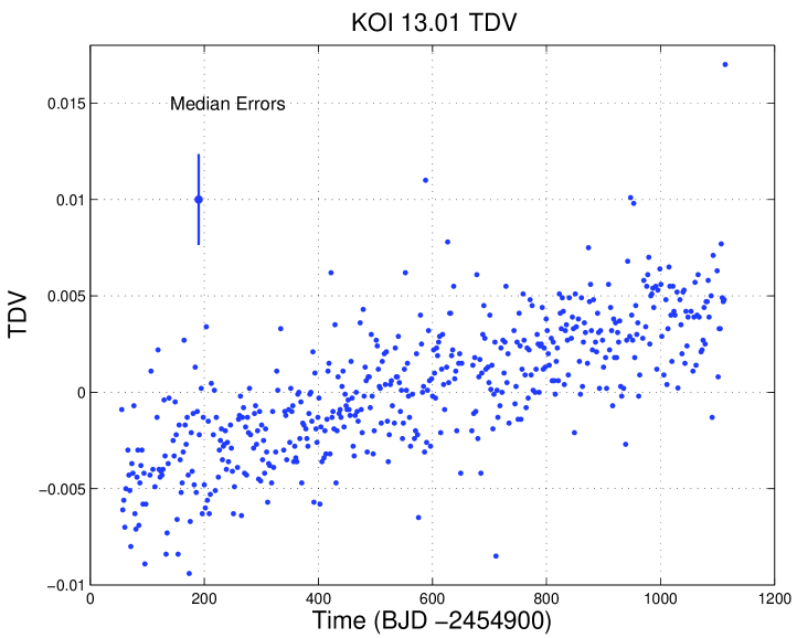
Although the main focus of this paper was the TTVs of the KOIs, we opted to vary the three parameters of the template simultaneously for KOIs with high enough SNRs, because we found a few KOIs for which the transit duration or depth did vary significantly, either because of physical processes, or as a result of some observational effects. One example is KOI-13, for which Szabó et al. (2012) have found some indications for a long-term variation of the impact parameter, equivalent to detecting variation of the transit duration. Our analysis, now based on twelve quarters, confirms the result of Szabó et al. (2012), and is presented in Figure 1. One can see the highly significant linear duration variation of KOI-13, which amounts to $\sim 1\%$ peak-to-peak modulation over the entire data span. For such cases the simultaneous analysis of timing, duration and depth is an advantage, and, in principle, can yield better timing of each transit.

Figure 1: The TDV (duration variation) of KOI-13.01. Each point represents our best estimate for the deviation of the transit duration from its averaged value, in units of the averaged duration. A typical error is included in the figure.

However, for low-SNR transits, minimizing the $\chi^{2}$ function with respect to the three parameters simultaneously could yield a completely erroneous result, based on some accidental local minimum in a noisy $\chi^{2}$ surface. In fact, for systems with even lower SNR, fitting the timing alone could yield misleading minima. We therefore divided the KOIs into three groups, according to their typical SNR for a single transit, defined as:

$${\rm SNR}=\frac{\delta}{\sigma}\sqrt{N}\ ,$$ (1)

where $\delta$ is the relative transit depth, $\sigma$ is the relative uncertainty per point, derived from the scatter of the light curve outside the transit, and $N$ is the averaged number of points per single transit. For each KOI we derived the median of its transit SNRs.

We considered three classes of KOIs:

• ${\rm SNR}<2.5$ — This class included $340$ KOIs. We did not perform any analysis for objects of this class, due to the poor SNR.

• $2.5<{\rm SNR}<10$ — This class included $1239$ KOIs, for which we have calculated TTs, while fixing the transit duration and depth, derived from the best-fit model.

• $SNR>10$ — For the 721 KOIs in this class, we derived simultaneously the transit timing, duration and depth.

2.1 Transit model

Our default choice for the transit templates was the Mandel & Agol (2002) model, which we derived for each KOI’s folded light curve through a $\chi^{2}$ minimization. However, since some transits showed slight asymmetries, e.g., KOI-13 (Szabó et al., 2011; Mazeh et al., 2012), and other transits had SNR values which were too low for a convincing Mandel-Agol fit, we used two additional models as possible templates: ”Legendre-based” and ”Fermi-based” models, which are described below. We computed these three models for each KOI, and chose the model with the lowest $\chi^{2}$ value as the transit template. However, due to the astrophysical basis of the Mandel-Agol model — in contrast to the other two which were merely mathematical heuristics — we preferred the Mandel-Agol model whenever it gave a good enough fit. Hence, we chose the Mandel-Agol model also in cases where its r.m.s. exceeded the r.m.s. of the other two models by up to 5%.

Below we provide a few details about the three models:

• We used our own code to fit the Mandel & Agol (2002) model, with a quadratic limb-darkening law, using coefficients that we interpolated from Claret & Bloemen (2011) tables, assuming $log\ g=4$, Solar metallicity, and Kepler KIC temperature (Brown et al., 2011).

• The Legendre-based model had the form:

  $$F\left(\tau\right)=\sum_{k=1}^{N_{1}}A_{k}L^{k}\left(\tau\right)+\sum_{k=1}^{N_{2}}S_{k}\,sin\left(\pi k\tau\right)+\sum_{k=1}^{N_{3}}C_{k}\,cos\left(\frac{\pi}{2}k\tau\right)\,,$$ (2)

  where $L^{k}$ was the Legendre polynomial of order $k$, $\tau$ was the normalized phase of the transit, such that at the beginning of ingress $\tau\left(t_{1}\right)=-1$, and at the end of egress $\tau\left(t_{4}\right)=+1$, $A_{k},S_{k}$ and $C_{k}$ were linear parameters found analytically, and $N_{1}=N_{2}=N_{3}=10$ were the maximum orders we allowed for each function. We optimized the model by varying the phases of $t_{1}$ and $t_{4}$ within the orbital period. We avoided local bumps in the model by reducing its three orders ($N_{1}$, $N_{2}$ and $N_{3}$) separately and by using linear fits to overcome local changes in convexity.

• The Fermi-based model had the form:

  $$F\left(\tau\right)=1+M\left[\frac{1}{e^{\left(\tau+\varphi+\mu\right)/s}+1}+\frac{1}{e^{\left(\tau+\varphi-\mu\right)/s}+1}-1\right],$$ (3)

  where $\tau$ was the phase of the transit, as for the Legendre model, and $\varphi$, $s$, $\mu$ and $M$ were free parameters, standing for the transit phase, ingress and egress steepness, width and depth of the transit. In order to obtain a more ”transit-like” shape, we replaced the points at the bottom part of the transit with a parabola, with its width as another free parameter, under the constraint that the resulting function and its first derivative were both continuous.

For most KOIs the pipeline selected the Mandel & Agol (2002) model (1829 KOIs). It chose the Legendre-based model when there was a significant asymmetry in the folded light curve of the transit (87 KOIs), and the Fermi-based one only when the SNR of the folded light curve was low (44 KOIs).

2.2 Finding the timing, duration and depth of each transit and their uncertainties

We analyzed each transit after fitting a polynomial to the light curve on the two sides of the transit, in order to remove stellar and instrumental long-term photometric variations during the transit.

We derived the timing, and when appropriate the duration and depth, of each transit by minimizing the standard $\chi^{2}$ function using the MATLAB FMINSEARCH function, based on the Nelder-Mead Simplex method (Lagarais, Reeds & Wright, 1998), assuming each measurement had the same error. Our pipeline then made sure that the $\chi^{2}$-minimum found was indeed the global minimum by an automated grid search over the parameter space. We then used the $\mathcal{F}$-test to compare the transit model with the timing (and duration and depth when appropriate) found against a constant flux assumption (no transit at all), and rejected all transits with an $\mathcal{F}$-test False Alarm Probability (=FAP) larger than 0.025. For these cases, the transit timing table quotes no timing (nor duration and depth).

We estimated the errors of the three quantities from the inverted Hessian matrix, calculated at the minimum. The error of each individual Kepler measurement was based on the scatter of the light curve around the polynomial fit before and after each transit. When the Hessian matrix turned out to be singular, we assigned an error that was equal to the median of the other errors derived for the KOI in question. Whenever that was the case we marked the error with an asterisk in the table of transit timings.

For each KOI, we ignored outlying timing, duration and depth values when their corresponding O-C values were too different from the other O-Cs of that KOI, or their error estimate was too large. Usually, a large error meant that some photometric measurements during that transit were erroneous. We rejected outliers based on both global and local mean and scatter. A value was considered an outlier if it deviated from the mean by more than five times the scatter of the series, defined as 1.4826 times its Median Absolute Deviation (MAD), plus three times its own error.

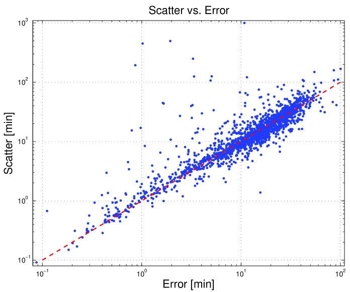
In order to check the obtained uncertainties for the transit timings, we computed for each KOI the scatter of its O-C values, $s_{\rm O-C}$, and compared it with its typical error, derived for each KOI by the median of its timing uncertainties — $\overline{\sigma}_{\rm TT}$. We expect these two values to be similar for systems with no significant TTV. This is indeed the case, as can be seen in Figure 2. The KOIs with O-C scatter larger than their uncertainties are those with significant TTVs.

Figure 2: The scatter of the derived O-C timings as a function of their typical uncertainty for all $1960$ KOIs.

Another approach to check our error estimate is to compare the typical derived error of a KOI with the SNR of its transit. One can expect the timing precision to improve with higher SNR. In order to see whether this is really the case, Figure 3 shows the median error, $\overline{\sigma}_{\rm TT}$, versus the median SNR of that KOI, presenting a tight correlation over the whole range of SNR, which goes from 2.5 to 1000. The plot is consistent with the simple relation

$$\overline{\sigma}_{\rm TT}\simeq\frac{100}{{\rm SNR}}\ ,$$ (4)

which is also plotted in the figure.

Figure 3: Typical transit timing uncertainty as a function of the typical SNR of a single transit for each KOI. The dashed red line represents $\overline{\sigma}_{\rm TT}=100/$SNR

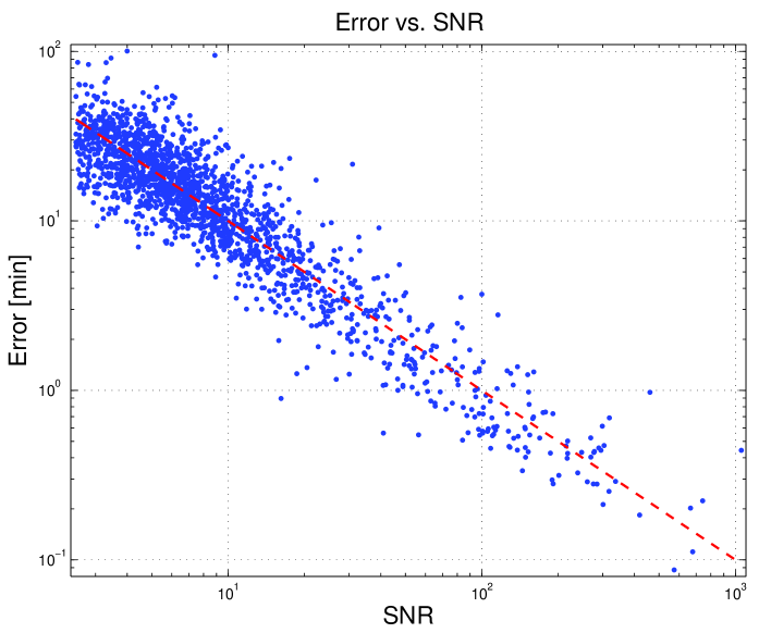
The last two figures suggest that our error estimate is realistic.

2.3 The catalog

We present our results in two tables, available at ftp://wise-ftp.tau.ac.il/pub/tauttv/TTV. Table 1 lists the modified ephemerides of the KOIs, based on our analysis, together with the durations and depths of their transits, derived from the folded light curve. The transit duration is quoted as a fraction of the orbital period and the depth in units of the stellar intensity outside the transit. Table 2 lists our derived O-Cs, relative to our modified ephemerides, for 167934 transits of 1960 KOIs with ${\rm SNR}>2.5$. Of those, duration and depth changes, in units of the transit model duration and depth, are given for $62802$ transits of 721 KOIs with ${\rm SNR}>10$.

Table 1: Linear ephemerides of the KOI transits, together with their durations and depths

KOI	T0	Period	Duration	Depth	SNR
	[d]	[d]

$1.01$	$55.762538$	$2.47061337$	$0.0315$	$0.01419$	$573.4$
	$\pm 0.000009$	$\pm 0.00000004$
$2.01$	$54.357833$	$2.20473534$	$0.0764$	$0.00669$	$317.3$
	$\pm 0.000019$	$\pm 0.00000006$
$3.01$	$57.812640$	$4.88780191$	$0.0222$	$0.00433$	$300.8$
	$\pm 0.000074$	$\pm 0.00000058$
$4.01$	$90.526015$	$3.84937129$	$0.0298$	$0.00132$	$31.1$
	$\pm 0.000315$	$\pm 0.00000186$
$5.01$	$65.973089$	$4.78032914$	$0.0186$	$0.00098$	$34.4$
	$\pm 0.000198$	$\pm 0.00000144$
$7.01$	$56.611453$	$3.21366766$	$0.0552$	$0.00074$	$24.1$
	$\pm 0.000359$	$\pm 0.00000184$
$10.01$	$54.118640$	$3.52249863$	$0.0391$	$0.00937$	$127.4$
	$\pm 0.000057$	$\pm 0.00000031$
$12.01$	$79.595944$	$17.85521101$	$0.0172$	$0.00917$	$318.6$
	$\pm 0.000413$	$\pm 0.00001133$
$13.01$	$53.565019$	$1.76358759$	$0.0790$	$0.00460$	$419.1$
	$\pm 0.000011$	$\pm 0.00000003$
$17.01$	$54.485821$	$3.23469919$	$0.0477$	$0.01078$	$239.0$
	$\pm 0.000034$	$\pm 0.00000018$

Table 2: O-C, duration (TDV) and depth (TPV) changes of the transits

n	t${}_{n}\tablenotemark{b}$	O-Cn	$\sigma_{n}$	TDVn	$\sigma_{n}$	TPVn	$\sigma_{n}$
	[d]	[min]	[min]
$0$	$55.7625$	$-0.057$	$0.085$	$0.0009$	$0.003$	$-0.0048$	$0.0028$
$1$	$58.2332$	$0.054$	$0.074$	$-0.0015$	$0.0023$	$-0.0067$	$0.0023$
$2$	$60.7038$	$-0.042$	$0.098$	$0.0019$	$0.0028$	$-0.01$	$0.003$
$3$	$63.1744$	$0.06$	$0.12$	$-0.0049$	$0.0033$	$-0.0018$	$0.0036$
$5$	$68.1156$	$-0.003$	$0.095$	$-0.0015$	$0.0026$	$-0.0006$	$0.0028$
$6$	$70.5862$	$0.07$	$0.11$	$-0.0028$	$0.0034$	$-0.0009$	$0.0035$
$7$	$73.0568$	$0.159$	$0.067$	$0.0185$	$0.0021$	$-0.0296$	$0.0021$
$8$	$75.5274$	$0.19$	$0.11$	$0.0039$	$0.0039$	$-0.0016$	$0.0035$
$9$	$77.9981$	$0.06$	$0.11$	$-0.0086$	$0.0042$	$0.0064$	$0.0038$
$10$	$80.4687$	$-0.074$	$0.072$	$0.0037$	$0.0026$	$-0.0108$	$0.0024$

3 Identifying KOIs with significant TTVs

As the main focus of this study is the TTVs of the KOIs, the next sections concentrate on the analysis of the derived O-Cs. Analyses of duration (TDV) and depth (TPV) variations are deferred to a later paper.

In order to identify KOIs with significant TTVs, we computed a few statistics (see F11, F12 and S12) to characterize the scatter of the derived O-Cs. We obtained these statistics, listed in Table 3, only for $1897$ KOIs which had at least seven timing measurements.

• For each KOI, we list the scatter of the O-Cs, $s_{\rm O-C}$, which we defined as the median absolute deviation (MAD) of the O-C series, and $\overline{\sigma}_{\rm TT}$, their median error (see Figure 2 and the discussion there). High values of $s_{\rm O-C}$ relative to $\overline{\sigma}_{\rm TT}$ may indicate a significant TTV, especially because the MAD statistic is less sensitive to outliers than the r.m.s.

However, the derived ratio relies on our estimate of the timing error, which by itself depends on the estimated error and the nature of the noise of the Kepler measurements. Although Figure 2 and Figure 3 indicate that our error estimates are realistic, we are not sure how accurate the uncertainties for a given KOI are, because of the unknown contribution of the red noise in the Kepler data. Another drawback of the scatter/error ratio is its insensitivity to the order of the residuals. That is, any permutation of the residuals yields the same two values. However, as pointed out by F11 (see also Agol et al., 2005; Holman & Murray, 2005; Lithwick et al., 2012), the expected time scale of the dynamical interaction between planets is in most cases larger than the orbital period of the transiting planet. We therefore can assume long-term correlation in the planet’s O-Cs, if indeed the planet is subject to a dynamical perturbation.

We therefore do not rely solely on the $s_{\rm O-C}/\overline{\sigma}_{\rm TT}$ ratio, and add three statistics that can indicate long-term correlation of the O-Cs:

• The Lomb-Scargle (LS) periodogram (e.g., S12), which searched for a cosine-shape periodicity in the series of O-Cs. We identified the highest peak in the periodogram and assigned a false-alarm probability (FAP) to the existence of the associated periodicity in the data. This was done by calculating similar $10^{4}$ LS periodograms with different random permutations of the same O-Cs, and obtaining the highest peak in each of these periodograms. Table 3 quotes the estimated period and its FAP p-value.

• A long-term polynomial fit to the series of TTVs. A good polynomial fit usually indicates a long-term modulation with a time scale longer than the data span. We searched for a polynomial with a degree lower than four, chose the best fit and tested its significance with the $\mathcal{F}$-test (e.g., F11). Table 3 quotes the best polynomial fit and its FAP p-value.

• The ’alarm’ score $\mathcal{A}$ of Tamuz, Mazeh & North (2006), which is sensitive to the correlation between adjacent O-Cs. The value of $\mathcal{A}$ reflects the number of consecutive TTVs with the same sign, without assuming any functional shape of the modulation (see Tamuz, Mazeh & North (2006) for a detailed discussion). We calculated $\mathcal{A}$ relative to the assumption of no TTV. We assigned a false-alarm probability to the occurrence of the obtained score by calculating alarm scores for $10^{4}$ different random permutations of the same TTVs. Table 3 quotes the alarm score and its p-value.

Table 3 can be used to identify KOIs with significant TTVs of various time scales.

Table 3: Statistical parameters of the O-Cs series of Kepler KOIs

KOI	$\overline{\sigma}_{\rm TT}\tablenotemark{a}$	$S_{\rm O-C}\tablenotemark{b}$	LS	LS	p-LS	$\mathcal{A}$	p-$\mathcal{A}$	Pol.	p-$\mathcal{F}$
			Period	Peak				Deg.
	[min]	[min]	[d]		[log]		[log]		[log]
$1.01$	$0.09$	$0.09$	$195.56$	$6.05$	$-0.2$	$0.282$	$-1.3$	$1$	$-0.3$
$2.01$	$0.25$	$0.24$	$21.55$	$12.72$	$-2.7$	$0.121$	$-1.0$	$2$	$-0.3$
$3.01$	$0.21$	$0.31$	$73.21$	$4.84$	$-0.1$	$0.239$	$-1.0$	$3$	$-0.3$
$4.01$	$2.22$	$2.79$	$11.96$	$5.82$	$-0.2$	$-0.241$	$-0.2$	$1$	$-0.3$
$5.01$	$1.66$	$1.58$	$44.69$	$6.44$	$-0.5$	$0.223$	$-1.1$	$1$	$-0.3$
$7.01$	$3.59$	$3.37$	$6.89$	$4.79$	$0.0$	$-0.144$	$-0.2$	$1$	$-0.3$
$10.01$	$0.57$	$0.56$	$16.92$	$6.68$	$-0.5$	$-0.256$	$-0.1$	$2$	$-0.3$
$12.01$	$0.69$	$1.33$	$849.19$	$8.84$	$-2.4$	$2.295$	$-3.5$	$2$	$-0.5$
$13.01$	$0.18$	$0.15$	$5.72$	$15.44$	$-4.0$	$-0.082$	$-0.4$	$2$	$-0.3$
$17.01$	$0.33$	$0.37$	$10.89$	$5.97$	$-0.2$	$0.692$	$-2.2$	$1$	$-0.3$

4 KOIs with significant TTVs

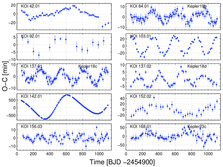
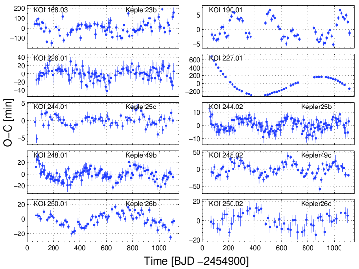
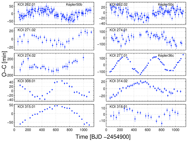
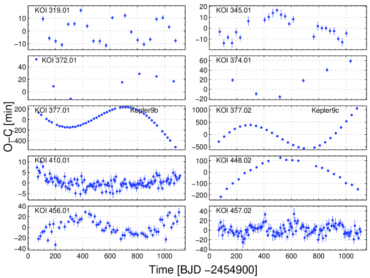
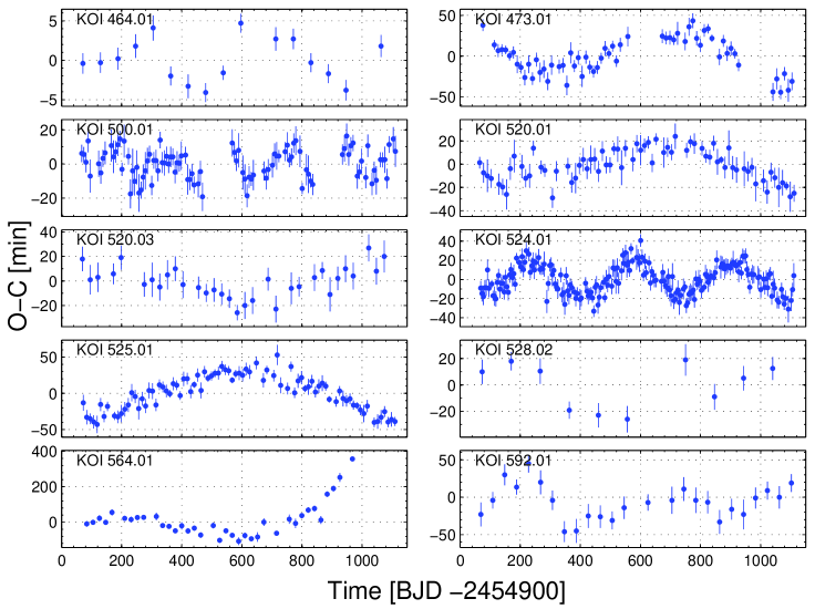
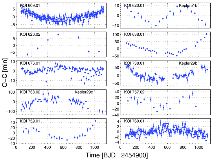
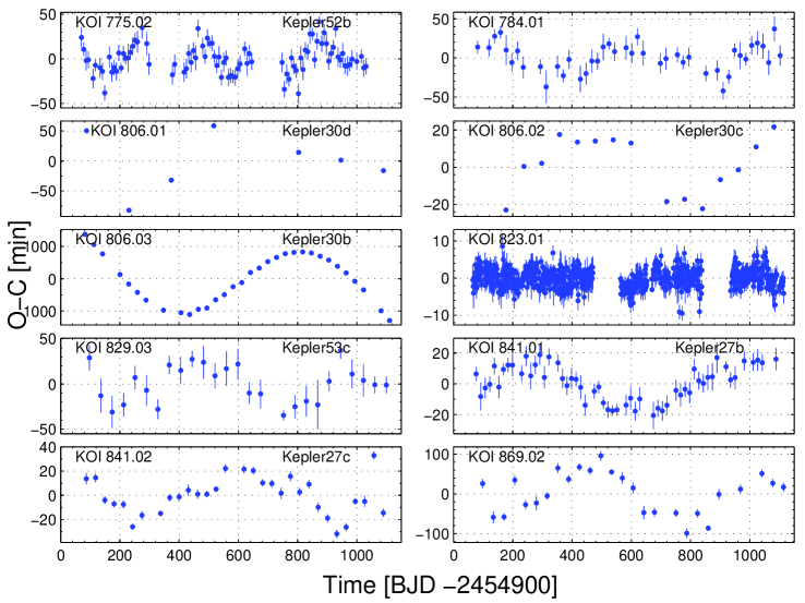
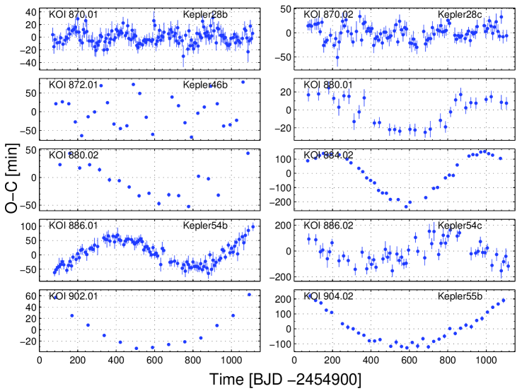
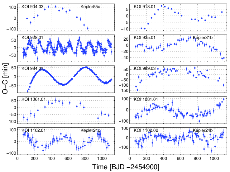
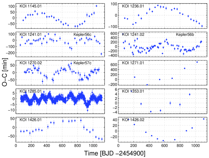
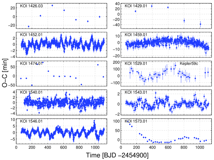
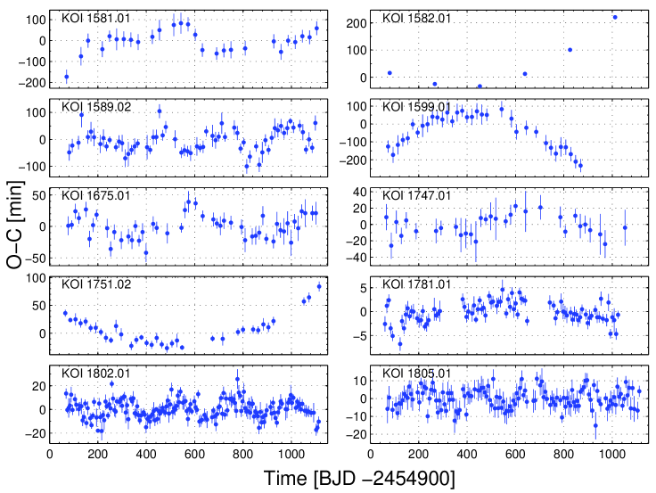
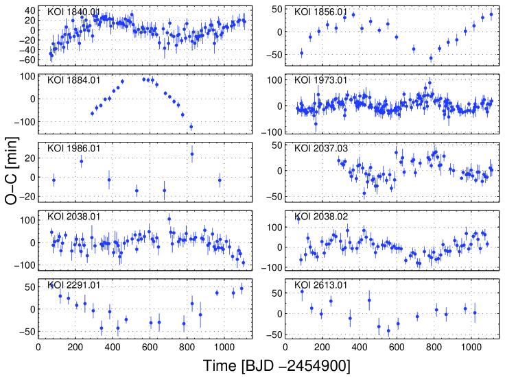
In this section we single out 130 systems with significant TTVs, either because they have large scatter ($s_{\rm O-C}$ /$\overline{\sigma}_{\rm TT}>15$), display a periodic modulation (LS FAP lower than $3\times$10^-4) or show a parabolic trend (see Table 3). Figures 4–16 display the O-Cs of these systems, and Table 4 summarizes their variability features. Eight KOIs — 94.02, 341.01, 1376.01, 1458.01, 1814.01, 1815.01, 2276.01 and 2631.01 are not included because they do not look significantly variable, even though they have passed one of these criteria.

Eighty five of the $130$ KOIs showed some periodicity, with time scales ranging from $100$ to $1000$ days and amplitudes of $1$–$1000$ minutes. For each of these $85$ systems, we derived a fit to the O-Cs (not plotted but given in the table), composed of a straight line, which could present a correction to the orbital period of the transiting planet, together with a cosine function with the best-found period and phase. Table 4 lists the period and its error for $48$ KOIs. For $37$ systems the period found was too long or the fit was not good enough and we could not derive its uncertainty. In those cases, the period listed is just an approximation. In one special case — KOI-142.01, we fitted a straight line with two different cosine functions.

For $39$ KOIs, the O-C series did not exhibit a maximum and a minimum, and therefore we have not fitted a cosine function to the data. This probably meant that the time scale of the modulation was longer than the time span of the data. In those cases, we fitted the O-Cs with a long-term parabola only, and added a note in Table 4.

For six systems — KOI-1285.01, 1452.01, 1474.01, 1540.01, 1543.01 and 1546.01, neither a cosine function nor a parabola could be fitted, but the O-Cs looked nevertheless significant (see Section 6 for s short discussion of all six KOIs).

Table 4 lists the KOI number, the orbital period of the transiting planet and the model we used, either a Cosine function, ”C”, or a polynomial ”P”. For a Cosine fit, we list the TTV period and its error, when available, and the amplitude. The next column gives the scatter of the residuals relative to the found fit (which is not plotted). We also list the number of TTV measurements, the multiplicity of the of KOI and references to previous studies, when available. In Section 6 we briefly comment on some of the systems listed here. These systems are marked by an asterisk in the table.

Table 4: KOIs with significant TTV

KOI	Period	Model	Period	$\sigma_{P}\tablenotemark{d}$	Amp	$\sigma_{A}\tablenotemark{f}$	Res	$N$	Multi-	Ref.
	[d]		[d]	[d]	[min]	[min]	[min]		plicity
$42.01$	$17.83$	C	$960$	$\cdots$	$13.91$	$0.91$	$3.3$	$53$	$1$
$84.01$	$9.29$	C	$300$	$31$	$4.54$	$0.39$	$2.7$	$104$	$1$	Kepler19b
$92.01$	$65.70$	C	$519$	$84$	$4.42$	$0.76$	$2$	$14$	$1$
$103.01$	$14.91$	C	$261$	$13$	$26.14$	$0.83$	$4.5$	$61$	$1$
$137.01$	$7.64$	C	$268$	$21$	$5.38$	$0.26$	$1.7$	$120$	$3$	Kepler18c
$137.02$	$14.86$	C	$267$	$26$	$4.11$	$0.31$	$1.2$	$61$	$3$	Kepler18d
$\tablenotemark{*}142.01$	$10.95$	C	$618$	$58$	$664$	$15$	$96$	$88$	$1$
			$339$	$20$	$111$	$5$	$25$
$152.02$	$27.40$	C	$870$	$\cdots$	$20.8$	$2.4$	$7.7$	$36$	$3$
$156.03$	$11.78$	C	$167$	$12$	$3.02$	$0.48$	$2.5$	$81$	$3$
$168.01$	$10.74$	C	$474$	$89$	$19.8$	$2.2$	$13$	$82$	$3$	Kepler23c
$168.03$	$7.11$	C	$478$	$90$	$52$	$8.2$	$38$	$88$	$3$	Kepler23b
$\tablenotemark{*}190.01$	$12.26$	C	$267$	$22$	$4.31$	$0.31$	$1.6$	$65$	$1$
$226.01$	$8.31$	C	$610$	$210$	$8.9$	$1.8$	$12$	$105$	$1$
$227.01$	$17.70$	C	$1000$	$\cdots$	$397.4$	$9.5$	$29$	$44$	$1$
$244.01$	$12.72$	C	$316$	$39$	$1.24$	$0.22$	$1.2$	$71$	$2$	Kepler25c
$244.02$	$6.24$	C	$340$	$45$	$4.13$	$0.39$	$3$	$145$	$2$	Kepler25b
$248.01$	$7.20$	C	$384$	$58$	$9.51$	$0.92$	$6.2$	$125$	$4$	Kepler49b
$248.02$	$10.91$	C	$370$	$54$	$17.7$	$1.8$	$11$	$83$	$4$	Kepler49c
$250.01$	$12.28$	C	$750$	$\cdots$	$10.35$	$0.98$	$5.9$	$76$	$4$	Kepler26b
$250.02$	$17.25$	C	$800$	$\cdots$	$7.7$	$1.3$	$5.9$	$50$	$4$	Kepler26c
$262.01$	$7.81$	C	$750$	$\cdots$	$26.4$	$2.2$	$15$	$103$	$2$	Kepler50b
$262.02$	$9.38$	C	$880$	$\cdots$	$15.5$	$1.6$	$9.9$	$92$	$2$	Kepler50c
$271.02$	$29.39$	C	$880$	$\cdots$	$12.1$	$1.6$	$4.2$	$29$	$2$
$274.01$	$15.09$	P	$\cdots$	$\cdots$	$\cdots$	$\cdots$	$45$	$48$	$2$
$274.02$	$22.80$	P	$\cdots$	$\cdots$	$\cdots$	$\cdots$	$45$	$29$	$2$
$277.01$	$16.23$	C	$440$	$29$	$116.6$	$3.1$	$15$	$54$	$1$	Kepler36c
$308.01$	$35.60$	C	$623$	$79$	$34.4$	$2.1$	$5.7$	$27$	$1$
$314.02$	$23.09$	P	$\cdots$	$\cdots$	$\cdots$	$\cdots$	$5.3$	$41$	$3$
$315.01$	$35.59$	P	$\cdots$	$\cdots$	$\cdots$	$\cdots$	$8.5$	$27$	$1$
$318.01$	$38.58$	C	$690$	$\cdots$	$6.4$	$1.3$	$2.3$	$23$	$1$

Table 4: - continued

KOI	Period	Model	Period	$\sigma_{P}\tablenotemark{d}$	Amp	$\sigma_{A}\tablenotemark{f}$	Res	$N$	Multi-	Ref.
	[d]		[d]	[d]	[min]	[min]	[min]		plicity
$319.01$	$46.15$	C	$303$	$19$	$12.3$	$1.2$	$3.2$	$21$	$1$
$345.01$	$29.88$	P	$\cdots$	$\cdots$	$\cdots$	$\cdots$	$3$	$24$	$1$
$372.01$	$125.63$	C	$1000$	$\cdots$	$35.8$	$5.6$	$7.6$	$7$	$1$
$374.01$	$172.69$	P	$\cdots$	$\cdots$	$\cdots$	$\cdots$	$13$	$6$	$1$
$377.01$	$19.26$	C	$1000$	$\cdots$	$324.8$	$2$	$6.4$	$48$	$3$	Kepler9b
$377.02$	$38.88$	C	$1000$	$\cdots$	$764.9$	$4.5$	$6.3$	$26$	$3$	Kepler9c
$410.01$	$7.22$	P	$\cdots$	$\cdots$	$\cdots$	$\cdots$	$1.7$	$130$	$1$
$448.02$	$43.59$	P	$\cdots$	$\cdots$	$\cdots$	$\cdots$	$11$	$21$	$2$
$456.01$	$13.70$	C	$730$	$\cdots$	$16.6$	$1.5$	$9.3$	$69$	$2$
$457.02$	$7.06$	C	$281$	$36$	$8.5$	$1.1$	$7.4$	$128$	$2$
$464.01$	$58.36$	C	$451$	$77$	$3.16$	$0.7$	$1.4$	$16$	$2$
$473.01$	$12.71$	C	$860$	$\cdots$	$30.4$	$2.1$	$12$	$60$	$1$
$500.01$	$7.05$	C	$190$	$17$	$7.88$	$0.98$	$6.6$	$100$	$5$
$520.01$	$12.76$	P	$\cdots$	$\cdots$	$\cdots$	$\cdots$	$8.2$	$70$	$3$
$520.03$	$25.75$	P	$\cdots$	$\cdots$	$\cdots$	$\cdots$	$7.1$	$32$	$3$
$524.01$	$4.59$	C	$336$	$44$	$16.98$	$0.82$	$7.9$	$195$	$1$
$525.01$	$11.53$	P	$\cdots$	$\cdots$	$\cdots$	$\cdots$	$9.8$	$84$	$1$
$528.02$	$96.68$	P	$\cdots$	$\cdots$	$\cdots$	$\cdots$	$8$	$10$	$3$
$564.01$	$21.06$	C	$880$	$\cdots$	$120$	$11$	$24$	$37$	$2$
$592.01$	$39.75$	C	$449$	$73$	$24.4$	$4.6$	$12$	$25$	$1$
$\tablenotemark{*}609.01$	$4.40$	P	$\cdots$	$\cdots$	$\cdots$	$\cdots$	$1.4$	$207$	$1$
$620.01$	$45.16$	C	$760$	$\cdots$	$8.5$	$0.78$	$2.3$	$22$	$3$	Kepler51b
$620.02$	$130.18$	P	$\cdots$	$\cdots$	$\cdots$	$\cdots$	$1.2$	$7$	$3$
$638.01$	$23.64$	P	$\cdots$	$\cdots$	$\cdots$	$\cdots$	$8.7$	$32$	$2$
$676.01$	$7.97$	C	$690$	$\cdots$	$2.48$	$0.36$	$2$	$102$	$2$
$738.01$	$10.34$	P	$\cdots$	$\cdots$	$\cdots$	$\cdots$	$12$	$70$	$2$	Kepler29b
$738.02$	$13.29$	P	$\cdots$	$\cdots$	$\cdots$	$\cdots$	$19$	$50$	$2$	Kepler29c
$757.02$	$41.19$	P	$\cdots$	$\cdots$	$\cdots$	$\cdots$	$9.2$	$18$	$3$
$759.01$	$32.63$	P	$\cdots$	$\cdots$	$\cdots$	$\cdots$	$11$	$22$	$1$
$760.01$	$4.96$	P	$\cdots$	$\cdots$	$\cdots$	$\cdots$	$0.97$	$186$	$1$

Table 4: - continued

KOI	Period	Model	Period	$\sigma_{P}\tablenotemark{d}$	Amp	$\sigma_{A}\tablenotemark{f}$	Res	$N$	Multi-	Ref.
	[d]		[d]	[d]	[min]	[min]	[min]		plicity
$775.02$	$7.88$	C	$209$	$16$	$16.5$	$1.8$	$11$	$90$	$3$	Kepler52b
$784.01$	$19.27$	C	$486$	$88$	$18.4$	$2.8$	$14$	$42$	$2$
$806.01$	$143.21$	C	$400$	$\cdots$	$60$	$20$	$30$	$7$	$3$	Kepler30d
$806.02$	$60.32$	C	$750$	$\cdots$	$22.1$	$2.2$	$5.9$	$15$	$3$	Kepler30c
$806.03$	$29.37$	C	$930$	$120$	$1343.5$	$8.3$	$22$	$32$	$3$	Kepler30b
$\tablenotemark{*}823.01$	$1.03$	C	$184$	$12$	$0.85$	$0.13$	$2.4$	$676$	$1$
$829.03$	$38.56$	C	$501$	$77$	$25.2$	$4.7$	$11$	$26$	$3$	Kepler53c
$841.01$	$15.34$	C	$780$	$\cdots$	$14.8$	$1.1$	$4.6$	$55$	$2$	Kepler27b
$841.02$	$31.33$	C	$630$	$120$	$17.6$	$2.9$	$9.1$	$31$	$2$	Kepler27c
$869.02$	$36.28$	C	$600$	$140$	$65.2$	$7.7$	$27$	$26$	$4$
$870.01$	$5.91$	C	$231$	$23$	$8.74$	$1$	$7.9$	$149$	$2$	Kepler28b
$870.02$	$8.99$	C	$230$	$21$	$12.3$	$1.9$	$13$	$97$	$2$	Kepler28c
$872.01$	$33.60$	C	$191.1$	$9.2$	$54.6$	$5.3$	$19$	$28$	$2$	Kepler46b
$880.01$	$26.44$	C	$860$	$\cdots$	$20.5$	$1.8$	$4.5$	$31$	$4$
$880.02$	$51.53$	P	$\cdots$	$\cdots$	$\cdots$	$\cdots$	$13$	$18$	$4$
$884.02$	$20.49$	C	$837$	$98$	$175$	$3.7$	$14$	$36$	$3$
$886.01$	$8.01$	C	$860$	$\cdots$	$63.1$	$2.1$	$12$	$105$	$3$	Kepler54b
$886.02$	$12.07$	C	$800$	$\cdots$	$98$	$12$	$53$	$55$	$3$	Kepler54c
$902.01$	$83.92$	P	$\cdots$	$\cdots$	$\cdots$	$\cdots$	$1.2$	$13$	$1$
$904.02$	$27.96$	P	$\cdots$	$\cdots$	$\cdots$	$\cdots$	$18$	$35$	$5$	Kepler55b
$904.03$	$42.15$	P	$\cdots$	$\cdots$	$\cdots$	$\cdots$	$13$	$15$	$5$	Kepler55c
$918.01$	$39.64$	C	$950$	$\cdots$	$8.25$	$0.78$	$2.6$	$22$	$1$
$928.01$	$2.49$	C	$120$	$\cdots$	$30.4$	$1.5$	$17$	$273$	$1$
$\tablenotemark{*}935.01$	$20.86$	C	$1000$	$\cdots$	$25.3$	$1.9$	$5.8$	$44$	$4$	Kepler31b
$984.01$	$4.29$	C	$495$	$25$	$45.55$	$0.37$	$3.6$	$196$	$1$
$989.03$	$16.16$	P	$\cdots$	$\cdots$	$\cdots$	$\cdots$	$22$	$46$	$1$
$1061.01$	$41.81$	P	$\cdots$	$\cdots$	$\cdots$	$\cdots$	$17$	$19$	$1$
$1081.01$	$9.96$	C	$1000$	$\cdots$	$74.2$	$4.6$	$14$	$76$	$1$
$1102.01$	$12.33$	C	$421$	$54$	$50.8$	$4.2$	$21$	$58$	$2$	Kepler24c
$1102.02$	$8.15$	C	$434$	$62$	$29.7$	$4.2$	$23$	$92$	$2$	Kepler24b

Table 4: - continued

KOI	Period	Model	Period	$\sigma_{P}\tablenotemark{d}$	Amp	$\sigma_{A}\tablenotemark{f}$	Res	$N$	Multi-	Ref.
	[d]		[d]	[d]	[min]	[min]	[min]		plicity
$1145.01$	$30.59$	C	$950$	$\cdots$	$76.8$	$4.5$	$9.6$	$29$	$1$
$1236.01$	$35.74$	P	$\cdots$	$\cdots$	$\cdots$	$\cdots$	$22$	$25$	$2$
$1241.01$	$21.41$	C	$524$	$90$	$42$	$11$	$32$	$41$	$2$	Kepler56c
$1241.02$	$10.50$	C	$509$	$78$	$161$	$21$	$100$	$70$	$2$	Kepler56b
$1270.02$	$11.61$	C	$459$	$75$	$34.5$	$3.3$	$14$	$61$	$2$	Kepler57c
$1271.01$	$161.86$	P	$\cdots$	$\cdots$	$\cdots$	$\cdots$	$86$	$6$	$1$
$\tablenotemark{*}1285.01$	$0.94$	$\cdots$	$\cdots$	$\cdots$	$\cdots$	$\cdots$	$\cdots$	$998$	$1$
$1353.01$	$125.87$	P	$\cdots$	$\cdots$	$\cdots$	$\cdots$	$0.51$	$7$	$2$
$1426.01$	$38.87$	P	$\cdots$	$\cdots$	$\cdots$	$\cdots$	$17$	$23$	$3$
$1426.02$	$74.92$	C	$970$	$\cdots$	$36.3$	$4.2$	$6.8$	$10$	$3$
$1426.03$	$150.02$	C	$820$	$\cdots$	$22.4$	$2.3$	$1.3$	$7$	$3$
$1429.01$	$205.92$	P	$\cdots$	$\cdots$	$\cdots$	$\cdots$	$3.5$	$5$	$1$
$\tablenotemark{*}1452.01$	$1.15$	$\cdots$	$\cdots$	$\cdots$	$\cdots$	$\cdots$	$\cdots$	$801$	$1$
$1459.01$	$0.69$	P	$\cdots$	$\cdots$	$\cdots$	$\cdots$	$2.8$	$493$	$1$
$\tablenotemark{*}1474.01$	$69.73$	$\cdots$	$\cdots$	$\cdots$	$\cdots$	$\cdots$	$\cdots$	$14$	$1$
$1529.01$	$17.98$	C	$520$	$76$	$61.7$	$7.4$	$27$	$38$	$2$	Kepler59c
$\tablenotemark{*}1540.01$	$1.21$	$\cdots$	$\cdots$	$\cdots$	$\cdots$	$\cdots$	$\cdots$	$741$	$1$
$\tablenotemark{*}1543.01$	$3.96$	$\cdots$	$\cdots$	$\cdots$	$\cdots$	$\cdots$	$\cdots$	$231$	$1$
$\tablenotemark{*}1546.01$	$0.92$	$\cdots$	$\cdots$	$\cdots$	$\cdots$	$\cdots$	$\cdots$	$993$	$1$
$1573.01$	$24.81$	C	$990$	$\cdots$	$39$	$1.4$	$3.3$	$32$	$1$
$1581.01$	$29.54$	C	$1000$	$\cdots$	$90$	$13$	$26$	$27$	$1$
$1582.01$	$186.40$	P	$\cdots$	$\cdots$	$\cdots$	$\cdots$	$3.4$	$6$	$1$
$1589.02$	$12.88$	C	$268$	$24$	$37.4$	$4.9$	$24$	$65$	$5$
$1599.01$	$20.41$	P	$\cdots$	$\cdots$	$\cdots$	$\cdots$	$26$	$34$	$1$
$1675.01$	$14.62$	C	$510$	$110$	$17.7$	$2.8$	$11$	$50$	$1$
$1747.01$	$20.56$	C	$760$	$\cdots$	$14.3$	$2.5$	$8$	$31$	$1$
$1751.02$	$21.00$	P	$\cdots$	$\cdots$	$\cdots$	$\cdots$	$6.2$	$35$	$2$
$1781.01$	$7.83$	P	$\cdots$	$\cdots$	$\cdots$	$\cdots$	$1.4$	$86$	$2$
$1802.01$	$5.25$	C	$232$	$21$	$6.91$	$0.61$	$5.3$	$177$	$1$
$1805.01$	$6.94$	C	$226$	$25$	$3.72$	$0.58$	$4.4$	$135$	$3$

Table 4: - continued

KOI	Period	Model	Period	$\sigma_{P}\tablenotemark{d}$	Amp	$\sigma_{A}\tablenotemark{f}$	Res	$N$	Multi-	Ref.
	[d]		[d]	[d]	[min]	[min]	[min]		plicity
$1840.01$	$7.04$	C	$1000$	$\cdots$	$31.5$	$2.1$	$9.4$	$119$	$1$
$1856.01$	$46.30$	C	$850$	$\cdots$	$42.7$	$3.4$	$4.5$	$21$	$1$
$1884.01$	$23.12$	P	$\cdots$	$\cdots$	$\cdots$	$\cdots$	$8.7$	$18$	$2$
$1973.01$	$3.29$	C	$417$	$81$	$19.1$	$1.7$	$13$	$166$	$1$
$1986.01$	$148.46$	C	$594$	$81$	$19.3$	$5.1$	$4.5$	$7$	$1$
$2037.03$	$8.56$	C	$510$	$170$	$18.8$	$2.1$	$10$	$63$	$2$
$2038.01$	$8.31$	C	$1000$	$\cdots$	$39.5$	$6.2$	$21$	$76$	$4$
$2038.02$	$12.51$	C	$680$	$\cdots$	$41.3$	$5.3$	$27$	$71$	$4$
$2291.01$	$44.30$	P	$\cdots$	$\cdots$	$\cdots$	$\cdots$	$11$	$18$	$1$
$2613.01$	$51.58$	P	$\cdots$	$\cdots$	$\cdots$	$\cdots$	$19$	$14$	$1$

Figure 4: KOIs with significant TTVs.

Figure 5: KOIs with significant TTVs.

Figure 6: KOIs with significant TTVs.

Figure 7: KOIs with significant TTVs.

Figure 8: KOIs with significant TTVs.

Figure 9: KOIs with significant TTVs.

Figure 10: KOIs with significant TTVs.

Figure 11: KOIs with significant TTVs.

Figure 12: KOIs with significant TTVs.

Figure 13: KOIs with significant TTVs.

Figure 14: KOIs with significant TTVs.

Figure 15: KOIs with significant TTVs.

Figure 16: KOIs with significant TTVs.

5 KOIs with short-period TTV

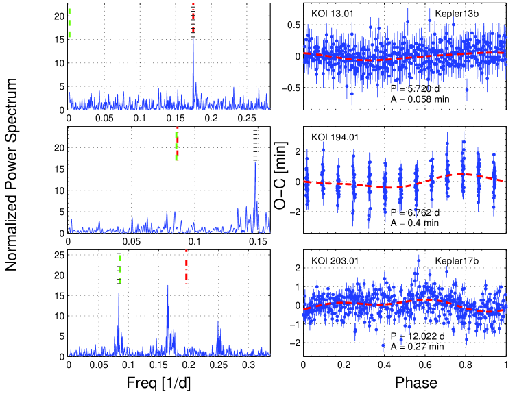
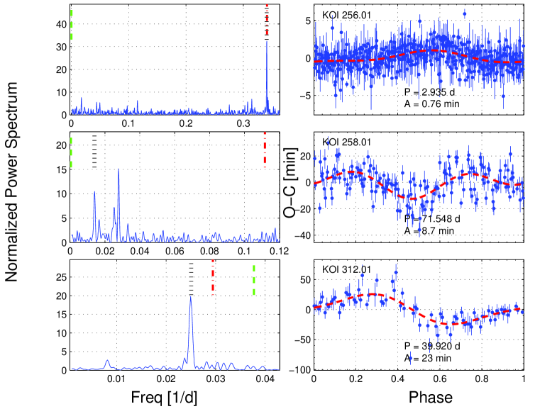
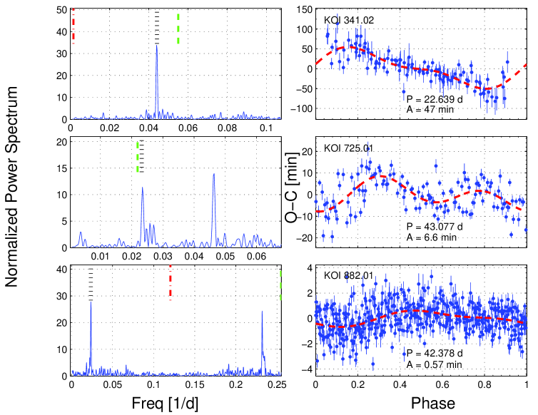
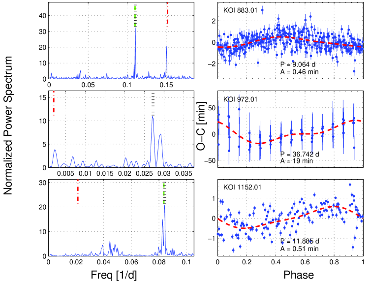
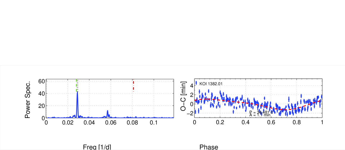
Our LS analysis of the O-Cs yielded also $13$ systems with highly significant short-period TTV modulations, in the range of 3 to 72 days. They were found using the same criterion as the one used in Section 4 — LS peak with FAP lower than 3$\times$10^-4. The modulation amplitudes were relatively small, in the range of $0.06-46$ minutes, and their detection was possible only because of the modulation periodicity and the long time span of the data. Figures 17–21 show the LS periodograms and the phase-folded O-Cs of the $13$ systems, where one can see the prominent peaks of the periodograms. Table 5 lists the periods and amplitudes found. The table includes references to Section 6, where we briefly comment on these systems.

As pointed out by Szabó et al. (2013, hereafter Sz13), not all detected short-period modulations are due to physical TTVs. An apparent TTV periodicity can be induced either by the long-cadence sampling of Kepler, or by an interference with a periodic stellar activity.

The finite sampling rate of the observations may cause a shift in the orbital phases of the observations during a transit, inducing an apparent shift of the derived timing of that transit. This can evoke a periodic TTV, with a period of

$$P_{\rm induced}=\frac{P_{\rm orb}}{\frac{P_{\rm orb}}{P_{\rm samp}}-\lfloor\frac{P_{\rm orb}}{P_{\rm samp}}\rfloor}\ ,$$ (5)

where $P_{\rm orb}$ is the orbital period, $P_{\rm samp}$ is the sampling cadence and $\lfloor x\rfloor$ is the floor of $x$ (Sz13). Note that the induced periodicity is observed with ”sampling” intervals equal to the planetary orbit, and therefore the relevant Nyquist frequency is $1/(2P_{\rm orb})$. If the induced frequency is larger, we will detect one of its aliases. We found two cases which suggested that the O-Cs included such effect (see below).

The other effect is due to the stellar spot activity, which modulates the stellar intensity with the stellar rotational period. Spot crossing (e.g., Sanchis-Ojeda et al., 2012) during a transit, or a slope of the stellar brightness during a transit, can cause a shift in the derived transit timing, inducing an apparent O-C periodicity with the stellar rotational period. In fact, $12$ out of the $13$ systems with short periodic modulation showed a high level of stellar activity, and we had to check whether the detected TTV periodicity was due to that activity.

To find the frequency of the presumed sampling-induced periodicity, we used for each KOI its $P_{\rm orb}$ from Table 1, and the pertinent $P_{\rm samp}$. This was about 29.424 minutes for the long cadence, the exact value taken to be the median of the differences of the observed timings of that KOI. We searched for stellar spot periodicity using the autocorrelation technique (e.g., McQuillan, Aigrain & Mazeh, 2013), and, if present, checked whether its frequency, or one of its aliases, was equal to the TTV frequency. We mark the pertinent frequencies in Figures 17–21.

Table 5: KOIs with significant short-period TTVs

KOI	Period	Period	$\sigma_{P}\tablenotemark{c}$	Amp	$\sigma_{A}\tablenotemark{e}$	Res	$N$	Multi-	Ref.
	[d]	[d]	[d]	[min]	[min]	[min]		plicity
$\tablenotemark{*}13.01$	$1.76$	$5.72$	$0.015$	$0.0578$	$\par 0.0094$	$0.15$	$520$	$1$	Kepler13b
$\tablenotemark{*}194.01$	$3.12$	$6.762$	$0.016\par$	$0.405$	$\par 0.06$	$0.71$	$293$	$1$
$\tablenotemark{*}203.01$	$1.49$	$12.022$	$\par 0.051$	$0.271$	$0.034$	$0.49$	$505$	$1$	Kepler17b
$\tablenotemark{*}256.01$	$1.38$	$2.9353$	$\par 0.0043$	$0.765$	$0.077$	$1.2$	$519$	$1$
$\tablenotemark{*}258.01$	$4.16$	$71.5$	$1.5$	$8.75$	$\par 0.79$	$9.1$	$174$	$1$
$\tablenotemark{*}312.01$	$11.58$	$39.92$	$0.48\par$	$23.4$	$\par 2$	$11$	$78$	$2$
$341.02$	$4.70$	$22.64$	$0.15$	$46.5$	$\par 2.7$	$17$	$112$	$2$
$\tablenotemark{*}725.01$	$7.30$	$43.08$	$0.56\par$	$6.59$	$\par 0.59$	$5.8$	$132$	$1$
$\tablenotemark{*}882.01$	$1.96$	$42.38$	$0.63\par$	$0.571$	$\par 0.068$	$1.1$	$484$	$1$
$\tablenotemark{*}883.01$	$2.69$	$9.064$	$0.045\par$	$0.457$	$\par 0.048$	$0.58$	$354$	$1$
$972.01$	$13.12$	$36.74$	$0.34$	$19$	$\par 1.9$	$9.8$	$69$	$1$
$\tablenotemark{*}1152.01$	$4.72$	$11.885$	$\par 0.049$	$0.509$	$0.063$	$0.43$	$148$	$1$
$\tablenotemark{*}1382.01$	$4.20$	$34.48$	$0.66\par$	$1.096$	$\par 0.079$	$0.8$	$201$	$1$

Figure 17: The KOIs with short-period TTVs. For each KOI, the plot shows the LS periodogram and the phase-folded O-Cs. The dotted black line represents the folding period, the dashed green line the stellar activity frequency or one of its aliases, if present in the stellar light curve, and the dash-dotted red line the frequency induced by the sampling. The phase-folded light-curve panels include a two-harmonic fit.

Figure 18: The KOIs with short-period TTVs. For each KOI, the LS periodogram and the phase-folded O-Cs are plotted (see Figure 17 for details).

Figure 19: The KOIs with short-period TTVs. For each KOI, the LS periodogram and the phase-folded O-Cs are plotted (see Figure 17 for details).

Figure 20: The KOIs with short-period TTVs. For each KOI, the LS periodogram and the phase-folded O-Cs are plotted (see Figure 17 for details).

Figure 21: The KOIs with short-period TTVs. For each KOI, the LS periodogram and the phase-folded O-Cs are plotted (see Figure 17 for details).

6 Comments on Individual Systems

In this section we comment on a few KOIs from Tables 4–5. In particular, we phase-folded the light curves of all $143$ systems with their orbital period, and searched for a secondary dip. For eleven systems we found a significant secondary dip, in most cases at phase $\sim 0.5$, which we interpreted as either an eclipse of a secondary star, or a planetary occultation. We also point out any periodic TTV modulation that could have been induced either by the long cadence sampling or by the stellar spot periodic activity. Some of these systems were analyzed in a similar way by Sz13, who used six quarters of Kepler data to look for TTV periodicity.

• KOI-$13.01$ (Figure 17): The O-Cs LS periodogram displays a prominent peak, corresponding to the induced sampling frequency. The folded light curve displays a shallow occultation.

• KOI-$142.01$ (Figure 4): The TTV modulation has one of the largest amplitudes in the sample. One cosine function was not enough to model the modulation, and therefoe the O-Cs include at least two different frequencies. This might be the result of some non-linear effect of the dynamical interaction. Nesvorný et al. (2013) derived the parameters of the unseen planet causing this TTV.

• KOI-$190.01$ (Figure 5): This system is probably an eclipsing binary (=EB) orbiting a third distant star, causing the light time travel (LITE) effect (Santerne et al., 2012).

• KOI-$194.01$ (Figure 17): The folded light curve displays a shallow occultation.

• KOI-$203.01$ (Figure 17): The TTV LS periodogram displays two prominent peaks. The higher frequency is the first harmonic of the other. The lower-peak frequency coincides with the stellar rotation, which has a modulation with a period of $12.05$ day. Sz13 reached the same conclusion.

• KOI-$256.01$ (Figure 18): The O-C LS periodogram displays a prominent peak, corresponding to the induced sampling frequency. Sz13 found a $41.8$ day period in the TTV.

• KOI-$258.01$ (Figure 18): The folded light curve reveals a dip around phase $0.5$, probably a secondary eclipse. Therefore the system is probably an EB. The star has a significantly high level of activity, probably due to stellar pulsations. The O-C LS periodogram displays two prominent peaks. The higher frequency is the first harmonic of the other.

• KOI-$312.01$ (Figure 18): The autocorrelation of the stellar photometry reveals a weak but stable modulation with a short period of $0.17073$ day. The green line in the figure is an alias of this frequency.

• KOI-$341.01$ : The orbital period used in our analysis is half the one published in B12. This KOI does not have a significant TTV and we do not include it in our tables.

• KOI-$609.01$ (Figure 9): The folded light curve displays a shallow occultation. Santerne et al. (2012) found it to be an EB.

• KOI-$725.01$ (Figure 19): The folded light curve displays a shallow occultation. The stellar photometry shows pulsations with a period of $8.58$ day. The O-C LS periodogram displays two prominent peaks. The higher frequency is the first harmonic of the other.

• KOI-$823.01$ (Figure 10): The folded light curve displays a relatively deep occultation. Sz13 found it to be a multi-periodic candidate.

• KOI-$882.01$ (Figure 20): The photometry displays strong stellar pulsations with a frequency of $3.921$ day, very close to twice the orbital period. The second peak in the periodogram is an alias of the first one, relative to the pulsation Nyquist frequency. Sz13 found the same TTV periodicity, with a noisier periodogram.

• KOI-$883.01$ (Figure 20): The O-C LS periodogram displays two prominent peaks. The higher one coincides with the stellar rotation, with a period of $9.02$ day, and the smaller one with the induced sampling frequency. Sz13 reached the same conclusion.

• KOI-$928.01$ (Figure 12): The orbital period is probably twice the one published by B12. This system is probably an EB orbiting a third distant star, causing a LITE effect (Steffen et al., 2011)

• KOI-$935.01$ (Figure 12): The folded light curve probably displays an occultation.

• KOI-$984.01$ (Figure 12): O-Cs started to deviate from the strictly cosine function at BJD$\sim 2454900+100$.

• KOI-$1152.01$ (Figure 16): The O-C LS periodogram displays one prominent peak, with a frequency very close to the stellar rotational one, at a period of 2.95 day. Sz13 found a TTV period which was twice the period we found, and did not associate it with the stellar modulation. They also detected a secondary eclipse not in phase 0.5, and concluded that the system is an eccentric EB.

• KOI-$1285.01$ (Figure 13): The folded light curve, with the orbital period of $0.9374$ day, reveals a dip at about phase $0.5$, probably a secondary eclipse. Therefore the system is probably an EB. The O-Cs displays coherent modulations, but not a clear stable periodicity. The star has a significantly high level of periodic activity, with a period of 0.9362 day, which is close to but not identical with the orbital period. Sz13 identified a few different possible TTV periods. They suspected that two of their periods were affected by the stellar modulation.

• KOI-$1382.01$ (Figure 21): The folded light curve reveals a dip at about phase $0.5$, probably a secondary eclipse. Therefore the system is probably an EB. The O-C LS periodogram displays one prominent peak, with a frequency that coincides with one of the aliases of the stellar rotational one, at a period of 4.79 day. Sz13 identified the same TTV period, although with a much stronger first harmonic. They failed to notice that the TTV periodicity was the result of the stellar rotation.

• KOI-$1452.01$ (Figure 14): The folded light curve, with an orbital period of $1.1522$ day, reveals a dip at about phase $0.5$, probably a secondary eclipse, and therefore the system is probably an EB. The O-Cs display a coherent modulation, but not a clear stable periodicity. The stellar photometry displays strong stellar pulsations with frequencies of 0.65597, 0.7097 and 0.83 day^-1. Sz13 found it to be a multi-periodic candidate.

• KOI-$1474.01$ (Figure 14): The TTV looks significant with a period of about $400$ day, but the shape of the modulation is uncommon.

• KOI-$1540.01$ (Figure 14): This is a grazing EB with a period of 2.4158 day, twice the period of B12. Sz13 had an extensive discussion on this system, but did not notice the correct period.

• KOI-$1543.01$ (Figure 14): The folded light curve, with the orbital period of $3.9643$ day, reveals a dip at about phase $0.5$, probably a secondary eclipse. Therefore the system is probably an EB. The stellar photometry displays a strong periodicity of $4.03$ day, probably due to stellar rotation. Sz13 found a $97$-day period in the O-Cs, suggesting it was a false positive.

• KOI-$1546.01$ (Figure 14): The folded light curve, with the orbital period of $0.9176$ day, reveals a dip at about phase $0.5$, probably a secondary eclipse. Therefore the system is probably an EB. The stellar photometry displays a strong periodicity of $0.933$ day, probably due to stellar rotation, a period very close to but not identical with the orbital period. Sz13 found it to be a multi-periodic variable.

7 Discussion

We present here $143$ KOIs with highly significant TTVs, $130$ with long-term modulations (Section 4, Table 4), and 13 KOIs with short-period low-amplitude TTV periodicities (Section 5, Table 5). Out of the $130$ systems, $85$ show clear periodicities, with well determined periods and amplitudes. Another $39$ KOIs have periods too long to be established without a doubt. For those we need to wait for more data before the TTV period can be safely determined. Another six systems display coherent modulations, but not a clear stable periodicity.

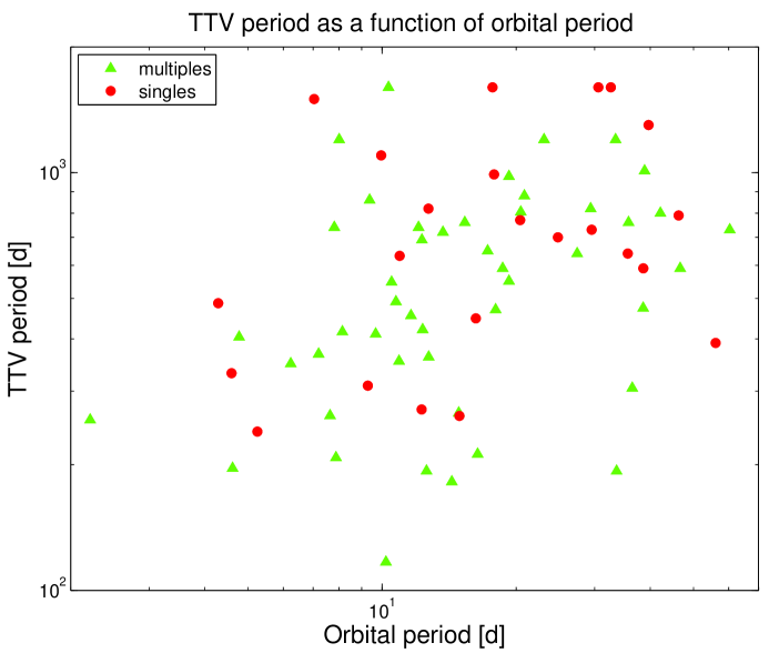
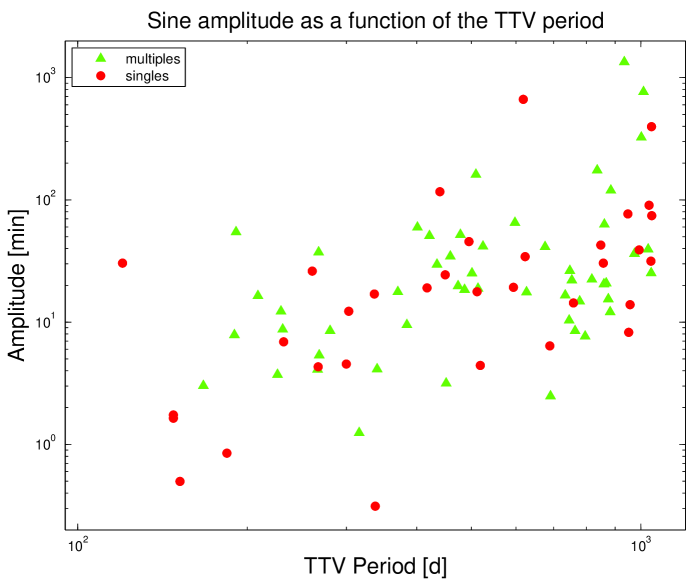
We have found an indication for some correlation, of $0.48$, between the KOI period and the period of its TTV, as can be seen in Figure 22. This is of no surprise, as the orbital period of a planet determines the natural time scale of the dynamical interaction, and therefore one can expect the TTV periodicity to be correlated with this time scale. Another correlation, of $0.51$, between the amplitudes and the periods of the detected TTV periodicities, emerged from our sample (see Figure 23), as was predicted, for example, by Agol et al. (2005). The same correlation appeared when we plotted the amplitude in units of the KOI orbital period.

Figure 22: The TTV period as a function of the orbital period. Red circles represent single KOIs, and green triangles represent multiples.

Figure 23: The amplitude of the TTV modulation as a function of its period. Red circles represent single KOIs, and green triangles represent multiples.

We point out a possible non-dynamical origin of some of the TTVs presented here. In particular, the short-period modulations could be due to either the long cadence sampling of Kepler or the stellar spot periodic activity (Sz13). We found evidence that five out of the $13$ short-period detected TTVs are due to the stellar periodicity. We also found that KOI-$13.01$ and $883.01$ show a periodicity induced by the Kepler sampling.

The sample of $143$ KOIs with significant TTVs includes $60$ systems discussed by F11 ($18$ KOIs), F12 ($38$ KOIs), Steffen et al. (2012a) ($8$ KOIs), and Steffen et al. (2013) ($15$ KOIs), all based only on a fraction of the data available now. References to those four works can be found in Table 4. It is interesting to compare the analysis of F11, F12 and Steffen et al. (2012b, 2013) on one hand and the present results on the other hand, and see how doubling the time span can change our assessment of the nature of the modulation. In many cases the time span of the first six quarters was not long enough to detect a local maximum and minimum of the TTV modulation, and therefore the periodicity of the modulation could not be estimated. One illustrious example is KOI-142, with its peak-to-peak amplitude of more than 1200 min (see Nesvorný et al., 2013).

One could hope that the accumulating details of the observed TTV could give some hints for the orbital elements of the perturbing unseen planet, at least for some of the single KOIs. However, as discussed already by Holman & Murray (2005) and Agol et al. (2005), the amplitude and periodicity of the TTV modulation depends on various parameters, in particular the mass and the orbital period of the unseen planet and how close the orbits of the two planets are to some mean motion resonance (e.g., Lithwick et al., 2012). Therefore, it is quite difficult to deduce the parameters of the unseen planet, although some stringent constraints can be derived, as was done by Ballard et al. (2011) and Nesvorný et al. (2012, 2013). We hope that the available catalog will motivate a similar work on other single-KOI systems with significant TTV.

One parameter that has interesting implications on our understanding of planetary formation is the relative inclination between the orbital plane of the observed planet and that of the presumed interacting planet for the cases of single KOIs with significant TTVs. Relative inclination can induce a precession of the orbital motion of the observed planet, which can manifest itself in a modulation of the transit duration and depth. Although the focus of the present work is on the TTVs, the catalog, which includes derived TDVs and TPVs, can, in principle, help to identify systems with a relative inclination. Furthermore, stringent upper limits on TDVs and TPVs for systems with detected TTVs can help to constrain the relative inclinations between the planets.

However, an observed precession is not necessarily induced by a planet with a non-vanishing relative inclination. An observed precession of the orbital plane just proves that the total angular momentum of the system is not parallel to the orbital angular momentum of the transiting planet. The origin of the precession could also be a misalignment of the stellar rotation axis relative to the angular momentum of the planet, an idea that was unthinkable not long ago, but has now a solid evidence in the accumulating data (see Winn, 2011). An example is KOI-13 (Szabó et al., 2011, see also Figure 1). Regardless, we suggest that systems with detected significant TDVs and TPVs deserve further close study.

Finally, we present here a systematic TTV analysis of twelve quarters of Kepler observations of all KOIs. One could expect that the derived TTVs, for the single KOIs in particular, could help in constructing a statistical picture of the frequency and architecture of the population of the planetary multiple systems of the Kepler KOIs (e.g., Ford et al., 2011, 2012b; Lissauer et al., 2011b; Steffen et al., 2010). To perform such a statistical analysis one needs to model the dependence of the detectability of TTV coherent modulation on the parameters of the unseen perturbing planet. The present catalog can be used for such a study.

References

- Agol et al. (2005) Agol, E., Steffen, J., Sari, R., & Clarkson, W. 2005, MNRAS, 359, 567
- Ballard et al. (2011) Ballard, S., Fabrycky, D., Fressin, F., et al. 2011, ApJ, 743, 200
- Batalha et al. (2012) Batalha, N. M., Rowe, J. F., Bryson, S. T., et al. 2012, arXiv:1202.5852
- Bonomo et al. (2012) Bonomo, A. S., Hébrard, G., Santerne, A., et al. 2012, A&A, 538, A96
- Borucki et al. (2011) Borucki, W. J., Koch, D. G., Basri, G., et al. 2011, ApJ, 736, 19
- Brown et al. (2011) Brown, T. M., Latham, D. W., Everett, M. E., & Esquerdo, G. A. 2011, AJ, 142, 112
- Carter et al. (2012) Carter, J. A., Agol, E., Chaplin, W. J., et al. 2012, Science, 337, 556
- Claret & Bloemen (2011) Claret, A., & Bloemen, S. 2011, A&A, 529, A75
- Cochran et al. (2011) Cochran, W. D., Fabrycky, D. C., Torres, G., et al. 2011, ApJS, 197, 7
- Desert et al. (2011) Desert, J.-M., Charbonneau, D., Demory, B.-O., et al. 2011, ApJS, 197, 14
- Fabrycky et al. (2012) Fabrycky, D. C., Ford, E. B., Steffen, J. H., et al. 2012, ApJ, 750, 114
- Ford et al. (2011) Ford, E. B., Rowe, J. F., Fabrycky, D. C., et al. 2011, ApJS, 197, 2
- Ford et al. (2012a) Ford, E. B., Fabrycky, D. C., Steffen, J. H., et al. 2012a, ApJ, 750, 113
- Ford et al. (2012b) Ford, E. B., Ragozzine, D., Rowe, J. F., et al. 2012b, ApJ, 756, 185
- Holman & Murray (2005) Holman, M. J., & Murray, N. W. 2005, Science, 307, 1288
- Holman et al. (2010) Holman, M. J., Fabrycky, D. C., Ragozzine, D., et al. 2010, Science, 330, 51
- Lagarais, Reeds & Wright (1998) Lagarais, J.C., J. A. Reeds, M. H. Wright, & P. E. Wright, ”Convergence Properties of the Nelder-Mead Simplex Method in Low Dimensions,” SIAM Journal of Optimization, Vol. 9 Number 1, pp. 112-147, 1998.
- Lissauer et al. (2011a) Lissauer, J. J., Fabrycky, D. C., Ford, E. B., et al. 2011a, Nature, 470, 53
- Lissauer et al. (2011b) Lissauer, J. J., Ragozzine, D., Fabrycky, D. C., et al. 2011b, ApJS, 197, 8
- Lithwick et al. (2012) Lithwick, Y., Xie, J., & Wu, Y. 2012, ApJ, 761, 122
- Mandel & Agol (2002) Mandel, K., & Agol, E. 2002, ApJ, 580, L171
- Mazeh et al. (2012) Mazeh, T., Nachmani, G., Sokol, G., Faigler, S., & Zucker, S. 2012, A&A, 541, A56
- McQuillan, Aigrain & Mazeh (2013) McQuillan, A., Aigrain, S., & Mazeh, T. 2013, MNRAS, 432, 1203
- Nesvorný et al. (2012) Nesvorný, D., Kipping, D. M., Buchhave, L. A., et al. 2012, Science, 336, 1133
- Nesvorný et al. (2013) Nesvorný, D., Kipping, D., Terrell, D., et al. 2013, arXiv:1304.4283
- Ofir & Dreizler (2012) Ofir, A., & Dreizler, S. 2012, arXiv:1206.5347
- Ragozzine & Kepler Team (2012) Ragozzine, D., & Kepler Team 2012, AAS/Division for Planetary Sciences Meeting Abstracts, 44, #200.04
- Sanchis-Ojeda et al. (2012) Sanchis-Ojeda, R., Fabrycky, D. C., Winn, J. N., et al. 2012, Nature, 487, 449
- Santerne et al. (2012) Santerne, A., Díaz, R. F., Moutou, C., et al. 2012, A&A, 545, A76
- Shporer et al. (2011) Shporer, A., Jenkins, J. M., Rowe, J. F., et al. 2011, AJ, 142, 195
- Steffen et al. (2010) Steffen, J. H., Batalha, N. M., Borucki, W. J., et al. 2010, ApJ, 725, 1226
- Steffen et al. (2011) Steffen, J. H., Quinn, S. N., Borucki, W. J., et al. 2011, MNRAS, 417, L31
- Steffen et al. (2012a) Steffen, J. H., Fabrycky, D. C., Ford, E. B., et al. 2012a, MNRAS, 421, 2342
- Steffen et al. (2012b) Steffen, J. H., Ford, E. B., Rowe, J. F., et al. 2012b, ApJ, 756, 186
- Steffen et al. (2013) Steffen, J. H., Fabrycky, D. C., Agol, E., et al. 2013, MNRAS, 428, 1077
- Szabó et al. (2011) Szabó, G. M., Szabó, R., Benkő, J. M., et al. 2011, ApJ, 736, L4
- Szabó et al. (2012) Szabó, G. M., Pál, A., Derekas, A., et al. 2012, MNRAS, 421, L122
- Szabó et al. (2013) Szabó, R., Szabó, G. M., Dálya, G., et al. 2013, A&A, 553, A17
- Tamuz, Mazeh & North (2006) Tamuz, O., Mazeh, T., & North, P. 2006, MNRAS, 367, 1521
- Tingley et al. (2011) Tingley, B., Palle, E., Parviainen, H., et al. 2011, A&A, 536, L9
- Wang et al. (2012) Wang, S., Ji, J., & Zhou, J.-L. 2012, ApJ, 753, 170
- Winn (2011) Winn, J. N. 2011, European Physical Journal Web of Conferences, 11, 5002
- Xie (2012) Xie, J.-W. 2012, arXiv:1208.3312