A Non-Perturbative Construction of the Fermionic Projector on Globally Hyperbolic Manifolds I – Space-Times of Finite Lifetime

Abstract.

We give a functional analytic construction of the fermionic projector on a globally hyperbolic Lorentzian manifold of finite lifetime. The integral kernel of the fermionic projector is represented by a two-point distribution on the manifold. By introducing an ultraviolet regularization, we get to the framework of causal fermion systems. The connection to the “negative-energy solutions” of the Dirac equation and to the WKB approximation is explained and quantified by a detailed analysis of closed Friedmann-Robertson-Walker universes.

1. Introduction

The fermionic projector was introduced in [8] as an operator which gives a splitting of the solution space of the Dirac equation into two subspaces (see also [9, Chapter 2] and [12]). In a static space-time, these subspaces reduce to the spaces of positive and negative energy which are familiar from the usual Dirac sea construction. The significance of the fermionic projector lies in the fact that it can be constructed canonically even in the time-dependent setting. It plays a central role in the fermionic projector approach to relativistic quantum field theory (see the review article [11] and the references therein).

So far, the fermionic projector was only constructed perturbatively in a formal power expansion in the potentials in the Dirac equation. In the present paper, we give a non-perturbative construction of the fermionic projector. To this end, we consider the Dirac equation on a globally hyperbolic Lorentzian manifold. For technical simplicity, we assume that space-time has finite lifetime. A space-time of infinite lifetime (like Minkowski space) can be treated with the same ideas and methods, using the so-called mass oscillation property as an additional technical tool. Since the mass oscillation property is of independent interest, we decided to work out the case of an infinite lifetime in a separate paper [17].

In order to explain the basic difficulty which prevented a non-perturbative treatment so far, we briefly outline the construction in [8] on a non-technical level. Suppose that we consider the Dirac equation in Minkowski space $(\mycal M,\langle.,.\rangle)$ in a given external potential ${\mathscr{B}}$,

$$(i\gamma^{j}\partial_{j}+{\mathscr{B}}-m)\psi=0\>.$$

Then the advanced and retarded Green’s functions $s^{\vee}_{m}$ and $s^{\wedge}_{m}$ are solutions of the distributional equations

$$(i\gamma^{j}\partial_{j}+{\mathscr{B}}-m)\,s^{\vee}_{m}(x,y)=\delta^{4}(x-y)=(i\gamma^{j}\partial_{j}+{\mathscr{B}}-m)\,s^{\wedge}_{m}(x,y)\>.$$

They are uniquely defined by the conditions that the distribution $s^{\vee}(x,.)$ (and $s^{\wedge}(x,.)$) should be supported in the causal future (respectively past) of $x$. Taking the difference of the advanced and retarded Green’s function gives a solution of the homogeneous Dirac equation, which we refer to as the causal fundamental solution $k_{m}$,

$$k_{m}(x,y):=\frac{1}{2\pi i}\left(s^{\vee}(x,y)-s^{\wedge}(x,y)\right).$$

We also consider $k_{m}$ as the integral kernel of a corresponding operator

$$(k_{m}(\psi))(x):=\int Mk_{m}(x,y)\>\psi(y)\>d^{4}y\>,$$

which acts on the wave functions in space-time. Here the integral merely is a notation to indicate a distribution acting on a test function (thus $k_{m}(\psi)=k_{m}(.,\psi)$ is the distribution obtained by evaluating the second argument of the bi-distribution $k_{m}(.,.)$ with $\psi$). Formally, the fermionic projector is obtained by taking the absolute value of this operator,

$$p_{m}\overset{\text{formally}}{:=}|k_{m}|\>,$$ (1.1)

and by forming the combination

$$P(x,y):=\frac{1}{2}\left(p_{m}(x,y)-k_{m}(x,y)\right)$$

(for the rescaling procedure needed to obtain the proper normalization see [12]). The basic difficulty is related to the fact that taking the absolute value of $k_{m}$ in a rigorous way requires spectral methods in Hilbert spaces. But the operator $k_{m}$ acts on the wave functions in space-time, which do not form a Hilbert space. More specifically, $k_{m}$ is symmetric with respect to the Lorentz invariant inner product on the wave functions

$$\mathopen{<}\psi|\phi\mathclose{>}=\int M\overline{\psi(x)}\phi(x)\>d^{4}x$$ (1.2)

(where $\overline{\psi}\equiv\psi^{\dagger}\gamma^{0}$ is the so-called adjoint spinor; we here restrict attention to square integrable wave functions). But as (1.2) is not positive definite, the corresponding function space merely is a Krein space. There is a spectral theorem in Krein spaces (see for example [6, 22]), but this theorem only applies to so-called definitizable operators. The operator $k_{m}$, however, is not known to be definitizable, making it impossible to apply spectral methods in indefinite inner product spaces. The methods in [8] give a mathematical meaning to the absolute value in (1.1) in a perturbation expansion, leading to the so-called causal perturbation theory. But a non-perturbative treatment seemed out of reach.

We now outline our method for bypassing the above difficulty, again for an external potential in flat space-time. One ingredient is to work instead of the space of wave functions with the solution space of the Dirac equation. This solution space has a natural Lorentz invariant scalar product

$$(\psi|\phi):=\int_{\mathbb{R}^{3}}(\overline{\psi}\gamma^{0}\phi)(t,\vec{x})\>d^{3}x\>,$$ (1.3)

giving rise to a Hilbert space $\mathscr{H}_{m}$. Our starting point is the observation (see [7, Proposition 2.2]) that the operator $k_{m}$ relates the scalar product (1.3) to the space-time inner product (1.2) by

$$(\psi\,|\,k_{m}\,\phi)=\mathopen{<}\psi|\phi\mathclose{>}$$ (1.4)

(valid if $\psi$ is a solution of the Dirac equation; see Proposition 3.1 below). On the other hand, we can express the bilinear form $\mathopen{<}.|.\mathclose{>}$ in terms of the scalar product using a signature operator $\mathscr{S}$,

$$\mathopen{<}\psi|\phi\mathclose{>}=(\psi|\mathscr{S}\phi)$$ (1.5)

(valid if $\psi$ and $\phi$ are solutions of the Dirac equation; see equation (3.4) below). The operator $\mathscr{S}$ will turn out to be a bounded symmetric operator on the Hilbert space $(\mathscr{H}_{m},(.|.))$. Comparing (1.4) with (1.5), we find that on solutions of the Dirac equation, the operator $k_{m}$ can be identified with the operator $\mathscr{S}$. This makes it possible to use spectral theory in Hilbert spaces to define the absolute value in (1.1).

In Section 3, we will make this construction mathematically precise in the setting of a globally hyperbolic space-time of finite lifetime. We point out that all our constructions are manifestly covariant. They do not depend on the choice of a foliation of the manifold. It makes no difference whether the Cauchy surfaces are compact or non-compact. We do not need to make any assumptions on the asymptotic behavior of the metric at infinity.

In Section 4, it is explained how the fermionic projector gives rise to examples of causal fermion systems as defined in [14, Section 1].

Our construction of the fermionic projector gives a splitting of the solution space of the Dirac equation into two subspaces. For the physical interpretation, it is important to understand how these subspaces relate to the usual concept of solutions of positive and negative energy. To this end, we analyze the fermionic projector in a closed Friedmann-Robertson-Walker universe. This has the advantage that the Dirac equation reduces to an ODE in time, which can be analyzed in detail. In particular, the concept of “solutions of negative energy” (which for clarity we mostly refer to as “solutions of negative frequency”) can be made precise by a specific WKB approximation as worked out in [16]. In Section 5, it is shown that our definition of the fermionic projector agrees with the concept of “all solutions of negative frequency,” provided that the metric is “nearly constant” on the Compton scale as quantified in Theorem 5.1 and Theorem 5.2. It is remarkable that, in contrast to a Grönwall estimate, our error estimates do not involve a time integral of the error term. This means that small local errors of the WKB approximation do not “add up” to give a big error after a long time. Moreover, our estimates also apply near the big bang and big crunch singularities. Keeping these facts in mind, our estimates show that for our physical universe, the fermionic projector coincides with very high precision with the usual concept of the Dirac sea being composed of all negative-frequency solutions of the Dirac equation. This gives a rigorous justification of the physical concepts behind the fermionic projector approach.

In Section 6, we analyze what happens if the metric changes substantially on the Compton scale. To this end, we consider a closed Friedmann-Robertson-Walker universe with a scale function $R(\tau)$ being piecewise constant. Then, at the times when $R$ is discontinuous, the frequencies of the solutions change. As a consequence, the concept of positive or negative frequency becomes meaningless. In this situation, our constructions still apply, giving a well-defined fermionic projector. This fermionic projector consists of a mixture of positive and negative frequencies. Moreover, as we explain in an explicit example where $\mathscr{S}=0$, the fermionic projector may depend sensitively on the detailed geometry of space-time.

2. Preliminaries

Let $(\mycal M,g)$ be a smooth, globally hyperbolic Lorentzian manifold of dimension $k\geq 2$. For the signature of the metric we use the convention $(+,-,\ldots,-)$. As proven in [3], $\mycal M$ admits a smooth foliation $(\mycal N_{t})_{t\in\mathbb{R}}$ by Cauchy hypersurfaces. Thus $\mycal M$ is topologically the product of $\mathbb{R}$ with a $k-1$-dimensional manifold. In the case $k=4$ of a four-dimensional space-time, this implies that $\mycal M$ is spin (for details see [2, 23]). For a general space-time dimension we need to impose that $\mycal M$ is spin. We let $S\mycal M$ be the spinor bundle on $\mycal M$ and denote the smooth sections of the spinor bundle by $C^{\infty}(\mycal M,S\mycal M)$. Similarly, $C^{\infty}_{0}(\mycal M,S\mycal M)$ denotes the smooth sections with compact support. The sections of the spinor bundle are also referred to as wave functions. The fibres $S_{x}\mycal M$ are endowed with an inner product of signature $(n,n)$ with $n=2^{[k/2]-1}$ (where $[\cdot]$ is the Gauß bracket; for details see again [2, 23]), which we denote by $\mathopen{\prec}.|.\mathclose{\succ}_{x}$. The Lorentzian metric induces a Levi-Civita connection and a spin connection, which we both denote by $\nabla$. Every vector of the tangent space acts on the corresponding spinor space by Clifford multiplication. Clifford multiplication is related to the Lorentzian metric via the anti-commutation relations. Denoting the mapping from the tangent space to the linear operators on the spinor space by $\gamma$, we thus have

$$\gamma\>:\>T_{x}\mycal M\rightarrow\text{\rm{L}}(S_{x}\mycal M)\qquad\text{with}\qquad\gamma(u)\,\gamma(v)+\gamma(v)\,\gamma(u)=2\,g(u,v)\,\mbox{\rm 1 1}_{S_{x}(\mycal M)}\>.$$

We also write Clifford multiplication in components with the Dirac matrices $\gamma^{j}$ and use the short notation with the Feynman dagger, $\gamma(u)\equiv u^{j}\gamma_{j}\equiv\not{u}$. The connections, inner products and Clifford multiplication satisfy Leibniz rules and compatibility conditions; we refer to [2, 23] for details. Combining the spin connection with Clifford multiplication gives the geometric Dirac operator ${\mathcal{D}}=i\gamma^{j}\nabla_{j}$. In order to include the situation when an external potential is present, we add a multiplication operator ${\mathscr{B}}(x)\in\text{\rm{L}}(S_{x}\mycal M)$, which we assume to be smooth and symmetric with respect to the spin scalar product,

$${\mathscr{B}}\in C^{\infty}(\mycal M,\text{\rm{L}}(S\mycal M))\qquad\text{with}\qquad\mathopen{\prec}{\mathscr{B}}\phi|\psi\mathclose{\succ}_{x}=\mathopen{\prec}\phi|{\mathscr{B}}\psi\mathclose{\succ}_{x}\quad\forall\phi,\psi\in S_{x}\mycal M\>.$$ (2.1)

We then introduce the Dirac operator by

$${\mathcal{D}}:=i\gamma^{j}\nabla_{j}+{\mathscr{B}}\>:\>C^{\infty}(\mycal M,S\mycal M)\rightarrow C^{\infty}(\mycal M,S\mycal M)\>.$$ (2.2)

For a given real parameter $m$ (the “rest mass”), the Dirac equation reads

$$({\mathcal{D}}-m)\,\psi_{m}=0\>.$$ (2.3)

For clarity, solutions of the Dirac equation always carry a subscript $m$. We point out that throughout this paper, the case $m=0$ of a massless field is allowed.

In the Cauchy problem, one seeks for a solution of the Dirac equation with initial data $\psi N$ prescribed on a given Cauchy surface $\mycal N$. Thus in the smooth setting,

$$({\mathscr{D}}-m)\,\psi_{m}=0\>,\qquad\psi|_{\mycal N}=\psi N\in C^{\infty}(\mycal N,S\mycal M)\>.$$ (2.4)

This Cauchy problem has a unique solution $\psi_{m}\in C^{\infty}(\mycal M,S\mycal M)$. This can be seen either by considering energy estimates for symmetric hyperbolic systems (see for example [21]) or alternatively by constructing the Green’s kernel (see for example [1]). These methods also show that the Dirac equation is causal, meaning that the solution of the Cauchy problem only depends on the initial data in the causal past or future. In particular, if $\psi N$ has compact support, the solution $\psi_{m}$ will also have compact support on any other Cauchy hypersurface. This leads us to consider solutions $\psi_{m}$ in the class $C^{\infty}_{\text{sc}}(\mycal M,S\mycal M)$ of smooth sections with spatially compact support. On solutions in this class, one introduces the scalar product $(.|.)N$ by

$$(\psi_{m}|\phi_{m})N=2\pi\int N\mathopen{\prec}\psi_{m}|\not{\nu}\phi_{m}\mathclose{\succ}_{x}\>d\mu N(x)\>,$$ (2.5)

where $\not{\nu}$ denotes Clifford multiplication by the future-directed normal $\nu$ (we always adopt the convention that the inner product $\mathopen{\prec}.|\not{\nu}.\mathclose{\succ}_{x}$ is positive definite). This scalar product does not depend on the choice of the Cauchy surface $\mycal N$. To see this, we let $\mycal N^{\prime}$ be another Cauchy surface and $\Omega$ the space-time region enclosed by $\mycal N$ and $\mycal N^{\prime}$. Using the symmetry property in (2.1) together with (2.2) and (2.3), we obtain

$$\begin{split}i\nabla_{j}\mathopen{\prec}\psi_{m}|\gamma^{j}\phi_{m}\mathclose{\succ}_{x}&=\mathopen{\prec}(-i\nabla_{j})\psi_{m}|\gamma^{j}\phi_{m}\mathclose{\succ}_{x}+\mathopen{\prec}\psi_{m}|(i\gamma^{j}\nabla_{j})\phi_{m}\mathclose{\succ}_{x}\\ &=-\mathopen{\prec}{\mathcal{D}}\psi_{m}|\phi_{m}\mathclose{\succ}_{x}+\mathopen{\prec}\psi_{m}|{\mathcal{D}}\phi_{m}\mathclose{\succ}_{x}=0\>,\end{split}$$ (2.6)

showing that the vector field $\mathopen{\prec}\psi_{m}|\gamma^{j}\phi_{m}\mathclose{\succ}_{x}$ is divergence-free (“current conservation”). Integrating over $\Omega$ and applying the Gauß divergence theorem, we find that $(\psi_{m}|\phi_{m})N=(\psi_{m}|\phi_{m})_{\mycal N^{\prime}}$. In view of the independence of the choice of the Cauchy surface, we simply denote the scalar product (2.5) by $(.|.)$. Forming the completion, we obtain the Hilbert space $(\mathscr{H}_{m},(.|.))$. It consists of all weak solutions of the Dirac equation (2.3) which are square integrable over any Cauchy surface.

The retarded and advanced Green’s operators $s_{m}^{\wedge}$ and $s_{m}^{\vee}$ are linear mappings (see for example [7, 1])

$$s_{m}^{\wedge},s_{m}^{\vee}\>:\>C^{\infty}_{0}(\mycal M,S\mycal M)\rightarrow C^{\infty}_{\text{sc}}(\mycal M,S\mycal M)\>.$$

They satisfy the defining equation of the Green’s operator

$$({\mathcal{D}}-m)\left(s_{m}^{\wedge,\vee}\phi\right)=\phi\>.$$ (2.7)

Moreover, they are uniquely determined by the condition that the support of $s_{m}^{\wedge}\phi$ (or $s_{m}^{\vee}\phi$) lies in the future (respectively the past) of $\operatorname{supp}\phi$. The causal fundamental solution $k_{m}$ is introduced by

$$k_{m}:=\frac{1}{2\pi i}\left(s_{m}^{\vee}-s_{m}^{\wedge}\right)\>:\>C^{\infty}_{0}(\mycal M,S\mycal M)\rightarrow C^{\infty}_{\text{sc}}(\mycal M,S\mycal M)\cap\mathscr{H}_{m}\>.$$ (2.8)

Note that it maps to solutions of the Dirac equation. Moreover, the distribution $k_{m}(x,y)$ can be used to construct an explicit solution of the Cauchy problem, as we recall in the next lemma. We only sketch the proof, because in Lemma 3.10 an independent proof will be given.

Lemma 2.1.

The solution of the Cauchy problem (2.4) has the representation

$$\psi_{m}(x)=2\pi\int Nk_{m}(x,y)\,\not{\nu}\,\psi N(y)\>d\mu N(y)\>,$$

where $k_{m}(x,y)$ is the integral kernel of the operator $k_{m}$, i.e.

$$(k_{m}\phi)(x)=\int Mk_{m}(x,y)\,\phi(y)\>d\mu M(y)$$ (2.9)

(here again the integrals are a notation for a distribution acting on a test function).

Sketch of the Proof..

For the proof that $k_{m}$ can be represented with an integral kernel (2.9) and for analytic details on $k_{m}(x,y)$ we refer to [1]. In order to prove (2.4), it suffices to consider a point $x$ in the future of $\mycal N$, in which case (2.4) simplifies in view of (2.8) to

$$\psi_{m}(x)=i\int Ns^{\wedge}_{m}(x,y)\,\not{\nu}(y)\,\psi N(y)\>d\mu N(y)\>.$$

This identity is derived as follows: We let $\eta\in C^{\infty}(\mycal M)$ be a function which is identically equal to one at $x$ and on $\mycal N$, but such that the function $\eta\psi_{m}$ has compact support (for example, in a foliation $(\mycal N_{t})_{t\in\mathbb{R}}$ one can take $\eta=\chi(t)$ with $\chi\in C^{\infty}_{0}(\mathbb{R})$). Then, using (2.7),

$$\psi_{m}(x)=(\eta\psi_{m})(x)\overset{(*)}{=}s^{\wedge}_{m}\big{(}({\mathscr{D}}-m)(\eta\psi_{m})\big{)}=s^{\wedge}_{m}\big{(}i\gamma^{j}(\partial_{j}\eta)\,\psi_{m})\big{)}\>,$$ (2.10)

where we used (2.7) and the fact that $\psi_{m}$ is a solution of the Dirac equation. In ($*$) we used the identity

$$\psi=s^{\wedge}\big{(}({\mathscr{D}}-m)\psi\big{)}\qquad\text{for~{}$\psi\in C^{\infty}_{0}(\mycal M,S\mycal M)$}\>,$$

which follows from the uniqueness of the solution of the Cauchy problem, noting that the function $\psi-s^{\wedge}(({\mathscr{D}}-m)\psi)$ satisfies the Dirac equation and vanishes in the past of the support of $\psi$. To conclude the proof, as the function $\eta$ in (2.10) we choose a sequence $\eta_{\ell}$ which converges in the distributional sense to the function which in the future and past of $\mycal N$ is equal to one and zero, respectively. ∎

3. Functional Analytic Construction of the Fermionic Projector

3.1. The Space-Time Inner Product as a Dual Pairing

On the wave functions, one can introduce the Lorentz invariant inner product

$$\mathopen{<}\psi|\phi\mathclose{>}:=\int M\mathopen{\prec}\psi|\phi\mathclose{\succ}_{x}\>d\mu M\>.$$ (3.1)

In order to ensure that the space-time integral is finite, we assume that one factor has compact support. In particular, we can regard $\mathopen{<}.|.\mathclose{>}$ as the dual pairing

$$\mathopen{<}.|.\mathclose{>}\>:\>\mathscr{H}_{m}\times C^{\infty}_{0}(\mycal M,S\mycal M)\rightarrow\mathbb{C}\>.$$

The next proposition shows that the causal fundamental solution is the signature operator of this dual pairing.

Proposition 3.1.

For any $\psi_{m}\in\mathscr{H}_{m}$ and $\phi\in C^{\infty}_{0}(\mycal M,S\mycal M)$,

$$(\psi_{m}\,|\,k_{m}\,\phi)=\mathopen{<}\psi_{m}|\phi\mathclose{>}\>.$$ (3.2)

Proof.

We first give the proof under the additional assumption that $\psi_{m}\in C^{\infty}_{\text{sc}}(\mycal M,S\mycal M)$. We choose Cauchy surfaces $\mycal N_{+}$ and $\mycal N_{-}$ lying in the future and past of $\operatorname{supp}\phi$, respectively. Let $\Omega$ be the space-time region between these two Cauchy surfaces, i.e. $\partial\Omega=\mycal N_{+}\cup\mycal N_{-}$. Then, according to (2.8),

$$(\psi_{m}\,|\,k_{m}\,\phi) =(\psi_{m}\,|\,k_{m}\,\phi)_{\mycal N_{+}}=\frac{i}{2\pi}\>(\psi_{m}\,|\,s_{m}^{\wedge}\,\phi)_{\mycal N_{+}}$$

$$=\frac{i}{2\pi}\Big{[}(\psi_{m}\,|\,s_{m}^{\wedge}\,\phi)_{\mycal N_{+}}-(\psi_{m}\,|\,s_{m}^{\wedge}\,\phi)_{\mycal N_{-}}\Big{]}$$

$$=i\int_{\Omega}\nabla_{j}\mathopen{\prec}\psi_{m}\,|\,\gamma^{j}s_{m}^{\wedge}\phi\mathclose{\succ}_{x}\>d\mu(x)\>,$$

where in the last line we applied the Gauß divergence theorem and used (2.5). Using that $\psi_{m}$ satisfies the Dirac equation, a calculation similar to (2.6) yields

$$(\psi_{m}\,|\,k_{m}\,\phi)=\int_{\Omega}\mathopen{\prec}\psi_{m}\,|\,({\mathcal{D}}-m)\,s_{m}^{\wedge}\phi\mathclose{\succ}_{x}\>d\mu(x)\overset{\eqref{Greendef}}{=}\int_{\Omega}\mathopen{\prec}\psi_{m}|\phi\mathclose{\succ}_{x}\>d\mu(x)\>.$$

As $\phi$ is supported in $\Omega$, we can extend the last integration to all of $\mycal M$, giving the result.

In order to extend the result to general $\psi_{m}\in\mathscr{H}_{m}$, we use the following approximation argument. Let $\psi_{m}^{(n)}\in\mathscr{H}_{m}\cap C^{\infty}_{\text{sc}}(\mycal M,S\mycal M)$ be a sequence which converges in $\mathscr{H}_{m}$ to $\psi_{m}$. Then obviously $(\psi^{(n)}_{m}\,|\,k_{m}\,\phi)\rightarrow(\psi_{m}\,|\,k_{m}\,\phi)$. In order to show that the right side of (3.2) also converges, it suffices to prove that $\psi_{m}^{(n)}$ converges in $L^{2}_{\text{loc}}(\mycal M,S\mycal M)$ to $\psi_{m}$. Thus let $K\subset\mycal M$ be a compact set contained in the domain of a chart $(x,U)$. Using Fubini’s theorem, we obtain for any $\psi\in\mathscr{H}_{m}\cap C^{\infty}_{\text{sc}}(\mycal M,S\mycal M)$ the estimate

$$\int_{K}\mathopen{\prec}\psi|\not{\nu}\psi\mathclose{\succ}d\mu M=\int dx^{0}\int\mathopen{\prec}\psi|\not{\nu}\psi\mathclose{\succ}\sqrt{|g|}\>d^{3}x\leq C(K)\,(\psi|\psi)\>.$$

Applying this estimate to the functions $\psi=\psi^{(n)}_{m}-\psi^{(n^{\prime})}_{m}$, we see that $\psi^{(n)}_{m}$ converges in $L^{2}(K,S\mycal M)$ to a function $\tilde{\psi}$. This implies that $\psi^{(n)}_{m}$ converges to $\tilde{\psi}$ pointwise almost everywhere (with respect to the measure $d\mu M$). Moreover, the convergence of $\psi^{(n)}_{m}$ in $\mathscr{H}_{m}$ to $\psi_{m}$ implies that the restriction of $\psi^{(n)}_{m}$ to any Cauchy surface $\mycal N$ converges to $\psi_{m}|N$ pointwise almost everywhere (with respect to the measure $d\mu N$). It follows that $\tilde{\psi}=\psi_{m}|_{K}$, concluding the proof. ∎

Corollary 3.2.

The operator $k_{m}$, (2.8), is symmetric with respect to the inner product (3.1).

Proof.

Using Proposition 3.1, we obtain for all $\phi,\psi\in C^{\infty}_{0}(\mycal M,S\mycal M)$,

$$\mathopen{<}k_{m}\phi\,|\,\psi\mathclose{>}=(k_{m}\phi\,|\,k_{m}\psi)=\mathopen{<}\phi\,|\,k_{m}\psi\mathclose{>}\>,$$

concluding the proof. ∎

3.2. Space-Times of Finite Lifetime

For the construction of the fermionic projector, we need to assume that space-time has the following property.

Definition 3.3.

A globally hyperbolic manifold $(\mycal M,g)$ is said to be m-finite if there is a constant $c>0$ such that for all $\phi_{m},\psi_{m}\in\mathscr{H}_{m}\cap C^{\infty}_{\text{sc}}(\mycal M,S\mycal M)$, the function $\mathopen{\prec}\phi_{m}|\psi_{m}\mathclose{\succ}_{x}$ is integrable on $\mycal M$ and

$$|\mathopen{<}\phi_{m}|\psi_{m}\mathclose{>}|\leq c\>\|\phi_{m}\|\>\|\psi_{m}\|$$ (3.3)

(where $\|.\|=(.|.)^{\frac{1}{2}}$ is the norm on $\mathscr{H}_{m}$).

Before going on, let us briefly discuss which manifolds are $m$-finite.

Definition 3.4.

A globally hyperbolic manifold $(\mycal M,g)$ has finite lifetime if it admits a foliation $(\mycal N_{t})_{t\in(t_{0},t_{1})}$ by Cauchy surfaces with a bounded time function $t$ such that the function $\langle\nu,\partial_{t}\rangle$ is bounded on $\mycal M$ (where $\nu$ denotes the future-directed normal on $\mycal N_{t}$ and $\langle\nu,\partial_{t}\rangle\equiv g(\nu,\partial_{t})$).

Proposition 3.5.

Every globally hyperbolic manifold of finite lifetime is $m$-finite.

Proof.

Let $\phi_{m},\psi_{m}\in C^{\infty}_{\text{sc}}(\mycal M,S\mycal M)$ be solutions of the Dirac equation (2.3). Applying Fubini’s theorem and decomposing the volume measure, we obtain

$$\mathopen{<}\phi_{m}|\psi_{m}\mathclose{>}=\int M\mathopen{\prec}\phi_{m}|\psi_{m}\mathclose{\succ}(x)\>d\mu M(x)\\ =\int_{t_{0}}^{t_{1}}\int_{\mycal N_{t}}\mathopen{\prec}\phi_{m}|\psi_{m}\mathclose{\succ}\,\langle\nu,\partial_{t}\rangle\,dt\,d\mu_{\mycal N_{t}}$$

and thus

$$\big{|}\mathopen{<}\phi_{m}|\psi_{m}\mathclose{>}\big{|}\leq\sup M\langle\nu,\partial_{t}\rangle\int_{t_{0}}^{t_{1}}dt\int_{\mycal N_{t}}|\mathopen{\prec}\phi_{m}|\psi_{m}\mathclose{\succ}|\,d\mu_{\mycal N_{t}}\>.$$

Estimating the spatial integral by

$$\int_{\mycal N_{t}}|\mathopen{\prec}\phi_{m}|\psi_{m}\mathclose{\succ}|\,d\mu_{\mycal N_{t}}\leq\int_{\mycal N_{t}}\sqrt{\mathopen{\prec}\phi_{m}|\not{\nu}\phi_{m}\mathclose{\succ}}\>\sqrt{\mathopen{\prec}\psi_{m}|\not{\nu}\psi_{m}\mathclose{\succ}}\>d\mu_{\mycal N_{t}}\leq\|\phi_{m}\|\>\|\psi_{m}\|\>,$$

we conclude that

$$\big{|}\mathopen{<}\phi_{m}|\psi_{m}\mathclose{>}\big{|}\leq(t_{1}-t_{0})\>\sup M\langle\nu,\partial_{t}\rangle\>\|\phi_{m}\|\>\|\psi_{m}\|\>.$$

A denseness argument gives the result. ∎

Proposition 3.6.

On a globally hyperbolic manifold of finite lifetime, there is a constant $C<\infty$ such that the arc length of every smooth timelike curve is at most $C$.

Proof.

Let $\gamma$ be a timelike geodesic. Possibly after extending it, we can parametrize it by the time function $t\in(t_{0},t_{1})$ of our foliation. Then the vector field $\dot{\gamma}-\partial_{t}$ is tangential to $\mycal N_{t}$. Hence we can estimate the length of the geodesic by

$$L(\gamma)=\int_{t_{0}}^{t_{1}}\sqrt{\langle\dot{\gamma},\dot{\gamma}\rangle}\,dt\leq\int_{t_{0}}^{t_{1}}\sqrt{\langle\dot{\gamma},\nu\rangle\langle\nu,\dot{\gamma}\rangle}\,dt=\int_{t_{0}}^{t_{1}}\langle\nu,\partial_{t}\rangle\,dt\leq(t_{1}-t_{0})\sup M\langle\nu,\partial_{t}\rangle\>.$$

This concludes the proof. ∎

We do not know whether an upper bound on the length of timelike geodesics already implies that the space-time has finite lifetime in the sense of Definition 3.4. Moreover, we do not expect that every $m$-finite manifold has finite lifetime. Unfortunately, entering the study of these questions goes beyond the scope of the present paper.

3.3. The Fermionic Signature Operator and the Fermionic Projector

Let us assume that $(\mycal M,g)$ is $m$-finite. Then the space-time inner product can be extended by continuity to a bilinear form

$$\mathopen{<}.|.\mathclose{>}\>:\>\mathscr{H}_{m}\times\mathscr{H}_{m}\rightarrow\mathbb{C}\>.$$

Moreover, applying the Riesz representation theorem, we can uniquely represent this inner product with a signature operator $\mathscr{S}$,

$$\mathscr{S}\>:\>\mathscr{H}_{m}\rightarrow\mathscr{H}_{m}\qquad\text{with}\qquad\mathopen{<}\phi_{m}|\psi_{m}\mathclose{>}=(\phi_{m}\,|\,\mathscr{S}\,\psi_{m})\>.$$ (3.4)

We refer to $\mathscr{S}$ as the fermionic signature operator. It is obviously a symmetric operator. Moreover, it is bounded according to (3.3). We conclude that it is self-adjoint. The spectral theorem gives the spectral decomposition

$$\mathscr{S}=\int_{\sigma(\mathscr{S})}\lambda\>dE_{\lambda}\>,$$

where $E_{\lambda}$ is the spectral measure (see for example [26]). The spectral measure gives rise to the spectral calculus

$$f(\mathscr{S})=\int_{\sigma(\mathscr{S})}f(\lambda)\>dE_{\lambda}\>:\>\mathscr{H}_{m}\rightarrow\mathscr{H}_{m}\>,$$

where $f$ is a bounded Borel function on $\sigma(\mathscr{S})\subset\mathbb{R}$.

The spectral calculus for the fermionic signature operator is very useful because it gives rise to a corresponding spectral calculus for the operator $k_{m}$, as we now explain. Multiplying $k_{m}$ from the left by $f(\mathscr{S})$ with a bounded Borel function $f$ gives an operator

$$f(\mathscr{S})\,k_{m}\>:\>C^{\infty}_{0}(\mycal M,S\mycal M)\rightarrow\mathscr{H}_{m}\>.$$

This operator is again symmetric with respect to $\mathopen{<}.|.\mathclose{>}$, because for any $\phi,\psi\in C^{\infty}_{0}(\mycal M,S\mycal M)$,

$$\begin{split}\mathopen{<}f(\mathscr{S})\,k_{m}\,\phi\,|\,\psi\mathclose{>}&=(f(\mathscr{S})\,k_{m}\phi\,|\,k_{m}\psi)\\ &=(k_{m}\phi\,|\,f(\mathscr{S})\,k_{m}\psi)=\mathopen{<}\phi\,|\,f(\mathscr{S})\,k_{m}\,\psi\mathclose{>}\>,\end{split}$$ (3.5)

where in the first and last equality we applied Proposition 3.1. In order to make sense of products of such operators, we can consider the inner product $\mathopen{<}f(\mathscr{S})k_{m}\phi|g(\mathscr{S})k_{m}\psi\mathclose{>}$ (where $f,g$ are bounded Borel functions). Combining (3.4) with the spectral calculus for $\mathscr{S}$ and Proposition 3.1, we obtain

$$\begin{split}\mathopen{<}f(\mathscr{S})\,k_{m}\,\phi\,|\,g(\mathscr{S})\,k_{m}\,\psi\mathclose{>}&=(f(\mathscr{S})\,k_{m}\,\phi\,|\,\mathscr{S}\,g(\mathscr{S})\,k_{m}\,\psi)\\ &=(k_{m}\,\phi\,|\,(fg)(\mathscr{S})\>\mathscr{S}\,k_{m}\,\psi)=\mathopen{<}\phi\,|\,(fg)(\mathscr{S})\>\mathscr{S}\,k_{m}\,\psi\mathclose{>}\>.\end{split}$$ (3.6)

In view of (3.5), this identity can be written in the suggestive form

$$\left(f(\mathscr{S})k_{m}\right)\left(g(\mathscr{S})k_{m}\right)\overset{\text{formally}}{=}(fg)(\mathscr{S})\>\mathscr{S}\>k_{m}\>.$$ (3.7)

Note that this last equation makes no direct mathematical sense because the image of the operator $g(\mathscr{S})k_{m}$ does not lie in the domain of $k_{m}$, making it impossible to take the product. However, with (3.5) and (3.6) we have given this product a precise mathematical meaning.

We now use this procedure to construct the fermionic projector.

Definition 3.7.

Assume that the globally hyperbolic manifold $(\mycal M,g)$ is $m$-finite (see Definition 3.3). Then the operators $P_{\pm}\>:\>C^{\infty}_{0}(\mycal M,S\mycal M)\rightarrow\mathscr{H}_{m}$ are defined by

$$P_{+}=\chi_{[0,\infty)}(\mathscr{S})\,k_{m}\qquad\text{and}\qquad P_{-}=-\chi_{(-\infty,0)}(\mathscr{S})\,k_{m}$$ (3.8)

(where $\chi$ denotes the characteristic function). The fermionic projector $P$ is defined by $P=P_{-}$.

Proposition 3.8.

For all $\phi,\psi\in C^{\infty}_{0}(\mycal M,S\mycal M)$, the operators $P_{\pm}$ have the following properties:

$$\mathopen{<}P_{\pm}\,\phi\,|\,\psi\mathclose{>} =\mathopen{<}\phi\,|\,P_{\pm}\,\psi\mathclose{>}$$ (symmetry) (3.9)

$$\mathopen{<}P_{+}\,\phi\,|\,P_{-}\,\psi\mathclose{>} =0$$ (orthogonality) (3.10)

$$\mathopen{<}P_{\pm}\,\phi\,|\,P_{\pm}\,\psi\mathclose{>} =\mathopen{<}\phi\,|\,|\mathscr{S}|P_{\pm}\,\psi\mathclose{>} \text{(normalization)}\>.$$ (3.11)

Moreover, the image of $P_{\pm}$ is the positive respectively negative spectral subspace of $\mathscr{S}$, meaning that

$$\overline{P_{+}(C^{\infty}_{0}(\mycal M,S\mycal M))}=E_{(0,\infty)}(\mathscr{H}_{m})\>,\qquad\overline{P_{-}(C^{\infty}_{0}(\mycal M,S\mycal M))}=E_{(-\infty,0)}(\mathscr{H}_{m})\>.$$

Proof.

This follows immediately from (3.5), (3.6) and the functional calculus for self-adjoint operators in Hilbert spaces. ∎

We finally explain the normalization property (3.11). We first point out that, due to the factor $|\mathscr{S}|$ on the right of (3.11), the fermionic projector is not idempotent and is thus not a projection operator. The projection property could have been arranged by modifying (3.8) to

$$P=-\chi_{(-\infty,0)}(\mathscr{S})\,|\mathscr{S}|^{-1}\,k_{m}\>.$$

However, we prefer the definition (3.8) and the normalization (3.11). This normalization can be understood by working with a spatial normalization integral, as we now explain. In view of Lemma 2.1, we can introduce an operator $\Pi$ by

$$\Pi\>:\>\mathscr{H}_{m}\rightarrow\mathscr{H}_{m}\>,\qquad(\Pi\,\psi_{m})(x)=-2\pi\int NP(x,y)\,\not{\nu}\,(\psi_{m})|N(y)\>d\mu N(y)\>,$$ (3.12)

where $\mycal N$ is any Cauchy surface.

Proposition 3.9.

The operator $\Pi$ is a projection operator on $\mathscr{H}_{m}$.

Proof.

Combining Lemma 2.1 with (3.8), we find that $\Pi$ coincides with the operator $\chi_{(-\infty,0)}(\mathscr{S})$, which is obviously a projection operator. ∎

Since (3.12) involves a spatial integral, we also refer to $P$ as the fermionic projector with spatial normalization. We remark that an alternative method for normalizing the fermionic projector is to work with a $\delta$-normalization in the mass parameter (for details see [8, eqns (3.19)-(3.21)] or [12]). However, this so-called mass normalization can only be used in space-times of infinite lifetime. A detailed comparison of the spatial normalization and the mass normalization is given in [18].

3.4. Explicit Formulas in a Foliation

It is instructive to supplement the previous abstract constructions by explicit formulas in a foliation. We always work with the following particularly convenient class of foliations. As shown in [4, 24], there are foliations $(\mycal N_{t})_{t\in\mathbb{R}}$ by Cauchy surfaces where the gradient of the time function is orthogonal to the leaves and the lapse function is bounded, i.e.

$$g=\beta^{2}\,dt^{2}-g_{\mycal N_{t}}\qquad\text{with}\qquad 0<\beta\leq 1\>,$$ (3.13)

where $g_{\mycal N_{t}}$ is the induced Riemannian metric on $\mycal N_{t}$, and the lapse function $\beta$ is a smooth function on $\mycal M$. We remark that in space-times of finite life time (see Definition 3.4), the time parameter $t$ could be chosen on a bounded interval. In this case, for convenience we prefer to parametrize $t$ on all of $\mathbb{R}$, such that $\lim\limits_{t\rightarrow\pm\infty}\beta=0$. We denote space-time points by $(t,x)$ with $t\in\mathbb{R}$ and $x\in\mycal N_{t}$. Moreover, we denote the scalar product (2.5) for $\mycal N=\mycal N_{t}$ by $(.|.)_{t}$, and the corresponding Hilbert space by $(\mathscr{H}_{t},(.|.)_{t})$. Solving the Cauchy problem with initial data on $\mycal N_{t}$ and evaluating the solution at another time $t^{\prime}$ gives rise to a unitary time evolution operator

$$U^{t^{\prime},t}\>:\>\mathscr{H}_{t}\rightarrow\mathscr{H}_{t^{\prime}}\>.$$

Clearly, the unitary time evolution operators are a representation of the group $(\mathbb{R},+)$. The time evolution also gives rise to the unitary mapping

$$\iota_{m}\>:\>\mathscr{H}_{t}\rightarrow\mathscr{H}_{m}\>,\quad(\iota_{m}\psi)(t^{\prime},x)=(U^{t^{\prime},t}\,\psi)(x)\>,$$

which allows us to canonically identify each Hilbert space $(\mathscr{H}_{t},(.|.)_{t})$ with $(\mathscr{H}_{m},(.|.))$. We denote the restriction of a smooth Dirac wave function $\psi\in C^{\infty}(\mycal M,S\mycal M)$ to the hypersurface $\mycal N_{t}$ by $\psi_{|t}$.

Lemma 3.10.

For every $\phi\in C^{\infty}_{0}(\mycal M,S\mycal M)$,

$$(s^{\wedge}_{m}\phi)(t,x) =-i\int_{-\infty}^{t}\Big{(}U^{t,t^{\prime}}\!\big{(}\beta\not{\nu}\phi_{|t^{\prime}}\big{)}\Big{)}(x)\>dt^{\prime}$$ (3.14)

$$(k_{m}\phi)(t,x) =\frac{1}{2\pi}\int_{-\infty}^{\infty}\Big{(}U^{t,t^{\prime}}\!\big{(}\beta\not{\nu}\phi_{|t^{\prime}}\big{)}\Big{)}(x)\>dt^{\prime}\>.$$ (3.15)

Proof.

The Dirac operator can be written as

$${\mathcal{D}}=\beta^{-1}\not{\nu}\left(i\partial_{t}-H_{t}\right)\>,$$

where $H_{t}$ is a purely spatial operator acting on $\mathscr{H}_{t}$ (the “Hamiltonian”). We apply the Dirac operator to the right side of (3.14), which we denote by $F(t,x)$. As the integrand in (3.14) is a solution of the Dirac equation, only the derivative of the limit of integration needs to be taken into account,

$$({\mathcal{D}}-m)F(t,x)=\big{(}\beta^{-1}\not{\nu}(t,x)\big{)}\big{(}U^{t,t}(\beta\not{\nu}\phi_{|t})\big{)}(x)\>.$$

Using that $U^{t,t}$ is the identity, we conclude that

$$({\mathcal{D}}-m)F(t,x)=\phi(t,x)\>.$$

Hence $F(t,x)$ satisfies the defining equation of the Green’s operator (2.7). Moreover, it is obvious that $F(t,x)$ vanishes if $t$ is in the past of the support of $\phi$. The unique solution of the Cauchy problem gives the result.

Repeating the above argument for the advanced Green’s operator gives

$$(s^{\vee}_{m}\phi)(t,x)=i\int_{t}^{\infty}\Big{(}U^{t,t^{\prime}}\!\big{(}\beta\not{\nu}\phi_{|t^{\prime}}\big{)}\Big{)}(x)\>dt^{\prime}\>.$$

We finally apply (2.8) to obtain (3.15). ∎

For what follows, it is useful to identify $\mathscr{H}_{m}$ with the Hilbert space $\mathscr{H}_{t_{0}}$ for some fixed time $t_{0}$. The formulas of the previous lemma are then rewritten by multiplying with the time evolution operator. For example,

$$k_{m}\phi=\frac{1}{2\pi}\int_{-\infty}^{\infty}U^{t_{0},t}\big{(}\beta\not{\nu}\,\phi\big{)}_{|t}\>dt\>:\>C^{\infty}_{0}(\mycal M,S\mycal M)\rightarrow\mathscr{H}_{t_{0}}\>.$$ (3.16)

Lemma 3.11.

Assume that $(\mycal M,g)$ is $m$-finite. Then the fermionic signature operator $\mathscr{S}$ as defined by (3.4) has the representation

$$\mathscr{S}=\frac{1}{2\pi}\int_{-\infty}^{\infty}U^{t_{0},t}\,(\beta\not{\nu})_{|t}\,U^{t,t_{0}}\>dt\;:\;\mathscr{H}_{t_{0}}\rightarrow\mathscr{H}_{t_{0}}\>.$$

Proof.

Rewriting the space-time integral in (3.1) with Fubini’s theorem and using the identity $\not{\nu}^{2}=\mbox{\rm 1 1}$, we obtain

$$\mathopen{<}\phi_{m}|\psi_{m}\mathclose{>} =\int_{-\infty}^{\infty}\bigg{(}\int_{\mycal N_{t}}\mathopen{\prec}\phi_{m}|\psi_{m}\mathclose{\succ}_{(t,x)}\>\beta(t,x)\>d\mu_{\mycal N_{t}}(x)\bigg{)}\>dt$$

$$=\frac{1}{2\pi}\int_{-\infty}^{\infty}(\phi_{m}\,|\,(\beta\not{\nu})_{|t}\,\psi_{m})_{t}\>dt$$

$$=\frac{1}{2\pi}\int_{-\infty}^{\infty}(\phi_{|t_{0}}\,|\,U^{t_{0},t}\,(\beta\not{\nu})_{|t}\,U^{t,t_{0}}\,\psi_{|t_{0}})_{t_{0}}\>dt\>.$$

Comparing with (3.4) gives the result. ∎

Iterating (3.15), we can make the following formal calculation,

$$(k_{m}\,k_{m}\,\phi)_{|t_{0}} =\frac{1}{4\pi^{2}}\int_{-\infty}^{\infty}dt\int_{-\infty}^{\infty}dt^{\prime}\>U^{t_{0},t}\big{(}\beta\not{\nu}\big{)}_{|t}U^{t,t^{\prime}}\!\big{(}\beta\not{\nu}\phi\big{)}_{|t^{\prime}}$$

$$=\frac{1}{4\pi^{2}}\int_{-\infty}^{\infty}dt\int_{-\infty}^{\infty}dt^{\prime}\>U^{t_{0},t}(\beta\not{\nu})_{|t}\,U^{t,t_{0}}\;U^{t_{0},t^{\prime}}(\beta\not{\nu}\phi)_{|t^{\prime}}\>,$$

where in the second line we used the group property of the time evolution operator. Comparing with (3.16), we obtain the simple relation

$$k_{m}\,k_{m}\overset{\text{formally}}{=}\mathscr{S}\,k_{m}\>.$$

This is precisely the relation (3.7) in the special case $f,g\equiv 1$. Iteration gives similar formal expressions for polynomials of $k_{m}$, from which (3.7) can be obtained formally by approximation. Although the last arguments are only formal, they explain how the functional calculus (3.7) comes about. In order to give this functional calculus a mathematical meaning, one needs to evaluate weakly as is made precise by (3.5) and (3.6).

3.5. Representation as a Distribution

We now represent the fermionic projector by a two-point distribution on $\mycal M$.

Theorem 3.12.

There is a unique distribution ${\mathcal{P}}\in{\mathscr{D}}^{\prime}(\mycal M\times\mycal M)$ such that for all $\phi,\psi\in C^{\infty}_{0}(\mycal M,S\mycal M)$,

$$\mathopen{<}\phi|P\psi\mathclose{>}={\mathcal{P}}\big{(}\overline{\phi}\otimes\psi\big{)}\>.$$

Proof.

According to Proposition 3.1 and Definition 3.7,

$$\mathopen{<}\phi|P\psi\mathclose{>}=(k_{m}\phi\,|\,P\psi)=-(k_{m}\phi\,|\,\chi_{(-\infty,0)}(\mathscr{S})\,k_{m}\psi)\>.$$

Since the norm of the operator $\chi_{(-\infty,0)}(\mathscr{S})$ is bounded by one, we conclude that

$$|\mathopen{<}\phi|P\psi\mathclose{>}|\leq\|k_{m}\phi\|\>\|k_{m}\psi\|=(\mathopen{<}\phi|k_{m}\phi\mathclose{>}\>\mathopen{<}\psi|k_{m}\psi\mathclose{>})^{\frac{1}{2}}\>,$$

where in the last step we again applied Proposition 3.1. As $k_{m}\in{\mathscr{D}}^{\prime}(\mycal M\times\mycal M)$, the right side is continuous on ${\mathscr{D}}(\mycal M\times\mycal M)$. We conclude that also $\mathopen{<}\phi|P\psi\mathclose{>}$ is continuous on ${\mathscr{D}}(\mycal M\times\mycal M)$. The result now follows from the Schwartz kernel theorem (see [20, Theorem 5.2.1], keeping in mind that this theorem applies just as well to bundle-valued distributions on a manifold simply by working with the components in local coordinates and a local trivialization). ∎

In order to get the connection to [9], it is convenient to use the standard notation with an integral kernel $P(x,y)$,

$$\mathopen{<}\phi|P\psi\mathclose{>} =\iint_{\mycal M\times\mycal M}\mathopen{\prec}\phi(x)\,|\,P(x,y)\,\psi(y)\mathclose{\succ}_{x}\>d\mu M(x)\>d\mu M(y)$$

$$(P\psi)(x) =\int_{\mycal M}P(x,y)\,\psi(y)\>d\mu M(y)$$

(where $P(.,.)$ coincides with the distribution ${\mathcal{P}}$ above). In view of Proposition 3.8, we know that last integral is not only a distribution, but a function which is square integrable over every Cauchy surface. Moreover, the symmetry of $P$, (3.9), implies that

$$P(x,y)^{*}=P(y,x)\>,$$

where the star denotes the adjoint with respect to the spin scalar product. Finally, the spatial normalization property of Proposition 3.9 makes it possible to obtain the following representation of the fermionic projector.

Proposition 3.13.

Let $(\psi_{j})_{j\in\mathbb{N}}$ be an orthonormal basis of the subspace $\chi_{(-\infty,0)}(\mathscr{S})$ of the Hilbert space $\mathscr{H}_{m}$. Then

$$P(x,y)=-\sum_{j=1}^{\infty}|\psi_{j}(x)\mathclose{\succ}\mathopen{\prec}\psi_{j}(y)|$$ (3.17)

with convergence in ${\mathscr{D}}^{\prime}(\mycal M\times\mycal M)$.

Proof.

Being a projector on $\chi_{(-\infty,0)}(\mathscr{S})$, the operator $\Pi$ defined by (3.12) has the representation $\Pi=\sum_{j}|\psi_{j})(\psi_{j}|$ and thus, in view of (2.5),

$$(\Pi\phi_{m})(x)=2\pi\sum_{j\in\mathbb{N}}\psi_{j}(x)\int N\mathopen{\prec}\psi_{j}(y)|\not{\nu}\phi_{m}(y)\mathclose{\succ}_{y}\>d\mu N(y)\>.$$

Comparing with (3.12) and using that $\phi_{m}$ can be chosen arbitrarily on $\mycal N$, one sees that (3.17) holds for all $y\in\mycal N$. Since the Cauchy surface $\mycal N$ can be chosen to intersect any given space-time point, the result follows. ∎

4. Connection to the Framework of Causal Fermion Systems

We now explain the relation to the framework of causal fermion systems as introduced in [14] (see also [13]). In order to get into this framework, we need to introduce an ultraviolet regularization. This is done most conveniently with so-called regularization operators.

Definition 4.1.

A family $({\mathfrak{R}}_{\varepsilon})_{\varepsilon>0}$ of bounded linear operators on $\mathscr{H}_{m}$ are called regularization operators if they have the following properties:

• Solutions of the Dirac equation are mapped to continuous solutions,

  $${\mathfrak{R}}_{\varepsilon}\>:\>\mathscr{H}_{m}\rightarrow C^{0}(\mycal M,S\mycal M)\cap\mathscr{H}_{m}$$

• For every $\varepsilon>0$ and $x\in\mycal M$, there is a constant $c>0$ such that

  $$\|({\mathfrak{R}}_{\varepsilon}\psi_{m})(x)\|\leq c\,\|\psi_{m}\|\qquad\forall\;\psi_{m}\in\mathscr{H}_{m}\>.$$ (4.1)

  (where the norm on the left is any norm on $S_{x}\mycal M$).

• In the limit $\varepsilon\searrow 0$, the regularization operators go over to the identity with strong convergence of ${\mathfrak{R}}_{\varepsilon}$ and ${\mathfrak{R}}_{\varepsilon}^{*}$, i.e.

  $${\mathfrak{R}}_{\varepsilon}\psi_{m},\;{\mathfrak{R}}_{\varepsilon}^{*}\psi_{m}\xrightarrow{\varepsilon\searrow 0}\psi_{m}{\text{ in~{}$\mathscr{H}_{m}$}}\qquad\forall\;\psi_{m}\in\mathscr{H}_{m}\>.$$ (4.2)

There are many possibilities to choose regularization operators. As a typical example, one can choose finite-dimensional subspaces $\mathscr{H}^{(\ell)}\subset C^{\infty}_{\text{sc}}(\mycal M,S\mycal M)\cap\mathscr{H}_{m}$ which are an exhaustion of $\mathscr{H}_{m}$ in the sense that $\mathscr{H}^{(0)}\subset\mathscr{H}^{(1)}\subset\cdots$ and $\mathscr{H}_{m}=\overline{\cup_{\ell}\mathscr{H}^{(\ell)}}$. Setting $\ell(\varepsilon)=\max([0,1/\varepsilon]\cap\mathbb{N})$, we can introduce the operators ${\mathfrak{R}}_{\varepsilon}$ as the orthogonal projection operators to $\mathscr{H}^{(\ell(\varepsilon))}$. An alternative method is to choose a Cauchy hypersurface $\mycal N$, to mollify the restriction $\psi_{m}|N$ to the Cauchy surface on the length scale $\varepsilon$, and to define ${\mathfrak{R}}_{\varepsilon}\psi_{m}$ as the solution of the Cauchy problem for the mollified initial data.

Given regularization operators ${\mathfrak{R}}_{\varepsilon}$, for any $\varepsilon>0$ we introduce the particle space $(\mathscr{H}_{\text{\tiny{particle}}},\langle.|.\rangle_{\mathscr{H}_{\text{\tiny{particle}}}})$ as the Hilbert space

$$\mathscr{H}_{\text{\tiny{particle}}}=\ker\big{(}\mathfrak{R}_{\varepsilon}\,\chi_{(-\infty,0)}(\mathscr{S})\big{)}^{\perp}\>,\qquad\langle.|.\rangle_{\mathscr{H}_{\text{\tiny{particle}}}}=(.|.)|_{\mathscr{H}_{\text{\tiny{particle}}}\times\mathscr{H}_{\text{\tiny{particle}}}}\>.$$

Next, for any $x\in\mycal M$ we consider the bilinear form

$$b\>:\>\mathscr{H}_{\text{\tiny{particle}}}\times\mathscr{H}_{\text{\tiny{particle}}}\rightarrow\mathbb{C}\>,\quad b(\psi_{m},\phi_{m})=-\mathopen{\prec}({\mathfrak{R}}_{\varepsilon}\,\psi_{m})(x)\>|\>({\mathfrak{R}}_{\varepsilon}\,\phi_{m})(x)\mathclose{\succ}_{x}\>.$$

This bilinear form is bounded in view of (4.1). The local correlation operator $F^{\varepsilon}(x)$ is defined as the signature operator of this bilinear form, i.e.

$$b(\psi_{m},\phi_{m})=\langle\psi_{m}\,|\,F^{\varepsilon}(x)\,\phi_{m}\rangle_{\mathscr{H}_{\text{\tiny{particle}}}}\qquad\text{for all~{}$\psi_{m},\phi_{m}\in\mathscr{H}_{\text{\tiny{particle}}}$}\>.$$

Taking into account that the spin scalar product has signature $(n,n)$, the local correlation operator is a symmetric operator in $\text{\rm{L}}(\mathscr{H}_{\text{\tiny{particle}}})$ of rank at most $2n$, which has at most $n$ positive and at most $n$ negative eigenvalues. Finally, we introduce the universal measure $d\rho=F^{\varepsilon}_{*}\,d\mu M$ as the push-forward of the volume measure on $\mycal M$ under the mapping $F^{\varepsilon}$ (thus $\rho(\Omega):=\mu M((F^{\varepsilon})^{-1}(\Omega))$). Omitting the subscript “particle”, we thus obtain a causal fermion system as defined in [14, Section 1.2]:

Definition 4.2.

Given a complex Hilbert space $(\mathscr{H},\langle.|.\rangle_{\mathscr{H}})$ (the “particle space”) and a parameter $n\in\mathbb{N}$ (the “spin dimension”), we let ${\mathscr{F}}\subset\text{\rm{L}}(\mathscr{H})$ be the set of all self-adjoint operators on $\mathscr{H}$ of finite rank, which (counting with multiplicities) have at most $n$ positive and at most $n$ negative eigenvalues. On ${\mathscr{F}}$ we are given a positive measure $\rho$ (defined on a $\sigma$-algebra of subsets of ${\mathscr{F}}$), the so-called universal measure. We refer to $(\mathscr{H},{\mathscr{F}},\rho)$ as a causal fermion system.

The formulation as a causal fermion system gives contact to a general mathematical framework in which there are many inherent analytic and geometric structures (see [10, 13]). In particular, the differential geometric objects of spin geometry have a canonical generalization to the regularized theory. Namely, starting from a causal fermion system $(\mathscr{H},{\mathscr{F}},\rho)$ one defines space-time $M$ as the support of the universal measure, $M:=\operatorname{supp}\rho$. Note that with this definition, the space-time points $x,y\in M$ are operators on $\mathscr{H}$ (thinking of our above construction of the causal fermion system, this means that we identify a space-time point $x$ with its local correlation operator $F^{\varepsilon}(x)$). On $M$, we consider the topology induced by ${\mathscr{F}}\subset\text{\rm{L}}(\mathscr{H})$. The causal structure is encoded in the spectrum of the operator products $xy$:

Definition 4.3.

For any $x,y\in{\mathscr{F}}$, the product $xy$ is an operator of rank at most $2n$. We denote its non-trivial eigenvalues by $\lambda^{xy}_{1},\ldots,\lambda^{xy}_{2n}$ (where we count with algebraic multiplicities). The points $x$ and $y$ are called timelike separated if the $\lambda^{xy}_{j}$ are all real and not all equal. They are said to be spacelike separated if all the $\lambda^{xy}_{j}$ have the same absolute value. In all other cases, the points $x$ and $y$ are said to be lightlike separated.

Next, we define the spin space $S_{x}$ by $S_{x}=x(\mathscr{H})\subset\mathscr{H}$ endowed with the inner product $\mathopen{\prec}.|.\mathclose{\succ}_{x}:=-\langle.|x.\rangle_{\mathscr{H}}$. The kernel of the fermionic projector with regularization is introduced by

$$P^{\varepsilon}(x,y)=\pi_{x}\,y\>:\>S_{y}\rightarrow S_{x}\>,$$ (4.3)

where $\pi_{x}$ is the orthogonal projection to $S_{x}$ in $\mathscr{H}$. Connection and curvature can be defined as in [13, Section 3]. We remark for clarity that the Dirac equation and the bosonic field equations (like the Maxwell or Einstein equations) cannot be formulated intrinsically in a causal fermion system. Instead, as the main analytic structure one has the causal action principle. We also point out that in the abstract framework, it is impossible to perform the spatial integration in (3.12). As a consequence, it makes no sense to speak of the spatial normalization of the fermionic projector, and the notion of a “projector” becomes unclear. Therefore, in the abstract framework one refers to (4.3) as the kernel of the fermionic operator. For a detailed discussion of the spatial normalization in the context of causal fermion systems we refer to [18].

We conclude this section by deriving more explicit formulas for the local correlation operators. Moreover, we compute the regularized fermionic projector and compare it to the unregularized fermionic projector of Definition 3.7. To this end, for any $x\in\mycal M$ we define the evaluation map $e_{x}^{\varepsilon}$ by

$$e^{\varepsilon}_{x}\>:\>\mathscr{H}_{m}\rightarrow S_{x}\mycal M\>,\qquad e^{\varepsilon}_{x}\,\psi_{m}=({\mathfrak{R}}_{\varepsilon}\,\chi_{(-\infty,0)}(\mathscr{S})\,\psi_{m})(x)\>.$$ (4.4)

We denote its adjoint by $\iota^{\varepsilon}_{x}$,

$$\iota^{\varepsilon}_{x}:=(e^{\varepsilon}_{x})^{*}\>:\>S_{x}\mycal M\rightarrow\mathscr{H}_{m}\>.$$

Multiplying $\iota^{\varepsilon}_{x}$ by $e^{\varepsilon}_{x}$ gives us back the local correlation operator $F^{\varepsilon}(x)$ (extended by zero to the orthogonal complement of $\mathscr{H}_{\text{\tiny{particle}}}$),

$$F^{\varepsilon}(x)=-\iota^{\varepsilon}_{x}\,e^{\varepsilon}_{x}\>:\>\mathscr{H}_{m}\rightarrow\mathscr{H}_{m}\>.$$ (4.5)

Let us compute the adjoint of the evaluation map. For any $\xi\in S_{x}\mycal M$ and $\psi_{m}\in\mathscr{H}_{m}$, we have according to (4.4)

$$((e^{\varepsilon}_{x})^{*}\xi\,|\,\psi_{m})=\mathopen{\prec}\xi\,|\,{\mathfrak{R}}_{\varepsilon}\,\chi_{(-\infty,0)}(\mathscr{S})\,\psi_{m}\mathclose{\succ}_{x}\\ =\mathopen{<}\delta_{x}\xi\,|\,{\mathfrak{R}}_{\varepsilon}\,\chi_{(-\infty,0)}(\mathscr{S})\,\psi_{m}\mathclose{>}\>,$$

where $\delta_{x}$ is the $\delta$-distribution supported at $x$ (thus in local coordinates, $\delta_{x}(y)=|\det g(x)|^{-\frac{1}{2}}\,\delta^{4}(x-y)$). Applying Proposition 3.1 gives

$$((e^{\varepsilon}_{x})^{*}\xi\,|\,\psi_{m})=(k_{m}\,\delta_{x}\,\xi\,|\,{\mathfrak{R}}_{\varepsilon}\,\chi_{(-\infty,0)}(\mathscr{S})\,\psi_{m})=(\chi_{(-\infty,0)}(\mathscr{S})\,{\mathfrak{R}}_{\varepsilon}^{*}\,k_{m}\,\delta_{x}\,\xi\,|\,\psi_{m})$$

and thus

$$\iota^{\varepsilon}_{x}=(e^{\varepsilon}_{x})^{*}=\chi_{(-\infty,0)}(\mathscr{S})\,{\mathfrak{R}}_{\varepsilon}^{*}\,k_{m}\,\delta_{x}\>.$$ (4.6)

Combining this relation with (4.4) and (4.5), the local correlation operator takes the more explicit form

$$F^{\varepsilon}(x)=-\iota^{\varepsilon}_{x}\,e^{\varepsilon}_{x}=-\chi_{(-\infty,0)}(\mathscr{S})\,{\mathfrak{R}}_{\varepsilon}^{*}\,k_{m}\,\delta_{x}\,{\mathfrak{R}}_{\varepsilon}\,\chi_{(-\infty,0)}(\mathscr{S})\>.$$

We next introduce the kernel of the regularized fermionic projector by

$$P^{\varepsilon}(x,y)=-e^{\varepsilon}_{x}\,\iota^{\varepsilon}_{y}\>.$$ (4.7)

After suitably identifying the spinor spaces $S_{x}\mycal M$ and $S_{y}\mycal M$ with the corresponding spin spaces $S_{x}$ and $S_{y}$, this definition indeed agrees with the abstract definition (4.3) (for details see [13, Section 4.1]). Even without going through the details of this identification, the definition (4.7) can be understood immediately by computing the eigenvalues of the closed chain. Starting from the definition (4.3), the corresponding closed chain is given by $A^{\varepsilon}_{xy}:=P^{\varepsilon}(x,y)\,P^{\varepsilon}(y,x)=\pi_{x}\,y\,x\,\pi_{y}$. Keeping in mind that in (4.3) the space-time points are identified with the corresponding local correlation matrices, this means that the spectrum of the closed chain is the same as that of the product $F(y)\,F(x)$ (except possibly for irrelevant zeros in the spectrum). Taking the alternative definition (4.7) as the starting point, the closed chain is given by

$$A^{\varepsilon}(x,y)=(e^{\varepsilon}_{x}\,\iota^{\varepsilon}_{y})\>(e^{\varepsilon}_{y}\,\iota^{\varepsilon}_{x})\>.$$

Since a cyclic commutation of the operators has no influence on the eigenvalues, we conclude that the closed chain is isospectral to the operator

$$\iota^{\varepsilon}_{y}e^{\varepsilon}_{y}\,\iota^{\varepsilon}_{x}e^{\varepsilon}_{x}=F(y)\,F(x)\>,$$

giving agreement with the abstract definition (4.3).

The corresponding regularized fermionic projector is defined by

$$(P^{\varepsilon}(\phi))(x)=\int MP^{\varepsilon}(x,y)\>\phi(y)\>d\mu M(y)\>.$$

Using (4.7) together with (4.6) and (4.4), this operator can be written as

$$P^{\varepsilon}=-{\mathfrak{R}}_{\varepsilon}\,\chi_{(-\infty,0)}(\mathscr{S})\,{\mathfrak{R}}_{\varepsilon}^{*}\,k_{m}\>:\>C^{\infty}_{0}(\mycal M,S\mycal M)\rightarrow C^{0}(\mycal M,S\mycal M)\cap\mathscr{H}_{m}\>.$$ (4.8)

The next proposition shows that if the regularization is removed, the operator $P^{\varepsilon}$ converges weakly to $P$.

Proposition 4.4.

For every $\phi,\psi\in C^{\infty}_{0}(\mycal M,S\mycal M)$,

$$\mathopen{<}\phi|P^{\varepsilon}\psi\mathclose{>}\xrightarrow{\varepsilon\searrow 0}\mathopen{<}\phi|P\psi\mathclose{>}\>.$$

Proof.

Applying Proposition 3.1 and (4.8), we get

$$\mathopen{<}\phi|P^{\varepsilon}\psi\mathclose{>}=-(k_{m}\phi|{\mathfrak{R}}_{\varepsilon}\,\chi_{(-\infty,0)}(\mathscr{S})\,{\mathfrak{R}}_{\varepsilon}^{*}\,k_{m}\psi)=-({\mathfrak{R}}_{\varepsilon}^{*}\,k_{m}\phi|\chi_{(-\infty,0)}(\mathscr{S})\,{\mathfrak{R}}_{\varepsilon}^{*}\,k_{m}\psi).$$

Now use that the operators $R_{\varepsilon}^{*}$ converge strongly according to (4.2). ∎

5. Example: A Closed Friedmann-Robertson-Walker Universe

We now want to complement the abstract construction of the fermionic projector by a detailed analysis in a closed Friedmann-Robertson-Walker space-time. In so-called conformal coordinates, the line element reads

$$ds^{2}=R(\tau)^{2}\,\Big{(}d\tau^{2}-d\chi^{2}-\sin(\chi)^{2}\>(d\vartheta^{2}+\sin^{2}{\vartheta}\>d\varphi^{2})\Big{)}.$$ (5.1)

Here $\tau\in(0,\pi)$ is a time coordinate, $\varphi\in[0,2\pi)$ and $\vartheta\in(0,\pi)$ are angular coordinates, and $\chi\in(0,\pi)$ is a radial coordinate. The scale function $R(\tau)$ should have the following properties. We assume that $\tau=0$ and $\tau=\pi$ are the big bang and big crunch singularities, respectively. This implies that

$$R(0)=0=R(\pi)\qquad\text{and}\qquad R|_{(0,\pi)}>0\>.$$

Moreover, we assume that $R$ is a $C^{2}$-function which is piecewise monotone (i.e., the interval $(0,\pi)$ can be divided into a finite number of subintervals on which $R$ is monotone). It is convenient to write the scale function as

$$R(\tau)=R_{\max}\,g(\tau)\qquad\text{with}\qquad R_{\max}:=\max_{(0,\pi)}R\>.$$ (5.2)

A special case is the dust matter model $R(\tau)=R_{\max}\,(1-\cos(\tau))$ (see [19, Section 5.3]).

The spatial dependence of the Dirac equation can be separated by eigenfunctions of the Dirac operator on $S^{3}$ corresponding to the eigenvalues $\lambda\in\{\pm\frac{3}{2},\pm\frac{5}{2},\ldots\}$ (for details see [16]). After this separation, the time evolution operator $U^{\tau,\tau_{0}}\,\in\,C^{1}((0,\pi),{\rm{U}}(\mathbb{C}^{2}))$ of the Dirac equation is given as the solution of the initial value problem

$$i\partial_{\tau}U^{\tau,\tau_{0}} =\left[mR(\tau)\begin{pmatrix}1&0\\ 0&-1\end{pmatrix}-\lambda\begin{pmatrix}0&1\\ 1&0\end{pmatrix}\right]U^{\tau,\tau_{0}}$$ (5.3)

$$U^{\tau_{0},\tau_{0}} =\mbox{\rm 1 1}_{2}.$$ (5.4)

According to Definition 3.7 and (3.8) as well as (3.16), we have

$$P =-\chi_{(-\infty,0)}(\mathscr{S})\,k_{m}$$ (5.5)

$$k_{m}(\phi) =\frac{1}{2\pi}\int_{0}^{\pi}(U^{\tau,\tau_{0}})^{*}\begin{pmatrix}1&0\\ 0&-1\end{pmatrix}\phi(\tau)\>R(\tau)\>d\tau\>,$$ (5.6)

where $\phi\in C^{\infty}_{0}((0,\pi),\mathbb{C}^{2})$.

In the subsequent estimates, we shall work with the WKB approximation introduced as follows (for more details see [16]). We first define $V(\tau)$ as a unitary matrix which diagonalizes the coefficient matrix in (5.3), i.e.

$$V\begin{pmatrix}Rm&-\lambda\cr-\lambda&-Rm\end{pmatrix}V^{-1}=f\begin{pmatrix}1&0\\ 0&-1\end{pmatrix},$$ (5.7)

where

$$f(\tau):=\sqrt{\lambda^{2}+m^{2}R(\tau)^{2}}\>.$$ (5.8)

We now introduce the WKB approximation by

$$U^{\tau,\tau_{0}}_{\text{\tiny{WKB}}}=V(\tau)^{-1}\left(\begin{array}[]{cc}\displaystyle\exp\left(-i\int_{\tau_{0}}^{\tau}f\right)&0\cr 0&\displaystyle\exp\left(i\int_{\tau_{0}}^{\tau}f\right)\end{array}\right)V(\tau_{0})\>.$$ (5.9)

Note that for all $\tau,\tau_{0}\in(0,\pi)$, the matrices $U^{\tau,\tau_{0}},\,V(\tau)$ and $U^{\tau,\tau_{0}}_{\text{\tiny{WKB}}}$ are unitary.

Applying Lemma 3.11, the signature operator $\mathscr{S}$ as defined by (3.4) takes the form

$$\mathscr{S}=\int_{0}^{\pi}U^{\tau_{0},\tau}_{m}\begin{pmatrix}1&0\\ 0&-1\end{pmatrix}U^{\tau,\tau_{0}}_{m}\>R(\tau)\,d\tau\>.$$ (5.10)

Replacing the time evolution by the WKB approximation, we obtain the signature operator

$$\mathscr{S}_{\text{\tiny{WKB}}}=\int_{0}^{\pi}U^{\tau_{0},\tau}_{\text{\tiny{WKB}}}\begin{pmatrix}1&0\\ 0&-1\end{pmatrix}U^{\tau,\tau_{0}}_{\text{\tiny{WKB}}}\,R(\tau)\,d\tau\>.$$ (5.11)

In analogy to (5.5) and (5.6), we introduce the fermionic projector in the WKB approximation by

$$P_{\text{\tiny{WKB}}} =-\chi_{(-\infty,0)}(\mathscr{S}_{\text{\tiny{WKB}}})\,k_{\text{\tiny{WKB}}}$$ (5.12)

$$k_{\text{\tiny{WKB}}}(\phi) =\frac{1}{2\pi}\int_{0}^{\pi}(U^{\tau,\tau_{0}}_{\text{\tiny{WKB}}})^{*}\begin{pmatrix}1&0\\ 0&-1\end{pmatrix}\phi(\tau)\>R(\tau)\,d\tau\>.$$ (5.13)

In the following two theorems, we specify under which conditions and in which sense the fermionic projector is well-approximated by WKB wave functions. We first state the theorems and discuss them afterwards.

Theorem 5.1.

For given $\tau_{0}\in(0,\pi)$ and a given function $g$, the function $P_{\text{\tiny{\rm{WKB}}}}$ as defined by (5.12) can be represented for any values of the parameters $\lambda$, $m$ and $R_{\text{max}}$ by

$$P_{\text{\tiny{\rm{WKB}}}}(\phi) =-\frac{1}{2\pi}\int_{0}^{\pi}V(\tau_{0})^{-1}\begin{pmatrix}0&0\cr 0&\displaystyle\exp\left(i\int_{\tau}^{\tau_{0}}f\right)\end{pmatrix}V(\tau)\begin{pmatrix}1&0\\ 0&-1\end{pmatrix}\phi(\tau)\>R(\tau)\,d\tau$$

$$\qquad\times\bigg{(}1+{\mathscr{O}}\bigg{(}\frac{\sqrt{\lambda^{2}+m^{2}R_{\max}^{2}}}{m^{2}R_{\max}^{2}}\bigg{)}\bigg{)}\,.$$

Theorem 5.2.

For any constant $K>0$, there is a constant $c$ (only depending on $K$, $\tau_{0}$ and the function $g$), such that for all $m$ and $R_{\max}$ with $mR_{\max}>1$ the following statement holds: For every $\lambda$ in the range

$$|\lambda|\leq K\,mR_{\max}$$ (5.14)

and every $\phi\in C^{\infty}_{0}((0,\pi),\mathbb{C}^{2})$, we have the estimate

$$\|(P-P_{\text{\tiny{\rm{WKB}}}})(\phi)\|\leq c\,(mR_{\max})^{-\frac{1}{5}}\;R_{\max}\int_{0}^{\pi}\|\phi(\tau)\|\,d\tau\>.$$ (5.15)

Comparing the exponential factors in (5.9) with those in Theorem 5.1, one sees that $P_{\text{\tiny{WKB}}}$ only involves the factor $\exp(i\int f)$, whereas the factor $\exp(-i\int f)$ in (5.9) has disappeared. In this sense, our formula of $P_{\text{\tiny{WKB}}}$ only involves the negative frequency solutions of the Dirac equation. Thus this formula corresponds precisely to the naive picture of the Dirac sea as being composed of all negative-energy solutions of the Dirac equation. Theorem 5.1 and Theorem 5.2 show that the fermionic projector agrees with this naive picture, up to error terms which we now discuss. We first point out that, according to (5.5) and (5.6), the fermionic projector has the naive scaling

$$P(\phi)\sim\int_{0}^{\pi}\phi(\tau)\>R(\tau)\,d\tau\>.$$

In order to compare with the error estimate (5.15), we need to assume that $\phi$ is supported away from the big bang and big crunch singularities, so that

$$\int_{0}^{\pi}\phi(\tau)\>R(\tau)\,d\tau\sim R_{\max}\int_{0}^{\pi}\phi(\tau)\,d\tau\>.$$ (5.16)

This assumption is reasonable because we cannot expect the WKB approximation to hold near the singularities (in particular because “quantum oscillations” become relevant; see [15]). Under this assumption, the estimate (5.15) can be translated to a relative error of the order ${\mathscr{O}}((mR_{\max})^{-\frac{1}{5}})$. We conclude that the error terms are under control provided that the size of the universe is much larger than the Compton scale $1/m$. One should keep in mind that our theorems hold for a fixed function $g$ in (5.2). This implies that the metric must be nearly constant on the Compton scale. Note that our estimates do not involve time integrals over the error, as one would get in a Grönwall estimate. This means that the local errors in different regions of space-time do not add up; we merely need to keep the error small at every space-time point. We also point out that, even when evaluating away from the singularities (see (5.16)), the behavior of the metric near the singularities still enters our construction via the integral (5.10). It is a main point of our analysis to estimate this integral without making any assumptions on the asymptotic form of $g$ near the big bang or big crunch singularities.

We finally discuss how our estimates depend on the momentum $\lambda$. In view of (5.14) and the error term in Theorem 5.1, we may choose the quotient $|\lambda|/(mR_{\max})$ arbitrarily large. This makes it possible to even describe ultrarelativistic Dirac particles. However, the constant $c$ in (5.15) and the error term in Theorem 5.1 depend on this quotient. This means that we cannot take the limit $|\lambda|\rightarrow\infty$ for fixed $mR_{\max}$. It is not clear whether in this limit, the WKB approximation of $P$ really breaks down or whether our estimates are simply not good enough to give a proper description of the corresponding asymptotic behavior.

5.1. Computation of $\mathscr{S}_{\text{\tiny{WKB}}}$ and $P_{\text{\tiny{WKB}}}$

We now derive asymptotic formulas for $\mathscr{S}_{\text{\tiny{WKB}}}$ and $P_{\text{\tiny{WKB}}}$ including error estimates.

Proposition 5.3.

For any $\tau_{0}\in(0,\pi)$ there is a constant $c$ which depends only on $\tau_{0}$ and the function $g$ such that the matrix $\mathscr{S}_{\text{\tiny{\rm{WKB}}}}$ as defined by (5.11) has the explicit approximation

$$\mathscr{S}_{\text{\tiny{\rm{WKB}}}}=\bigg{(}\int_{0}^{\pi}\frac{mR(\tau)^{2}}{f(\tau)}\>d\tau\bigg{)}\>V(\tau_{0})^{-1}\begin{pmatrix}1&0\\ 0&-1\end{pmatrix}V(\tau_{0})+E$$ (5.17)

with an error term $E$ bounded by

$$\|E\|\leq\frac{c}{m}$$ (5.18)

(here $\|.\|$ is some norm on $2\times 2$-matrices). Moreover, the eigenvalues $\mu^{\pm}_{\text{\tiny{WKB}}}$ of the matrix $\mathscr{S}_{\text{\tiny{WKB}}}$ are given by

$$\mu^{\pm}_{\text{\tiny{WKB}}}=\pm\sqrt{\left(\lambda\int_{0}^{\pi}\frac{\cos\phi}{f}\>R\,d\tau\right)^{2}\!\!\!+\left(\lambda\int_{0}^{\pi}\frac{\sin\phi}{f}\>R\,d\tau\right)^{2}\!\!\!+\left(m\int_{0}^{\pi}\frac{R^{2}}{f}\>d\tau\right)^{2}}\>,$$ (5.19)

where

$$\phi(\tau):=-2\int_{\tau_{0}}^{\tau}\sqrt{\lambda^{2}+m^{2}R^{2}}\>.$$ (5.20)

Proof.

A straightforward computation gives

$$(U^{\tau,\tau_{0}}_{\text{\tiny{WKB}}})^{*} \begin{pmatrix}1&0\\ 0&-1\end{pmatrix}U^{\tau,\tau_{0}}_{\text{\tiny{WKB}}}\,R(\tau)=\frac{mR(\tau)^{2}}{f(\tau)}\>\frac{1}{f(\tau_{0})}\begin{pmatrix}mR(\tau_{0})&-\lambda\\ -\lambda&-mR(\tau_{0})\end{pmatrix}$$

$$+\frac{R(\tau)}{f(\tau)}\>\cos\phi\>\frac{\lambda}{f(\tau_{0})}\begin{pmatrix}\lambda&mR(\tau_{0})\\ mR(\tau_{0})&-\lambda\end{pmatrix}+\frac{R(\tau)}{f(\tau)}\>\sin\phi\>\lambda\begin{pmatrix}0&-i\\ i&0\end{pmatrix}.$$

Carrying out the integral in (5.11), we can compute the eigenvalues of the resulting matrix to obtain (5.19). In order to derive asymptotic formulas, one must keep in mind that the factors $\sin\phi$ and $\cos\phi$ oscillate, resulting in small contributions to $\mathscr{S}_{\text{\tiny{WKB}}}$. Let us quantify this effect for the integral involving $\cos\phi$ (for the integral involving $\sin\phi$ the argument is exactly the same). We first transform the integral by

$$\int_{0}^{\pi}\frac{R(\tau)}{f(\tau)}\>\cos\phi\>d\tau=-\int_{0}^{\pi}\frac{R(\tau)}{f(\tau)\,\phi^{\prime}(\tau)}\>\frac{d}{d\tau}\sin\phi\>d\tau=\int_{0}^{\pi}\frac{R(\tau)}{2f(\tau)^{2}}\>\frac{d}{d\tau}\sin\phi\>d\tau\>.$$

Integrating by parts and using that $R$ vanishes at both end points, we obtain

$$\int_{0}^{\pi}\frac{R(\tau)}{f(\tau)}\>\cos\phi\>d\tau=-\int_{0}^{\pi}\frac{\dot{R}\>(\lambda^{2}-m^{2}R^{2})}{(\lambda^{2}+m^{2}R^{2})^{2}}\,\sin\phi\,d\tau\>.$$

This yields the estimate

$$\left|\int_{0}^{\pi}\frac{R(\tau)}{f(\tau)}\>\cos\phi\>d\tau\right|\leq\int_{0}^{\pi}\left|\frac{\dot{R}}{\lambda^{2}+m^{2}R^{2}}\right|d\tau=\frac{1}{|\lambda m|}\int_{0}^{\pi}\left|\frac{d}{d\tau}\arctan\left(\frac{mR}{\lambda}\right)\right|d\tau\>.$$

On an interval where $R$ is monotone, we can carry out the last integral, giving at most $\pi/2$. Since $R$ is piecewise monotone, we can subdivide the interval $(0,\pi)$ into $N$ subintervals on which $R$ is monotone and carry out the integral on each such subinterval. We conclude that

$$\left|\int_{0}^{\pi}\frac{R(\tau)}{f(\tau)}\>\cos\phi\>d\tau\right|\leq\frac{1}{|\lambda m|}\>\frac{N\pi}{2}\>.$$

Next, a direct calculation shows that the matrix

$$\frac{1}{f(\tau_{0})}\begin{pmatrix}\lambda&mR(\tau_{0})\\ mR(\tau_{0})&-\lambda\end{pmatrix}$$

has eigenvalues $\pm 1$ and is thus uniformly bounded. This completes the proof. ∎

Proof of Theorem 5.1.

Writing the spectral calculus with residues, we have

$$-\chi_{(-\infty,0)}(\mathscr{S}_{\text{\tiny{WKB}}})=\frac{1}{2\pi i}\ointctrclockwise_{\Gamma}(\mathscr{S}_{\text{\tiny{WKB}}}-\lambda)^{-1}\>d\lambda\>,$$

where $\Gamma$ is a contour which encloses the negative eigenvalue of $\mathscr{S}_{\text{\tiny{WKB}}}$. Estimating the integral in (5.17) by

$$\int_{0}^{\pi}\frac{mR^{2}}{\sqrt{\lambda^{2}+m^{2}R^{2}}}\>d\tau\geq\int_{0}^{\pi}\frac{mR^{2}}{\sqrt{\lambda^{2}+m^{2}R_{\max}^{2}}}\>d\tau=c\>\frac{mR_{\max}^{2}}{\sqrt{\lambda^{2}+m^{2}R_{\max}^{2}}}$$

with

$$c:=\int_{0}^{\pi}g^{2}\,d\tau>0\>,$$

we find that $\Gamma$ can be chosen as a circle with center $\mu^{-}_{\text{\tiny{WKB}}}$ and radius $r$ given by

$$r=c\>\frac{mR_{\max}^{2}}{\sqrt{\lambda^{2}+m^{2}R_{\max}^{2}}}\>.$$

Denoting the first summand in (5.17) by $\mathscr{S}^{(0)}_{\text{\tiny{WKB}}}$ and computing the contour integral gives

$$-\chi_{(-\infty,0)}\big{(}\mathscr{S}^{(0)}_{\text{\tiny{WKB}}}\big{)}=V(\tau_{0})^{-1}\begin{pmatrix}0&0\\ 0&-1\end{pmatrix}V(\tau_{0})\>.$$

In order to estimate the error term $E$ in (5.17), we write the corresponding contour integrals as

$$\ointctrclockwise_{\Gamma} \left[(\mathscr{S}_{\text{\tiny{WKB}}}-\lambda)^{-1}-(\mathscr{S}_{\text{\tiny{WKB}}}^{(0)}-\lambda)^{-1}\right]d\lambda=\ointctrclockwise_{\Gamma}\int_{0}^{1}\frac{d}{dt}(\mathscr{S}_{\text{\tiny{WKB}}}^{(0)}+tE-\lambda)^{-1}\>dt\,d\lambda$$

$$=-\ointctrclockwise_{\Gamma}\int_{0}^{1}(\mathscr{S}_{\text{\tiny{WKB}}}^{(0)}+tE-\lambda)^{-1}\,E\,(\mathscr{S}_{\text{\tiny{WKB}}}^{(0)}+tE-\lambda)^{-1}\>dt\,d\lambda\>.$$

Taking the absolute value and estimating the integrand, we obtain the error bound

$$\frac{c}{2\pi}\ointctrclockwise_{\Gamma}\frac{\|E\|}{r^{2}}\>d|\lambda|=\frac{c\,\|E\|}{r}\leq c\>\frac{\sqrt{\lambda^{2}+m^{2}R_{\max}^{2}}}{m^{2}R_{\max}^{2}}\>,$$

where in the last step we applied (5.18). Using (5.12), (5.13) and (5.9) gives the result. ∎

5.2. Estimates of $U-U_{\text{\tiny{WKB}}}$ and $\mathscr{S}-\mathscr{S}_{\text{\tiny{WKB}}}$

The goal of this section is to derive the following estimate.

Proposition 5.4.

For any $\tau_{0}\in(0,\pi)$ there is a constant $c$ which depends only on $\tau_{0}$ and the function $g$ such that for all $m$ and $R_{\max}$ with $mR_{\max}>1$,

$$\lVert\mathscr{S}-\mathscr{S}_{\text{\tiny{\rm{WKB}}}}\rVert<c\>m^{-\frac{1}{5}}R_{\max}^{\frac{4}{5}}$$ (5.21)

(where $\|.\|$ again denotes a matrix norm).

In preparation, we begin with three technical lemmas. Note that, as the matrices $U^{\tau,\tau_{0}}$ and $U^{\tau,\tau_{0}}_{\text{\tiny{WKB}}}$ are both unitary, instead of $U^{\tau,\tau_{0}}-U^{\tau,\tau_{0}}_{\text{\tiny{WKB}}}$ we can just as well estimate the matrix $W(\tau)-\mbox{\rm 1 1}$, where $W$ is the unitary matrix

$$W(\tau):=(U^{\tau,\tau_{0}}_{\text{\tiny{WKB}}})^{*}\,U^{\tau,\tau_{0}}\>.$$ (5.22)

A short calculation using (5.3), (5.7) and (5.9) shows that

$$\partial_{\tau}W(\tau)=(U^{\tau,\tau_{0}}_{\text{\tiny{WKB}}})^{*}\,V(\tau)^{*}\>(\partial_{\tau}V(\tau))\>U^{\tau,\tau_{0}}\>.$$

Again using the definition of $W(\tau)$, we obtain the differential equation

$$\partial_{\tau}W(\tau)=X(\tau)\,W(\tau)\qquad\text{with}\qquad X:=(U^{\tau,\tau_{0}}_{\text{\tiny{WKB}}})^{*}\,V^{*}(\partial_{\tau}V)\,U^{\tau,\tau_{0}}_{\text{\tiny{WKB}}}\>.$$ (5.23)

A straightforward computation gives

$$X=\frac{\lambda m\dot{R}}{2f^{2}}\>\frac{1}{f_{0}}\begin{pmatrix}-i\lambda\sin(\phi)&f_{0}\cos(\phi)-imR_{0}\sin(\phi)\\ -f_{0}\cos(\phi)-imR_{0}\sin(\phi)&i\lambda\sin(\phi)\end{pmatrix},$$ (5.24)

where $\phi$ is again the function (5.20) and

$$f_{0}:=f(\tau_{0})\>,\qquad R_{0}:=R(\tau_{0})\>.$$

Lemma 5.5.

Assume that the function $R(\tau)$ is monotone on the interval $[\tau_{1},\tau_{2}]\subset(0,\pi)$. Then

$$\left|\|W(\tau)-\mbox{\rm 1 1}\|\Big{|}_{\tau_{1}}^{\tau_{2}}\right|\leq\frac{1}{2}\left|\,\arctan\!\Big{(}\frac{mR(\tau)}{\lambda}\Big{)}\Big{|}_{\tau_{1}}^{\tau_{2}}\right|.$$

Proof.

Using Kato’s inequality together with the fact that $W$ is unitary, we know from (5.23) that

$$\|W-\mbox{\rm 1 1}\|\Big{|}_{\tau_{1}}^{\tau_{2}}\leq\int_{\tau_{1}}^{\tau_{2}}\|\partial_{t}W(\tau)\|\,d\tau\leq\int_{\tau_{1}}^{\tau_{2}}\|X(\tau)\|\,d\tau\>.$$

The matrix appearing on the right hand side of (5.24) is anti-Hermitian with eigenvalues $\pm if_{0}$. Hence

$$\|X\|\leq\left|\frac{\lambda m\dot{R}}{2f^{2}}\right|=\left|\frac{1}{2}\frac{d}{d\tau}\arctan\!\Big{(}\frac{mR}{\lambda}\Big{)}\right|,$$ (5.25)

where the last step is immediately verified by computing the derivative of the $\arctan$ and using (5.8). Integrating on both sides and using that $R$ is monotone gives the result. ∎

Lemma 5.6.

For any $\tau_{0}\in(0,\pi)$ there is a constant $c$ depending only on $\tau_{0}$ and the function $g$ such that

$$\|W(\tau)-\mbox{\rm 1 1}\| \leq\frac{c\,|\lambda|}{mR(\tau)}$$ (5.26)

$$\int_{0}^{\pi}\|W(\tau)-\mbox{\rm 1 1}\|\,R(\tau)\>d\tau \leq\frac{c\pi\,|\lambda|}{m}\>.$$ (5.27)

Proof.

The inequality (5.27) follows immediately by integrating (5.26). For the proof of (5.26), it suffices to consider the case $\tau>\tau_{0}$, because the case $\tau<\tau_{0}$ is analogous. We choose intermediate points $\tau_{1},\ldots,\tau_{N}$ with

$$\tau_{0}<\tau_{1}<\cdots<\tau_{N}=\pi\>,$$

such that $R$ restricted to the subintervals $[\tau_{\ell-1},\tau_{\ell}]$ is monotone for all $\ell=1,\ldots N$. Then $\tau$ lies in one of the subintervals, $\tau\in[\tau_{n-1},\tau_{n}]$. Applying Lemma 5.5 on the interval $[\tau_{0},\tau_{1}]$ and using that $W(\tau_{0})=\mbox{\rm 1 1}$, we obtain

$$2\,\|W(\tau_{1})-\mbox{\rm 1 1}\| \leq\left|\,\arctan\!\Big{(}\frac{mR(\tau)}{\lambda}\Big{)}\Big{|}_{\tau_{0}}^{\tau_{1}}\right|$$

$$\leq\left(\frac{\pi}{2}-\arctan\!\Big{(}\frac{mR(\tau_{0})}{\lambda}\Big{)}\right)+\left(\frac{\pi}{2}-\arctan\!\Big{(}\frac{mR(\tau_{1})}{\lambda}\Big{)}\right).$$

Applying the elementary inequality

$$\frac{\pi}{2}-\arctan(x)\leq\frac{1}{x}\qquad\text{for all~{}$x>0$}$$

gives

$$2\,\|W(\tau_{1})-\mbox{\rm 1 1}\|\leq\frac{|\lambda|}{mR(\tau_{0})}+\frac{|\lambda|}{mR(\tau_{1})}\>.$$

Proceeding similarly on the other intervals, we conclude that

$$\|W(\tau)-\mbox{\rm 1 1}\|\leq\frac{|\lambda|}{mR(\tau_{0})}+\cdots+\frac{|\lambda|}{mR(\tau_{n-1})}\>+\>\frac{|\lambda|}{mR(\tau)}\>.$$

Using the scaling (5.2), we obtain

$$\|W(\tau)-\mbox{\rm 1 1}\|\leq\frac{|\lambda|}{mR(\tau)}\>\left(\frac{1}{g(\tau_{0})}+\cdots+\frac{1}{g(\tau_{N})}+1\right),$$

giving the result. ∎

Lemma 5.7.

Suppose that $\lambda>(mR_{\max})^{\frac{4}{5}}$. Then there is a constant $c$ which depends only on $\tau_{0}$ and the function $g$ such that for all $m$ and $R_{\max}$ with $mR_{\max}>1$,

$$\|W(\tau)-\mbox{\rm 1 1}\| \leq c\>(mR_{\max})^{-\frac{1}{5}}$$ (5.28)

$$\int_{0}^{\pi}\|W-\mbox{\rm 1 1}\|\,R(\tau)\>d\tau \leq c\,m^{-\frac{1}{5}}R_{\max}^{\frac{4}{5}}\>.$$ (5.29)

Proof.

We write (5.24) as

$$X(\tau)=h(\tau)\>\frac{d}{d\tau}M(\tau)\>,$$ (5.30)

where

$$h =\frac{\lambda m\dot{R}}{4f^{3}}\qquad\text{and}$$

$$M =\frac{1}{f_{0}}\begin{pmatrix}-i\lambda\cos(\phi)&-f_{0}\sin(\phi)-imR_{0}\cos(\phi)\\ f_{0}\sin(\phi)-imR_{0}\cos(\phi)&i\lambda\cos(\phi)\end{pmatrix}.$$

Integrating (5.23), we can employ (5.30) and integrate by parts to obtain

$$(W(\tau)-\mbox{\rm 1 1})\Big{|}_{\tau_{1}}^{\tau_{2}} =\int_{\tau_{1}}^{\tau_{2}}XW\>d\tau=hMW\Big{|}_{\tau_{1}}^{\tau_{2}}-\int_{\tau_{1}}^{\tau_{2}}M\>\frac{d}{d\tau}(hW)\>d\tau$$

$$=hMW\Big{|}_{\tau_{1}}^{\tau_{2}}-\int_{\tau_{1}}^{\tau_{2}}\left(M\dot{h}W+MhXW\right)d\tau\>,$$

where in the last line we used (5.23). The matrix $M$ is anti-Hermitian and has the eigenvalues $\pm i$. Moreover, the matrix $X$ can be estimated by the first inequality in (5.25), which we now write as $\|X\|\leq|2fh|$. Using furthermore that $W$ is unitary, we obtain

$$\left|\|W(\tau)-\mbox{\rm 1 1}\|\Big{|}_{\tau_{1}}^{\tau_{2}}\right|\leq\big{|}h(\tau_{2})\big{|}+\big{|}h(\tau_{1})\big{|}+\int_{\tau_{1}}^{\tau_{2}}\left(\big{|}\dot{h}\big{|}+\big{|}2fh^{2}\big{|}\right)d\tau\>.$$ (5.31)

Now suppose that $|\lambda|\geq(mR_{\max})^{\beta}$ with $\beta<1$ (choosing $\beta=4/5$ later will give the result). Using the estimate $f\geq\lambda$, we obtain

$$|h| \leq\frac{\lambda m}{\lambda^{3}}\>R_{\max}\,|\dot{g}|\leq(mR_{\max})^{1-2\beta}\>|\dot{g}|$$

$$\big{|}2f{h}^{2}\big{|} \leq\frac{m^{2}}{8\lambda^{3}}\>R_{\max}^{2}\>|\dot{g}|^{2}\leq\frac{1}{8}\,(mR_{\max})^{2-3\beta}\>|\dot{g}|^{2}$$

$$\big{|}\dot{h}\big{|} \leq\frac{1}{4}\,(mR_{\max})^{1-2\beta}\>|\ddot{g}|+\frac{3}{4}\,(mR_{\max})^{3-4\beta}\>|\dot{g}|^{2}\>.$$

Using these inequalities in (5.31) for $\tau_{1}=\tau_{0}$ or $\tau_{2}=\tau_{0}$, we conclude that there is a constant $c$ as in the statement of the lemma such that

$$\|W(\tau)-\mbox{\rm 1 1}\|\leq c\>(mR_{\max})^{3-4\beta}\>.$$

Choosing $\beta=4/5$ gives (5.28). Integrating yields (5.29). ∎

Proof.

of Proposition 5.4. We first derive a bound on the norm of $\mathscr{S}-\mathscr{S}_{\text{\tiny{WKB}}}$ in terms of $\|U-U_{\text{\tiny{WKB}}}\|$. Introducing the notation $Y(\tau)=U^{\tau,\tau_{0}}(U^{\tau,\tau_{0}}_{\text{\tiny{WKB}}}(\tau))^{*}$ and applying (5.10) and (5.11), we find

$$\mathscr{S}-\mathscr{S}_{\text{\tiny{WKB}}}=\int^{\pi}_{0}(U^{\tau,\tau_{0}})^{*}\left[\begin{pmatrix}1&0\\ 0&-1\end{pmatrix}-Y(\tau)\begin{pmatrix}1&0\\ 0&-1\end{pmatrix}Y(\tau)^{*}\right]U^{\tau,\tau_{0}}\>R(\tau)\,d\tau.$$ (5.32)

Since $U$ and $Y$ are unitary matrices, (5.32) implies that

$$\big{\|}\mathscr{S} -\mathscr{S}_{\text{\tiny{WKB}}}\big{\|}\leq\int^{\pi}_{0}\Big{\|}\begin{pmatrix}1&0\\ 0&-1\end{pmatrix}-Y(\tau)\begin{pmatrix}1&0\\ 0&-1\end{pmatrix}Y(\tau)^{*}\Big{\|}\>R(\tau)\,d\tau$$

$$=\int^{\pi}_{0}\Big{\|}\big{(}\mbox{\rm 1 1}-Y(\tau)\big{)}\begin{pmatrix}1&0\\ 0&-1\end{pmatrix}+Y(\tau)\begin{pmatrix}1&0\\ 0&-1\end{pmatrix}\left(\mbox{\rm 1 1}-Y(\tau)^{*}\right)\Big{\|}\>R(\tau)\,d\tau$$

$$\leq\int^{\pi}_{0}\left(\big{\|}\mbox{\rm 1 1}-Y(\tau)\big{\|}+\big{\|}\mbox{\rm 1 1}-Y(\tau)^{*}\big{\|}\right)R(\tau)\,d\tau$$

$$=2\int^{\pi}_{0}\big{\|}U^{\tau,\tau_{0}}-U^{\tau,\tau_{0}}_{\text{\tiny{WKB}}}(\tau)\big{\|}R(\tau)\>d\tau=2\int^{\pi}_{0}\big{\|}W(\tau)-\mbox{\rm 1 1}\big{\|}\>R(\tau)\>d\tau\>.$$

Now, Lemma 5.6 yields (5.21), while Lemma 5.7 gives the remaining case. This completes the proof. ∎

5.3. An Estimate of $P-P_{\text{\tiny{WKB}}}$

Proof of Theorem 5.2.

Introducing the abbreviations

$$\mathcal{N}=-\chi_{(-\infty,0)}(\mathscr{S})\qquad\text{and}\qquad\mathcal{N}_{\text{\tiny{WKB}}}=-\chi_{(-\infty,0)}(\mathscr{S}_{\text{\tiny{WKB}}})\>,$$

we obtain from (5.5) and (5.12)

$$P-P_{\text{\tiny{WKB}}} =\mathcal{N}\>k_{m}-\mathcal{N}_{\text{\tiny{WKB}}}\>k_{\text{\tiny{WKB}}}$$

$$=\left(\mathcal{N}-\mathcal{N}_{\text{\tiny{WKB}}}\right)k_{m}+\mathcal{N}_{\text{\tiny{WKB}}}\left(k_{m}-k_{\text{\tiny{WKB}}}\right).$$

Applying a test function $\phi\in C^{\infty}_{0}((0,\pi),\mathbb{C}^{2})$ and taking the norm, we can use that ${\mathcal{N}}_{\text{\tiny{WKB}}}$ has norm at most one to obtain

$$\|(P-P_{\text{\tiny{WKB}}})(\phi)\|\leq\|(k_{m}-k_{\text{\tiny{WKB}}})(\phi)\|+\|\mathcal{N}-\mathcal{N}_{\text{\tiny{WKB}}}\|\>\|k_{m}(\phi)\|\>.$$ (5.33)

In order to estimate the first summand in (5.33), we first note that, according to (5.6) and (5.13),

$$(k_{m}-k_{\text{\tiny{WKB}}})(\phi)=\frac{1}{2\pi}\int_{0}^{\pi}(U^{\tau,\tau_{0}}-U^{\tau,\tau_{0}}_{\text{\tiny{WKB}}})^{*}\begin{pmatrix}1&0\\ 0&-1\end{pmatrix}\phi(\tau)\>R(\tau)\>d\tau\>.$$ (5.34)

Using (5.22) and Lemma 5.6, we get the estimate

$$\big{\|}(k_{m}-k_{\text{\tiny{WKB}}})(\phi)\big{\|}\leq\frac{c\,|\lambda|}{m}\int_{0}^{\pi}\|\phi(\tau)\|\,d\tau\>.$$

In the case $|\lambda|\leq(mR_{\max})^{\frac{4}{5}}$, we get the inequality

$$\big{\|}(k_{m}-k_{\text{\tiny{WKB}}})(\phi)\big{\|}\leq c\>(mR_{\max})^{-\frac{1}{5}}\>R_{\max}\int_{0}^{\pi}\|\phi(\tau)\|\,d\tau\>.$$ (5.35)

In the remaining case $|\lambda|>(mR_{\max})^{\frac{4}{5}}$, we apply Lemma 5.7 to (5.34), again giving (5.35).

It remains to estimate the second summand in (5.33). Noting that

$$\|k_{m}(\phi)\| \leq\frac{1}{2\pi}\int_{0}^{\pi}\|\phi(\tau)\|\>R(\tau)\>d\tau\leq\frac{1}{2\pi}\>R_{\max}\int_{0}^{\pi}\|\phi(\tau)\|\,d\tau\>,$$

the proof of the theorem is completed by applying Lemma 5.8 below. ∎

Lemma 5.8.

Under the assumptions of Theorem 5.2,

$$\|{\mathcal{N}}-{\mathcal{N}}_{\text{\tiny{WKB}}}\|\leq c\,(mR_{\max})^{-\frac{1}{5}}\>.$$

Proof.

Writing the spectral calculus with residues, we have

$$\mathcal{N}=\frac{1}{2\pi i}\ointctrclockwise_{\Gamma}\left(\mathscr{S}-\zeta\right)^{-1}d\zeta\>,$$

where $\Gamma$ is a curve in the left half plane enclosing all negative eigenvalues. Similarly,

$$\mathcal{N}_{\text{\tiny{WKB}}}=\frac{1}{2\pi i}\ointctrclockwise_{\Gamma_{\text{\tiny{WKB}}}}\left(\mathscr{S}_{\text{\tiny{WKB}}}-\zeta\right)^{-1}d\zeta\>.$$

We choose $\Gamma_{\text{\tiny{WKB}}}$ as a circle centered at the negative eigenvalue $\mu^{-}_{\text{\tiny{WKB}}}$ with radius $r=|\mu^{-}_{\text{\tiny{WKB}}}|/2$. Using (5.19) together with (5.14), we can estimate this eigenvalue by

$$|\mu^{-}_{\text{\tiny{WKB}}}| \geq\int_{0}^{\pi}\frac{mR^{2}}{\sqrt{\lambda^{2}+m^{2}R^{2}}}\>d\tau$$

$$\geq\int_{0}^{\pi}\frac{mR^{2}}{\sqrt{K^{2}m^{2}R_{\max}^{2}+m^{2}R^{2}}}\>d\tau=cR_{\max}\>,$$

where

$$c :=\int_{0}^{\pi}\frac{g^{2}}{\sqrt{K^{2}+g^{2}}}\>d\tau>0\>.$$

According to Proposition 5.4, we can treat the operator $\Delta\mathscr{S}:=\mathscr{S}_{\text{\tiny{WKB}}}-\mathscr{S}$ as a perturbation. More precisely, the min-max-principle (see for example [25]) yields that the negative eigenvalue of the operator $\mathscr{S}+t\Delta\mathscr{S}$, $t\in[0,1]$, lies inside $\Gamma$, and that the distance of the eigenvalues of all these operators from $\Gamma$ is at least equal to

$$d:=\frac{r}{2}\geq\frac{cR_{\max}}{4}\>.$$ (5.36)

It follows that

$$\mathcal{N}-\mathcal{N}_{\text{\tiny{WKB}}} =-\frac{1}{2\pi i}\ointctrclockwise_{\Gamma}\left[\left(\mathscr{S}-\zeta\right)^{-1}-(\mathscr{S}_{\text{\tiny{WKB}}}-\zeta)^{-1}\right]d\zeta$$ (5.37)

$$=\frac{1}{2\pi i}\ointctrclockwise_{\Gamma}\int_{0}^{1}\frac{d}{dt}\left(\mathscr{S}+t\Delta\mathscr{S}-\zeta\right)^{-1}dt\,d\zeta$$ (5.38)

$$=-\frac{1}{2\pi i}\ointctrclockwise_{\Gamma}\int_{0}^{1}\left(\mathscr{S}+t\Delta\mathscr{S}-\zeta\right)^{-1}\Delta\mathscr{S}\left(\mathscr{S}+t\Delta\mathscr{S}-\zeta\right)^{-1}dt\,d\zeta\>,$$ (5.39)

where we set $\Delta\mathscr{S}=\mathscr{S}_{\text{\tiny{WKB}}}-\mathscr{S}$. Taking the norm and estimating gives

$$\|\mathcal{N}-\mathcal{N}_{\text{\tiny{WKB}}}\|\leq\frac{1}{2\pi}\max_{t\in[0,1]}\ointctrclockwise_{\Gamma}\left\|(\mathscr{S}+t\Delta\mathscr{S}-\zeta)^{-1}\right\|^{2}\|\Delta\mathscr{S}\|\>d|\zeta|\leq\frac{r}{d^{2}}\>\|\Delta\mathscr{S}\|\>.$$

Applying (5.36) and Proposition 5.4 gives the result. ∎

6. Discussion of Examples with a Piecewise Constant Scale Function

Qualitatively speaking, the results of Section 5 show that our definition of the fermionic projector reduces to the naive notion of the Dirac sea as “all solutions of negative frequency,” provided that the metric is nearly constant on the Compton scale. This raises the question what happens if the metric varies substantially on the Compton scale. In order to tackle this question, we now analyze the situation for a closed Friedmann-Robertson-Walker space-time with a piecewise constant scale function. This analysis is also instructive because it will give a connection to the well-known Klein paradox.

We again consider the line element (5.1). Again separating the spatial dependence, the operator $\mathscr{S}$ is given by (5.10), where the unitary matrix $U^{\tau,\tau_{0}}$ is defined as the solution of the initial value problem (5.3) and (5.4). In order to get a better geometric understanding of the dynamics, it is useful to decompose the matrix in the integrand of (5.10) in terms of Pauli matrices by setting

$$v_{\alpha}(\tau):=\frac{1}{2}\>\operatorname{Tr}\left(\sigma_{\alpha}\>U^{0,\tau}_{m}\begin{pmatrix}1&0\\ 0&-1\end{pmatrix}U^{\tau,0}_{m}\right).$$

After cyclically commuting the factors in the trace, we obtain

$$v_{\alpha}(\tau)=\langle\vec{w}_{\alpha}(\tau),e_{3}\rangle\>,$$ (6.1)

where $\vec{w}_{\alpha}(\tau)$ is (for any given $\alpha=1,2,3$) the vector

$$\vec{w}_{\alpha}(\tau)=\frac{1}{2}\,\operatorname{Tr}\left(\vec{\sigma}\>U^{\tau,0}_{m}\sigma_{\alpha}\>U^{0,\tau}_{m}\right).$$ (6.2)

Taking the $\tau$-derivative and using (5.3) gives

$$\partial_{\tau}\vec{w}_{\alpha}(\tau)=\frac{1}{2}\operatorname{Tr}\bigg{(}\vec{\sigma}\>\Big{[}i\frac{\vec{d}\vec{\sigma}}{2},U^{\tau,0}_{m}\sigma_{\alpha}\>U^{0,\tau}_{m}\Big{]}\bigg{)}=\frac{i}{4}\operatorname{Tr}\Big{(}\big{[}\vec{\sigma},\vec{d}\vec{\sigma}\big{]}U^{\tau,0}_{m}\sigma_{\alpha}\>U^{0,\tau}_{m}\Big{)}\>,$$

where the vector $\vec{d}$ has the components

$$\vec{d}=2\,(\lambda,0,-mR)\>.$$ (6.3)

Using the commutation relations of the Pauli matrices, we obtain

$$\partial_{\tau}\vec{w}_{\alpha}=\vec{d}\wedge\vec{w}_{\alpha}\>.$$ (6.4)

Moreover, evaluating (6.2) for $\tau=0$ gives the initial condition

$$\vec{w}_{\alpha}(0)=\vec{e}_{\alpha}\>.$$ (6.5)

The differential equation (6.4) describes a rotation of the vector $\vec{w}$ around the axis $\vec{d}$, which also depends on $\tau$. This equation can be regarded as the Bloch representation of the Dirac equation (5.3) (see the discussion of the Dirac equation in [15, Section 2]). However, the initial conditions (6.5) and the connection to the vector $\vec{v}$ by (6.1), are specific to the construction of the fermionic projector.

Next, we choose the scale function $R(\tau)$ to be piecewise constant. Thus we introduce intermediate points $\tau_{0}=0<\tau_{1}<\cdots<\tau_{N}=\pi$ and set

$$R(\tau)=\sum\limits_{n=1}^{N}R_{n}\>\chi_{[\tau_{n-1},\tau_{n})}(\tau)$$

with parameters $R_{1},\ldots,R_{N}>0$. Then on the subinterval $[\tau_{n-1},\tau_{n})$, the dynamics of (6.4) reduces to the rotation of the Bloch vector around the fixed rotation axis

$$\vec{d}_{n}:=2\,(\lambda,0,-mR_{n})\>.$$

The angular velocity of this rotation is given by $2\sqrt{\lambda^{2}+m^{2}R_{n}^{2}}$. This is the frequency of the so-called Zitterbewegung of the Dirac particle; it is twice the frequency of the oscillations of the Dirac wave functions. We denote the number of full rotations of the Bloch vector on the interval $[\tau_{n-1},\tau_{n})$ by $p_{n}$. Then

$$\tau_{n}-\tau_{n-1}=\frac{\pi\,p_{n}}{\sqrt{\lambda^{2}+m^{2}R_{n}^{2}}}\>.$$

If the scale function is constant, we may decompose the spinors into eigenfunctions of the matrix $\vec{d}\vec{\sigma}$. This corresponds precisely to the splitting of the solutions into solutions of positive and negative frequency. However, this splitting depends on the value of the scale function. In particular, if $R$ changes discontinuously, the canonical splitting into positive and negative frequency solutions gets lost. Nevertheless, the fermionic projector is well-defined. Let us analyze how this comes about: According to (5.10), we must integrate $\vec{v}$ over time,

$$\vec{\mathscr{S}}=\int_{0}^{\pi}\vec{v}(\tau)\,R(\tau)\,d\tau\>.$$ (6.6)

As a consequence, only the “time average” of $\vec{v}$ enters the construction, but a canonical splitting of the solution space into solutions of positive and negative frequency is no longer needed. This time average means that the fermionic projector will be an “interpolation” of the concepts of negative frequency before and after the step potential (for a related discussion of a scattering process see [8, Section 5]). This interpolation is performed in such a way that the construction of the fermionic projector is manifestly covariant and independent of observers.

The last explanation also applies to Klein’s paradox. Namely, in the setting of the classical Klein’s paradox (see for example [5, Section 3.3] or [27, Section 4.5]), one considers a potential barrier, i.e. an electric potential which is time-independent but has a discontinuous spatial dependence. If the amplitude of this potential exceeds the mass gap, the frequency of the solutions no longer gives a natural splitting of the solution space of the Dirac equation into two subspaces. However, this does not cause any problems in the construction of the fermionic projector, where in analogy to (6.6) a space-time average is taken (cf. (3.4) or Lemma 3.11).

According to (6.4) and (6.3), the Bloch vector $\vec{w}$ rotates around a time-dependent rotation axis $\vec{d}$. This can lead to bizarre effects when the rotation axis is tilted several times in a fine-tuned way. In order to illustrate such effects in a simple example, we now construct a space-time where $\mathscr{S}=0$. In this case, the fermionic projector defined by (5.5) vanishes identically. By slightly changing the geometry, one can perturb the eigenvalues of $\mathscr{S}$. The operator $-\chi_{(-\infty,0)}(\mathscr{S})$ in (5.5) is certainly not stable under such perturbations. This shows that in a space-time with $\mathscr{S}=0$, the definition of the fermionic projector suffers from an instability and thus depends sensitively on the detailed geometry of space-time. From the physical point of view, this shortcoming does not seem to be of any significance, because the class of space-times with $\mathscr{S}=0$ seems very special and not realistic.

We now introduce our example in detail. With the scale function, we can adjust the angle of the rotation axis $\vec{d}$ to the $z$-axis. We choose $R_{1}$ and $R_{2}$ such that this angle equals $10^{\circ}$ resp. $70^{\circ}$, i.e.

$$R_{1}=\frac{\lambda}{m}\>\cot(10^{\circ})\>,\qquad R_{2}=\frac{\lambda}{m}\>\cot(70^{\circ})\>.$$ (6.7)

Moreover, we always choose the parameters $p_{n}$ such that we rotate a half-integer times around $\vec{d}_{n}$, so that the rotation amounts to a reflection at the axis $\vec{d}_{n}$. Composing the reflection at $\vec{d}_{1}$ with the reflection at $\vec{d}_{2}$ gives rise to a rotation around the axis $e_{2}$ about an angle of $2\cdot 60^{\circ}=120^{\circ}$. Repeating this construction three times gives in total a rotation by $360^{\circ}$. More specifically, for the construction so far, we choose $N=6$ and

$$(R_{n})_{n=1,\ldots,6}=(R_{1},R_{2},R_{1},R_{2},R_{1},R_{2})\>,\qquad(p_{n})_{n=1,\ldots,6}=(5.5,0.5,5.5,0.5,5.5,0.5)$$

with $R_{1}$ and $R_{2}$ as in (6.7) (the choices $p_{1}=5.5$ and $p_{2}=0.5$ are arbitrary; other half-integer values would work just as well). Moreover, for convenience we chose $\lambda=3/2$ and $m=1$. We solve the system (5.3) and (5.4) with $\tau_{0}=0$. Decomposing the resulting fermionic signature operator $\mathscr{S}$, (5.10), in terms of Pauli matrices (6.6), it follows by symmetry in the $e_{1}/e_{3}$-plane that $\mathscr{S}_{1}=\mathscr{S}_{3}=0$. However, $\mathscr{S}_{2}\neq 0$.

In order to also arrange that $\mathscr{S}_{2}=0$, we take the above space-time twice, with the opposite time orientation. Thus we now choose $N=12$ and

$$(R_{n})_{n=1,\ldots,12} =\;(R_{1},R_{2},R_{1},R_{2},R_{1},R_{2},\;\;R_{2},R_{1},R_{2},R_{1},R_{2},R_{1})$$

$$(p_{n})_{n=1,\ldots,12} =(5.5,0.5,5.5,0.5,5.5,0.5,\>0.5,5.5,0.5,5.5,0.5,5.5)\>.$$

Then the symmetries imply that $\mathscr{S}=0$. To illustrate the construction, in Figure 1

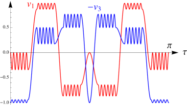
Figure 1. The functions $v_{\alpha}(\tau)$.

the functions $v_{\alpha}(\tau)$ are plotted.

Acknowledgments: We would like to thank Olaf Müller, Karolin Sporrer, Jan-Hendrik Treude and the referees for helpful discussions and comments.

References

- [1] C. Bär, N. Ginoux, and F. Pfäffle, Wave Equations on Lorentzian Manifolds and Quantization, ESI Lectures in Mathematics and Physics, European Mathematical Society (EMS), Zürich, 2007.
- [2] H. Baum, Spinor structures and Dirac operators on pseudo-Riemannian manifolds, Bull. Polish Acad. Sci. Math. 33 (1985), no. 3-4, 165–171.
- [3] A.N. Bernal and M. Sánchez, On smooth Cauchy hypersurfaces and Geroch’s splitting theorem, arXiv:gr-qc/0306108, Comm. Math. Phys. 243 (2003), no. 3, 461–470.
- [4] by same author, Smoothness of time functions and the metric splitting of globally hyperbolic spacetimes, Comm. Math. Phys. 257 (2005), no. 1, 43–50.
- [5] J.D. Bjorken and S.D. Drell, Relativistic Quantum Mechanics, McGraw-Hill Book Co., New York, 1964.
- [6] J. Bognár, Indefinite Inner Product Spaces, Springer-Verlag, New York, 1974, Ergebnisse der Mathematik und ihrer Grenzgebiete, Band 78.
- [7] J. Dimock, Dirac quantum fields on a manifold, Trans. Amer. Math. Soc. 269 (1982), no. 1, 133–147.
- [8] F. Finster, Definition of the Dirac sea in the presence of external fields, arXiv:hep-th/9705006, Adv. Theor. Math. Phys. 2 (1998), no. 5, 963–985.
- [9] by same author, The Principle of the Fermionic Projector, hep-th/0001048, hep-th/0202059, hep-th/0210121, AMS/IP Studies in Advanced Mathematics, vol. 35, American Mathematical Society, Providence, RI, 2006.
- [10] by same author, Causal variational principles on measure spaces, arXiv:0811.2666 [math-ph], J. Reine Angew. Math. 646 (2010), 141–194.
- [11] by same author, A formulation of quantum field theory realizing a sea of interacting Dirac particles, arXiv:0911.2102 [hep-th], Lett. Math. Phys. 97 (2011), no. 2, 165–183.
- [12] F. Finster and A. Grotz, The causal perturbation expansion revisited: Rescaling the interacting Dirac sea, arXiv:0901.0334 [math-ph], J. Math. Phys. 51 (2010), 072301.
- [13] by same author, A Lorentzian quantum geometry, arXiv:1107.2026 [math-ph], Adv. Theor. Math. Phys. 16 (2012), no. 4, 1197–1290.
- [14] F. Finster, A. Grotz, and D. Schiefeneder, Causal fermion systems: A quantum space-time emerging from an action principle, arXiv:1102.2585 [math-ph], Quantum Field Theory and Gravity (F. Finster, O. Müller, M. Nardmann, J. Tolksdorf, and E. Zeidler, eds.), Birkhäuser Verlag, Basel, 2012, pp. 157–182.
- [15] F. Finster and C. Hainzl, A spatially homogeneous and isotropic Einstein-Dirac Cosmology, arXiv:1101.1872 [math-ph], J. Math. Phys. 52 (2011), 042501.
- [16] F. Finster and M. Reintjes, The Dirac equation and the normalization of its solutions in a closed Friedmann-Robertson-Walker universe, arXiv:0901.0602 [math-ph], Classical Quantum Gravity 26 (2009), no. 10, 105021.
- [17] by same author, A non-perturbative construction of the fermionic projector on globally hyperbolic manifolds II – Space-times of infinite lifetime, arXiv:1312.7209 [math-ph], to appear in Adv. Theor. Math. Phys. (2016).
- [18] F. Finster and J. Tolksdorf, Perturbative description of the fermionic projector: Normalization, causality and Furry’s theorem, arXiv:1401.4353 [math-ph], J. Math. Phys. 55 (2014), no. 5, 052301.
- [19] S.W. Hawking and G.F.R. Ellis, The Large Scale Structure of Space-Time, Cambridge University Press, London, 1973.
- [20] L. Hörmander, The Analysis of Linear Partial Differential Operators. I, second ed., Grundlehren der Mathematischen Wissenschaften, vol. 256, Springer-Verlag, Berlin, 1990.
- [21] F. John, Partial Differential Equations, fourth ed., Applied Mathematical Sciences, vol. 1, Springer-Verlag, New York, 1991.
- [22] H. Langer, Spectral functions of definitizable operators in Krein spaces, Functional Analysis (Dubrovnik, 1981), Lecture Notes in Math., vol. 948, Springer, Berlin, 1982, pp. 1–46.
- [23] H.B. Lawson, Jr. and M.-L. Michelsohn, Spin Geometry, Princeton Mathematical Series, vol. 38, Princeton University Press, Princeton, NJ, 1989.
- [24] O. Müller and M. Sánchez, Lorentzian manifolds isometrically embeddable in , Trans. Amer. Math. Soc. 363 (2011), no. 10, 5367–5379.
- [25] M. Reed and B. Simon, Methods of Modern Mathematical Physics. IV, Analysis of operators, Academic Press, New York, 1978.
- [26] by same author, Methods of Modern Mathematical Physics. I, Functional analysis, second ed., Academic Press Inc., New York, 1980.
- [27] B. Thaller, The Dirac Equation, Texts and Monographs in Physics, Springer-Verlag, Berlin, 1992.