Complexity Estimates for Two Uncoupling Algorithms

Abstract

Uncoupling algorithms transform a linear differential system of first order into one or several scalar differential equations. We examine two approaches to uncoupling: the cyclic-vector method (CVM) and the Danilevski-Barkatou-Zürcher algorithm (DBZ). We give tight size bounds on the scalar equations produced by CVM, and design a fast variant of CVM whose complexity is quasi-optimal with respect to the output size. We exhibit a strong structural link between CVM and DBZ enabling to show that, in the generic case, DBZ has polynomial complexity and that it produces a single equation, strongly related to the output of CVM. We prove that algorithm CVM is faster than DBZ by almost two orders of magnitude, and provide experimental results that validate the theoretical complexity analyses.

Categories and Subject Descriptors:
I.1.2 [Computing Methodologies]: Symbolic and Algebraic Manipulations — Algebraic Algorithms

General Terms: Algorithms, Theory.

Keywords: Danilevski-Barkatou-Zürcher algorithm, gauge equivalence, uncoupling, cyclic-vector method, complexity.

1 Introduction

1.1 Motivation

Uncoupling is the transformation of a linear differential system of first order, $Y^{\prime}=MY$, for a square matrix $M$ with coefficients in a rational-function field $\mathbb{K}(X)$ of characteristic zero, into one or several scalar differential equations $y^{(n)}=c_{n-1}y^{(n-1)}+\dots+c_{0}y$, with coefficients $c_{i}$ in $\mathbb{K}(X)$. This change of representation makes it possible to apply algorithms that input scalar differential equations to systems.

In the present article, we examine two uncoupling algorithms: the cyclic-vector method (CVM) [24, 10, 8] and the Danilevski-Barkatou-Zürcher algorithm (DBZ) [12, 5, 30, 6]. While CVM always outputs only one equivalent differential equation, DBZ can decompose the system into several differential equations. This makes us consider two scenarios: the generic case corresponds to situations in which DBZ does not split the system into uncoupled equations, whereas in the general case, several equations can be output.

For some applications, getting several differential equations is more desirable than a single one. Besides, although the complexity of CVM is rarely discussed, its output is said to be “very complicated” in comparison to other uncoupling methods [18, 5, 30, 2, 16]. For these reasons, CVM has had bad reputation. Because of this general belief, uncoupling algorithms have not yet been studied from the complexity viewpoint. The lack and need of such an analysis is however striking when one considers, for instance, statements like We tried to avoid […] cyclic vectors, because we do not have sufficiently strong statements about their size or complexity in a recent work on Jacobson forms [17]. One of our goals is a first step towards filling this gap and rehabilitating CVM.

1.2 Contribution

In relation to the differential system $Y^{\prime}=MY$, a classical tool of differential algebra is the map $\delta$, defined at a matrix or a row vector $u$ by $\delta(u)=uM+u^{\prime}$. A common objective of both CVM and DBZ, explicitly for the former and implicitly for the latter, as we shall prove in the present article, is to discover a basis $P$ of $\mathbb{K}(X)^{n}$ with respect to which the matrix of the application $\delta$ is very simple. This matrix is the matrix $P[M]$ defined in §1.5. In contrast with CVM, which operates only on $P$, DBZ operates only on $P[M]$ by performing pivot manipulations without considering $P$. An important part of our contribution is to provide an algebraic interpretation of the operations in DBZ in terms of transformations of the basis $P$ (§3.1 and §3.2).

More specifically, we analyse the degree of the outputs from CVM and DBZ, so as to compare them. Interestingly enough, an immediate degree analysis of (the first, generically dominating part of) DBZ provides us with a pessimistic exponential growth (§3.3). We prove that this estimate is far from tight: the degree growth is in fact only quadratic (Theorem 12). Surprising simplifications between numerators and denominators explain the result. This leads to the first complexity analysis of DBZ. It appears that, in contradiction to the well-established belief, DBZ and CVM have the same output on generic input systems (Theorem 13).

With respect to complexity, another surprising contribution of our work is that both CVM and DBZ have polynomial complexity in the generic case. Combining results, we design a fast variant of CVM (Theorem 8). Even more surprisingly, it turns out that this fast CVM has better complexity ($\approx n^{\theta+1}d$, for $2\leq\theta\leq 3$) than DBZ ($\approx n^{5}d$), when applied to systems of size $n$ and degree $d$. As the output size is proved to be generically asymptotically proportional to $n^{3}d$, our improvement of CVM is quasi-optimal with respect to the output size.

Another uncoupling algorithm is part of the work in [1]. We briefly analyse its complexity in §3.5 and obtain the same complexity bound as for DBZ (Theorem 17).

Our results remain valid for large positive characteristic. They are experimentally well corroborated in §4.

1.3 Previous work

Uncoupling techniques have been known for a long time; CVM can be traced back at least to Schlesinger [24, p. 156–160]. Loewy [20, 21] was seemingly the first to prove that every square matrix over an ordinary differential field of characteristic zero is gauge-similar to a companion matrix.

That a linear system of first order is equivalent to several scalar linear equations is a consequence of Dickson’s [14, p. 173–174] and Wedderburn’s [29, Th. 10.1] algorithmic results on the Smith-like form of matrices with entries in non-commutative domains; see also [23, Chap III, Sec. 11]. Its refinement nowadays called Jacobson form [19, Th. 3 & 4] implies equivalence to a single scalar equation. This approach was further explored in [15, §6] and [11, 3].

Cope [10, §6] rediscovered Schlesinger’s CVM, and additionally showed that for a system of $n$ equations over $\mathbb{K}(X)$, one can always choose a polynomial cyclic vector of degree less than $n$ in $X$. A generalisation to arbitrary differential fields was given in [8, §7]. The subject of differential cyclic vectors gained a renewed interest in the 1970’s, starting from Deligne’s non-effective proof [13, Ch. II, §1]. An effective version, with no restriction on the characteristic, was given in [8, §3]. CVM has bad reputation, its output being said to have very complicated coefficients [18, 5, 2]. However, ad-hoc examples apart, very few degree bounds and complexity analyses are available [9, §2]. The few complexity results we are aware of [8, 16] only measure operations in $\mathbb{K}(X)$, and do not take degrees in $X$ into account.

Barkatou [5] proposed an alternative uncoupling method reminiscent of Danilevski’s algorithm for computing weak Frobenius forms [12]. Danilevski’s algorithm was also generalised by Zürcher [30]; see also [6, §5]. This is what we call DBZ, for Danilevski, Barkatou, and Zürcher. Various uncoupling algorithms are described and analysed in [16, 22], including the already mentioned algorithm from [1].

1.4 Notation and Conventions

Algebraic Structures and Complexity. Let $\mathbb{K}$ denote a field of characteristic zero, $\mathbb{K}_{d}[X]$ the set of polynomials of degree at most $d$, and $\mathcal{M}_{n}(S)$ and $\mathcal{M}_{1,n}(S)$, respectively, the sets of square matrices of dimension $n\times n$ and of row vectors of dimension $n$, each with coefficients in some set $S$. The arithmetic size of a matrix in $\mathcal{M}_{n}(\mathbb{K}(X))$ is the number of elements of $\mathbb{K}$ in its dense representation.

We consider the arithmetic complexity of algorithms, that is, the number of operations they require in the base field $\mathbb{K}$. For asymptotic complexity, we employ the classical notation ${\mathcal{O}}({\cdot})$, $\Omega({\cdot})$, and $\Theta({\cdot})$, as well as the notation $g=\tilde{\mathcal{O}}(f)$ if there exists $k$ such that $g/f={\mathcal{O}}(\log^{k}n)$. We denote by $\mathsf{M}(d)$ (resp. $\mathsf{MM}(n,d)$) the arithmetic complexity of the multiplication in $\mathbb{K}_{d}[X]$ (resp. in $\mathcal{M}_{n}(\mathbb{K}_{d}[X])$). When the complexity of an algorithm is expressed in terms of $\mathsf{M}$ and $\mathsf{MM}$, it means that the algorithm can use multiplication (in $\mathbb{K}[X]$ and $\mathcal{M}_{n}(\mathbb{K}[X])$) as “black boxes”. Estimates for $\mathsf{M}(d)$ and $\mathsf{MM}(n,d)$ are summarised in the following table, where $\theta$ is a constant between $2$ and $3$ that depends on the matrix-multiplication algorithm used. For instance, $\theta=3$ for the schoolbook algorithm, and $\theta=\log_{2}(7)\approx 2.807$ for Strassen’s algorithm [27]. The current tightest upper bound, due to Vassilevska Williams [28], is $\theta<2.3727$.

Structure Notation Naive Fast Size $\mathbb{K}$ – 1 1 1 $\mathbb{K}_{d}[X]$ $\mathsf{M}(d)$ ${\mathcal{O}}(d^{2})$ $\tilde{\mathcal{O}}(d)$ [25] $\Theta(d)$ $\mathcal{M}_{n}(\mathbb{K}_{d}[X])$ $\mathsf{MM}(n,d)$ ${\mathcal{O}}(n^{3}d^{2})$ $\tilde{\mathcal{O}}(n^{\theta}d)$  [7] $\Theta(n^{2}d)$

The complexity of an algorithm is said to be quasi-optimal when, assuming $\theta=2$, it matches the arithmetic size of its output up to logarithmic factors. For instance, the algorithms in the table above have quasi-optimal complexity.

Generic Matrices. The notion of genericity is useful to analyse algorithms on inputs that are not “particular”. For parameters in some $\mathbb{K}^{r}$, a property is classically said to be generic if it holds out of the zero set of a non-zero $r$-variate polynomial. To define the notion of generic matrices, we identify $M\in\mathcal{M}_{n}(\mathbb{K}_{d}[X])$ with the family $\{m_{i,j,k}\}$, indexed by $1\leq i,j\leq n,\ 0\leq k\leq d$, of its coefficients in $\mathbb{K}$.

Conventions. In this text, $M$ is always the input of the uncoupling algorithms. It is assumed to be a matrix in $q(X)^{-1}\mathcal{M}_{n}(\mathbb{K}_{d}[X])$ with $q(X)\in\mathbb{K}_{d}[X]$. It defines $\delta$ on a matrix or a row vector $u$ by $\delta(u)=uM+u^{\prime}$.

For a matrix $A$, we respectively denote its $i$th row and $j$th column by $A_{i,\ast}$ and ${A_{\ast,j}}$. We write $\operatorname{\sf VJoin}(r^{(1)},\ldots,r^{(n)})$ for the matrix $A$ such that for all $i$, $A_{i,\ast}=r^{(i)}$. We define the rows $e_{i}$ by $I_{n}=\operatorname{\sf VJoin}(e_{1},\dots,e_{n})$.

A square matrix $C$ is said to be companion if beside zero coefficients, it has $1$s on its upper diagonal and arbitrary coefficients on its last row, $c=(c_{0},\dots,c_{n-1})$. Thus:

$$C=\operatorname{\sf VJoin}(e_{2},\dots,e_{n-1},c).$$ (1)

We say $A$ has its $i$th row in companion shape if $A_{i,\ast}=e_{i+1}$.

We write $\operatorname{diag}(B^{(1)},\dots,B^{(n)})$ for a diagonal block matrix given by square blocks $B^{(i)}$.

Degrees of rational functions and matrices. In the present paper, the degree of a rational function is the maximum of the degrees of its numerator and denominator. The degree of a vector or a matrix with rational-function coefficients is the maximum of the degrees of its coefficients. The following lemma expresses the generic degrees encountered when solving a generic matrix.

Lemma 1

Let $A$ be a matrix in $\mathcal{M}_{n}(\mathbb{K}[X])$. Define $a_{i}$ as $\deg(A_{i,\ast})$ and $D$ as $\sum_{i}a_{i}$. Then, $\deg(\det(A))\leq D$ and, for all i, $\deg(\det(A){(A^{-1})_{\ast,i}})\leq D-a_{i}$. When $A$ is generic with $\deg(A_{i,\ast})=a_{i}$ for all $i$, those bounds are reached.

Proof.

Proofs use classical techniques and are omitted. We simply observe that $\operatorname{diag}(x^{a_{1}},\dots,x^{a_{n}})\,N$ reaches the announced bounds when $N\in\mathcal{M}_{n}(\mathbb{K}\smallsetminus\{0\})$ and $\det N\neq 0$. ∎

1.5 Companion matrices and uncoupling

For an invertible matrix $P$, let us perform the change of unknowns $Z=PY$ in a system $Y^{\prime}=MY$. Then, $Z^{\prime}=P\,Y^{\prime}+P^{\prime}Y=(P\,M+P^{\prime})P^{-1}Z$. The system is therefore equivalent to $Z^{\prime}=P[M]\,Z$ where $P[M]$ denotes $(P\,M+P^{\prime})P^{-1}$, in the sense that the solutions of both systems, whether meromorphic or rational, are in bijection under $P$.

We call gauge transformation of a matrix $A$ by an invertible matrix $P$ the matrix $P[A]=(P\,A+P^{\prime})P^{-1}$. When $B=P[A]$, we say that $A$ and $B$ are gauge-similar. The gauge-similarity relation is transitive since $P[Q[A]]=(P\,Q)[A]$. With the notation introduced above, $P[M]=\delta(P)\,P^{-1}$.

The following folklore theorem relates the solutions of a system with the solutions of the uncoupled equations obtained from a suitable gauge-similar system: it states that, to uncouple the system $Y^{\prime}=MY$, it suffices to find an invertible matrix $P$ such that $P[M]$ is in diagonal companion block form. This is the main motivation for uncoupling. We omit its proof, as it has similarity with the proofs in §2.1, and because we use no consequence of it later in this article. (We write $\partial f$ instead of $f^{\prime}$ for derivations.)

Theorem 2

Let $P$ be an invertible matrix such that

$$P[M]=\operatorname{diag}(C^{(1)},\dots,C^{(t)})$$ (2)

with $C^{(i)}$ companion of dimension $k_{i}$. Denote the last row of $C^{(i)}$ by $\bigl{(}c^{(i)}_{0},\dots,c^{(i)}_{k_{i}-1}\bigr{)}$. Then, $\partial Y=M\,Y$ if and only if

$$PY=\operatorname{\sf VJoin}(Z^{(1)},\ldots,Z^{(t)})$$

where $Z^{(i)}=\bigl{(}z^{(i)},\partial z^{(i)},\dots,\partial^{k_{i}-1}z^{(i)}\bigr{)}^{T}$ and

$$\partial^{k_{i}}z^{(i)}=c^{(i)}_{k_{i}-1}\partial^{k_{i}-1}z^{(i)}+\dots+c^{(i)}_{0}z^{(i)}.$$

2 Cyclic-vector method

Two versions of CVM are available, depending on how the first row of $P$ is obtained: a version ProbCV picks this first row at random, and thus potentially fails, but with tiny probability; a deterministic version DetCV computes a first row in such a way that the subsequent process provably cannot fail. In both cases, CVM produces no non-trivial diagonal companion block decomposition but only one block.

We present the randomised CVM only, before analysing the degree of its output and giving a fast variant.

2.1 Structure theorems

Let $\Delta^{k}(u)$ denote the matrix $\operatorname{\sf VJoin}(u,\delta(u),\ldots,\delta^{k-1}(u))$ of dimension $k\times n$. The diagonal companion block decomposition (2) is based on the following folklore result.

Lemma 3

Let $P$ be an invertible matrix. Then, there exists a companion matrix $C$ of dimension $k$ such that

$$P[M]=\left(\begin{smallmatrix}C&0\\ \ast&\ast\end{smallmatrix}\right)$$ (3)

if and only if there exists a vector $u$ such that $P=\left(\begin{smallmatrix}\Delta^{k}(u)\\ \ast\end{smallmatrix}\right)$ and $\delta^{k}(u)\in\operatorname{span}\bigl{(}u,\delta(u),\ldots,\delta^{k-1}(u)\bigr{)}$.

Proof.

Set $\left(\begin{smallmatrix}U\\ R\end{smallmatrix}\right):=P$ where $U$ has $k$ rows. Equality (3) is equivalent to $\delta\left(\begin{smallmatrix}U\\ R\end{smallmatrix}\right)=\left(\begin{smallmatrix}C&0\\ \ast&\ast\end{smallmatrix}\right)\left(\begin{smallmatrix}U\\ R\end{smallmatrix}\right)$, then with $\delta(U)=C\,U$. This can be rewritten:

$$\operatorname{\sf VJoin}(\delta(U_{1,\ast}),\ldots,\delta(U_{k,\ast}))=\operatorname{\sf VJoin}(U_{2,\ast},\ldots,U_{k,\ast},C_{k,\ast}U).$$

Set $u$ to the first row of $U$. This equation is satisfied if and only if $U=\Delta^{k}(u)$ and $\delta^{k}(u)\in\operatorname{span}(\Delta^{k}(u))$. ∎

The following corollaries for partial companion decomposition and diagonal companion block decomposition are proved in a very similar fashion to the preceding lemma. They will be used for the analysis of CVM and DBZ.

Corollary 4

Let $P$ be an invertible matrix. Then, $P[M]$ has its first $k-1$ rows in companion shape if and only if there exists a row vector $u$ such that $P=\left(\begin{smallmatrix}\Delta^{k}(u)\\ \ast\end{smallmatrix}\right)$.

Corollary 5

Let $P$ be an invertible matrix and $\{C^{(i)}\}_{1\leq i\leq t}$ a family of companion matrices of dimension $k_{i}$. Then,

$$P[M]=\operatorname{diag}(C^{(1)},\ldots,C^{(t)})$$

if and only if there exist $t$ row vectors $\{u^{(i)}\}_{1\leq i\leq t}$ such that $P=\operatorname{\sf VJoin}(\Delta^{k_{1}}(u^{(1)}),\ldots,\Delta^{k_{t}}(u^{(t)}))$ and for all $i$, $\delta^{k_{i}}(u^{(i)})$ is in $\operatorname{span}(\Delta^{k_{i}}(u^{(i)}))$.

2.2 Classical algorithms for cyclic vectors

The name CVM comes from the following notion.

Definition

A cyclic vector is a row vector $u\in\mathbb{K}(X)^{n}$ for which the matrix $\Delta^{n}(u)$ is invertible, or, equivalently, such that the cyclic module generated by $u$ over $\mathbb{K}(X)\langle\delta\rangle$ is the full vector space $\mathcal{M}_{1,n}\bigl{(}\mathbb{K}(X)\bigr{)}$ of row vectors.

The next folklore method [5, 8] is justified by Theorem 6 below, which means that CVTrial will not fail too often.

Algorithm 1 CVTrial: Testing if a vector is a cyclic vector

Input: $M\in q(X)^{-1}\mathcal{M}_{n}(\mathbb{K}_{d}[X])$ and $u\in\mathcal{M}_{1,n}(\mathbb{K}_{n-1}[X])$
Output: $P$, $C$ with $C$ companion and $\delta(P)P^{-1}=C$

1:  set $P$ to the square zero matrix of dimension $n$

2:  $P_{1,\ast}:=u$

3:  for $i=1$ to $n-1$, do $P_{i+1,\ast}:=\delta(P_{i,\ast})$

4:  if $P$ is not invertible, return “Not a cyclic vector”

5:  $C:=\delta(P)P^{-1}$

6:  return $(P,C)$

Theorem 6

[10, 8] When $u$ is generic of degree less than $n$, the matrix $P=\Delta^{n}(u)$ is invertible.

Proof.

It is proved in [10, 8] that every matrix $M$ admits a cyclic vector $u$ of degree less than $n$. Then, $\det({\cdot})$ is a non-zero polynomial function of the matrix coefficients. ∎

In ProbCV, $u$ is chosen randomly, leading to a Las Vegas algorithm for finding a cyclic vector. The proof above refers to the theorem that every matrix $M$ admits a cyclic vector. Churchill and Kovacic give in [8] a good survey of this subject. They also provide an algorithm that we denote DetCV that takes as input a square matrix $M$ and deterministically outputs a cyclic vector $u$. The arithmetic complexity of this algorithm is polynomial, but worse than that of ProbCV.

2.3 Degree analysis and fast algorithm

CVTrial computes two matrices, $P$ and $C$, whose sizes we now analyse. We shall find the common bound ${\mathcal{O}}(n^{3}d)$. When $u\in\mathcal{M}_{1,n}(\mathbb{K}_{n-1}[X])$ is generic, this bound is reached. The size $\Theta(n^{3}d)$ of the output of CVTrial is then a lower bound on the complexity of any algorithm specifying CVM. After the remark that the complexity of the simple algorithm is above this bound, we give a fast algorithm.

We start by bounding the degree of the matrix $\Delta^{n}(u)$. Following the result of Churchill and Kovacic, we make the assumption that $\deg(u)$ is less than $n$.

Lemma 7

The row vector $q^{k}\delta^{k}(u)$ consists of polynomials of degree at most $\deg(u)+kd$.

Proof.

The proof proceeds by induction after noting that $q^{k+1}\delta^{k+1}=q(\delta q^{k}-kq^{k-1}q^{\prime})\delta^{k}=(q\delta-kq^{\prime})q^{k}\delta^{k}$. ∎

We list further bounds on degrees and arithmetic sizes, some of which are already in [9, §2]:

	Degree	Arithmetic size
$P$	$\deg(u)+(n-1)d$	${\mathcal{O}}(n^{3}d+n^{2}\deg(u))$
$P^{-1}$	$n\deg(u)+\frac{n(n-1)}{2}d$	${\mathcal{O}}(n^{4}d+n^{3}\deg(u))$
$\delta^{n}(u)$	$\deg(u)+nd$	${\mathcal{O}}(n^{2}d+n\deg(u))$
$C$	$n\deg(u)+\frac{n(n+1)}{2}d$	${\mathcal{O}}(n^{3}d+n^{2}\deg(u))$

Theorem 8

Algorithm CVTrial implements CVM in quasi-optimal complexity $\tilde{\mathcal{O}}(n^{\theta+1}d)$.

Proof.

At Step 3, CVTrial computes $\delta(P_{i,\ast})=P_{i,\ast}M+P_{i,\ast}^{\prime}$ for successive $i$’s. Addition and derivation have softly linear complexity, so we focus on the product $P_{i,\ast}M$. Computing it by a vector-matrix product would have complexity $\Omega(n^{2}id)$ and the complexity of the loop at Step 3 would then be $\Omega(n^{4}d)$. The row $P_{i,\ast}$ has higher degree than $M$, so the classical idea to make it a matrix to balance the product applies. Let $A_{k}\in\mathbb{K}_{d}[X]^{n}$ be the rows defined by $P_{i,\ast}=\sum_{k=0}^{n-1}A_{k}X^{kd}$, and $A:=\operatorname{\sf VJoin}(A_{0},\dots,A_{n-1})$. The product $AM$ is computed in complexity ${\mathcal{O}}(\mathsf{MM}(n,d))$, and $P_{i,\ast}M$ is reconstructed in linear complexity, thus performing the whole loop in complexity ${\mathcal{O}}(n\,\mathsf{MM}(n,d))$.

Only the last row $\delta^{n}(u)P^{-1}$ of $C$ needs to be computed at Step 5, and the size $\Theta(n^{4}d)$ of $P^{-1}$ bans the computation of $P^{-1}$ from any low complexity algorithm. $C$ can be computed in complexity $\tilde{\mathcal{O}}(\mathsf{MM}(n,nd))$. This is achieved by solving $PY=\delta^{n}(u)$ by Storjohann’s algorithm [26], which inputs $\delta^{n}(u)$ and $P$, of degree $\Theta(nd)$, and outputs the last row $\delta^{n}(u)\,P^{-1}$ of $C$ in ${\mathcal{O}}(\mathsf{MM}(n,nd)\log(nd))$ operations. ∎

3 The Danilevski-Barkatou-
Zürcher algorithm

We begin this section with a description of algorithm DBZ, before a naive analysis that gives exponential bounds. Experiments show a polynomial practical complexity, whence the need for a finer analysis. To obtain it, we develop an algebraic interpretation of the algorithm.

3.1 Description of the algorithm

The input to DBZ is a matrix $M\in\mathcal{M}_{n}(\mathbb{K}(X))$; its output $(P,C^{(1)},\ldots,C^{(t)})$ satisfies $P[M]=\operatorname{diag}(C^{(1)},\dots,C^{(t)})$ for companion matrices $C^{(i)}$. DBZ iterates over $P[M]$ to make it progressively diagonal block-companion. To do so, three sub-algorithms are used, $\textsf{DBZ}^{\text{I}}$, $\textsf{DBZ}^{\text{II}}$, and $\textsf{DBZ}^{\text{III}}$, in order to achieve special intermediate forms for $P[M]$. These forms, respectively Shape (I), (II), and (III), are:

$$\begin{pmatrix}C&0\\ \alpha&\beta\end{pmatrix},\quad\begin{pmatrix}C&\begin{smallmatrix}0&\cdots&0\\ \vdots&&\vdots\\ 0&\cdots&0\end{smallmatrix}\\ \begin{smallmatrix}v&\begin{smallmatrix}0&\cdots&0\\ \vdots&&\vdots\\ 0&\cdots&0\end{smallmatrix}\end{smallmatrix}&\beta\end{pmatrix},\quad\begin{pmatrix}\ast&\begin{smallmatrix}1&0&\cdots&0\end{smallmatrix}&\begin{smallmatrix}\ast&\cdots&\ast\end{smallmatrix}\\ \begin{smallmatrix}0\\ \vdots\\ 0\end{smallmatrix}&C&\begin{smallmatrix}0&\cdots&0\\ \vdots&&\vdots\\ 0&\cdots&0\end{smallmatrix}\\ \begin{smallmatrix}\ast\\ \vdots\\ \ast\end{smallmatrix}&\begin{smallmatrix}0&\cdots&\cdots&0\\ \vdots&&&\vdots\\ 0&\cdots&\cdots&0\end{smallmatrix}&\begin{smallmatrix}\ast&\cdots&\ast\\ \vdots&&\vdots\\ \ast&\cdots&\ast\end{smallmatrix}\end{pmatrix},$$

​​where in each case $C$ denotes a companion matrix, $v$ is a column vector, $\alpha,\beta$ are general matrices, and $\beta$ is square.

In the course of DBZ, first, $\textsf{DBZ}^{\text{I}}$ computes $P^{\text{I}}$ and $M^{\text{I}}$ such that $P^{\text{I}}[M]=M^{\text{I}}$ has Shape (I). If $M^{\text{I}}=C$ is companion — that is, if $\alpha$ and $\beta$ do not occur — then DBZ returns $(P^{\text{I}},M^{\text{I}})$. If not, at this point, DBZ has obtained a first companion block $C$ and we would hope that $\alpha$ is zero to apply DBZ recursively to $\beta$. So, in general, DBZ tries to cancel $\alpha$, by appealing to $\textsf{DBZ}^{\text{II}}$ to compute $P^{\text{II}}$ and $M^{\text{II}}$ such that $P^{\text{II}}[M^{\text{I}}]=M^{\text{II}}$ has Shape (II). If the obtained $v$ is zero, then DBZ can go recursively to $\beta$.

If not, DBZ seems to have failed and restarts on a matrix $P^{\text{III}}[M^{\text{II}}]=M^{\text{III}}$ with Shape (III), which ensures $\textsf{DBZ}^{\text{I}}$ can treat at least one more row than previously (as proved in [6]). Therefore, the algorithm does not loop forever. The matrix $M^{\text{III}}$ on which DBZ starts over and the differential change of basis $P^{\text{III}}$ associated are computed by $\textsf{DBZ}^{\text{III}}$.

Algorithm 2 DBZ (Danilevski-Barkatou-Zürcher)

Input: $M\in\mathcal{M}_{n}(\mathbb{K}(X))$
Output: $(P,C^{(1)},\ldots,C^{(t)})$ with $C^{(i)}$ companion matrices and $P[M]=\operatorname{diag}(C^{(1)},\ldots,C^{(t)})$

1:  $(P^{\text{I}},M^{\text{I}}):=\text{$\textsf{DBZ}^{\text{I}}$}(M)$

2:  if $M^{\text{I}}$ is companion then return$(P^{\text{I}},M^{\text{I}})$

3:  $(P^{\text{II}},M^{\text{II}}):=\text{$\textsf{DBZ}^{\text{II}}$}(M^{\text{I}})$

4:  $\left(\begin{smallmatrix}C&0\\ \begin{smallmatrix}v&0\end{smallmatrix}&\beta\end{smallmatrix}\right):=M^{\text{II}}$ where $v\in\mathcal{M}_{n-k,1}(\mathbb{K}(X))$

5:  if $v=0$ then

6:      $(P,C^{(1)},\ldots,C^{(t)}):=\text{{DBZ}}(\beta)$

7:      return $(\operatorname{diag}(I_{k},P)P^{\text{II}}P^{\text{I}},C,C^{(1)},\ldots,C^{(t)})$

8:  $(P^{\text{III}},M^{\text{III}}):=\text{$\textsf{DBZ}^{\text{III}}$}(M^{\text{II}})$

9:  $(P,C^{(1)},\ldots,C^{(t)}):=\text{{DBZ}}(M^{\text{III}})$

10:  return $(PP^{\text{III}}P^{\text{II}}P^{\text{I}},C^{(1)},\ldots,C^{(t)})$

3.2 Description of the sub-algorithms

We now describe $\textsf{DBZ}^{\text{I}}$, $\textsf{DBZ}^{\text{II}}$, and $\textsf{DBZ}^{\text{III}}$ in more details. By $E_{i,j}(t)$, we denote the matrix obtained after replacing by $t$ the $(i,j)$ coefficient in the identity matrix $I_{n}$, and by $E_{i}(u)$ the matrix obtained after replacing the $i$th row by the row vector $u$ in $I_{n}$. Let $\mathsf{Inv}^{(j,n)}$ denote the matrix obtained from $I_{n}$ after exchanging the $j$th and $n$th rows. Set $\mathsf{Rot}=\operatorname{\sf VJoin}(e_{n},e_{1},\ldots,e_{n-1})$.

The algorithms developed below rely on a common Pivot subtask, which inputs $(M,P,T)\in\mathcal{M}_{n}(\mathbb{K}(X))^{3}$ with invertible $P$ and $T$, and outputs the update of $(M,P)$ under $T$. This really behaves like a Gauge transformation, changing $(M,P)$ to $\bigl{(}T[M],TP\bigr{)}$. This modification of $M$ and $P$ only ensures the invariant $M=P[M_{\text{initial}}]$.

$\textsf{DBZ}^{\text{I}}$ inputs $M$ and outputs the tuple of matrices $(P^{\text{I}},M^{\text{I}})$ with $M^{\text{I}}$ in Shape (I). It starts with $M^{\text{I}}=M$ and modifies its rows one by one. At the $i$th iteration of the loop (Step 2), the matrix $M^{\text{I}}$ has its first $i-1$ rows in companion form. To put the $i$th row in companion form, $\textsf{DBZ}^{\text{I}}$ sets $M^{\text{I}}_{i+1,i+2}$ to 1 (Step 6), and uses it as a pivot to cancel the other coefficients of the row (loop at Step 7).

Algorithm 3 $\textsf{DBZ}^{\text{I}}$

Input: $M\in\mathcal{M}_{n}(\mathbb{K}(X))$
Output: $(P^{\text{I}},M^{\text{I}})$ with $M^{\text{I}}$ in Shape (I) and $P^{\text{I}}[M]=M^{\text{I}}$

1:  $(P^{\text{I}},M^{\text{I}}):=(I,M)$

2:  for $i=1$ to $n-1$ do

3:      $r:=\min\bigl{(}\{j\ |\ M^{\text{I}}_{i,j}\neq 0\ \text{and}\ j>i\}\cup\{n+1\}\bigr{)}$

4:      if $r=n+1$ then return $(P^{\text{I}},M^{\text{I}})$

5:      $(M^{\text{I}},P^{\text{I}}):=\textsf{Pivot}(M^{\text{I}},P^{\text{I}},\mathsf{Inv}^{(i+1,r)})$

6:      $(M^{\text{I}},P^{\text{I}}):=\textsf{Pivot}(M^{\text{I}},P^{\text{I}},E_{i+1,i+1}(M^{\text{I}}_{i,i+1})^{-1})$

7:      for $j=1$ to $n$ with $j\neq i+1$ do

8:          $(M^{\text{I}},P^{\text{I}}):=\textsf{Pivot}(M^{\text{I}},P^{\text{I}},E_{i+1,j}(-M^{\text{I}}_{i,j}))$

9:  return $(P^{\text{I}},M^{\text{I}})$

If $M^{\text{I}}_{i+1,i+2}=0$ and there is a non-zero coefficient farther on the row, then the corresponding columns are inverted at Step 5 and $\textsf{DBZ}^{\text{I}}$ goes on. If there is no such coefficient, the matrix has reached Shape (I) and is returned at Step 4.

$\textsf{DBZ}^{\text{II}}$ inputs $M^{\text{I}}$ and outputs a tuple $(P^{\text{II}},M^{\text{II}})$ with $M^{\text{II}}$ in Shape (II). At Step 3, it cancels the columns of the lower-left block of $M^{\text{I}}$ one by one, from the last one to the second one, using the 1’s of $C$ as pivots. At the $\ell$th iteration, the lower-left block of $M^{\text{I}}$ ends with $\ell$ zero columns.

Algorithm 4 $\textsf{DBZ}^{\text{II}}$

Input: $M^{\text{I}}$ in Shape (I)
Output: $(P^{\text{II}},M^{\text{II}})$ in Shape (II) such that $P^{\text{II}}[M^{\text{I}}]=M^{\text{II}}$

1:  $k:=$ size of the companion block of $M^{\text{I}}$

2:  $(P^{\text{II}},M^{\text{II}}):=(I,M^{\text{I}})$

3:  for $j=k$ down to 2 do

4:      for $i=k+1$ to $n$ do

5:          $(M^{\text{II}},P^{\text{II}}):=\textsf{Pivot}(M^{\text{II}},P^{\text{II}},E_{i,j-1}(-M^{\text{II}}_{i,j}))$

6:  return $(P^{\text{II}},M^{\text{II}})$

$\textsf{DBZ}^{\text{III}}$ inputs $M^{\text{II}}$ with $v$ non-zero and outputs the tuple $(P^{\text{III}},M^{\text{III}})$ with $M^{\text{III}}$ in Shape (III). The transformation of $M$ at Step 3 reverses $v$ to put a non-zero coefficient on the last row of $M^{\text{II}}$. Then it sets it to 1 at Step 4 and uses it as a pivot to cancel the other $v_{j}$’s (Step 6). Finally, at Step 7, a cyclic permutation is applied to the rows and columns: last row becomes first, last column becomes first.

Algorithm 5 $\textsf{DBZ}^{\text{III}}$

Input: $M^{\text{II}}$ in Shape (II), under the constraints $C$ has dimension $k$ and $v\neq 0$
Output: $(P^{\text{III}},M^{\text{III}})$ in Shape (III) where $P^{\text{III}}[M^{\text{II}}]=M^{\text{III}}$

1:  $M^{\text{III}}:=M^{\text{II}}$

2:  $h:=\max\{i\ |\ M^{\text{III}}_{i,1}\neq 0\}$

3:  $(M^{\text{III}},P^{\text{III}}):=\textsf{Pivot}(M^{\text{III}},P^{\text{III}},\mathsf{Inv}^{(h,n)})$

4:  $(M^{\text{III}},P^{\text{III}}):=\textsf{Pivot}(M^{\text{III}},P^{\text{III}},E_{n,n}(1/M^{\text{III}}_{n,1}))$

5:  for $i=k+1$ to $n-1$ do

6:      $(M^{\text{III}},P^{\text{III}}):=\textsf{Pivot}(M^{\text{III}},P^{\text{III}},E_{i,n}(-M^{\text{III}}_{i,1}))$

7:  $(M^{\text{III}},P^{\text{III}}):=\textsf{Pivot}(M^{\text{III}},P^{\text{III}},\mathsf{Rot})$

8:  return $(P^{\text{III}},M^{\text{III}})$

3.3 A naive degree analysis of the generic case

When $M$ is generic, $\textsf{DBZ}^{\text{I}}$ outputs a companion matrix, so DBZ terminates at Step 2 in the generic case with only one companion matrix in the diagonal companion block decomposition. The proof of this fact will be given in §3.4. Therefore, the complexity of $\textsf{DBZ}^{\text{I}}$ is interesting in itself.

A lower bound on this complexity is the degree of its output. We explain here why a naive analysis of $\textsf{DBZ}^{\text{I}}$ only gives an exponential upper bound on this degree.

Let $M^{(i)}$ be the value of $M^{\text{I}}$ just before the $i$th iteration of the loop at Step 2 (in particular, $M^{(1)}=M$), and $M^{(n)}$ the output value. Remark that the matrices involved in the gauge transformations at Steps 6 and 8 commute with one another. Their product is equal to $E_{i+1}(\mathsf{Inv}^{(i+1,r)}[M^{(i)}]_{i,\ast})$.

Lemma 9

If $A\in\mathcal{M}_{n}(\mathbb{K}_{d}[X])$ is a generic matrix with its first $i-1$ rows in companion form and $T=E_{i+1}(A_{i,\ast})$, then $T[A]$ has degree $3d$.

An exponential bound on the output of $\textsf{DBZ}^{\text{I}}$ is easily deduced: $\deg(M^{(n)})\leq 3^{n-1}\deg(M)$. We will dramatically improve this bound in the following section.

3.4 ​​​Algebraic interpretation and better bounds

To prove the announced tight bound, it could in principle be possible to follow the same pattern as in Bareiss’ method [4]: give an explicit form for the coefficients of the transformed matrices $M$, from which the degree analysis becomes obvious. But it proves more fruitful to find a link between CVM and DBZ, and our approach involves almost no computation.

Algorithm DBZ reshapes the input matrix by successive elementary gauge transformations. It completely relies on the shape of $M$, $M^{\text{I}}$, $M^{\text{II}}$, and $M^{\text{III}}$, while the construction of the matrices $P$ is only a side-effect. As illustrated in §3.3, this approach is not well suited for degree analysis.

In this section, we focus on $P$, $P^{\text{I}}$, $P^{\text{II}}$, and $P^{\text{III}}$. It turns out that these matrices allow nice algebraic formulations, leading to sharp degree and complexity analyses of DBZ.

The following lemma, whose omitted proof is immediate from the design of DBZ, provides the complexity of the computation of an elementary gauge transformation.

Lemma 10

If $t\in\mathbb{K}_{d}[X]$ and $M\in\mathcal{M}_{n}(\mathbb{K}_{d}[X])$, then the gauge transformation of $M$ by $E_{i,j}(t)$ can be computed in ${\mathcal{O}}(n\,\mathsf{M}(d))=\tilde{\mathcal{O}}(nd)$ operations in $\mathbb{K}$.

3.4.1 Analysis of $\text{{DBZ}}^{\text{I}}$

We consider an execution of Algorithm $\textsf{DBZ}^{\text{I}}$ on a matrix $M$ of denominator $q$, where $\deg(q)$ and $\deg(qM)$ are equal to $d$. Let $P^{(i)}$ and $M^{(i)}$ be the values of the matrices $P^{\text{I}}$ and $M^{\text{I}}$ when entering the $i$th iteration of the loop at Step 2, and $P^{(n)}$ and $M^{(n)}$ the values they have at Step 9 if this step is reached. Set $k$ to either the last value of $i$ before returning at Step 4 or $n$ if Step 9 is reached. Consequently, the companion block $C$ of $M^{\text{I}}$ has dimension $k$. The use of Algorithm Pivot ensures the invariant $M^{(i)}=P^{(i)}[M]$ for all $i\leq k$.

The following lemma gives the shape of the matrices $P^{(i)}$.

Lemma 11

For each $i$, $P^{(i)}=\operatorname{\sf VJoin}(\Delta^{i}(e_{1}),Q^{(i)})$ for some $Q^{(i)}$ whose rows are in $\{e_{2},\ldots,e_{n}\}$.

Proof.

The first $i-1$ rows of $P^{(i)}[M]$ have companion shape by design of $\textsf{DBZ}^{\text{I}}$. So, by Corollary 4, there exist a vector $u$ and a matrix $Q^{(i)}$ with $P^{(i)}=\operatorname{\sf VJoin}(\Delta^{i}(u),Q^{(i)})$.

We now prove by induction that $P^{(i)}_{1,\ast}=e_{1}$ and that for all $a>i$, $P^{(i)}_{a,\ast}\in\{e_{2},\ldots,e_{n}\}$. First for $i=1$, $P^{(1)}=I$, so the property holds. Now, we assume the property for $P^{(i)}$ and consider the $i$th iteration of the loop at Step 2. For $j\neq i+1$, let $T^{(j)}$ denote the value of the matrix involved in the gauge transformation at Step 8 during the $j$th iteration of the loop at Step 7, and let $T^{(i+1)}$ denote the matrix used at Step 6. Let $r$ denote the integer defined at Step 3.

The transformations of $P$ at Steps 5, 6, and 8 imply $P^{(i+1)}=T^{(n)}\dotsm T^{(i+2)}T^{(i)}\dotsm T^{(1)}T^{(i+1)}\mathsf{Inv}^{(i+1,r)}P^{(i)}$. The first row of each matrix $T^{(j)}$ and each matrix $\mathsf{Inv}^{(i+1,r)}$ is $e_{1}$, so $P^{(i+1)}_{1,\ast}=P^{(i)}_{1,\ast}$ which is, by induction, equal to $e_{1}$.

For each integer $a>i+1$ and each $j$, by definition $T^{(j)}_{a,\ast}=e_{a}$. Therefore, $P^{(i+1)}_{a,\ast}=\mathsf{Inv}^{(i+1,r)}_{a,\ast}P^{(i)}$. Moreover, if $a=r$, then $\mathsf{Inv}^{(i+1,r)}_{a,\ast}$ is equal to $e_{i+1}$; if not, it is equal to $e_{a}$. In both cases, by induction, $\mathsf{Inv}^{(i+1,r)}_{a,\ast}P^{(i)}\in\{e_{2},\ldots,e_{n}\}$. ∎

We are now able to give precise bounds on the degree of the output and the complexity of $\textsf{DBZ}^{\text{I}}$, using Lemma 1.

Theorem 12

Let $k$ be the dimension of the companion block output from $\textsf{DBZ}^{\text{I}}$. The degree of $q^{k-1}P^{(k)}$ is ${\mathcal{O}}(kd)$ and the degree of $\bigl{(}q^{k(k+1)/2}\det(P^{(k)})\bigr{)}M^{(k)}$ is ${\mathcal{O}}(k^{2}d)$. $\textsf{DBZ}^{\text{I}}$ has complexity ${\mathcal{O}}(n^{2}k\,\mathsf{M}(k^{2}d))=\tilde{\mathcal{O}}(n^{2}k^{3}d)$.

It is possible to give more precise bounds on the degrees and even to prove that they are reached in the generic case.

Proof.

By Lemmas 11 and 7, the degrees of the rows of $\operatorname{diag}(1,q,\ldots,q^{i-1},1,\ldots,1)P^{(i)}$ are upper bounded by $(0,d,$ $\ldots,(i-1)d,0,\ldots,0)$. Now Lemma 1 implies that the degree of $q^{i(i-1)/2}\det(P^{(i)}){P^{(i)}}^{-1}$ is ${\mathcal{O}}(i^{2}d)$. By the invariant of Pivot and $P[M]=\delta(P)\,P^{-1}$, $M^{(i)}=\delta(P^{(i)}){P^{(i)}}^{-1}$, we deduce that the lcm of the denominators in $M^{(i)}$ divides $L_{i}:=q^{i(i+1)/2}\det(P^{(i)})$ and that $\deg(L_{i}M^{(i)})$ is in ${\mathcal{O}}(i^{2}d)$. The degrees of the theorem follow for $i=k$.

The computation of $M^{(i+1)}$ from $M^{(i)}$ uses $n$ elementary gauge transformations on $M^{(i)}$, leading by Lemma 10 to a complexity ${\mathcal{O}}(n^{2}\mathsf{M}(i^{2}d))$. The announced complexity for $\textsf{DBZ}^{\text{I}}$ is obtained upon summation over $i$ from 1 to $k$. ∎

The output matrix $P^{\text{I}}=P^{(k)}$ is invertible, so $i<k$ implies $\delta^{i}(e_{1})\not\in\operatorname{span}(\Delta^{i}(e_{1}))$. Therefore, $k$ is characterised as the least $i\in\mathbb{N}\smallsetminus\{0\}$ such that $\delta^{i}(e_{1})\in\operatorname{span}(\Delta^{i}(e_{1}))$.

Informally, for random $M$, the $\delta^{i}(e_{i})$ are random, so most probably $k$ is $n$. Indeed, when we experiment DBZ on random matrices, it always computes only one call to $\textsf{DBZ}^{\text{I}}$ and outputs a single companion matrix. We make this rigourous.

Theorem 13

When $M$ is generic, then DBZ has the same output as CVM with initial vector $e_{1}$.

Proof.

For indeterminates $q_{k}$ and $m_{i,j,k}$, let $\hat{M}$ be the $n\times n$ matrix whose $(i,j)$-coefficient $\hat{m}_{i,j}/\hat{q}$ has numerator $\hat{m}_{i,j}=\sum_{k=0}^{d}\hat{m}_{i,j,k}X^{k}$ and denominator $\hat{q}=\sum_{k=0}^{d}\hat{q}_{k}X^{k}$. Replacing $M$ by $\hat{M}$ formally in $\det(\Delta^{n}(e_{1}))$, we obtain a polynomial in the $\hat{q}_{k}$’s and the $\hat{m}_{i,j,k}$’s. This polynomial is non-zero since for $M=\operatorname{\sf VJoin}(e_{2},\ldots,e_{n},e_{1})$, $\Delta^{n}(e_{1})=I$. This proves that when $M$ is generic, $e_{1}$ is a cyclic vector for $M$, so Shape (I) is reached with empty $\alpha$ and $\beta$, and DBZ behaves as $\textsf{DBZ}^{\text{I}}$ and as CVM with initial vector $e_{1}$. ∎

3.4.2 Analysis of $\text{{DBZ}}^{\text{II}}$

As for $\textsf{DBZ}^{\text{I}}$, a naive analysis would lead to the conclusion that the degrees in $P^{\text{II}}$ increase exponentially during execution of $\textsf{DBZ}^{\text{II}}$. We give an algebraic interpretation of $P^{\text{II}}$ that permits a tighter degree and complexity analysis of $\textsf{DBZ}^{\text{II}}$.

In this section, we consider the computation of $\textsf{DBZ}^{\text{II}}$ on a matrix $M^{\text{I}}$ in Shape (I) whose block $C$ has dimension $k$. Let $q_{\text{I}}$ denote the denominator of $M^{\text{I}}$, and $d_{\text{I}}$ be a common bound on $\deg(q_{\text{I}})$ and $\deg(q_{\text{I}}M^{\text{I}})$.

Let $\Gamma$ (or $\Gamma_{\beta}$) denote the operator on vectors or matrices with $n-k$ rows defined by $\Gamma(v)=\beta v-v^{\prime}$. Observe that, as in Lemma 7, $\deg(q_{\text{I}}^{k}\Gamma^{k}(v))$ is bounded by $\deg(v)+kd_{\text{I}}$.

The loop at Step 3 processes the $j$’s in decreasing order. Let $P^{(j)}$ and $M^{(j)}$ be the values of the matrices $P^{\text{II}}$ and $M^{\text{II}}$ just before executing the loop at Step 4 in $\textsf{DBZ}^{\text{II}}$.

Lemma 14

For each $j$, the matrix $P^{(j)}$ has the shape

$$P^{(j)}=\begin{pmatrix}I&0\\ A^{(j)}&I\end{pmatrix}$$ (4)

where $A^{(j)}$ is a matrix of dimension $(n-k)\times k$. Furthermore, for all $a<j$ and for $a=k$, $A^{(j)}_{\ast,a}=0$ and for $j\leq a<k$,

$$A^{(j)}_{\ast,a}=\Gamma(A^{(j)}_{\ast,a+1})-\alpha_{\ast,a+1}.$$ (5)

Proof.

The matrix $P^{(k)}$ is the identity, owing to Step 2; for $k<j$, $P^{(j)}$ is equal to the product of all the matrices $T$ previously introduced for the gauge transformations at Step 5 for greater values of $j$. Each of those matrices has a block decomposition of the form $\left(\begin{smallmatrix}I&0\\ B&I\end{smallmatrix}\right)$. Therefore, their product $P^{(j)}$ has shape (4), where $A^{(j)}$ is the sum of the blocks $B$’s. Whether $j=k$ or $j<k$, for $a<j$ and for $a=k$, and for each $T$, $B_{\ast,a}=0$; therefore, ${A^{(j)}_{\ast,a}}=0$.

Since $P^{(j)}=\left(\begin{smallmatrix}I&0\\ A^{(j)}&I\end{smallmatrix}\right)$, its inverse is $\left(\begin{smallmatrix}I&0\\ -A^{(j)}&I\end{smallmatrix}\right)$

$$M^{(j)}=P^{(j)}[M^{\text{I}}]=\begin{pmatrix}C&0\\ A^{(j)}C+\alpha-\Gamma(A^{(j)})&\beta\end{pmatrix}.$$ (6)

By the design of $\textsf{DBZ}^{\text{II}}$, $A^{(j)}C+\alpha-\Gamma(A^{(j)})$ ends with $k-j$ zero columns. We consider the $(a+1)$th column of (6) and use the fact that $A^{(j)}_{\ast,k}=0$, to obtain (5). ∎

This leads to the degree and complexity analysis of $\textsf{DBZ}^{\text{II}}$.

Proposition 15

Both $\deg\bigl{(}q_{\text{I}}^{k-1}P^{\text{II}}\bigr{)}$ and $\deg\bigl{(}q_{\text{I}}^{k}M^{\text{II}}\bigr{)}$ are in ${\mathcal{O}}(kd_{\text{I}})$. The complexity of $\textsf{DBZ}^{\text{II}}$ is ${\mathcal{O}}((n-k)^{2}k^{2}\mathsf{M}(d_{\text{I}}))=\tilde{\mathcal{O}}((n-k)^{2}k^{2}d_{\text{I}})$.

Proof.

The degree of $P^{(j)}$ is equal to the degree of $A^{(j)}$. Equation (5) implies, after using $A^{(k)}_{\ast,a}=0$, that for each $a$,

$$A^{(j)}_{\ast,a}=-\sum_{i=1}^{k-a}\Gamma^{i-1}(\alpha_{\ast,a+i}).$$

Therefore, $\deg(q_{\text{I}}^{k-j+1}A^{(j)})$ is ${\mathcal{O}}((k-j)d_{\text{I}})$. From Equation (6), it follows that the degree of $q_{\text{I}}^{k-j+2}M^{(j)}$ is also ${\mathcal{O}}((k-j)d_{\text{I}})$. For $j=2$, we conclude that both $\deg(q_{\text{I}}^{k-1}P^{\text{II}})$ and $\deg(q_{\text{I}}^{k}M^{\text{II}})$ are ${\mathcal{O}}(kd_{\text{I}})$.

The computation of $M^{(j+1)}$ from $M^{(j)}$ by the loop at Step 4 involves $n-k$ elementary gauge transformations. Each one computes ${n-k}$ (unbalanced) multiplications of elements of $\beta$ with elements of $M^{(j)}$. The cost is then ${\mathcal{O}}((n-k)^{2}(k-j)\mathsf{M}(d_{\text{I}}))$. We obtain the complexity of $\textsf{DBZ}^{\text{II}}$ by summation over $j$ from $2$ to $k$. ∎

3.4.3 Analysis of $\textsf{DBZ}^{\text{III}}$ and DBZ

Let $(P,C^{(1)},\ldots,C^{(t)})$ be the output of DBZ on $M$. Corollary 5 states that $P=\operatorname{\sf VJoin}(\Delta^{k_{1}}(u^{(1)}),\ldots,\Delta^{k_{t}}(u^{(t)}))$. The degrees of the matrices transformed by DBZ, and thus its complexity, are obviously linked to the degrees of the vectors $u^{(i)}$. Focusing the analysis on the degree of $u^{(1)}$ will result in the exponential degree bound ${\mathcal{O}}\bigl{(}n^{{\mathcal{O}}(n)}d\bigr{)}$, which we believe is not pessimistic. In turn, this seems to be a lower bound on the complexity of DBZ.

Conjecture

The complexity of DBZ is more than exponential in the worst case.

We shall show that this explosion originates in the recursive calls at Step 10. Unfortunately, we have been unable to exhibit a matrix $M$ leading to an execution with more than one recursive call, such cases being very degenerate.

We now drop the exponent and write $u$ for $u^{(1)}$. As $u$ can only be modified at Step 10, we consider the initial flow of an execution, as long as the $M^{\text{I}}$’s are not companion and the $v$’s are non-zero; this excludes any return at Step 2 or 7.

Set $P^{(\text{I},r)}$, $M^{(\text{I},r)}$, $P^{(\text{II},r)}$, and $P^{(\text{III},r)}$ to the values of $P^{\text{I}}$, $M^{\text{I}}$, $P^{\text{II}}$, and $P^{\text{III}}$ just before the $r$th call at Step 10. The matrix $M^{(\text{I},r)}$ has Shape (I) and is by construction gauge-similar to $M$: for some invertible $P^{(r)}$, $P^{(r)}[M]=M^{(\text{I},r)}$, and, by Lemma 3, there exist $u^{(r)}$, $Q^{(r)}$, and $k_{r}$ such that

$$P^{(r)}=\operatorname{\sf VJoin}\bigl{(}\Delta^{k_{r}}(u^{(r)}),Q^{(r)}\bigr{)}.$$

This leads to a new interpretation of DBZ: it tests several vectors $u^{(r)}$ and iterates $\delta$ on them to construct the matrices $P^{(r)}$, until $P^{(r)}[M]$ is companion (Step 2) or allows a block decomposition (Step 7).

Proposition 16

Write $P^{(\text{II},r)}$ by blocks as $\left(\begin{smallmatrix}I&0\\ A^{(r)}&I\end{smallmatrix}\right)$. There exist an integer $h$ and a rational function $w$ such that

$$u^{(r+1)}=w(A^{(r)}\,\Delta^{k_{r}}(u^{(r)})+Q^{(r)})_{h,\ast}.$$ (7)

Proof.

By definition, $u^{(r+1)}$ is the first row of $P^{(r+1)}$. Step 10 sets $P^{(r+1)}=P^{(\text{I},r+1)}P^{(\text{III},r)}P^{(\text{II},r)}P^{(r)}$. Lemma 11 implies $P^{(\text{I},r+1)}_{1,\ast}=e_{1}$; in addition, by Lemma 14, $P^{(\text{II},r)}$ has a block decomposition as in the theorem statement. So, $u^{(r+1)}=P^{(\text{III},r)}_{1,\ast}\left(\begin{smallmatrix}I&0\\ A^{(r)}&I\end{smallmatrix}\right)\left(\begin{smallmatrix}\Delta^{k_{r}}(u^{(r)})\\ Q^{(r)}\end{smallmatrix}\right)$. The proof is now reduced to the existence of $h>k_{r}$ such that $P^{(\text{III},r)}_{1,\ast}=e_{h}$.

In Algorithm $\textsf{DBZ}^{\text{III}}$, the matrices involved in the gauge transformations at Step 6 commute with one another. Let $S$ denote their product. Set $h$ to the integer defined at Step 2, then $h>k_{r}$ and $P^{(\text{III},r)}=\mathsf{Rot}\,S\,\mathsf{Inv}^{(h,n)}$. By construction, $\mathsf{Rot}_{1,\ast}=e_{n}$, $S_{n,\ast}=we_{n}$ for a certain rational function $w$ defined at Step 4, and $\mathsf{Inv}^{(h,n)}_{n,\ast}=e_{h}$. This ends the proof. ∎

We now express the growth of $\deg(u^{(r)})$ with respect to $r$. Let $d_{\text{I},r}$ denote the degrees of the numerators and denominators of $P^{(r)}[M]$, so in particular a bound for $u^{(r)}$. Now, Proposition 15 implies that the degree of the numerators and denominators of $A^{(r)}$ are ${\mathcal{O}}(k_{r}d_{\text{I},r})={\mathcal{O}}(k_{r}^{3}d+k_{r}^{2}\deg(u^{(r)}))$.

The rational function $w$ of the theorem is the inverse of an element of $M^{(\text{II},r)}$, so the degree of its numerator and denominator are ${\mathcal{O}}(k_{r}^{3}d+k_{r}^{2}\deg(u^{(r)}))$. Combined with Proposition 16, this implies $\deg(u^{(r+1)})={\mathcal{O}}(k_{r}^{3}d+k_{r}^{2}\deg(u^{(r)}))$.

We could not deduce from Proposition 16 any polynomial bound on the degree of the numerator of $u^{(r)}$, but we get $\deg(u^{(r)})={\mathcal{O}}(rdn^{2r+3}\deg(u^{(0)}))$. The worst case of this bound is obtained when $r=n-1$.

3.5 Link with the Abramov-Zima algorithm

In [1], Abramov and Zima presented an algorithm, denoted by AZ in the following, that computes the solutions of inhomogeneous linear systems $Y^{\prime}=MY+R$ in a general Ore polynomial ring setting. It starts by a partial uncoupling to obtain a differential equation that cancels $Y_{1}$, solves it and injects the solutions in the initial system. We reinterpret here its computations of a partial uncoupling, focusing on the case of systems $Y^{\prime}=MY$ where $M$ is a polynomial matrix, and we analyse the complexity in the generic case.

Step 1. Introduce a new vector $Z$ of dimension $\ell\leq n$ (generically with equality), such that $Z_{1}=Y_{1}$ and, for $i>1$, $Z_{i}$ is a linear combination of $Y_{i},\ldots,Y_{n}$, such that where $\beta$ is a lower-triangular matrix augmented by $1$s on its upper-diagonal: $\beta_{i,i+1}=1$ for all $1\leq i\leq\ell-1$.

Step 2. Eliminate the variables $Z_{2},\ldots,Z_{\ell}$ by linear combinations on the system obtained in Step 1 to get a differential equation of order $\ell$ that cancels $Y_{1}$.

Theorem 17

Let $M$ be a generic matrix of dimension $n$ with polynomial coefficients of degree $d$. Then, the complexity of AZ to uncouple the system $Y^{\prime}=MY$ is $\tilde{\mathcal{O}}(n^{5}d)$.

Proof.

When $M$ is generic, the minimal monic differential equation that cancels $Y_{1}$ has order $n$ and its coefficients of orders $0$ to $n-1$ are the coefficients of the vector $\delta^{n}(e_{1})P^{-1}$, where we have set $P=\Delta^{n}(e_{1})$. Thus, for generic $M$, the integer $\ell$ defined in Step 1 is equal to $n$.

Step 1 implies that there is an upper-triangular matrix $U$ such that $U_{1}=e_{1}$, $Z=UY$ and $U[M]=\beta$. At Step 2, the eliminations of the variables $(Z_{i})_{2\leq i\leq n}$ are carried out by pivot operations. They transform the system $Z^{\prime}=\beta Z$ into a new system $W^{\prime}=CW$ with $W_{1}=Z_{1}=Y_{1}$ and $C$ is a companion matrix, which is equal to $P[M]$. Because of the particular shape, the matrices matching those pivots operations are lower-triangular with $1$s on their diagonal. Their product is a matrix $L$ such that $W=LZ$; it is also lower-triangular with $1$s on its diagonal. Since $P[M]=C=L[\beta]$ and $\beta=U[M]$, $P=LU$.

By construction, the degree of $P$ is ${\mathcal{O}}(nd)$. The matrices $L$, $U$, and $L^{-1}$ of its LU decomposition have degrees ${\mathcal{O}}(n^{2}d)$ [4]. Thus, the degree of $\beta=U[M]=L^{-1}[P[M]]$ is ${\mathcal{O}}(n^{2}d)$. Steps 1 and 2 of AZ compute ${\mathcal{O}}(n^{2})$ pivot operations, each one involving ${\mathcal{O}}(n)$ manipulations (additions and products) of polynomial coefficients of degree ${\mathcal{O}}(n^{2}d)$. This leads to the announced complexity for AZ. ∎

It can be proved that the product $L\cdot U$ in this proof is the LU-decomposition of $P$; for a non-generic $M$, [1] implicitly obtains an LUP-decomposition.

The degree bounds in the previous proof are reached in our experiments: the maximal degrees of the numerator of the matrices $\beta$ computed for random matrices $M$ of dimension $n$ from $1$ to $6$ with polynomial coefficients of degree $1$ are, respectively, 1, 2, 5, 10, 17, and 26.

4 Implementation

					$n=100$	$n=5$	$n=30$
Algorithm	$c$	$e$	$p$		$d=1$	$d=100$	$d=30$
CVM	$6.8\ 10^{-7}$	$1.81$	$\theta+1$	$3.88$	$103.11$	$3.53$	$155.41$
DBZ	$7.5\ 10^{-8}$	$1.61$	$5$	$6.01$	$\infty$	$2.3$	$14409$
BalConstr	$2.4\ 10^{-6}$	$1.01$	$\theta+1$	$3.00$	$12.55$	$0.5$	$2.7$
NaiveConstr	$3.3\ 10^{-9}$	$1.90$	$4$	$4.00$	$1.24$	$0.2$	$1.64$
StorjohannSolve	$8.2\ 10^{-7}$	$1.75$	$\theta+1$	$3.87$	$83.60$	$3.48$	$153.16$
NaiveSolve	$4.8\ 10^{-8}$	$1.52$	$5$	$6.22$	$106352$	$0.85$	$13806$
Output size					$1000300$	$13010$	$810960$

Table 1: Experimental complexity of DBZ, CVM, and their sub-algorithms; common output size match $n^{3}d$

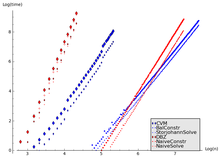
Figure 1: Timings for DBZ and CVM on input matrices $M$ of dimension $n$ and coefficients with fixed degree $d=15$ (smaller marks) or $d=20$ (larger marks)

We have implemented the DBZ algorithm and several variants of the CVM algorithm to evaluate the pertinence of our theoretical complexity analyses and the practical efficiency of our algorithmic improvements. Because of its fast implementations of polynomial and matrix multiplications, we chose the system Magma, using its release V2.16-7 on Intel Xeon 5160 processors (3 GHz) and 8 GB of RAM.

Our results are summarised in Table 1 and Figure 1. We fed our algorithms with matrices of size $n$ and coefficients of degree $d$ over $\mathbb{Z}/1048583\,\mathbb{Z}$. Linear regression on the logarithmic rescaling of the data was used to obtain parameters $c$, $e$, and $p$ that express the practical complexity of the algorithms in the form $cd^{e}n^{p}$. For the exponents $p$, both theoretical and experimental values are shown for comparison. Sample timings for particular $(n,d)$ are also given. BalConstr and NaiveConstr (resp. StorjohannSolve and NaiveSolve) compute the matrix $P$ (resp. $C$) of Algorithm 1 with or without the algorithmic improvements introduced in Theorem 8.

In Figure 1, each algorithm shows two parallel straight lines, for $d=15$ and 20, as was expected on a logarithmic scale. The improved algorithms are more efficient than their simpler counterparts when $n$ and $d$ are large enough.

The theory predicts $e=1$ for all algorithms. Observing different values suggests that too low values of $d$ have been used to reach the asymptotic regime. We also remark that, with respect to $d$, DBZ, BalConstr, and StorjohannSolve have slightly better practical complexity than their respective couterparts CVM, NaiveConstr, and NaiveSolve.

The practical exponent $p=3.00$ of BalConstr is smaller than $\theta+1$. The algorithm consists of $n$ executions of a loop that contains a constant number of scans of matrices and matrix multiplications. By analysing their contributions to the complexity separately, we obtain $2.5\ 10^{-6}d^{0.97}n^{3.00}$ for the former, and $5.2\ 10^{-8}d^{1.34}n^{3.19}$ for the latter. In the range of $n$ we are analysing, the first contribution dominates because of its constant, and its exponent $3.00$ is the only one visible on the experimental complexity of BalConstr.

It is also visible that StorjohannSolve is the dominating sub-algorithm of CVM. Besides, our implementation of StorjohannSolve is limited by memory and cannot handle matrices of dimension $n$ over 130. This bounds the size of the inputs manageable by our CVM implementation. A native Magma implementation of Storjohann’s algorithm should improve the situation. However, our implementation already beats the naive matrix inversion, so that the experimental exponent $3.88$ of StorjohannSolve is close to $\theta+1$.

The experimental exponent $p$ of DBZ is $6.01$ instead of $5$. This may be explained by the fact that the matrix coefficients that DBZ handles are fractions. Instead, in BalConstr, the coefficients are polynomial: denominators are extracted at the start of the algorithm and reintroduced at the end.

5 Conclusion

It would be interesting to study the relevance of uncoupling applied to system solving, and to compare this approach to direct methods. It would also be interesting to combine CVM and DBZ into a hybrid algorithm, merging speed of CVM and generality of DBZ.

References

- [1] S. Abramov and E. Zima. A universal program to uncouple linear systems. In Proceedings of CMCP’96, pages 16–26, 1997.
- [2] S. A. Abramov. EG-eliminations. J. Differ. Equations Appl., 5(4-5):393–433, 1999.
- [3] K. Adjamagbo. Sur l’effectivité du lemme du vecteur cyclique. C. R. Acad. Sci. Paris Sér. I Math., 306(13):543–546, 1988.
- [4] E. H. Bareiss. Sylvester’s identity and multistep integer-pre- serving Gaussian elimination. Math. Comp., 22:565–578, 1968.
- [5] M. A. Barkatou. An algorithm for computing a companion block diagonal form for a system of linear differential equations. Appl. Algebra Engrg. Comm. Comput., 4(3):185–195, 1993.
- [6] M. Bronstein and M. Petkovšek. An introduction to pseudo-linear algebra. Theor. Comput. Sci., 157(1):3–33, 1996.
- [7] D. G. Cantor and E. Kaltofen. On fast multiplication of polynomials over arbitrary algebras. Acta Inform., 28(7):693–701, 1991.
- [8] R. C. Churchill and J. Kovacic. Cyclic vectors. In Differential algebra and related topics, pages 191–218. 2002.
- [9] T. Cluzeau. Factorization of differential systems in characteristic . In Proc. ISSAC’03, pages 58–65. ACM, 2003.
- [10] F. T. Cope. Formal Solutions of Irregular Linear Differential Equations. Part II. Amer. J. Math., 58(1):130–140, 1936.
- [11] A. Dabèche. Formes canoniques rationnelles d’un système différentiel à point singulier irrégulier. In Équations différentielles et systèmes de Pfaff dans le champ complexe, volume 712 of Lecture Notes in Math., pages 20–32. 1979.
- [12] A. M. Danilevski. The numerical solution of the secular equation. Matem. sbornik, 44(2):169–171, 1937. (in Russian).
- [13] P. Deligne. Équations différentielles à points singuliers réguliers. Lecture Notes in Math., Vol. 163. Springer, 1970.
- [14] L. E. Dickson. Algebras and their arithmetics. Chicago, 1923.
- [15] B. Dwork and P. Robba. Effective -adic bounds for solutions of homogeneous linear differential equations. Trans. Amer. Math. Soc., 259(2):559–577, 1980.
- [16] S. Gerhold. Uncoupling systems of linear Ore operator equations. Master’s thesis, RISC, J. Kepler Univ. Linz, 2002.
- [17] M. Giesbrecht and A. Heinle. A polynomial-time algorithm for the Jacobson form of a matrix of Ore polynomials. In CASC’12, volume 7442 of LNCS, pages 117–128. Springer, 2012.
- [18] A. Hilali. Characterization of a linear differential system with a regular singularity. In Computer algebra, volume 162 of Lecture Notes in Comput. Sci., pages 68–77. Springer, 1983.
- [19] N. Jacobson. Pseudo-linear transformations. Ann. of Math. (2), 38(2):484–507, 1937.
- [20] A. Loewy. Über lineare homogene Differentialsysteme und ihre Sequenten. Sitzungsb. d. Heidelb. Akad. d. Wiss., Math.-naturw. Kl., 17:1–20, 1913.
- [21] A. Loewy. Über einen Fundamentalsatz für Matrizen oder lineare homogene Differentialsysteme. Sitzungsb. d. Heidelb. Akad. d. Wiss., Math.-naturw. Kl., 5:1–20, 1918.
- [22] L. Pech. Algorithmes pour la sommation et l’intégration symboliques. Master’s thesis, 2009.
- [23] E. G. C. Poole. Introduction to the theory of linear differential equations. Oxford Univ. Press, London, 1936.
- [24] L. Schlesinger. Vorlesungen über lineare Differentialgleichungen. B. G. Teubner, Leipzig, 1908.
- [25] A. Schönhage and V. Strassen. Schnelle Multiplikation großer Zahlen. Computing, 7:281–292, 1971.
- [26] A. Storjohann. High-order lifting and integrality certification. J. Symbolic Comput., 36(3-4):613–648, 2003.
- [27] V. Strassen. Gaussian elimination is not optimal. Numerische Mathematik, 13:354–356, 1969.
- [28] V. Vassilevska Williams. Multiplying matrices faster than Coppersmith-Winograd. In STOC’12, pages 887–898, 2012.
- [29] J. H. M. Wedderburn. Non-commutative domains of integrity. J. Reine Angew. Math., 167:129–141, 1932.
- [30] B. Zürcher. Rationale Normalformen von pseudo-linearen Abbildungen. Master’s thesis, ETH Zürich, 1994.