Energy exchange in Weyl geometry

Abstract

We study homogeneous and isotropic cosmologies in a Weyl spacetime. We show that the field equations can be reduced to the Einstein equations with a two-fluid source and analyze the qualitative, asymptotic behavior of the models. Assuming an interaction of the two fluids we impose conditions so that the solutions of the corresponding dynamical system remain in the physically acceptable phase space. We show that in Weyl integrable spacetime, the corresponding scalar field acts as a phantom field and therefore, it may give rise to a late accelerated expansion of the Universe.

1 Introduction

The usual approaches for an explanation of the late-time acceleration of the universe are characterized by a departure from conventional cosmology. The proposed models, either assume the existence of dark energy [1, 2], or require a modification of general relativity at cosmological distance scales [3, 4], (cf. [5, 6, 7, 8] for comprehensive reviews and references). Less explored is the idea that the geometry of spacetime is not the so far assumed Lorentz geometry (see for example [9]). Due to its simplicity Weyl geometry is considered as the most natural candidate for extending the Lorentzian structure.

We recall that a Weyl space is a manifold endowed with a metric $\mathbf{g}$ and a linear symmetric connection $\mathbf{\nabla}$ which are interrelated via

$$\nabla_{\mu}g_{\alpha\beta}=-Q_{\mu}g_{\alpha\beta},$$ (1)

where the 1-form $Q_{\mu}$ is customarily called Weyl covariant vector field (see the Appendix in [10] for a detailed exposition of the techniques involved in Weyl geometry). We denote by $D$ the Levi-Civita connection of the metric $g_{\alpha\beta}.$

A consistent way to incorporate an arbitrary connection into the dynamics of a gravity theory is the so-called constrained variational principle [11]. Applying this method in the context of Weyl geometry to the Lagrangian $L=R,$ one obtains the field equations

$$G_{\left(\mu\nu\right)}=-\nabla_{\left(\mu\right.}Q_{\left.\nu\right)}+Q_{\mu}Q_{\nu}+g_{\mu\nu}\left(\nabla^{\alpha}Q_{\alpha}-Q^{\alpha}Q_{\alpha}\right)=:M_{\mu\nu},$$

where $G_{\left(\mu\nu\right)}$ is the symmetric part of the Einstein tensor (see equations (30) and (31) in [11]). If we express the tensors $G_{\left(\mu\nu\right)}$ and $M_{\mu\nu}$ in terms of the quantities formed with the Levi-Civita connection $D$, the field equations become

$$\overset{\circ}{G}_{\mu\nu}=\frac{3}{2}\left(Q_{\mu}Q_{\nu}-\frac{1}{2}Q^{2}g_{\mu\nu}\right).$$ (2)

In the case of integrable Weyl geometry, i.e., when $Q_{\mu}=\partial_{\mu}\phi,$ the source term is that of a massless scalar field. Taking the divergence of (2) and using the Bianchi identities we conclude that

$$D^{\mu}Q_{\mu}=0.$$

In this paper we study Friedmann-Robertson-Walker (FRW) cosmologies in a Weyl framework. In Section 2 we explore the field equations derived from the Lagrangian $L=R+L_{m},$ where the matter Lagrangian, $L_{m},$ is chosen so that ordinary matter is described by a perfect fluid. It is shown that the presence of the Weyl vector field can be interpreted as a fluid and we analyze the asymptotic behavior of the models. Assuming an energy exchange between the two fluids we extend previous work [10]. In Section 3 we consider a modification of the Einstein-Hilbert Lagrangian, cf. (17), which may provide a mechanism of accelerating expansion.

2 Interacting fluids

In the following we assume an initially expanding FRW universe with expansion scale factor $a\left(t\right)$ and Hubble function $H=\dot{a}/a$. We adopt the metric and curvature conventions of [12]. An overdot denotes differentiation with respect to time $t,$ and units have been chosen so that $c=1=8\pi G.$ Ordinary matter is described by a perfect fluid with energy-momentum tensor,

$$T_{\mu\nu}=\left(\rho_{2}+p_{2}\right)u_{\mu}u_{\nu}+p_{2}g_{\mu\nu},$$ (3)

supplemented with an equation of state $p_{2}=\left(\gamma_{2}-1\right)\rho_{2}$. Since for spatially homogeneous and isotropic spacetimes there is no preferred direction, $Q^{\mu}$ must be proportional to the fluid velocity $u^{\mu}$, i.e.,

$$Q^{\mu}=:qu^{\mu},\;\;\;Q^{2}=Q_{\mu}Q^{\mu}=-q^{2}.$$

(In vacuum, we have to make the assumption that $Q^{\mu}$ is hypersurface orthogonal, i.e. it is proportional to the unit timelike vector field which is orthogonal to the homogeneous hypersurfaces). Formally the right-hand side of (2) can be rewritten as

$$\frac{3}{2}\left(Q_{\mu}Q_{\nu}-\frac{1}{2}Q^{2}g_{\mu\nu}\right)=\left(\rho_{1}+p_{1}\right)u_{\mu}u_{\nu}+p_{1}g_{\mu\nu},$$ (4)

with

$$\rho_{1}=p_{1}=\frac{3}{4}q^{2},$$ (5)

i.e., the equation of state of the $q-$fluid corresponds to stiff matter. Therefore we are dealing with a two-fluid model with total energy density and pressure given by

$$\rho=\rho_{1}+\rho_{2},\;\;\;p=p_{1}+p_{2},$$ (6)

respectively, where

$$p_{1}=\rho_{1},\;\;p_{2}=\left(\gamma_{2}-1\right)\rho_{2},$$ (7)

i.e., $\gamma_{1}=2$ and $\gamma_{2}<\gamma_{1}.$

The field equations are the Friedmann equation

$$H^{2}+\frac{k}{a^{2}}=\frac{1}{3}\left(\rho_{1}+\rho_{2}\right),$$ (8)

and the Raychaudhuri equation

$$\dot{H}=-H^{2}-\frac{1}{6}\left[\left(3\gamma_{1}-2\right)\rho_{1}+\left(3\gamma_{2}-2\right)\rho_{2}\right].$$ (9)

The Bianchi identities imply that the total energy-momentum tensor is conserved, so that an interaction between the two fluids is induced. It is necessary to make an assumption about the interaction between the two fluids (cf [13]), otherwise the field equations constitute an underdetermined system of differential equations. The simplest assumption is that the energy-momentum of each fluid is separately conserved, so that the two fluids do not interact and the densities decay independently,

$$\dot{\rho}_{1}=-3\gamma_{1}H\rho_{1},\ \ \ \ \dot{\rho}_{2}=-3\gamma_{2}H\rho_{2}.$$ (10)

The dynamical system (8)-(10) was analyzed in [10]. It was found that in expanding models the “real” fluid always dominates at late times and therefore the contribution of the Weyl fluid to the total energy-momentum tensor is important only at early times. The purpose of this section is to weaken the requirement of separate conservation of the two fluids.

In many cosmological situations the transfer of energy between two fluids is important, so one may assume that the two fluids exchange energy. The following simple model was proposed by Barrow and Clifton (see [14] for motivation and further examples),

$$\dot{\rho}_{1}=-3\gamma_{1}H\rho_{1}-\beta H\rho_{1}+\alpha H\rho_{2},$$ (11)

$$\dot{\rho}_{2}=-3\gamma_{2}H\rho_{2}+\beta H\rho_{1}-\alpha H\rho_{2},$$ (12)

where $\alpha$ and $\beta$ are constants so that the total energy is conserved (see also [15] for a singularity analysis of the master equation derived in [14]).

Remark 1

In the case of separately conserved fluids, equations (10) imply that the sets $\rho_{1}=0$ and $\rho_{2}=0,$ are invariant sets for the dynamical system and by standard arguments, if $\rho_{i}>0,\ i=1,2,$ for some initial time $t_{0}$, then $\rho_{i}(t)>0$ throughout the solution. This fact can be made more transparent by the following argument. Assuming that $\gamma_{1}>\gamma_{2},$ we define the transition variable $\chi\in[-1,1]$

$$\chi=\frac{\rho_{2}-\rho_{1}}{\rho_{2}+\rho_{1}},$$ (13)

which describes which fluid is dominant dynamically [13]. Applying the conservation equation to $\rho_{1}$ and $\rho_{2}$, one obtains the evolution equation of the variable $\chi$,

$$\dot{\chi}=\frac{3}{2}H\left(\gamma_{1}-\gamma_{2}\right)\left(1-\chi^{2}\right),$$ (14)

which implies that the sets $\chi=\pm 1$ are invariant under the flow of the dynamical system. Furthermore, the transition variable $\chi$ is bounded, that is, if initially $\chi\in[-1,1],$ it remains in that interval for all $t$. However, the choice (11) and (12), has the peculiarity that the sets $\rho_{1}=0$ and $\rho_{2}=0,$ are no longer invariant sets for the dynamical system and therefore the sign of the functions $\rho_{1}$ and $\rho_{2}$ is not conserved. This is also reflected to the fact that the transition variable $\chi$ no longer satisfies (14) and eventually escapes outside the interval $[-1,1]$, thus exhibiting unphysical behavior.

In order to circumvent these difficulties, one has to impose further conditions on $\alpha$ and $\beta$. It turns out that the assumption $\beta=-\alpha$ in (11) and (12) is a sufficient condition for the boundness of the function $\chi$. With this assumption we adopt the Coley and Wainwright formalism [13], for a general model with two fluids. The state of the system consists of the couple $\left(\chi,\Omega\right),$ where $\Omega=\Omega_{1}+\Omega_{2}$ is the total density parameter, $\Omega=\rho/3H^{2}.$ In order to allow for closed models in our analysis, we define the compactified density parameter $\omega,$ (see [16])

$$\Omega=\frac{1}{\tan^{2}\omega},$$ (15)

or

$$\omega=\arctan\left(\frac{\sqrt{3}H}{\sqrt{\rho}}\right),\,\;\;\;\text{with \ \ }-\pi/2\leq\omega\leq\pi/2.$$

We see that $\omega$ is bounded at the instant of maximum expansion ($H=0$) and also as $\rho\rightarrow 0,$ in ever-expanding models. Finally, defining a new time variable $\tau$ by

$$\frac{d\tau}{dt}=\frac{3\left(\gamma_{1}-\gamma_{2}\right)}{2}\sqrt{\frac{\rho}{3}}\frac{1}{\cos\omega},$$

one obtains the following dynamical system

$$\frac{d\omega}{d\tau} =-\frac{1}{2}\left(b-\chi\right)\cos 2\omega\cos\omega$$

$$\frac{d\chi}{d\tau} =(\chi_{\alpha}^{2}-\chi^{2})\sin\omega,$$ (16)

where the constant $b$ is

$$b=\frac{3\left(\gamma_{1}+\gamma_{2}\right)-4}{3\left(\gamma_{1}-\gamma_{2}\right)}>-1.$$

In our case, we always have $\gamma_{1}=2.$ The parameter $\chi_{\alpha}$ which determines the range of $\chi$ is given by

$$\chi_{\alpha}=\sqrt{1-\frac{4\alpha}{3\left(\gamma_{1}-\gamma_{2}\right)}},\ \ \ \ \ \ \ 0\leq\alpha\leq\frac{3\left(\gamma_{1}-\gamma_{2}\right)}{4}.$$

The phase space of the two-dimensional system (16) is the closed rectangle

$$D=\left[-\pi/2,\pi/2\right]\times\left[-\chi_{\alpha},\chi_{\alpha}\right]$$

in the $\omega-\chi$ plane (see Figure 1). Since $0\leq\chi_{\alpha}\leq 1,$ the rectangle $D$ is shrinked compared to the phase space in [10] and [16].

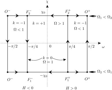
Figure 1: The invariant sets and equilibrium points of (16)

The invariant sets of the system are denoted in the following table.

$$\begin{array}[c]{lll}\omega=-\pi/2&\text{contracting empty models}&\Omega=0,H<0\\ \chi=-\chi_{\alpha}&\text{scaling solution}&\frac{\Omega_{2}}{\Omega_{1}}=\frac{1-\chi_{\alpha}}{1+\chi_{\alpha}}\\ \chi=+\chi_{\alpha}&\text{scaling solution}&\frac{\Omega_{1}}{\Omega_{2}}=\frac{1-\chi_{\alpha}}{1+\chi_{\alpha}}\\ \omega=\pi/4&\text{expanding flat models}&\Omega=1,H>0\\ \omega=-\pi/4&\text{contracting flat models}&\Omega=1,H<0\\ \omega=\pi/2&\text{expanding empty models}&\Omega=0,H>0\end{array}$$

It is easy to verify that the equilibrium points lie at the intersection of these sets and are denoted by $F_{1,2}^{\pm}$ (expanding or contracting flat model) and $O^{\pm}$ (expanding or contracting open model). The subscripts indicate which fluid dominates. Linearization around the equilibrium points is sufficient for the characterization of their stability and the result is the phase portrait is shown in Figure 2.

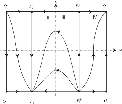
Figure 2: The phase portrait of (16) with $\gamma_{2}=1.$

Regions III and IV correspond to expanding models. The $F_{1}^{+}$ is a past attractor of all models with $\Omega>0$, i.e., the evolution near the big bang is approximated by the flat FRW model where the Weyl fluid dominates. Open models expand indefinitely and approach at late time a “scaling solution” where the Weyl fluid keeps a small fraction of the total energy density. Flat models expand indefinitely and the evolution is approximated by the flat FRW universe at late time. In both cases the “real” second fluid dominates at late times. On the other hand, any initially expanding closed model in region III, however close to $F_{2}^{+}$, eventually recollapses and the evolution is approximated by the flat FRW model where the Weyl fluid dominates.

We therefore conclude that the Weyl fluid has significant contribution only near the cosmological singularities. In expanding models the “real” fluid always dominates at late times and therefore the contribution of the Weyl fluid to the total energy-momentum tensor is important only at early times.

3 Phantom from pure geometry

The field equations (2) constitute the generalization of the Einstein equations in a Weyl spacetime in the sense that they come from the Lagrangian $L=R.$ There is however an alternative view, namely that the pair $\left(Q,\mathbf{g}\right)$ which defines the Weyl spacetime also enters into the gravitational theory and therefore, the field $Q$ must be contained in the Lagrangian independently from $\mathbf{g.}$ In the case of integrable Weyl geometry, i.e. when $Q_{\mu}=\partial_{\mu}\phi$ where $\phi$ is a scalar field, the pair $\left(\phi,g_{\mu\nu}\right)$ constitute the set of fundamental geometrical variables. We stress that the nature of the scalar field is purely geometric. A simple Lagrangian involving the set $\left(\phi,g_{\mu\nu}\right)$ is given by

$$L=R+\xi\nabla^{\mu}Q_{\mu}+L_{m},$$ (17)

where $\xi$ is a constant and $L_{m}$ corresponds to the Lagrangian yielding the energy-momentum tensor of a perfect fluid. Motivations for considering theory (17) can be found in [17, 18] (see also [19] for a multidimensional approach and [20] for an extension of (17) to include an exponential potential function of $\phi$). By varying the action corresponding to (17) with respect to both $g_{\mu\nu}$ and $\phi$ one obtains

$$\overset{\circ}{G}_{\mu\nu}=\frac{3-4\xi}{2}\left(\partial_{\mu}\phi\partial_{\nu}\phi-\frac{1}{2}\left(\partial_{\alpha}\phi\partial^{\alpha}\phi\right)g_{\mu\nu}\right)+T_{\mu\nu},$$ (18)

and

$$\overset{\circ}{\square}\phi=\frac{1}{3-4\xi}\rho,$$ (19)

where $\overset{\circ}{\square}$ is the D’Alembertian operator formed with the Levi-Civita connection $D$. As mentioned above, ordinary matter described by $T_{\mu\nu}$ is a perfect fluid with energy density $\rho$ and pressure $p$. Setting

$$\lambda=\frac{4\xi-3}{2},$$

we note that for $\lambda<0$ the field equations are formally equivalent to general relativity with a massless scalar field coupled to a perfect fluid. In Weyl spacetime the scalar field has a geometric nature and no restriction exists for the sign of the value of $\lambda$. For $\lambda>0,$ the Weyl field $\phi$ plays the role of a phantom scalar field and therefore, it may provide a mechanism of late time acceleration. Further investigation of this issue is the subject of future research.

References

- [1] Sahni S and Starobinsky A 2000 Int. J. Mod. Phys. D9 373
- [2] Peebles PJ and Ratra B 2003 Rev. Mod. Phys. 75 559
- [3] Carroll S, Duvvuri V, Trodden M and Turner M 2004 Phys. Rev. D70 043528
- [4] Chiba T 2003 Phys. Lett. B575 1
- [5] Copeland EJ , Sami M and Tsujikawa S 2006 Int. J. Mod. Phys. D15 1753
- [6] Sotiriou T and Faraoni V 2010 Rev. Mod. Phys. 82 451
- [7] De Felice A and Tsujikawa S 2010 Living Rev. Rel. 13 3
- [8] Bamba K, Capozziello S, Nojiri S, Odintsov SD 2012 Astrophysics and Space Science 342:155
- [9] Capozziello S, Carloni S and Troisi A 2003 Preprint astro-ph/0303041; Capozziello S, Cianci R, Stornaiolo C and Vignolo S 2008 Phys. Scripta 78:065010
- [10] Miritzis J 2004 Class. Quantum Grav. 21 3043
- [11] Cotsakis S, Miritzis J and Querella L 1999 J. Math. Phys. 40 3063
- [12] Wainwright J and Ellis GFR 1997 Dynamical Systems in Cosmology (Cambridge: Cambridge University Press)
- [13] Coley AA and Wainwright J 1992 Class. Quantum Grav. 9 651
- [14] Barrow JD and Clifton T 2006 Phys. Rev. D73 103520
- [15] Cotsakis S and Kittou G 2012 Phys. Lett. B712 16
- [16] Wainwright J 1996 Relativistic Cosmology In Proceedings of the 46th Scottish Universities Summer School in Physics Aberdeen pp 107-141 Eds GS Hall and JR Pulham (Institute of Physics Publishing)
- [17] Novello M, Oliveira LAR, Salim JM and Elbas E 1993 Int. J. Mod. Phys. D1 N 3-4 641
- [18] Salim JM and Sautu SL 1996 Class. Quantum Grav. 13 353
- [19] Konstantinov MY and Melnikov VN 1995 Int. J. Mod. Phys. D4 339
- [20] Oliveira HP, Salim JM and Sautu SL 1997 Class. Quantum Grav. 14 2833