Exploring Quantum Contextuality to Generate True Random Numbers

Abstract

Random numbers represent an indispensable resource for many applications. A recent remarkable result is the realization that non-locality in quantum mechanics can be used to certify genuine randomness through Bell’s theorem, producing reliable random numbers in a device independent way. Here, we explore the contextuality aspect of quantum mechanics and show that true random numbers can be generated using only single qutrit (three-state systems) without entanglement and non-locality. In particular, we show that any observed violation of the Klyachko-Can-Binicioglu-Shumovsky (KCBS) inequality [Phys. Rev. Lett. 101, 20403 (2008)] provides a positive lower bound on genuine randomness. As a proof-of-concept experiment, we demonstrate with photonic qutrits that at least $5246$ net true random numbers are generated with a confidence level of $99.9\%$.

Random numbers are widely used in algorithms and technology 1982Yao ; 1981Knuth . However, generation of genuine randomness is a challenging task 2010Pironio . Mathematically, randomness means unpredictability 2011Abbott ; Chaitin-Book . Thus, in principle, random numbers can never be generated by a classical device since any classical system bears a deterministic description. Consequently, random numbers generated by a classical device can always be attributed to a lack of knowledge about the device. If we know all the information of the device, in principle we can predict all the results of any operation on this device. Unlike classic systems, quantum theory is intrinsically random. It is natural to think about generating random numbers via a quantum device. In fact, various quantum random number generators (QRNGs) have already been reported. Significant examples include those based on the decay of radioactive nucleus 1956Isida , beam splitters 1990Svozil ; 1994Rarity ; 2000Jennewein , entangled photon pairs 2004Ma and amplified quantum vacuum 2011Jofre . However, in real experiment the intrinsic randomness of these QRNGs is inevitably mixed-up with an apparent randomness due to noise or lack of control of the experiment. In other words, the randomness generated by these QRNGs cannot be unequivocally certified or quantified. This will jeopardize some applications of randomness, especially cryptographic applications. A breakthrough was made by Colbeck 2007Colbeck and subsequently developed by Pironio et al 2010Pironio ; correction . The basic idea is to use the non-local correlation of quantum states to generate certified private randomness. More specifically, Bell’s theorem can be used to certify genuine randomness. In Ref. 2010Pironio , taking the Clauser-Horn-Shimony-Holt (CHSH) inequality 1969Clauser as an example, Pironio et al demonstrated for the first time this important idea with a proof-of-concept experiment using entangled trapped ions. A more recent work in this direction is Ref. 2012VV .

Here, we introduce a new method to generate true random numbers in single-qutrit systems through exploration of the Kochen-Specker (KS) theorem. Generation of randomness by this method does not rely on the costly quantum resource of entanglement, which significantly simplifies its experimental realization. The Kochen-Specker theorem 1960Specker ; 1966Bell ; 1967Kochen states that no non-contextual hidden variable model (NCHVM) can reproduce the prediction of quantum mechanics, or simply put, quantum mechanics is contextual. In recent years, extensive works on quantum contextuality have been done, including both theoretical analyses 2008KCBS ; 1990Peres ; 1990Mermin ; 2008Cabello ; 2012Yu and experiment demonstrations 2000Michler ; 2009Kirchmair ; 2009Bartosik ; 2009Amselem ; 2010Moussa ; 2011Lapkiewicz ; 2012Zu . All the experimental results favor quantum mechanics and hence rule out the NCHVM. Here, we exploit this theorem from a new angle and show that it can be used to generate genuine randomness. To this end, we explore a KS inequality introduced recently by Klyachko, Can, Binicioglu and Shumovsky (KCBS) 2008KCBS , and show that any observed violation of the KCBS inequality leads to a positive lower bound on the randomness produced by the quantum device. Furthermore, as a proof-of-concept experiment, we demonstrate this new method with photonic qutrits by showing that at least $5246$ net true random numbers are generated with a confidence level of $99.9\%$.

To be specific, we consider a single qutrit system and five two-outcome measurements $A_{i}$ $(i=1,2,3,4,5)$. Denoting the outcome of the the corresponding measurement $A_{i}$ as $a_{i}$ ($a_{i}=0,1$), the KCBS inequality can be rewritten as 2008KCBS ; 2011Lapkiewicz :

$$L\equiv\sum_{(i,j)\in\mathcal{S}}[P(a_{i}\neq a_{j}|A_{i}A_{j})-P(a_{i}=a_{j}|A_{i}A_{j})]\leq 3,$$ (1)

where $\mathcal{S}=\{(1,2),(2,3),(3,4),(4,5),(5,1)\}$ represents the set of pairs of compatible (commutable) measurements, and $P(a_{i}\neq a_{j}|A_{i}A_{j})$ ($P(a_{i}=a_{j}|A_{i}A_{j})$) is respectively the probability that $a_{i}\neq a_{j}$ ($a_{i}=a_{j}$) when the measurement setting $(A_{i},A_{j})$ is chosen. The inequality (7) is satisfied by any NCHVM. In quantum mechanics, however, this inequality can be violated for certain measurements performed on a specific state and the maximal violation is $4\sqrt{5}-5\approx 3.944$ 2008KCBS . An experimental violation has been reported recently in Ref. 2011Lapkiewicz . For our purpose to relate the KCBS violation to the generation of randomness, we run the experiment $k$ times in succession. The measurement choice $(A_{i},A_{j})$ for each trial is generated by a computer through an identical and independent probability distribution $P(A_{i}A_{j})$ ($(i,j)\in\mathcal{S}$). Denoting the input string as $\mathcal{I}=(A_{i_{1}},A_{j_{1}};\cdots;A_{i_{k}},A_{j_{k}})$ and the corresponding output string as $\mathcal{O}=(a_{i_{1}},a_{j_{1}};\cdots;a_{i_{k}},a_{j_{k}})$, the estimated KCBS violation can be obtained from the observed data as

$$\hat{L}=\frac{1}{k}\sum_{(i,j)\in\mathcal{S}}[N(a_{i}\neq a_{j}|A_{i}A_{j})-N(a_{i}=a_{j}|A_{i}A_{j})]/P(A_{i}A_{j}),$$ (2)

where $N(a_{i}\neq a_{j}|A_{i}A_{j})$ ($N(a_{i}=a_{j}|A_{i}A_{j})$) denotes respectively the number of trials with unequal (equal) measurement outcomes under the measurement setting $(A_{i},A_{j})$.

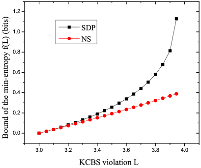
Figure 1: The min-entropy bound $f(L)$ versus different levels $L$ of the KCBS violation. The black-square line is obtained through optimization based on the semi-definite programming (SDP) assuming validity of quantum mechanics. We can relax this assumption and do not assume the formalism of quantum mechanics, but only require that for two compatible (commutable) observables, a measurement on one observable does not change the marginal probability distribution of measurement outcomes of the other observable. This corresponds to the no signaling (NS) condition for bi-partite system and we still call it the NS condition. The red-dotted line corresponds to an analytical lower-bound $f(L)=-\log_{2}(1.75-L/4)$ obtained under the NS condition only (see the supporting information for a detailed derivation).

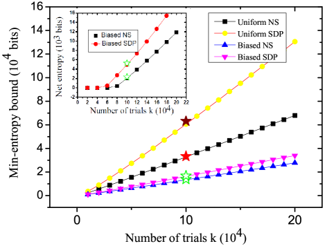
Figure 2: The min-entropy bound $kf(\mathcal{L}_{m}-\epsilon)-\log_{2}\frac{1}{\delta}$ versus the number of trials $k$ assuming that the observed KCBS violation lies within the interval $3.9=\mathcal{L}_{m}\leq\hat{L}<\mathcal{L}_{m+1}=4\sqrt{5}-5\approx 3.944$ with non-negligible probability $\delta$. Here the parameters are chosen as $\delta=0.001$ and $\epsilon^{\prime}=0.01$. We take two different distributions for the input pairs $(A_{i},A_{j})$: a uniform distribution with $P(A_{i}A_{j})=1/5$ $(i,j)\in\mathcal{S}$, and a biased distribution with $P(A_{1}A_{2})=1-4\alpha k^{-1/2}$, $P(A_{2}A_{3})=P(A_{3}A_{4})=P(A_{4}A_{5})=P(A_{1}A_{5})=\alpha k^{-1/2}$, and $\alpha=6$. According to Table I, the KCBS violations for the uniform and biased cases are $\hat{L}^{uni}=3.924$ and $\hat{L}^{bia}=3.905$, respectively. Thus, both $\hat{L}^{uni}$ and $\hat{L}^{bia}$ lie within the interval $[3.9,3.944)$. We plot both min-entropy bounds $kf(\mathcal{L}_{m}-\epsilon)-\log_{2}\frac{1}{\delta}$ based respectively on the SDP optimization and the NS condition (see caption of Fig. 1). The stars represent the experimental data where approximately $10^{5}$ measurement outcomes are recorded from the detectors ($k\approx 10^{5}$). The inset shows the lower bounds of the net entropy (the output entropy minus the input entropy for distribution $P(A_{i}A_{j})$) for the biased cases. We get about $5246$ net random numbers from the experimental data for the biased SDP case.

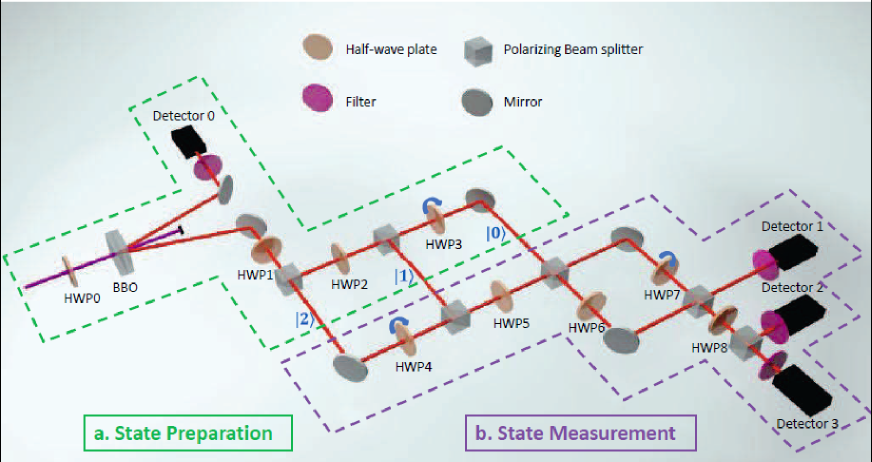
Figure 3: Schematic experimental setup of a ture quantum random number generator. (a) State preparation of a single photonic qutrit. Ultrafast laser pulses (with a repetition rate of $76$ MHz) at the wavelength of $400$ nm from a frequency doubled Ti:sapphire laser pump two joint beta-barium-borate (BBO) crystals and generate correlated photon pairs at the wavelength of $800$ nm. A photon-count at the detector D$0$ heralds a single photon at the other output port, which is split by two polarizing beam splitters (PBS) into three spatial models, representing a single photonic qutrit. By adjusting the orientations of the half wave plates (HWP1 and HWP2), we can prepare any qutrit state. The setup in box (b) implements the measurements. By tuning the wave plates (HWP5, HWP6, and HWP8), we measure the probability $P(a_{i}a_{j}|A_{i}A_{j})$ for a pair of compatible observables $(A_{i},A_{j})$ $(i,j)\in\mathcal{S}$. The input pairs $(A_{i},A_{j})$ are chosen according to the distribution $P(A_{i}A_{j})$. To get the desired $(A_{i},A_{j})$, the orientations of HWPs are listed in the Supporting information. The wave plates HWP3, HWP4, and HWP7 can be tilted to balance the Mach-Zender interferometers and their angle are set to zero. The photons are recorded by single photon detectors D0-D3 after spectra-filters of $3$ nm bandwidth for coincidence measurements.

Let $\{\mathcal{L}_{m}:0\leq m\leq m_{max}\}$ be a series of KCBS violation thresholds with $\mathcal{L}_{0}=3$ and $\mathcal{L}_{m_{max}}=4\sqrt{5}-5$ corresponding respectively to the classical and quantum bound, and denote $\mathcal{D}(m)$ the probability that the observed KCBS violation $\hat{L}$ lies in the interval $[\mathcal{L}_{m},\mathcal{L}_{m+1})$, then we can use the min-entropy to quantify randomness of the output string $\mathcal{O}$ 2010Pironio ; 2012Pironio ; 2009Koenig :

$$E_{\infty}(\mathcal{O}|\mathcal{I},\mathcal{E},m)_{\mathcal{D}}\equiv-\mathtt{log}_{2}\sum_{\mathcal{I},\mathcal{E}}\mathcal{D}(\mathcal{I},\mathcal{E}|m)[\max_{\mathcal{O}}\mathcal{D}(\mathcal{O}|\mathcal{I},\mathcal{E},m)],$$ (3)

where $\mathcal{E}$ represents the knowledge that a possible adversary has on the state of the device and the maximum is taken over all possible values of the output string $\mathcal{O}$; the probability distribution $\mathcal{D}(\mathcal{O},\mathcal{I},\mathcal{E})$ is defined in the supplementary information. In order to build a link between the KCBS violation and randomness, we assume: (i) the system can be described by quantum theory; (ii) the input $(A_{i_{l}},A_{j_{l}})$ is chosen at step $l$ from an independent random distribution uncorrelated with the system; (iii) the pair of measurements at step $l$ are compatible (one measurement does not influence the marginal distribution of the outcomes of the other measurement); (iv) the adversary’s side-information is classical. Based on these assumptions, we can show that if $\mathcal{D}(m)>\delta$, the min-entropy of the output string conditioned on the input string and the adversary’s information has a lower bound (see derivation in Sec. II of the supplementary information):

$$E_{\infty}(\mathcal{O}|\mathcal{I},\mathcal{E},m)_{\mathcal{D}}\geq kf(\mathcal{L}_{m}-\epsilon)-\log_{2}\frac{1}{\delta},$$ (4)

where the parameter $\epsilon\equiv\{-2[1+(4\sqrt{5}-5)r]^{2}(\ln\epsilon^{\prime})/(kr^{2})\}^{\frac{1}{2}}$ with $r=\min P(A_{i}A_{j})$, the smallest probability of the input pairs; $\epsilon^{\prime}$ is another given parameter denoting the closeness between the resulting distribution that characterize $k$ successive use of the device and another extended distribution that is well defined mathematically. The function $f(L)$ is obtained by semi-definite programming (SDP) 1996Vandenberghe and is shown in Fig. 1; and the min-entropy bound $kf(\mathcal{L}_{m}-\epsilon)-\log_{2}\frac{1}{\delta}$ for different numbers of trials $k$ is plotted in Fig. 2. It is remarkable that other than the above four basic assumptions, there is no further constraint on the states, measurements, or the Hilbert space. It also requires no assumption that the system behaves identically and independently for each trial. In particular, the system may have an internal memory (classical or quantum) so that the results of the $l$th trial depend on the previous $l-1$ trials. Any observed violation of the KCBS inequality with $\hat{L}>3$ leads to a positive lower bound on the min-entropy, and thus guarantees genuine randomness generated by the quantum device.

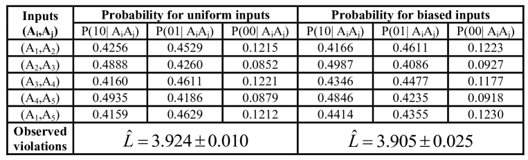
Figure 4: Table I: Experimentally observed probabilities and the corresponding KCBS violation under uniform or biased distribution $P(A_{i}A_{j})$ (see caption of Fig. 2 for specification). The probability $P(11|A_{i}A_{j})$ is negligible as the three-photon coincidence rate is typically smaller than the two-photon coincidence rate between D0 and Di by more than four orders of magnitude and thus much less than the error bar. For both cases, the KCBS inequality is significantly violated, guaranteeing the generation of genuine randomness.

In order to experimentally implement our scheme, we use photonic qutrits where the states are represented by three different paths of a single photon. For each photonic qutrit, we randomly choose the compatible measurement configurations $(A_{i}A_{j})$ from the set $\mathcal{S}$ according to a certain probability distribution $P(A_{i}A_{j})$ (uniform or biased, with its form given in caption of Fig. 2) and record the measurement outcomes $(a_{i},a_{j})$, which gives our output random bits. To generate random numbers, we need to observe violation of the KCBS inequality and the level of violation gives bound on genuine randomness according to Eq. (4). Different from the experiment in Ref. 2011Lapkiewicz on test of quantum contextuality with the KCBS inequality, to generate randomness, the input pairs $(A_{i},A_{j})$ need to be chosen randomly according to a probability distribution $P(A_{i}A_{j})$ (instead of fixed before the experiment), and we need to record the whole measurement output sequence $\mathcal{O}=(a_{i_{1}},a_{j_{1}};\cdots;a_{i_{k}},a_{j_{k}})$ instead of simply the total number of events $N(a_{i}\neq a_{j}|A_{i}A_{j})$ and $N(a_{i}=a_{j}|A_{i}A_{j})$).

The experimental setup is depicted in Fig. 3. The spontaneous parametric down conversion (SPDC) process generates entangled photon pairs. Through detection of one of the photons by a detector D0, we get a heralded single-photon source on the other output mode. Two polarization beam splitters (PBS) split this heralded photon into three spatial models, representing a single photonic qutrit. Any state of this photonic qutrit can be prepared by adjusting the orientations of the wave plates before the PBS. The measurements are implemented by three half wave plates and three single-photon detectors D1-D3. The angles of these wave plates corresponding to different pairs of compatible observables are listed in the supporting information (Table 1 of Sec. IV). We assign value $1$ ($0$) to the observable $A_{i}$ under a click (non-click) of the corresponding detector. Due to the inevitable photon loss, there could be no click on the detectors D1-D3 even when the detector D0 records an event. We discard all the events in which only the trigger detector D0 and none of the measurement detectors D1-D3 fires. This is the post-selection technique commonly used in the photon experiments 2011Lapkiewicz , which opens up the detection efficiency loophole. We thus need the fair-sampling assumption that the photons selected out by the coincidence measurement represent a fair sampling of all the events. The detection efficiency loophole can be closed by using single-ion qutrits, where one can follow the same experimental procedure here and generate true random numbers using only high-speed single-bit rotations.

The experimental results are summarized in Table I. For both the uniform and biased input cases, we record about $k\approx 10^{5}$ events. The observed KCBS violation indicates that $E_{\infty}^{\mathtt{uni}}(\mathcal{O}|\mathcal{I},\mathcal{E},m)>6.3\times 10^{4}$ and $E_{\infty}^{\mathtt{bia}}(\mathcal{O}|\mathcal{I})>1.6\times 10^{4}$ with a $99.9\%$ confidence level, so tens of thousands of genuine random numbers have been generated in both cases. Similar to Ref. 2010Pironio , the scheme described here is actually a randomness expansion scheme, where a larger random string (the measurement outcome $\mathcal{O}$) is generated from a smaller set of random seed which serves as the input $\mathcal{I}$ to specify the measurement configuration $(A_{i}A_{j})$. A figure of merit for the randomness expansion scheme is the net rate of random bits, defined as the number of bits generated minus the number of bits consumed. In the entanglement based experiment 2010Pironio , it is still difficult to get a positive net rate of random bits with the current technology because of the slow entanglement generation rate. In our experiment, for the biased case, we have achieved a positive net rate for the first time with the output entropy exceeding the input entropy, leading to approximately $5246$ net random bits. We have performed extensive random tests on the output strings in our experiment. The results are summarized in the supplementary information.

We have proposed a scheme to generate genuine random numbers in qutrit systems where the randomness is guaranteed by violation of the KCBS inequality, a version of the Kocher-Specker theorem resulting from quantum contextuality. This scheme guarantees randomness without the need of using costly quantum resource such as entanglement, and allows for easier implementation and significantly higher generation rate of random strings. We have demonstrated this scheme with a proof-of-concept experiment using photonic qutrits and achieved for the first time a positive net rate of ture random numbers. The scheme can be readily implemented with other experimental systems, such as single trapped ions, to close the detection loophole, opening up practical prospect to generate ture random numbers with high speeds.

This work was supported by the NBRPC (973 Program) 2011CBA00300 (2011CBA00302) and the NSFC Grant 61033001. DLD and LMD acknowledge in addition support from the IARPA MUSIQC program, the ARO and the AFOSR MURI program.

Note added.—-Having finished this work, we became aware of a recent theoretical work 2012Abbott , which explored the Kochen-Specker theorem in another different way to generate randomness.

I Supplementary information: Exploring Quantum Contextuality to Generate True Random Numbers

In this supporting information, we give a detailed derivation of the link between generation of randomness and violation of the Klyachko-Can-Binicioglu-Shumovsky (KCBS) inequality. For completeness, we also briefly explain the specific KCBS inequality used in our experiment. On the experimental side, we give detailed configurations of the wave plates in our experiment and present results for several random tests on the output data string from the experimental measurements.

I.1 I. The KCBS inequality

The KCBS inequality was first introduced in Ref. 2008KCBS . It corresponds to a state-dependent proof of the Kochen-Specker theorem for a qutrit system. For completeness, here we give a brief derivation. Consider five two-outcome observables $A_{i}$ $(i=1,2,3,4,5)$ and denote their outcomes as $a_{i}$, whose values are assigned to be $-1$ or $+1$ (one can also denote the two outcomes as $0$ and $1$ as in the main text). For any such assignments, the following algebraic inequality holds:

$$-a_{1}a_{2}-a_{2}a_{3}-a_{3}a_{4}-a_{4}a_{5}-a_{5}a_{1}\leq 3.$$ (5)

To arrive at the above inequality, we note that the product of the five monomials on the left-hand side is $-1$. Consequently, at least one term is equal to $-1$, and the sum of the remaining four terms should not exceed $4$. We thus get the above inequality. According to the non-contextual hidden variable model (NCHVM), if the outcomes $a_{i}$ are described by an unknown probability distribution, we can integrate over the distribution to take average and the expectation values of the corresponding observables $A_{i}$ then satisfy

$$-\langle A_{1}A_{2}\rangle-\langle A_{2}A_{3}\rangle-\langle A_{3}A_{4}\rangle-\langle A_{4}A_{5}\rangle-\langle A_{5}A_{1}\rangle\leq 3,$$ (6)

Note that $\langle A_{i}A_{j}\rangle=P(a_{i}=a_{j}|A_{i}A_{j})-P(a_{i}\neq a_{j}|A_{i}A_{j})$, so the above inequality (6) can also be written into the following form as shown in the main text:

$$L\equiv\sum_{(i,j)\in\mathcal{S}}[P(a_{i}\neq a_{j}|A_{i}A_{j})-P(a_{i}=a_{j}|A_{i}A_{j})]\leq 3.$$ (7)

Any NCHVM should obey the inequality (7). However, quantum mechanics violates this inequality for certain measurements on a specific state. In our experiment, we choose the state to be $\left|\Phi_{0}\right\rangle=|0\rangle$. The five observables are chosen as $A_{i}=2|\psi_{i}\rangle\langle\psi_{i}|-\mathbf{I}=2(\alpha_{i}|0\rangle+\beta_{i}|1\rangle+\gamma_{i}|2\rangle)(\alpha_{i}\langle 0|+\beta_{i}\langle 1|+\gamma_{i}\langle 2|)-\mathbf{I}$, where $\mathbf{I}$ is the $3\times 3$ identity matrix and $\alpha_{1}=\alpha_{2}=\alpha_{3}=\alpha_{4}=\alpha_{5}=\sqrt{\sqrt{5}/5}$, $\beta_{1}=-\frac{\sqrt{2}}{2}\cos^{-1}\frac{\pi}{10}$, $\beta_{3}=\beta_{4}=-\frac{\sqrt{2}}{2}\tan\frac{\pi}{10}$, $\beta_{2}=\beta_{5}=-\beta_{1}\cos\frac{\pi}{5}$, $\gamma_{1}=0$, $\gamma_{2}=-\gamma_{5}=\beta_{1}\sin\frac{\pi}{5}$, and $\gamma_{4}=-\gamma_{3}=-\sqrt{2}/2$. One can check that all the pairs $(A_{i},A_{j})$ with $(i,j)\in\mathcal{S}$ are compatible (i.e., $A_{i}$ and $A_{j}$ commute). It is straightforward to show that for these specific measurements $A_{i}$ under the state $\left|\Phi_{0}\right\rangle$, quantum mechanics predicts that $L=4\sqrt{5}-5\approx 3.944>3$, thus violates the KCBS inequality (7) imposed by any NCHVM.

I.2 II. Generation of randomness via violation of the KCBS inequality

To establish a link between quantum contextuality and randomness, we use notations and arguments similar to Ref. 2010Pironio ; 2012Pironio for the Bell’s inequality case correction . We say that the observables $O=\{O_{A_{i}}^{a_{i}}\}$ $(i=1,2,3,4,5)$ and the state $\rho$ give a quantum realization of the joint probability $P_{\mathbf{a}_{i}\mathbf{a}_{j}|\mathbf{A}_{i}\mathbf{A}_{j}}=\{P(a_{i}a_{j}|A_{i}A_{j})\}$ if $P(a_{i}a_{j}|A_{i}A_{j})=\mathtt{Tr}(\rho O_{A_{i}}^{a_{i}}O_{A_{j}}^{a_{j}})$. Here, $O_{A_{i}}^{a_{i}}$ is a projector that projects the state onto an eigenstate of the observable $A_{i}$ with eigenvalue $a_{i}$. For simplicity, we denote the quantum realization and the joint probability distribution as a triplet $\{\rho,O,P\}$. For one trial of experiment, the randomness of the output pairs conditioned on the input pairs $(A_{i},A_{j})$ is defined as the min-entropy:

$$E_{\infty}(\mathbf{a}_{i}\mathbf{a}_{j}|\mathbf{A}_{i}\mathbf{A}_{j})=-\log_{2}[\max_{a_{i}a_{j}}P(a_{i}a_{j}|A_{i}A_{j})]$$ (8)

For any quantum realization of the joint probability $P_{\mathbf{a}_{i}\mathbf{a}_{j}|\mathbf{A}_{i}\mathbf{A}_{j}}$ and a given KCBS violation $L$, we aim to find a lower bound on the min-entropy:

$$E_{\infty}(\mathbf{a}_{i}\mathbf{a}_{j}|\mathbf{A}_{i}\mathbf{A}_{j})\geq f(L).$$ (9)

This is equivalent to solution of the following optimization problem:

$$\max \quad\quad\quad P(a_{i}a_{j}|A_{i}A_{j})$$ (10)

$$\mathtt{subject}\text{ }\mathtt{to} \sum_{(i,j)\in\mathcal{S}}[P(a_{i}\neq a_{j}|A_{i}A_{j})-P(a_{i}=a_{j}|A_{i}A_{j})]=L$$

$$P(a_{i}a_{j}|A_{i}A_{j})=\mathtt{Tr}(\rho O_{A_{i}}^{a_{i}}O_{A_{j}}^{a_{j}})$$

where the optimization is carried over all quantum realizations $\{\rho,O,P\}$. Denote by $P^{\ast}(a_{i}a_{j}|A_{i}A_{j})$ the solution to the above problem, then the minimal value of $E_{\infty}(\mathbf{a}_{i}\mathbf{a}_{j}|\mathbf{A}_{i}\mathbf{A}_{j})$ consistent with the quantum theory and the KCBS violation $L$ is given by $E_{\infty}(\mathbf{a}_{i}\mathbf{a}_{j}|\mathbf{A}_{i}\mathbf{A}_{j})=-\log_{2}P^{\ast}(a_{i}a_{j}|A_{i}A_{j})$. To get a bound independent of the input pair $(A_{i},A_{j})$, we should further minimize $E_{\infty}(\mathbf{a}_{i}\mathbf{a}_{j}|\mathbf{A}_{i}\mathbf{A}_{j})$ over all the input pairs $(A_{i},A_{j})$. This leads to a lower bound $f(L)$ on the min-entropy determined by the KCBS violation $L$ only.

The above optimization problem can be efficiently solved by casting it to a semi-definite programing (SDP) problem. In Refs. 2007Navascues ; 2008Navascues , an infinite hierarchy of conditions satisfied by all quantum correlations are introduced, and the hierarchy is complete in the asymptotic limit, i.e., if all the conditions in the hierarchy are satisfied, there always exists a quantum realization $\{\rho,O,P\}$. All the conditions in the hierarchy can be transformed to a SDP problem. In general, conditions higher in the hierarchy are more constraining and thus give a tighter lower bound $f(L)$ to $E_{\infty}(\mathbf{a}_{i}\mathbf{a}_{j}|\mathbf{A}_{i}\mathbf{A}_{j})$. We use the matlab toolboxes SeDuMi Sturm-Sedumi to solve the SDP problem for the optimization. The result is plotted in Fig. 1 of the main text. From the figure, $f(L)$ equals zero at the classical boundary $L=3$ and increases monotonously as the KCBS violation $L$ increases. For the maximal violation $L=4\sqrt{5}-5$, $P^{\ast}=0.457$, corresponding to $f(L)\simeq 1.13$ bits.

We can obtain an upper bound on the min-entropy by numerically searching for solutions to Eq. (10) under a fixed dimension of the Hilbert space. When the Hilbert space dimension is fixed to be $3,$ we find that the upper bound coincides with the lower bound up to a precision of $10^{-5}$. This indicates that the lower bound obtained above is tight.

The above bound depends on the quantum violation $L$ of the KCBS inequality, which itself needs to be determined from a finite runs of experiments. Now we derive a practical bound on the min-entropy that can be determined from a finite runs of experiments, taking into account the statistical error on estimation of the quantum violation $L$ and the classical side information a possible adversary may have on the device. To this end, let’s first introduce the following theorem:

Theorem 1. Suppose we run the experiments $k$ times and the sequence of inputs $\mathcal{I}=(A_{i_{1}},A_{j_{1}};\cdots;A_{i_{k}},A_{j_{k}})$ is generated by choosing each pair of inputs $(A_{i_{n}},A_{j_{n}})$ independently with probability $P(A_{i}A_{j})$. Let $\delta$, $\epsilon^{\prime}>0$ be two arbitrary parameters and $r=\min_{ij}\{P(A_{i}A_{j})\}$, then the distribution $P(\mathcal{O}\mathcal{I}\mathcal{E})$ characterizing $k$ successive use of the devices is $\epsilon^{\prime}$-close to a distribution $\mathcal{D}$ such that, either $\mathcal{D}(m)\leq\delta$ or

$$E_{\infty}(\mathcal{O}|\mathcal{I},\mathcal{E},m)_{\mathcal{D}}\geq kf(\mathcal{L}_{m}-\epsilon)+\log_{2}\delta,$$ (11)

where $\epsilon=(L_{q}+1/r)\sqrt{-2\ln\epsilon^{\prime}/k}$ with $L_{q}=4\sqrt{5}-5$ denoting the maximal KCBS violation.

Proof. We follow similar procedures and arguments in Ref. 2012Pironio to prove the above theorem. Define a function $\mathcal{F}(L)=2^{-f(L)}$, then from the solutions to the optimization problem Eq. 10 and Fig. 2 in the main text, it is easy to obtain that $\mathcal{F}$ is a concave and monotocially decreasing function. Denote by $\mathcal{O}^{n}=(a_{i_{1}},a_{j_{1}};\cdots;a_{i_{n}},a_{j_{n}})$ ($n\leq k$) the string of outputs before the $(n+1)$th round of experiment (similarly, $\mathcal{I}^{n}$ denotes the string of inputs). We define an indicator function $\chi(e)$ as: $\chi(e)=1$ if the event $e$ happens and $\chi(e)=0$ otherwise. Consider the following random variable

$$\hat{L}_{l}=\sum_{(\mu\nu);(x,y)\in\mathcal{S}}\tau(\mu,\nu)\frac{\chi(a_{i_{l}}=\mu,a_{j_{l}}=\nu;A_{i_{l}}=x,A_{j_{l}}=y)}{P(xy)},$$ (12)

where $\mathcal{S}$ is defined in the main text and $\tau(\mu,\nu)$ $(\mu,\nu=0,1)$ is a sign function defined as: $\tau(\mu,\nu)=-1$ if $\mu=\nu$ and $\tau(\mu,\nu)=1$ otherwise. It is straightforward to see that Eq. (12) corresponds to the KCBS expression (2) in the main text and the expectation value of $\hat{L}_{l}$ conditional on $W^{l}$ is equal to $L(W^{l})$, i.e., $\mathbb{E}(\hat{L}|W^{l})=L(W^{l})$. Here $\mathcal{W}^{l}\equiv(\mathcal{O}^{l-1}\mathcal{I}^{l-1}\mathcal{E})$ denotes all the events before the $l$th round of experiment and the possible adversary’s classical side information. Let $\hat{L}=\frac{1}{k}\sum_{l=1}^{k}\hat{L}_{l}$ be our estimator of the KCBS violation. After specify the above notations, now let’s also introduce two lemmas for the proof of the theorem:

Lemma 1. For a given parameter $\epsilon^{\prime}>0$, let $\epsilon=(L_{q}+1/r)\sqrt{-2\ln\epsilon^{\prime}/k}$ and $\mathcal{T}_{\epsilon}=\{(\mathcal{O},\mathcal{I},\mathcal{E})|\frac{1}{k}\sum_{l=1}^{k}\mathbb{E}(\hat{L}_{l}|W^{l})\geq\hat{L}(\mathcal{O},\mathcal{I})-\epsilon\}$, then we have:

(i) for any $(\mathcal{O},\mathcal{I},\mathcal{E})\in\mathcal{T}_{\epsilon}$,

$$P(\mathcal{O}|\mathcal{I}\mathcal{E})\leq\mathcal{F}^{k}(\hat{L}(\mathcal{O},\mathcal{I})-\epsilon).$$ (13)

(ii)

$$\texttt{Pr}(\mathcal{T}_{\epsilon})=\sum_{(\mathcal{O},\mathcal{I},\mathcal{E})\in\mathcal{T}_{\epsilon}}P(\mathcal{O},\mathcal{I},\mathcal{E})\geq 1-\epsilon^{\prime}.$$ (14)

Proof. By using the Bayes’s rule and the fact that the response of the system does not depend on the future inputs and outputs, we have:

$$P(\mathcal{O}|\mathcal{I}\mathcal{E}) = \prod_{l=1}^{k}P(a_{i_{l}}a_{j_{l}}|\mathcal{O}^{l-1}\mathcal{I}^{l}\mathcal{E})$$ (15)

$$= \prod_{l=1}^{k}P(a_{i_{l}}a_{j_{l}}|A_{i_{l}}A_{j_{l}}\mathcal{W}^{l})$$

From Eq. 10, the probability $P(a_{i_{l}}a_{j_{l}}|A_{i_{l}}A_{j_{l}}\mathcal{W}^{l})$ is bounded by a function of the KCBS violation $L(W^{l})$: $P(a_{i_{l}}a_{j_{l}}|A_{i_{l}}A_{j_{l}}\mathcal{W}^{l})\leq\mathcal{F}(L(W^{l}))$. Thus, we have:

$$P(\mathcal{O}|\mathcal{I}\mathcal{E}) \leq \prod_{l=1}^{k}\mathcal{F}(L(W^{l}))$$ (16)

$$\leq \mathcal{F}^{k}(\frac{1}{k}\mathbb{E}(\hat{L}_{l}|W^{l}))$$

$$\leq \mathcal{F}^{k}(\hat{L}(\mathcal{O},\mathcal{I})-\epsilon),$$

where the equality $\mathbb{E}(\hat{L}|W^{l})=L(W^{l})$ and the fact that $\mathcal{F}$ is logarithmically concave are used in the second inequality. For the third inequality, we used the definition of $\mathcal{T}_{\epsilon}$ and the fact that $\mathcal{F}$ is monotonically decreasing.

To prove Eq.(14), let’s define another random variable $M^{q}=\sum_{l=1}^{q}(\hat{L}_{l}-\mathbb{E}(\hat{L}|W^{l}))$. The sequence $\{M^{q}:q\geq 1\}$ is a martingale process 2001Grimmett-Book . The range of the martingale increment is bounded by $|\hat{L}_{l}-L(W^{l})|\leq\frac{1}{r}+L_{q}$. From the Azuma-Hoeffding inequality $P(M^{q}\geq k\epsilon)\leq\exp(-\frac{(k\epsilon)^{2}}{2k(1/r+L_{q})^{2}})$ 1967Azuma ; 1960Hoeffding ; 2001Grimmett-Book , we have

$$P\left(\frac{1}{k}\sum_{l=1}^{k}\mathbb{E}(\hat{L}|W^{l})\leq\frac{1}{k}\sum_{l=1}^{k}\hat{L}_{l}-\epsilon\right)\leq\epsilon^{\prime},$$ (17)

where the equation $\epsilon=(L_{q}+1/r)\sqrt{-2\ln\epsilon^{\prime}/k}$ is used. Eq. (17) combined with the definition of $\mathcal{T}_{\epsilon}$ gives the Eq. (14) desired.

The above discussion considered the case that the random variable sequence $\mathcal{O}$ only takes values in the output space $\mathbb{S}^{k}=\{-1,1\}^{k}$. Similar as in Ref. 2012Pironio , we extend the range of $\mathcal{O}$ and view it as an element of $\mathbb{S}^{k}\cup\bot$ with $P(\mathcal{O}|\mathcal{I}\mathcal{E})=0$ if $\mathcal{O}=\bot$. In fact, $\bot$ can be regarded as an “abort-output” produced by the devices, from which no KCBS violation has be obtained.

Lemma 2. There exists a probability distribution $\mathcal{D}=\{\mathcal{D}(\mathcal{O},\mathcal{I},\mathcal{E})\}$ that is $\epsilon^{\prime}$-close to $P=\{P(\mathcal{O},\mathcal{I},\mathcal{E})\}$, i.e., $d(\mathcal{D},P)=\frac{1}{2}\sum_{\mathcal{O},\mathcal{I},\mathcal{E}}|P(\mathcal{O},\mathcal{I},\mathcal{E})-\mathcal{D}(\mathcal{O},\mathcal{I},\mathcal{E})|\leq\epsilon^{\prime}$. Distribution $\mathcal{D}$ also satisfy the condition:

$$\mathcal{D}(\mathcal{O}|\mathcal{I},\mathcal{E})\leq\mathcal{F}^{k}(\hat{L}(\mathcal{O},\mathcal{I})-\epsilon),$$ (18)

for all $(\mathcal{O},\mathcal{I},\mathcal{E})$ such that $\mathcal{O}\neq\bot$.

Proof. We only have to construct a probability distribution satisfy all the conditions. Let $\mathcal{D}(\mathcal{O},\mathcal{I},\mathcal{E})=P(\mathcal{I})P(\mathcal{E})\mathcal{D}(\mathcal{O}|\mathcal{I},\mathcal{E})$, with $\mathcal{D}(\mathcal{O}|\mathcal{I},\mathcal{E})$ defined as: (i) $\mathcal{D}(\mathcal{O}|\mathcal{I},\mathcal{E})=P(\mathcal{O}|\mathcal{I},\mathcal{E})$ if $(\mathcal{O},\mathcal{I},\mathcal{E})\in\mathcal{T}_{\epsilon}$; (ii) $\mathcal{D}(\mathcal{O}|\mathcal{I},\mathcal{E})=0$ if $\mathcal{O}\neq\bot$ and $(\mathcal{O},\mathcal{I},\mathcal{E})\notin\mathcal{T}_{\epsilon}$; (iii) $\mathcal{D}(\bot|\mathcal{I},\mathcal{E})=1-\sum_{(\mathcal{O},\mathcal{I},\mathcal{E})\notin\mathcal{T}_{\epsilon}}P(\mathcal{O}|\mathcal{I},\mathcal{E})$. Then it is straightforward to obtain from Lemma 1 that $\mathcal{D}$ satisfies Eq. (18) for all $(\mathcal{O},\mathcal{I},\mathcal{E})$ such that $\mathcal{O}\neq\bot$, and

$$d(\mathcal{D},P)$$

$$= \frac{1}{2}\sum_{\mathcal{O},\mathcal{I},\mathcal{E}}|P(\mathcal{O},\mathcal{I},\mathcal{E})-\mathcal{D}(\mathcal{O},\mathcal{I},\mathcal{E})|$$

$$= \frac{1}{2}\sum_{\mathcal{I},\mathcal{E}}P(\mathcal{I},\mathcal{E})\sum_{\mathcal{O}}|P(\mathcal{O}|\mathcal{I},\mathcal{E})-\mathcal{D}(\mathcal{O}|\mathcal{I},\mathcal{E})|$$

$$= \frac{1}{2}[\sum_{(\mathcal{O},\mathcal{I},\mathcal{E})\notin\mathcal{T}_{\epsilon}}P(\mathcal{O},\mathcal{I},\mathcal{E})+1-\sum_{(\mathcal{O},\mathcal{I},\mathcal{E})\in\mathcal{T}_{\epsilon}}P(\mathcal{O},\mathcal{I},\mathcal{E})]$$

$$\leq \epsilon^{\prime}.$$

After introducing the above two lemmas, now we are ready to prove Theorem 1. As in the main text, let $\{\mathcal{L}_{m}:0\leq m\leq m_{max}\}$ be a series of KCBS violation shresholds and $\mathcal{D}(m)$ the probability that the observed KCBS violation $\hat{L}$ lies in the interval $[\mathcal{L}_{m},\mathcal{L}_{m+1})$. Denote $Y_{m}=\{\mathcal{O}|\mathcal{O}\neq\bot\;\texttt{and}\;\mathcal{L}_{m}\leq\hat{L}<\mathcal{L}_{m+1}\}$. By using Lemma 2 and the fact that $\mathcal{F}$ is monotically decreasing, we have:

$$E_{\infty}(\mathcal{O}|\mathcal{I},\mathcal{E},m)_{\mathcal{D}}$$

$$\equiv -\mathtt{log}_{2}\sum_{\mathcal{I},\mathcal{E}}\mathcal{D}(\mathcal{I},\mathcal{E}|m)[\max_{\mathcal{O}}\mathcal{D}(\mathcal{O}|\mathcal{I},\mathcal{E},m)]$$

$$= -\mathtt{log}_{2}\sum_{\mathcal{I},\mathcal{E}}\mathcal{D}(\mathcal{I},\mathcal{E}|m)\frac{1}{\mathcal{D}(m|\mathcal{I},\mathcal{E})}\max_{\mathcal{O}\in Y_{m}}\mathcal{D}(\mathcal{O}|\mathcal{I},\mathcal{E})$$

$$\geq -\mathtt{log}_{2}\sum_{\mathcal{I},\mathcal{E}}\mathcal{D}(\mathcal{I},\mathcal{E}|m)\frac{\mathcal{F}^{k}(\mathcal{L}_{m}-\epsilon)}{\mathcal{D}(m|\mathcal{I},\mathcal{E})}$$

$$= -\mathtt{log}_{2}\sum_{\mathcal{I},\mathcal{E}}\frac{\mathcal{D}(\mathcal{I},\mathcal{E})}{\mathcal{D}(m)}\mathcal{F}^{k}(\mathcal{L}_{m}-\epsilon)$$

$$= kf(\mathcal{L}_{m}-\epsilon)-\log_{2}\frac{1}{\mathcal{D}(m)}.$$

Here in the last inequality, the equation $f=-\log_{2}\mathcal{F}$ is used. The above equation immediately leads to the claims in Theorem 1.

Theorem 1 tells us that there is essentially no difference between the distribution $P$, which characterize the outputs $\mathcal{O}$ of the devices and their correlations with the inputs $\mathcal{I}$ and the adversary’s classical side information $\mathcal{E}$, and the distribution $\mathcal{D}$ defined above 2012Pironio . If we have confidence that the observed KCBS violation $\hat{L}$ lies in $[\mathcal{L}_{m},\mathcal{L}_{m+1})$ with non-negligible probability, i.e., $\mathcal{D}(m)>\delta$, then the entropy of the outputs $\mathcal{O}$ is guaranteed to have a positive lower bound $kf(\mathcal{L}_{m}-\epsilon)-\log_{2}\frac{1}{\delta}$, that is, the randomness of the outputs is guaranteed to be larger than $kf(\mathcal{L}_{m})$ up to epsilonic corrections.

I.3 III. Generation of randomness under relaxed conditions

It has been shown in Ref. 2010Pironio that violation of Bell’s inequality can be used to certify randomness even without the need of quantum mechanics. One only needs to assume the no-signalling (NS) condition: for two measurements corresponding to space-like events, one measurement has no influence on the marginal distribution of the outcomes of the other measurement. Here, for the single qutrit protocol, we can similarly assume a relaxed condition that corresponds to the NS condition for bipartite systems. For two compatible measurements, we can assume one measurement has no influence on the marginal distribution of the outcomes of the other measurement. Quantum mechanics obviously obey this rule. So, compared with the assumption of full formalism of quantum mechanics, this condition corresponds to a significantly relaxed requirement. To emphasize the correspondence, we still call this assumption the NS condition, although it is not directly connected with no signaling for single qutrit systems. Under only the NS condition, the optimization problem (10) should be replaced by

$$\max \quad\quad\quad P(a_{i}a_{j}|A_{i}A_{j})$$

$$\mathtt{subject}\text{ }\mathtt{to} \sum_{(i,j)\in\mathcal{S}}[P(a_{i}\neq a_{j}|A_{i}A_{j})-P(a_{i}=a_{j}|A_{i}A_{j})]=L$$

$$0\leq P(a_{i}a_{j}|A_{i}A_{j})\leq 1,$$

$$\sum_{a_{i}a_{j}}P(a_{i}a_{j}|A_{i}A_{j})=1,$$

$$\sum_{a_{j}}P(a_{i}a_{j}|A_{i}A_{j})=P(a_{i}|A_{i}),$$

$$\sum_{a_{i}}P(a_{i}a_{j}|A_{i}A_{j})=P(a_{j}|A_{j}),$$

where the last two equalities are mathematical description of the NS condition. With a given quantum violation $L$ of the KCBS inequality, we can analytically solve the above optimization problem using linear programming and obtain $f(L)=-\log_{2}(1.75-L/4)$. In Fig. 1 of the main text, we plot this analytic bound $f(L)$ versus $L$ under the NS condition. Its value becomes strictly positive as soon as $L$ exceeds the classical bound $3$.

I.4 IV. Experimental configuration of the wave plates

In this section, we give more details on the experimental configuration of the half wave plates. The experiment setup is show in Fig. 3 of the main text. As stated in section I, we choose the qutrit state to be $\Phi_{0}=|0\rangle$, which is prepared by setting the angles of HWP0, HWP1 and HWP2 to be $0$, $\pi/4$, and $-\pi/4$, respectively. Using the linear optics transformation rules for the HWPs and the PBS, we find that for this setup a click in the detector D1 (D2) corresponds respectively to a projection to the state $|\psi_{1}\rangle$ ($|\psi_{2}\rangle$), with $|\psi_{1}\rangle=\cos(2\theta_{2})|0\rangle-\sin(2\theta_{2})\cos(2\theta_{1})|1\rangle-\sin(2\theta_{2})\sin(2\theta_{1})|2\rangle$ and $|\psi_{2}\rangle=\cos(2\theta_{3})\sin(2\theta_{2})|0\rangle+[\cos(2\theta_{3})\cos(2\theta_{2})\cos(2\theta_{1})-\sin(2\theta_{3})\sin(2\theta_{1})]|1\rangle+[\cos(2\theta_{3})\cos(2\theta_{2})\sin(2\theta_{1})+\sin(2\theta_{3})\cos(2\theta_{1})]|2\rangle$. Here, $\theta_{1}$, $\theta_{2}$ and $\theta_{3}$ denote the angles of HWP5, HWP6, and HWP8, respectively. Based on this transformation, we obtain the angles of the HWPs corresponding to the measurements $A_{i}$ given in Sec. I of this supplementary information. These angles and the their corresponding observables are listed in Table. 1.

Table 1: $|$ Angles of the half-wave plates (HWP5, HWP6 and HWP8 in Fig. 3 of the main text) to measure five pairs of compatible observables.

I.5 V. Statistical tests of the generated random numbers

To check the quality of the random numbers generated in our experiment, we carry out a number of statistical random tests NIST-RandomTest ; 1996Menezes . The length of the output string in our experiment is about $10^{5}$, so we choose the random tests that are statistically relevant at this string size. To be specific, we perform the random tests called ”Frequency”, ”Block Frequency”, ”Runs”, ”Longest-Run-of-Ones in a Block (LROB)”, ”Non-overlapping Template Matching (NOTM)”, ”Serial”, ”Approximate Entropy (AE)”, ”Cumulative Sums (Cusums)” NIST-RandomTest , and ”Two-bit” 1996Menezes . All these tests are implemented by Mathematica programs. For the qutrit system, quantum theory predicts that the number of ones in our output strings should be larger than that of zeros in the output string. So, we first perform a Von Neumann extractor 1951Neumann to the rough data before the tests.

The test results are summarized in Table II. What we show in the table is the so-called p-values, which are indicators of the test results. More precisely, a p-value is the probability that an idea random number generator would have produced a sequence less random than the sequence in test 2010Pironio ; NIST-RandomTest . In other words, a bigger p-value indicates that the sequence in test is more likely to be random. Therefore, a p-value of $0$ simply means that the tested sequence appears to be completely non-random, whereas a p-value of $1$ implies that the sequence in test appears to be perfectly random. Usual p-values lies in the open interval $(0,1)$ and a significance level $\vartheta$ should be introduced for the test. If the p-value $\geq\vartheta$, we accept the tested sequence as random. Otherwise, it is non-random. Typically, $\vartheta$ is chosen to be in the range $[0.0001,0.01]$. Here, we choose $\vartheta=0.001$. A sequence with a p-value larger than $0.001$ passes the test and is considered to be a random sequence, otherwise it fails the test.

From the Table, all the four sequences generated by the detector D1 and D2 separately pass all the tests. This confirms the validity of the experiment. For both the uniform and the biased input cases, the joint output strings produced by the detectors D1 and D2 arranged in the order $(a_{i_{1}},a_{j_{1}};\cdots;a_{i_{k}},a_{j_{k}})$ cannot pass the test. This is expected since the measurement outputs of the D1 and D2 detectors are correlated due to quantum contextuality. We should note that the random tests just confirm our expectation. No random tests on finite strings should be considered complete. Much stronger evidence of randomness in the output string of our experiment is provided by the observed KCBS violation, which is independent of any hypothesis on how the experiment was carried out. Violation of the KCBS inequality guarantees that the entropy of output string has a positive lower bound. In this case, one can always use a randomness extractor 1951Neumann ; 1999Nisan to convert the string into a new one of size $kf(\mathcal{L}_{m}-\varepsilon)$, which is almost uniformly distributed and perfectly random.

Table 2: $|$ Results of the random tests described by the p-values of the output strings. $S_{1}$ and $S_{2}$ denote the sequences separately generated by detector D1 and D2, respectively. $S_{t}$ is the output string of D1 and D1 together, arranged in the order $(a_{i_{0}},a_{j_{0}};\cdots;a_{i_{k}},a_{j_{k}})$, which has finite correlation due to quantum contextuality and cannot pass any of the random tests that are sensitive to correlation.

References

- (1) A. Yao, Theory and Applications of Trapdoor Functions, Proceedings of Twenty-third IEEE Symposium on Foundations of Computer Science (FOCS1982, Chicago):80-91(1982).
- (2) D. Knuth, The Art of Computer Programming Vol. 2, Seminumerical Algorithms (Addison-Wesley, 1981).
- (3) S. Pironio et al., Nature (London) 464, 1021(2010).
- (4) A. A. Abbott, C. S. Calude, and K. Svozil, arXiv: 1012.1960v1.
- (5) G. J. Chaitin, Algorithmic Information Theory (Cambridge Univ. Press, 1987).
- (6) M. Isida and Y. Ikeda, Ann. Inst. Stat. Math. 8, 119 (1956).
- (7) A. Stefanov it al., J. Mod. Opt. 47, 595 (2000).
- (8) J. G. Rarity, M. P. C. Owens, and P. R. Tapster, J. Mod. Opt. 41, 2435 (1994).
- (9) T. Jennewein et al., Rev. Sci. Instrum. 71, 1675 (2000).
- (10) H. Q. Ma, Y. J. Xie, and L. A. Wu, Chin. Phys. Lett. 21, 1961 (2004).
- (11) M. Jofre et al., Optics Express, 19, 20665 (2011).
- (12) R. Colbeck, Quantum and Relativistic Protocols for Secure Multi-Party Computation. PhD dissertation, Univ. Cambridge (2007).
- (13) The theoretical results in Ref. 2010Pironio were improperly formulated, and the inaccuracies in formulation were corrected in the recent Refs. 2012Fehr and 2012Pironio .
- (14) J. Clauser, F. M.Horne, A. A. Shimony, and R. A. Holt, Phys. Rev. Lett. 23, 880 (1969).
- (15) U. Vazirani and T. Vidick, STOC’12, New York, May 2012.
- (16) E. Specker, Dialectica 14, 239 (1960).
- (17) J. S. Bell, Rev. Mod. Phys. 38, 447 (1966).
- (18) S. Kochen and E. P. Specker, J. Math. Mech. 17, 59 (1967).
- (19) A. A. Klyachko, M. A. Can, S. Binicioǧlu, and A. S. Shumovsky, Phys. Rev. Lett. 101, 20403 (2008).
- (20) A. Peres, Phys. Lett. A 151, 107 (1990).
- (21) N. D. Mermin, Phys. Rev. Lett. 65:3373 (1990).
- (22) A. Cabello, Phys. Rev. Lett. 101, 210401 (2008).
- (23) S. X. Yu and C. H. Oh, Phys. Rev. Lett. 108, 030402 (2012).
- (24) M. Michler, H. Weinfurter, and M. Żukowski, Phys. Rev. Lett. 84, 5457 (2000).
- (25) G. Kirchmair, et al., Nature (London) 460, 494 (2009).
- (26) H. Bartosik, et al., Phys. Rev. Lett. 103, 040403 (2009).
- (27) E. Amselem, M. Radmark, M. Bourennane, and A. Cabello, Phys. Rev. Lett. 103, 160405 (2009).
- (28) O. Moussa, C. A. Ryan, D. Cory, and R. Laflamme, Phys. Rev. Lett. 104, 160501 (2010).
- (29) R. Lapkiewicz, et al., Nature (London) 474, 490 (2011).
- (30) C. Zu et al., Phys. Rev. Lett. 109, 150401 (2012).
- (31) R. Koenig, R. Renner, and C. Schaffner, IEEE Trans. Inf. Theory 55, 4337 (2009).
- (32) S. Pironio, and S. Massar, arXiv: 1111.6056v4.
- (33) L. Vandenberghe and S. Boyd, SIAM Rev. 38, 49 (1996).
- (34) S. Fehr, R. Gelles, and C. Schaffner, arXiv: 1111.6052v3.
- (35) A. A. Abbott, C. S. Calude, J. Conder, and K. Svozil, Phys. Rev. A 86, 062109 (2012).
- (36) M. Navascues, S. Pironio, and A. Acin, Phys. Rev. Lett. 98, 010401 (2007).
- (37) M. Navascues, S. Pironio, and A. Acin, New J. Phys. 10, 073013 (2008).
- (38) J. Sturm, SeDuMi, a MATLAB toolbox for optimization over symmetric cones. http://sedumi.mcmaster.ca.
- (39) G. Grimmett and D. Stirzaker, Probability and Random Processes (Oxford University Press, Oxford, 2001).
- (40) W. Hoeffding, Journal of the American Statistical Association 58, 13 (1963).
- (41) K. Azuma, Tohoku Mathematical Journal 19, 357 (1967).
- (42) A. Rukhin, et al., A Statistical Test Suite for Random and Pseudorandom Number Generators for Cryptographic Applications. National Institute of Standards and Technology, Special Publication 800-22 Revision 1. Available at http://csrc.nist.gov/publications/PubsSPs.html.
- (43) A. Menezes, P. van Oorschot, and S. Vanstone, Handbook of Applied Cryptography. (CRC Press, 1996).
- (44) J. von Neumann, Applied Math Series. 12, 36 (1951).
- (45) N. Nisan and A. Ta-Shma, J. Comput. Syst. Sci. 58, 148(1999).