The D0 Collaboration111with visitors from
aAugustana College, Sioux Falls, SD, USA,
bThe University of Liverpool, Liverpool, UK,
cUPIITA-IPN, Mexico City, Mexico,
dDESY, Hamburg, Germany,
eSLAC, Menlo Park, CA, USA,
fUniversity College London, London, UK,
gCentro de Investigacion en Computacion - IPN, Mexico City, Mexico,
hECFM, Universidad Autonoma de Sinaloa, Culiacán, Mexico,
iUniversidade Estadual Paulista, São Paulo, Brazil,
jKarlsruher Institut für Technologie (KIT) - Steinbuch Centre for Computing (SCC)
and
kOffice of Science, U.S. Department of Energy, Washington, D.C. 20585, USA.
Search for a Higgs boson in diphoton final states with the D0 detector in 9.6 fb-1 of collisions at
V.M. Abazov
Joint Institute for Nuclear Research, Dubna, Russia
B. Abbott
University of Oklahoma, Norman, Oklahoma 73019, USA
B.S. Acharya
Tata Institute of Fundamental Research, Mumbai, India
M. Adams
University of Illinois at Chicago, Chicago, Illinois 60607, USA
T. Adams
Florida State University, Tallahassee, Florida 32306, USA
G.D. Alexeev
Joint Institute for Nuclear Research, Dubna, Russia
G. Alkhazov
Petersburg Nuclear Physics Institute, St. Petersburg, Russia
A. AltonaUniversity of Michigan, Ann Arbor, Michigan 48109, USA
A. Askew
Florida State University, Tallahassee, Florida 32306, USA
S. Atkins
Louisiana Tech University, Ruston, Louisiana 71272, USA
K. Augsten
Czech Technical University in Prague, Prague, Czech Republic
C. Avila
Universidad de los Andes, Bogotá, Colombia
F. Badaud
LPC, Université Blaise Pascal, CNRS/IN2P3, Clermont, France
L. Bagby
Fermi National Accelerator Laboratory, Batavia, Illinois 60510, USA
B. Baldin
Fermi National Accelerator Laboratory, Batavia, Illinois 60510, USA
D.V. Bandurin
Florida State University, Tallahassee, Florida 32306, USA
S. Banerjee
Tata Institute of Fundamental Research, Mumbai, India
E. Barberis
Northeastern University, Boston, Massachusetts 02115, USA
P. Baringer
University of Kansas, Lawrence, Kansas 66045, USA
J.F. Bartlett
Fermi National Accelerator Laboratory, Batavia, Illinois 60510, USA
U. Bassler
CEA, Irfu, SPP, Saclay, France
V. Bazterra
University of Illinois at Chicago, Chicago, Illinois 60607, USA
A. Bean
University of Kansas, Lawrence, Kansas 66045, USA
M. Begalli
Universidade do Estado do Rio de Janeiro, Rio de Janeiro, Brazil
L. Bellantoni
Fermi National Accelerator Laboratory, Batavia, Illinois 60510, USA
S.B. Beri
Panjab University, Chandigarh, India
G. Bernardi
LPNHE, Universités Paris VI and VII, CNRS/IN2P3, Paris, France
R. Bernhard
Physikalisches Institut, Universität Freiburg, Freiburg, Germany
I. Bertram
Lancaster University, Lancaster LA1 4YB, United Kingdom
M. Besançon
CEA, Irfu, SPP, Saclay, France
R. Beuselinck
Imperial College London, London SW7 2AZ, United Kingdom
P.C. Bhat
Fermi National Accelerator Laboratory, Batavia, Illinois 60510, USA
S. Bhatia
University of Mississippi, University, Mississippi 38677, USA
V. Bhatnagar
Panjab University, Chandigarh, India
G. Blazey
Northern Illinois University, DeKalb, Illinois 60115, USA
S. Blessing
Florida State University, Tallahassee, Florida 32306, USA
K. Bloom
University of Nebraska, Lincoln, Nebraska 68588, USA
A. Boehnlein
Fermi National Accelerator Laboratory, Batavia, Illinois 60510, USA
D. Boline
State University of New York, Stony Brook, New York 11794, USA
E.E. Boos
Moscow State University, Moscow, Russia
G. Borissov
Lancaster University, Lancaster LA1 4YB, United Kingdom
A. Brandt
University of Texas, Arlington, Texas 76019, USA
O. Brandt
II. Physikalisches Institut, Georg-August-Universität Göttingen, Göttingen, Germany
R. Brock
Michigan State University, East Lansing, Michigan 48824, USA
A. Bross
Fermi National Accelerator Laboratory, Batavia, Illinois 60510, USA
D. Brown
LPNHE, Universités Paris VI and VII, CNRS/IN2P3, Paris, France
X.B. Bu
Fermi National Accelerator Laboratory, Batavia, Illinois 60510, USA
M. Buehler
Fermi National Accelerator Laboratory, Batavia, Illinois 60510, USA
V. Buescher
Institut für Physik, Universität Mainz, Mainz, Germany
V. Bunichev
Moscow State University, Moscow, Russia
S. BurdinbLancaster University, Lancaster LA1 4YB, United Kingdom
C.P. Buszello
Uppsala University, Uppsala, Sweden
E. Camacho-Pérez
CINVESTAV, Mexico City, Mexico
B.C.K. Casey
Fermi National Accelerator Laboratory, Batavia, Illinois 60510, USA
H. Castilla-Valdez
CINVESTAV, Mexico City, Mexico
S. Caughron
Michigan State University, East Lansing, Michigan 48824, USA
S. Chakrabarti
State University of New York, Stony Brook, New York 11794, USA
D. Chakraborty
Northern Illinois University, DeKalb, Illinois 60115, USA
K.M. Chan
University of Notre Dame, Notre Dame, Indiana 46556, USA
A. Chandra
Rice University, Houston, Texas 77005, USA
E. Chapon
CEA, Irfu, SPP, Saclay, France
G. Chen
University of Kansas, Lawrence, Kansas 66045, USA
S.W. Cho
Korea Detector Laboratory, Korea University, Seoul, Korea
S. Choi
Korea Detector Laboratory, Korea University, Seoul, Korea
B. Choudhary
Delhi University, Delhi, India
S. Cihangir
Fermi National Accelerator Laboratory, Batavia, Illinois 60510, USA
D. Claes
University of Nebraska, Lincoln, Nebraska 68588, USA
J. Clutter
University of Kansas, Lawrence, Kansas 66045, USA
M. Cooke
Fermi National Accelerator Laboratory, Batavia, Illinois 60510, USA
W.E. Cooper
Fermi National Accelerator Laboratory, Batavia, Illinois 60510, USA
M. Corcoran
Rice University, Houston, Texas 77005, USA
F. Couderc
CEA, Irfu, SPP, Saclay, France
M.-C. Cousinou
CPPM, Aix-Marseille Université, CNRS/IN2P3, Marseille, France
D. Cutts
Brown University, Providence, Rhode Island 02912, USA
A. Das
University of Arizona, Tucson, Arizona 85721, USA
G. Davies
Imperial College London, London SW7 2AZ, United Kingdom
S.J. de Jong
Nikhef, Science Park, Amsterdam, the Netherlands
Radboud University Nijmegen, Nijmegen, the Netherlands
E. De La Cruz-Burelo
CINVESTAV, Mexico City, Mexico
F. Déliot
CEA, Irfu, SPP, Saclay, France
R. Demina
University of Rochester, Rochester, New York 14627, USA
D. Denisov
Fermi National Accelerator Laboratory, Batavia, Illinois 60510, USA
S.P. Denisov
Institute for High Energy Physics, Protvino, Russia
S. Desai
Fermi National Accelerator Laboratory, Batavia, Illinois 60510, USA
C. DeterredII. Physikalisches Institut, Georg-August-Universität Göttingen, Göttingen, Germany
K. DeVaughan
University of Nebraska, Lincoln, Nebraska 68588, USA
H.T. Diehl
Fermi National Accelerator Laboratory, Batavia, Illinois 60510, USA
M. Diesburg
Fermi National Accelerator Laboratory, Batavia, Illinois 60510, USA
P.F. Ding
The University of Manchester, Manchester M13 9PL, United Kingdom
A. Dominguez
University of Nebraska, Lincoln, Nebraska 68588, USA
A. Dubey
Delhi University, Delhi, India
L.V. Dudko
Moscow State University, Moscow, Russia
A. Duperrin
CPPM, Aix-Marseille Université, CNRS/IN2P3, Marseille, France
S. Dutt
Panjab University, Chandigarh, India
A. Dyshkant
Northern Illinois University, DeKalb, Illinois 60115, USA
M. Eads
Northern Illinois University, DeKalb, Illinois 60115, USA
D. Edmunds
Michigan State University, East Lansing, Michigan 48824, USA
J. Ellison
University of California Riverside, Riverside, California 92521, USA
V.D. Elvira
Fermi National Accelerator Laboratory, Batavia, Illinois 60510, USA
Y. Enari
LPNHE, Universités Paris VI and VII, CNRS/IN2P3, Paris, France
H. Evans
Indiana University, Bloomington, Indiana 47405, USA
V.N. Evdokimov
Institute for High Energy Physics, Protvino, Russia
L. Feng
Northern Illinois University, DeKalb, Illinois 60115, USA
T. Ferbel
University of Rochester, Rochester, New York 14627, USA
F. Fiedler
Institut für Physik, Universität Mainz, Mainz, Germany
F. Filthaut
Nikhef, Science Park, Amsterdam, the Netherlands
Radboud University Nijmegen, Nijmegen, the Netherlands
W. Fisher
Michigan State University, East Lansing, Michigan 48824, USA
H.E. Fisk
Fermi National Accelerator Laboratory, Batavia, Illinois 60510, USA
M. Fortner
Northern Illinois University, DeKalb, Illinois 60115, USA
H. Fox
Lancaster University, Lancaster LA1 4YB, United Kingdom
S. Fuess
Fermi National Accelerator Laboratory, Batavia, Illinois 60510, USA
A. Garcia-Bellido
University of Rochester, Rochester, New York 14627, USA
J.A. García-González
CINVESTAV, Mexico City, Mexico
G.A. García-GuerracCINVESTAV, Mexico City, Mexico
V. Gavrilov
Institute for Theoretical and Experimental Physics, Moscow, Russia
W. Geng
CPPM, Aix-Marseille Université, CNRS/IN2P3, Marseille, France
Michigan State University, East Lansing, Michigan 48824, USA
C.E. Gerber
University of Illinois at Chicago, Chicago, Illinois 60607, USA
Y. Gershtein
Rutgers University, Piscataway, New Jersey 08855, USA
G. Ginther
Fermi National Accelerator Laboratory, Batavia, Illinois 60510, USA
University of Rochester, Rochester, New York 14627, USA
G. Golovanov
Joint Institute for Nuclear Research, Dubna, Russia
P.D. Grannis
State University of New York, Stony Brook, New York 11794, USA
S. Greder
IPHC, Université de Strasbourg, CNRS/IN2P3, Strasbourg, France
H. Greenlee
Fermi National Accelerator Laboratory, Batavia, Illinois 60510, USA
G. Grenier
IPNL, Université Lyon 1, CNRS/IN2P3, Villeurbanne, France and Université de Lyon, Lyon, France
Ph. Gris
LPC, Université Blaise Pascal, CNRS/IN2P3, Clermont, France
J.-F. Grivaz
LAL, Université Paris-Sud, CNRS/IN2P3, Orsay, France
A. GrohsjeandCEA, Irfu, SPP, Saclay, France
S. Grünendahl
Fermi National Accelerator Laboratory, Batavia, Illinois 60510, USA
M.W. Grünewald
University College Dublin, Dublin, Ireland
T. Guillemin
LAL, Université Paris-Sud, CNRS/IN2P3, Orsay, France
G. Gutierrez
Fermi National Accelerator Laboratory, Batavia, Illinois 60510, USA
P. Gutierrez
University of Oklahoma, Norman, Oklahoma 73019, USA
J. Haley
Northeastern University, Boston, Massachusetts 02115, USA
L. Han
University of Science and Technology of China, Hefei, People’s Republic of China
K. Harder
The University of Manchester, Manchester M13 9PL, United Kingdom
A. Harel
University of Rochester, Rochester, New York 14627, USA
J.M. Hauptman
Iowa State University, Ames, Iowa 50011, USA
J. Hays
Imperial College London, London SW7 2AZ, United Kingdom
T. Head
The University of Manchester, Manchester M13 9PL, United Kingdom
T. Hebbeker
III. Physikalisches Institut A, RWTH Aachen University, Aachen, Germany
D. Hedin
Northern Illinois University, DeKalb, Illinois 60115, USA
H. Hegab
Oklahoma State University, Stillwater, Oklahoma 74078, USA
A.P. Heinson
University of California Riverside, Riverside, California 92521, USA
U. Heintz
Brown University, Providence, Rhode Island 02912, USA
C. Hensel
II. Physikalisches Institut, Georg-August-Universität Göttingen, Göttingen, Germany
I. Heredia-De La Cruz
CINVESTAV, Mexico City, Mexico
K. Herner
University of Michigan, Ann Arbor, Michigan 48109, USA
G. HeskethfThe University of Manchester, Manchester M13 9PL, United Kingdom
M.D. Hildreth
University of Notre Dame, Notre Dame, Indiana 46556, USA
R. Hirosky
University of Virginia, Charlottesville, Virginia 22904, USA
T. Hoang
Florida State University, Tallahassee, Florida 32306, USA
J.D. Hobbs
State University of New York, Stony Brook, New York 11794, USA
B. Hoeneisen
Universidad San Francisco de Quito, Quito, Ecuador
J. Hogan
Rice University, Houston, Texas 77005, USA
M. Hohlfeld
Institut für Physik, Universität Mainz, Mainz, Germany
I. Howley
University of Texas, Arlington, Texas 76019, USA
Z. Hubacek
Czech Technical University in Prague, Prague, Czech Republic
CEA, Irfu, SPP, Saclay, France
V. Hynek
Czech Technical University in Prague, Prague, Czech Republic
I. Iashvili
State University of New York, Buffalo, New York 14260, USA
Y. Ilchenko
Southern Methodist University, Dallas, Texas 75275, USA
R. Illingworth
Fermi National Accelerator Laboratory, Batavia, Illinois 60510, USA
A.S. Ito
Fermi National Accelerator Laboratory, Batavia, Illinois 60510, USA
S. Jabeen
Brown University, Providence, Rhode Island 02912, USA
M. Jaffré
LAL, Université Paris-Sud, CNRS/IN2P3, Orsay, France
A. Jayasinghe
University of Oklahoma, Norman, Oklahoma 73019, USA
M.S. Jeong
Korea Detector Laboratory, Korea University, Seoul, Korea
R. Jesik
Imperial College London, London SW7 2AZ, United Kingdom
P. Jiang
University of Science and Technology of China, Hefei, People’s Republic of China
K. Johns
University of Arizona, Tucson, Arizona 85721, USA
E. Johnson
Michigan State University, East Lansing, Michigan 48824, USA
M. Johnson
Fermi National Accelerator Laboratory, Batavia, Illinois 60510, USA
A. Jonckheere
Fermi National Accelerator Laboratory, Batavia, Illinois 60510, USA
P. Jonsson
Imperial College London, London SW7 2AZ, United Kingdom
J. Joshi
University of California Riverside, Riverside, California 92521, USA
A.W. Jung
Fermi National Accelerator Laboratory, Batavia, Illinois 60510, USA
A. Juste
Institució Catalana de Recerca i Estudis Avançats (ICREA) and Institut de Física d’Altes Energies (IFAE), Barcelona, Spain
E. Kajfasz
CPPM, Aix-Marseille Université, CNRS/IN2P3, Marseille, France
D. Karmanov
Moscow State University, Moscow, Russia
I. Katsanos
University of Nebraska, Lincoln, Nebraska 68588, USA
R. Kehoe
Southern Methodist University, Dallas, Texas 75275, USA
S. Kermiche
CPPM, Aix-Marseille Université, CNRS/IN2P3, Marseille, France
N. Khalatyan
Fermi National Accelerator Laboratory, Batavia, Illinois 60510, USA
A. Khanov
Oklahoma State University, Stillwater, Oklahoma 74078, USA
A. Kharchilava
State University of New York, Buffalo, New York 14260, USA
Y.N. Kharzheev
Joint Institute for Nuclear Research, Dubna, Russia
I. Kiselevich
Institute for Theoretical and Experimental Physics, Moscow, Russia
J.M. Kohli
Panjab University, Chandigarh, India
A.V. Kozelov
Institute for High Energy Physics, Protvino, Russia
J. Kraus
University of Mississippi, University, Mississippi 38677, USA
A. Kumar
State University of New York, Buffalo, New York 14260, USA
A. Kupco
Center for Particle Physics, Institute of Physics, Academy of Sciences of the Czech Republic, Prague, Czech Republic
T. Kurča
IPNL, Université Lyon 1, CNRS/IN2P3, Villeurbanne, France and Université de Lyon, Lyon, France
V.A. Kuzmin
Moscow State University, Moscow, Russia
S. Lammers
Indiana University, Bloomington, Indiana 47405, USA
P. Lebrun
IPNL, Université Lyon 1, CNRS/IN2P3, Villeurbanne, France and Université de Lyon, Lyon, France
H.S. Lee
Korea Detector Laboratory, Korea University, Seoul, Korea
S.W. Lee
Iowa State University, Ames, Iowa 50011, USA
W.M. Lee
Florida State University, Tallahassee, Florida 32306, USA
X. Lei
University of Arizona, Tucson, Arizona 85721, USA
J. Lellouch
LPNHE, Universités Paris VI and VII, CNRS/IN2P3, Paris, France
D. Li
LPNHE, Universités Paris VI and VII, CNRS/IN2P3, Paris, France
H. Li
University of Virginia, Charlottesville, Virginia 22904, USA
L. Li
University of California Riverside, Riverside, California 92521, USA
Q.Z. Li
Fermi National Accelerator Laboratory, Batavia, Illinois 60510, USA
J.K. Lim
Korea Detector Laboratory, Korea University, Seoul, Korea
D. Lincoln
Fermi National Accelerator Laboratory, Batavia, Illinois 60510, USA
J. Linnemann
Michigan State University, East Lansing, Michigan 48824, USA
V.V. Lipaev
Institute for High Energy Physics, Protvino, Russia
R. Lipton
Fermi National Accelerator Laboratory, Batavia, Illinois 60510, USA
H. Liu
Southern Methodist University, Dallas, Texas 75275, USA
Y. Liu
University of Science and Technology of China, Hefei, People’s Republic of China
A. Lobodenko
Petersburg Nuclear Physics Institute, St. Petersburg, Russia
M. Lokajicek
Center for Particle Physics, Institute of Physics, Academy of Sciences of the Czech Republic, Prague, Czech Republic
R. Lopes de Sa
State University of New York, Stony Brook, New York 11794, USA
R. Luna-GarciagCINVESTAV, Mexico City, Mexico
A.L. Lyon
Fermi National Accelerator Laboratory, Batavia, Illinois 60510, USA
A.K.A. Maciel
LAFEX, Centro Brasileiro de Pesquisas Físicas, Rio de Janeiro, Brazil
R. Magaña-Villalba
CINVESTAV, Mexico City, Mexico
S. Malik
University of Nebraska, Lincoln, Nebraska 68588, USA
V.L. Malyshev
Joint Institute for Nuclear Research, Dubna, Russia
J. Mansour
II. Physikalisches Institut, Georg-August-Universität Göttingen, Göttingen, Germany
J. Martínez-Ortega
CINVESTAV, Mexico City, Mexico
R. McCarthy
State University of New York, Stony Brook, New York 11794, USA
C.L. McGivern
The University of Manchester, Manchester M13 9PL, United Kingdom
M.M. Meijer
Nikhef, Science Park, Amsterdam, the Netherlands
Radboud University Nijmegen, Nijmegen, the Netherlands
A. Melnitchouk
Fermi National Accelerator Laboratory, Batavia, Illinois 60510, USA
D. Menezes
Northern Illinois University, DeKalb, Illinois 60115, USA
P.G. Mercadante
Universidade Federal do ABC, Santo André, Brazil
M. Merkin
Moscow State University, Moscow, Russia
A. Meyer
III. Physikalisches Institut A, RWTH Aachen University, Aachen, Germany
J. MeyerjII. Physikalisches Institut, Georg-August-Universität Göttingen, Göttingen, Germany
F. Miconi
IPHC, Université de Strasbourg, CNRS/IN2P3, Strasbourg, France
N.K. Mondal
Tata Institute of Fundamental Research, Mumbai, India
M. Mulhearn
University of Virginia, Charlottesville, Virginia 22904, USA
E. Nagy
CPPM, Aix-Marseille Université, CNRS/IN2P3, Marseille, France
M. Naimuddin
Delhi University, Delhi, India
M. Narain
Brown University, Providence, Rhode Island 02912, USA
R. Nayyar
University of Arizona, Tucson, Arizona 85721, USA
H.A. Neal
University of Michigan, Ann Arbor, Michigan 48109, USA
J.P. Negret
Universidad de los Andes, Bogotá, Colombia
P. Neustroev
Petersburg Nuclear Physics Institute, St. Petersburg, Russia
H.T. Nguyen
University of Virginia, Charlottesville, Virginia 22904, USA
T. Nunnemann
Ludwig-Maximilians-Universität München, München, Germany
J. Orduna
Rice University, Houston, Texas 77005, USA
N. Osman
CPPM, Aix-Marseille Université, CNRS/IN2P3, Marseille, France
J. Osta
University of Notre Dame, Notre Dame, Indiana 46556, USA
M. Padilla
University of California Riverside, Riverside, California 92521, USA
A. Pal
University of Texas, Arlington, Texas 76019, USA
N. Parashar
Purdue University Calumet, Hammond, Indiana 46323, USA
V. Parihar
Brown University, Providence, Rhode Island 02912, USA
S.K. Park
Korea Detector Laboratory, Korea University, Seoul, Korea
R. PartridgeeBrown University, Providence, Rhode Island 02912, USA
N. Parua
Indiana University, Bloomington, Indiana 47405, USA
A. PatwakBrookhaven National Laboratory, Upton, New York 11973, USA
B. Penning
Fermi National Accelerator Laboratory, Batavia, Illinois 60510, USA
M. Perfilov
Moscow State University, Moscow, Russia
Y. Peters
II. Physikalisches Institut, Georg-August-Universität Göttingen, Göttingen, Germany
K. Petridis
The University of Manchester, Manchester M13 9PL, United Kingdom
G. Petrillo
University of Rochester, Rochester, New York 14627, USA
P. Pétroff
LAL, Université Paris-Sud, CNRS/IN2P3, Orsay, France
M.-A. Pleier
Brookhaven National Laboratory, Upton, New York 11973, USA
P.L.M. Podesta-LermahCINVESTAV, Mexico City, Mexico
V.M. Podstavkov
Fermi National Accelerator Laboratory, Batavia, Illinois 60510, USA
A.V. Popov
Institute for High Energy Physics, Protvino, Russia
M. Prewitt
Rice University, Houston, Texas 77005, USA
D. Price
Indiana University, Bloomington, Indiana 47405, USA
N. Prokopenko
Institute for High Energy Physics, Protvino, Russia
J. Qian
University of Michigan, Ann Arbor, Michigan 48109, USA
A. Quadt
II. Physikalisches Institut, Georg-August-Universität Göttingen, Göttingen, Germany
B. Quinn
University of Mississippi, University, Mississippi 38677, USA
M.S. Rangel
LAFEX, Centro Brasileiro de Pesquisas Físicas, Rio de Janeiro, Brazil
P.N. Ratoff
Lancaster University, Lancaster LA1 4YB, United Kingdom
I. Razumov
Institute for High Energy Physics, Protvino, Russia
I. Ripp-Baudot
IPHC, Université de Strasbourg, CNRS/IN2P3, Strasbourg, France
F. Rizatdinova
Oklahoma State University, Stillwater, Oklahoma 74078, USA
M. Rominsky
Fermi National Accelerator Laboratory, Batavia, Illinois 60510, USA
A. Ross
Lancaster University, Lancaster LA1 4YB, United Kingdom
C. Royon
CEA, Irfu, SPP, Saclay, France
P. Rubinov
Fermi National Accelerator Laboratory, Batavia, Illinois 60510, USA
R. Ruchti
University of Notre Dame, Notre Dame, Indiana 46556, USA
G. Sajot
LPSC, Université Joseph Fourier Grenoble 1, CNRS/IN2P3, Institut National Polytechnique de Grenoble, Grenoble, France
P. Salcido
Northern Illinois University, DeKalb, Illinois 60115, USA
A. Sánchez-Hernández
CINVESTAV, Mexico City, Mexico
M.P. Sanders
Ludwig-Maximilians-Universität München, München, Germany
A.S. SantosiLAFEX, Centro Brasileiro de Pesquisas Físicas, Rio de Janeiro, Brazil
G. Savage
Fermi National Accelerator Laboratory, Batavia, Illinois 60510, USA
L. Sawyer
Louisiana Tech University, Ruston, Louisiana 71272, USA
T. Scanlon
Imperial College London, London SW7 2AZ, United Kingdom
R.D. Schamberger
State University of New York, Stony Brook, New York 11794, USA
Y. Scheglov
Petersburg Nuclear Physics Institute, St. Petersburg, Russia
H. Schellman
Northwestern University, Evanston, Illinois 60208, USA
C. Schwanenberger
The University of Manchester, Manchester M13 9PL, United Kingdom
R. Schwienhorst
Michigan State University, East Lansing, Michigan 48824, USA
J. Sekaric
University of Kansas, Lawrence, Kansas 66045, USA
H. Severini
University of Oklahoma, Norman, Oklahoma 73019, USA
E. Shabalina
II. Physikalisches Institut, Georg-August-Universität Göttingen, Göttingen, Germany
V. Shary
CEA, Irfu, SPP, Saclay, France
S. Shaw
Michigan State University, East Lansing, Michigan 48824, USA
A.A. Shchukin
Institute for High Energy Physics, Protvino, Russia
R.K. Shivpuri
Delhi University, Delhi, India
V. Simak
Czech Technical University in Prague, Prague, Czech Republic
P. Skubic
University of Oklahoma, Norman, Oklahoma 73019, USA
P. Slattery
University of Rochester, Rochester, New York 14627, USA
D. Smirnov
University of Notre Dame, Notre Dame, Indiana 46556, USA
K.J. Smith
State University of New York, Buffalo, New York 14260, USA
G.R. Snow
University of Nebraska, Lincoln, Nebraska 68588, USA
J. Snow
Langston University, Langston, Oklahoma 73050, USA
S. Snyder
Brookhaven National Laboratory, Upton, New York 11973, USA
S. Söldner-Rembold
The University of Manchester, Manchester M13 9PL, United Kingdom
L. Sonnenschein
III. Physikalisches Institut A, RWTH Aachen University, Aachen, Germany
K. Soustruznik
Charles University, Faculty of Mathematics and Physics, Center for Particle Physics, Prague, Czech Republic
J. Stark
LPSC, Université Joseph Fourier Grenoble 1, CNRS/IN2P3, Institut National Polytechnique de Grenoble, Grenoble, France
D.A. Stoyanova
Institute for High Energy Physics, Protvino, Russia
M. Strauss
University of Oklahoma, Norman, Oklahoma 73019, USA
L. Suter
The University of Manchester, Manchester M13 9PL, United Kingdom
P. Svoisky
University of Oklahoma, Norman, Oklahoma 73019, USA
M. Titov
CEA, Irfu, SPP, Saclay, France
V.V. Tokmenin
Joint Institute for Nuclear Research, Dubna, Russia
Y.-T. Tsai
University of Rochester, Rochester, New York 14627, USA
D. Tsybychev
State University of New York, Stony Brook, New York 11794, USA
B. Tuchming
CEA, Irfu, SPP, Saclay, France
C. Tully
Princeton University, Princeton, New Jersey 08544, USA
L. Uvarov
Petersburg Nuclear Physics Institute, St. Petersburg, Russia
S. Uvarov
Petersburg Nuclear Physics Institute, St. Petersburg, Russia
S. Uzunyan
Northern Illinois University, DeKalb, Illinois 60115, USA
R. Van Kooten
Indiana University, Bloomington, Indiana 47405, USA
W.M. van Leeuwen
Nikhef, Science Park, Amsterdam, the Netherlands
N. Varelas
University of Illinois at Chicago, Chicago, Illinois 60607, USA
E.W. Varnes
University of Arizona, Tucson, Arizona 85721, USA
I.A. Vasilyev
Institute for High Energy Physics, Protvino, Russia
A.Y. Verkheev
Joint Institute for Nuclear Research, Dubna, Russia
L.S. Vertogradov
Joint Institute for Nuclear Research, Dubna, Russia
M. Verzocchi
Fermi National Accelerator Laboratory, Batavia, Illinois 60510, USA
M. Vesterinen
The University of Manchester, Manchester M13 9PL, United Kingdom
D. Vilanova
CEA, Irfu, SPP, Saclay, France
P. Vokac
Czech Technical University in Prague, Prague, Czech Republic
H.D. Wahl
Florida State University, Tallahassee, Florida 32306, USA
M.H.L.S. Wang
Fermi National Accelerator Laboratory, Batavia, Illinois 60510, USA
J. Warchol
University of Notre Dame, Notre Dame, Indiana 46556, USA
G. Watts
University of Washington, Seattle, Washington 98195, USA
M. Wayne
University of Notre Dame, Notre Dame, Indiana 46556, USA
J. Weichert
Institut für Physik, Universität Mainz, Mainz, Germany
L. Welty-Rieger
Northwestern University, Evanston, Illinois 60208, USA
A. White
University of Texas, Arlington, Texas 76019, USA
D. Wicke
Fachbereich Physik, Bergische Universität Wuppertal, Wuppertal, Germany
M.R.J. Williams
Lancaster University, Lancaster LA1 4YB, United Kingdom
G.W. Wilson
University of Kansas, Lawrence, Kansas 66045, USA
M. Wobisch
Louisiana Tech University, Ruston, Louisiana 71272, USA
D.R. Wood
Northeastern University, Boston, Massachusetts 02115, USA
T.R. Wyatt
The University of Manchester, Manchester M13 9PL, United Kingdom
Y. Xie
Fermi National Accelerator Laboratory, Batavia, Illinois 60510, USA
R. Yamada
Fermi National Accelerator Laboratory, Batavia, Illinois 60510, USA
S. Yang
University of Science and Technology of China, Hefei, People’s Republic of China
T. Yasuda
Fermi National Accelerator Laboratory, Batavia, Illinois 60510, USA
Y.A. Yatsunenko
Joint Institute for Nuclear Research, Dubna, Russia
W. Ye
State University of New York, Stony Brook, New York 11794, USA
Z. Ye
Fermi National Accelerator Laboratory, Batavia, Illinois 60510, USA
H. Yin
Fermi National Accelerator Laboratory, Batavia, Illinois 60510, USA
K. Yip
Brookhaven National Laboratory, Upton, New York 11973, USA
S.W. Youn
Fermi National Accelerator Laboratory, Batavia, Illinois 60510, USA
J.M. Yu
University of Michigan, Ann Arbor, Michigan 48109, USA
J. Zennamo
State University of New York, Buffalo, New York 14260, USA
T.G. Zhao
The University of Manchester, Manchester M13 9PL, United Kingdom
B. Zhou
University of Michigan, Ann Arbor, Michigan 48109, USA
J. Zhu
University of Michigan, Ann Arbor, Michigan 48109, USA
M. Zielinski
University of Rochester, Rochester, New York 14627, USA
D. Zieminska
Indiana University, Bloomington, Indiana 47405, USA
L. Zivkovic
LPNHE, Universités Paris VI and VII, CNRS/IN2P3, Paris, France
(January 22, 2013)
Abstract
We present a search for a Higgs boson decaying into a pair of photons based on 9.6 fb-1 of collisions at
collected with the D0 detector at the Fermilab Tevatron Collider. The search employs multivariate
techniques to discriminate signal from the non-resonant background and is separately optimized
for a standard model and a fermiophobic Higgs boson. No significant excess of data above the background prediction
is observed and upper limits on the product of the cross section and branching fraction are derived at the 95% confidence level
as a function of Higgs boson mass. For a standard model Higgs boson with mass of , the observed (expected) upper limits
are a factor of 12.8 (8.7) above the standard model prediction. The existence of a fermiophobic Higgs boson with mass in the 100–113
range is excluded at the 95% confidence level.
pacs:
14.80.Bn, 13.85.Rm, 14.80.Ec, 12.60.Fr
I Introduction
Unraveling the mechanism for electroweak symmetry breaking and the generation of mass of
elementary particles has been a priority in experimental particle physics research during the
last decades. In the standard model (SM) sm this is accomplished by introducing a
SU(2) doublet of self-interacting elementary scalars, the “Higgs field”, whose non-zero vacuum expectation
value breaks the electroweak symmetry and generates the mass of the and bosons higgs .
The postulated Yukawa interactions between the fermions and the Higgs field also gives mass to fermions
upon the breaking of the electroweak symmetry. Furthermore, a physical scalar particle appears in the spectrum, the
Higgs boson (), whose mass is not predicted and must be determined experimentally.
Within the SM, indirect constraints from precision electroweak observables lepewwg limit
the allowed range for the Higgs boson mass () to at the 95% confidence level (CL).
Direct searches at the CERN Collider (LEP) lepcombo set a lower limit of
at 95% CL. At hadron colliders the dominant production mechanisms for a SM Higgs
boson are gluon fusion (GF) (), associated production with a or boson (, ),
and vector boson fusion (VBF) (). However, the search strategies for a light SM Higgs boson are different at the Fermilab
Tevatron Collider and at CERN’s Large Hadron Collider (LHC).
At the Tevatron, the most sensitive SM Higgs boson searches for rely on the production mode, with , while
for the main search mode is . The combination of searches at the Tevatron tevcombo
have resulted in the mass ranges and being excluded at the 95% CL.
In the allowed intermediate mass range an excess is found with a maximum local significance of 3.1 standard deviations (s.d.) at ,
primarily originating from the VH () searches tevcombobb .
At the LHC, the search strategy for also capitalizes on the GF production mode, exploiting primarily the
and decay modes with leptonic and boson decays. The
decay mode becomes one of the most promising discovery channels at lower , despite its small branching fraction of ,
owing to its clean experimental signature of a narrow resonance on top of a smoothly-falling background in the diphoton mass () spectrum.
Searches for () are also
sensitive due to the small background and excellent four-lepton invariant mass resolution.
The most recent searches for the SM Higgs boson at the LHC atlascombo ; cmscombo exclude a SM Higgs
boson with , except for the narrow mass range .
In this mass range both the ATLAS and the CMS Collaborations observe
a significant excess of events in data at with local significances of 5.9 and 5.0 s.d., respectively.
These excesses are formed by smaller excesses observed in searches focused on and decays, while no significant excesses
have been found in searches targeting fermionic decay modes ( and ) with the datasets analyzed so far.
Searches for are particularly sensitive to new particles beyond the SM contributing to the loop-mediated
and/or vertices, and to deviations
in the couplings between the SM particles and the Higgs boson from those predicted by the SM.
For example, alternative models of electroweak symmetry breaking beyond-SM can involve suppressed couplings of the
Higgs boson to fermions, with the extreme case being the fermiophobic Higgs boson () scenario,
in which has no tree-level couplings to fermions but has SM coupling to weak gauge bosons. In this scenario the GF production
mechanism is absent, decays into fermions are heavily suppressed, and is significantly enhanced.
The best-fit cross sections to the signal-like excesses in the searches at the LHC
show small deviations of about 1.5 s.d. above the SM prediction atlascombo ; cmscombo . A more detailed global fit to
Higgs boson couplings Plehn shows no significant deviations. Hence, the analysis of more data is needed for more definitive conclusions.
Searches for a fermiophobic Higgs boson were performed by the LEP Collaborations LEP-FH , the CDF CDF-Hgg
and D0 D0-Hgg Collaborations and, most recently, by the ATLAS ATLAS-Hgg-FH and CMS CMS-Hgg-FH Collaborations.
The most restrictive limits result from the combination of , and searches by the CMS Collaboration,
excluding the mass range .
In this Article, we present the result from the search for a Higgs boson decaying into using the complete
dataset collected with the D0 detector in collisions at during Run II of the Tevatron
Collider. This search employs multivariate techniques to improve the signal-to-background
discrimination, and is separately optimized for a SM Higgs boson and for a fermiophobic Higgs boson.
Compared to the previous D0 publication D0-Hgg , the sensitivity for the SM Higgs boson is improved by about 40%,
resulting in the most restrictive limits to date from the Tevatron in this decay mode. The search for a fermiophobic Higgs boson
has comparable sensitivity with the most recent result from the CDF Collaboration CDF-Hgg .
This result constitutes an important input for the upcoming publications on combinations
of Higgs boson searches by the D0 experiment, as well as by both Tevatron experiments, using the complete Run II dataset.
II D0 detector and data set
The D0 detector is described in detail elsewhere d0det .
The subdetectors most relevant to this analysis are the central tracking system,
composed of a silicon microstrip tracker (SMT) and a central fiber tracker (CFT)
in a 2 T solenoidal magnetic field, the central preshower (CPS),
and the liquid-argon and uranium sampling calorimeter.
The SMT has about 800,000 individual strips, with typical pitch
of 50–80 m, and a design optimized for tracking and
vertexing capability at pseudorapidities of d0_coordinate .
The system has a six-barrel longitudinal structure, each with a set
of four layers arranged axially around the beam pipe, and interspersed
with 16 radial disks. In the summer of 2006 an additional layer of silicon sensors
was inserted at a radial distance of mm from the beam axis, and
the two outermost radial disks were removed.
The CFT has eight thin coaxial barrels, each
supporting two doublets of overlapping scintillating fibers of 0.835 mm
diameter, one doublet being parallel to the collision axis, and the
other alternating by relative to the axis. Light signals
are transferred via clear fibers to visible light photon counters (VLPC)
that have about 80% quantum efficiency.
The CPS is located just outside of the
superconducting magnet coil (in front of the calorimetry) and is formed by
one radiation length of absorber followed by several layers of extruded
triangular scintillator strips that are read out using wavelength-shifting
fibers and VLPCs.
The calorimeter consists of three sections housed in separate cryostats: a central
calorimeter covering up to ,
and two end calorimeters extending the coverage up to .
Each section is divided into electromagnetic (EM) layers on the inside and hadronic layers on the outside.
The EM part of the calorimeter is segmented into four
longitudinal layers with transverse segmentation of d0_coordinate ,
except in the third layer (EM3), where it is . The calorimeter
is well suited for a precise measurement of electron and photon energies,
providing a resolution of at energies of .
Luminosity is measured using plastic scintillator arrays located in front
of the end calorimeter cryostats, covering .
Trigger and data acquisition systems are designed to accommodate
the high luminosities of Run II. Based on preliminary information from
tracking, calorimetry, and muon systems, the output of the first level
of the trigger is used to limit the rate for accepted events to about
2 kHz. At the next trigger stage, with more refined
information, the rate is reduced further to about 1 kHz. These
first two levels of triggering rely mainly on hardware and firmware.
The third and final level of the trigger, with access to all the event
information, uses software algorithms and a computing farm, and reduces
the output rate to about 100 Hz, which is written to tape.
This analysis uses the complete dataset of collisions at
recorded with the D0 detector during Run II of the Tevatron Collider.
The data are acquired using triggers requiring at least two clusters of energy
in the EM calorimeter with loose shower shape requirements and varying transverse momentum ()
thresholds between and . The trigger efficiency is close to 100% for final
states containing two photon candidates with .
Only events for which all subdetector systems are fully operational are considered.
The analyzed dataset corresponds to an integrated luminosity of fb-1d0lumi .
III Event simulation
Monte Carlo (MC) samples of Higgs boson signal are generated separately for the
GF, VH and VBF processes using the pythiapythia leading-order (LO) event generator
with the CTEQ6L1 cteq parton distribution functions (PDFs). Signal samples are
generated for , in increments of .
Signal samples are normalized using the next-to-next-to-leading order (NNLO)
plus next-to-next-to-leading-logarithm (NNLL) cross sections for GF ggHxsect
and NNLO for VH and VBF processes VHxsect ; VBFxsect , computed with
the MSTW 2008 PDF set signalPDF . The Higgs boson’s branching fraction predictions
are from hdecayhdecay . To improve the signal modeling for the GF process,
the of the Higgs boson is corrected to match the prediction at NNLO+NNLL
accuracy by the hqt program hqt .
In the case of the fermiophobic model, where the GF process is absent, the VH and VBF cross sections
are normalized to the SM prediction, while the modified branching fractions
are computed with hdecay.
The main background affecting this search is direct photon pair (DPP) production,
where two isolated photons with high transverse momenta are produced.
The rest of the backgrounds are of instrumental origin and include +jet () and dijet () production, where
at least one jet is misidentified as a photon. A smaller instrumental background originates
from production, where both electrons are misidentified as
photons. The normalization and shape of the and backgrounds, as well
as the overall normalization of the DPP background, are estimated from data, as discussed
in Sect. V. The shape of the DPP background is modeled via a
MC sample generated using sherpasherpa with the CTEQ6L1 PDF set.
Recent measurements of DPP differential cross sections diphotonPLB have shown that sherpa
provides an adequate model of this process in the kinematic region of interest for this search.
The process is modeled using alpgenalpgen with the CTEQ6L1 PDF set,
interfaced to pythia for parton showering and hadronization, with a subsequent correction
to the spectrum of the boson to match measurements in data Zqt .
The MC sample is normalized to the NNLO theoretical cross section Zxsec .
All MC samples are processed through a geant-based geant
simulation of the D0 detector. To accurately model the effects
of multiple interactions and detector noise, data events from random crossings
that have an instantaneous luminosity spectrum similar to the events in this analysis
are overlaid on the MC events. These MC events are then processed using the same reconstruction
algorithms as used on the data. Simulated events are corrected so that the physics object identification
efficiencies, energy scales and energy resolutions match those determined in data control samples.
IV Object identification and event selection
IV.1 Photon reconstruction and energy scale
Photon candidates are formed from clusters of calorimeter cells
within a cone of radius around a seed tower d0det .
The final cluster energy is then recalculated from the inner core with .
The photon candidates are selected by requiring:
(i) at least of the cluster energy is deposited in the
EM calorimeter layers, (ii) the calorimeter isolation
,
where is the total energy in a cone of radius and
is the EM energy in a cone of radius , (iii) the scalar sum of
the of all tracks ()
originating from the hard-scatter collision vertex (see Sect. IV.2) in an annulus of around the EM cluster
is less than , and
(iv) the energy-weighted EM shower width
is required to be consistent with that expected for an electromagnetic shower.
This analysis only considers photon candidates with pseudorapidity .
To suppress electrons misidentified as photons,
the EM clusters are required not to be spatially matched to significant tracker activity,
either a track, or a pattern of hits in the SMT and CFT consistent
with that of an electron or positron trajectory HOR .
In the following, this requirement will be referred to as a “track-match” veto.
To suppress jets misidentified as photons, an artificial neural network (NN) discriminant, which
exploits differences in tracker activity and energy deposits in the calorimeter and CPS
between photons and jets, is defined ONN . The photon NN is trained using
diphoton and dijet MC samples generated using pythia, using the following
discriminating variables: ,
the numbers of cells above a certain threshold requirement in the first EM calorimeter
layer within and within of the EM cluster,
the number of associated CPS clusters within of
the EM cluster, and a measure of the width of the energy deposition in the CPS.
The performance of the photon NN is verified using a data event sample consisting
of photons radiated from charged leptons in boson decays
(, ) Zg .
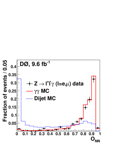
Figure 1 compares the NN output () distributions of photons and jets.
The shape of the distribution for photons is found to be in good agreement between
data and the MC simulation and is significantly different from the shape for misidentified
jets. The latter is validated using a sample enriched in jets misidentified as photons as
discussed in Sect. V.
Photon candidates are required to have a value larger than 0.1, which
is close to 100% efficient for photons while rejecting approximately 40% of the remaining misidentified jets.
Figure 1: Comparison of the normalized spectra for photons from DPP MC simulations and data events (points with statistical error bars), and
for misidentified jets from simulated dijet events.
The measured photon energies are calibrated using a two-step correction procedure.
In the first step, the energy response of the calorimeter to photons is calibrated using
electrons from boson decays. The resulting corrections are then applied to all
electromagnetic clusters. Since electrons and photons shower
differently, with electrons suffering from a larger energy loss in material
upstream of the calorimeter, the application of this first set of corrections results in an overestimate
of the photon energy which depends on .
In the second step, additional corrections are derived for photons reconstructed in
the central calorimeter using a detailed geant-based
simulation of the D0 detector response. These corrections are derived as a function
of photon transverse momentum () in seven intervals of : , ,
, , , , and , and
separately for photons with and without a matched CPS cluster.
The per-photon probability to have a matched CPS cluster is measured using photons radiated from charged
leptons in boson decays (, ) and is .
The finer binning at higher is motivated by the strong dependence of the
energy-loss corrections for electrons on .
The resulting corrections for photons with (without) a matched CPS cluster are
largest at low and range from about
in the interval, to about () in the interval.
IV.2 Primary vertex reconstruction
At the Tevatron the distribution of collision vertices has a Gaussian width of about 25 cm.
The proper reconstruction of the event kinematics, in particular and thus , requires the reconstruction and then correct selection of
the hard-scatter collision primary vertex (PV) among the various candidate
PVs originating from additional interactions.
The algorithm used for PV reconstruction is described
in detail elsewhere bidnim . In a first step, tracks with two or more associated SMT hits and
are clustered along the direction. This is followed by a Kalman Filter fit kalman to a common vertex
of the tracks in each of the different vertices. Events are required to have at least one reconstructed PV with
a coordinate () within 60 cm from the center of detector, a requirement that is efficient.
The selection of the hard-scatter PV from the list of PV candidates with cm
is based on an algorithm exploiting both the track multiplicity of
the different vertices and the transverse and longitudinal
energy distributions in the EM calorimeter and the CPS.
These energy distributions allow the estimation of the photon direction and thus
the coordinate of its production vertex along the beam direction.
When one or both photons reconstructed in the EM
calorimeter also deposit part of their energy in the
CPS, the algorithm chooses the PV whose is
closest to the extrapolation of the
photon trajectory determined from the calorimeter and
the CPS information pointing , provided the distance between
the coordinates of the vertex and of the photon
trajectory is smaller than 3 s.d.
The uncertainty on this distance is dominated by
the uncertainty on the extrapolation of the photon
direction, which ranges from cm for
photons with to cm for
photons with . Otherwise, the algorithm
chooses the PV with the largest
multiplicity of associated tracks.
This algorithm is optimized using data events,
where the correct hard-scatter PV associated with the
reconstructed tracks is treated as corresponding to a diphoton
event by ignoring the track information from the pair,
and added to the list of PV candidates to which the
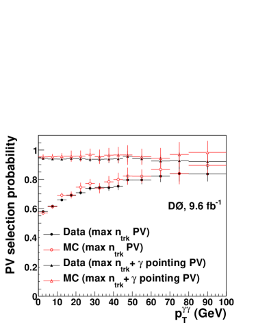
selection algorithm will be applied. The fraction of events for which
the selected PV agrees with the known hard-scatter PV is shown in Fig. 2
as a function of diphoton transverse momentum () for two different hard-scatter PV
selection algorithms. For an algorithm selecting the hard-scatter PV as the one with the highest track multiplicity,
the average selection probability is only
and shows a significant dependence on .
The improved algorithm used in this analysis, including also
photon pointing information, achieves an average selection probability
of , almost constant as a function of .
Figure 2: Probability to select the correct hard-scatter PV as a function of as measured
in events excluding the electron and positron tracks from consideration. The two
different algorithms discussed in the text are compared.
IV.3 Event selection
At least two photon candidates satisfying the requirements listed in Sect. IV.1 and having and are required.
If more than two photon candidates are identified, only the two photon candidates with highest are considered.
At least one of the photon candidates in each event is required to have a matched CPS cluster.
The photon kinematic variables are computed with respect to the vertex selected using the algorithm described in Sect. IV.2.
A requirement of is made to ensure a trigger efficiency close to 100%.
The acceptance of the kinematic requirements is , as estimated by applying the
and requirements to generated photons in a MC sample assuming .
At the same assumed , the overall event selection efficiency, taking into account acceptance and
reconstruction, identification and selection efficiencies, is , almost independent on the
signal production mechanism.
To improve the sensitivity to signal, events are categorized into two statistically independent samples with
different signal-to-background ratios. Events where both photon candidates satisfy (“photon-enriched” sample)
and events where at least one photon candidate satisfies (“jet-enriched” sample) are analyzed separately.
The corresponding sample compositions are discussed in Sect. V.
IV.4 Invariant mass reconstruction
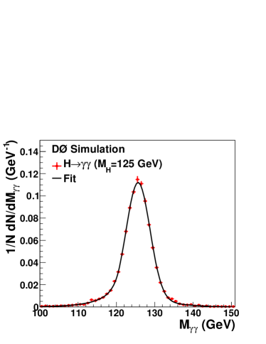
After the selection of the collision vertex and the photon energy scale corrections, the
distribution for a Higgs boson signal follows a Gaussian distribution peaking at the generated Higgs boson mass, with
small non-Gaussian tails. This distribution can be modeled by the sum of a Crystal Ball function CrystalBall ,
describing a narrow Gaussian core and a power-law tail toward lower masses, and a wider Gaussian distribution,
describing tails from misvertexing or imperfect photon energy scale corrections. Figure 3 shows such
a fit to the inclusive spectrum for signal MC with .
The resolution of the Gaussian core is found to be , and varies by when varying
by .
Figure 3: Distribution of the reconstructed diphoton invariant mass distribution corresponding to a Higgs boson signal with .
The line shows the result of a fit to the distribution using the functional form described in Sect. IV.4.
V Background modeling and sample composition
The normalization and shape of the background are estimated using
simulation. Electrons are misidentified as photons at a rate of about 2%
due to track reconstruction inefficiencies. Such tracking inefficiency is measured
in data using a “tag-and-probe” method, where events
are selected with one of the electrons (“tag”) passing all identification criteria,
including matching of the track to the calorimeter cluster, while only calorimeter requirements are applied to
the other electron (“probe”). The electron misidentification rate is computed
as the fraction of events where the probe electron satisfies the “track-match” veto requirement defined in Sect. IV.1.
The misidentification rate measured in data in this way is applied to the simulated sample.
The and yields are estimated using a data-driven method bkg-subtract (“matrix method”).
For selected events, the two photons are separated into two types: those with (well-identified photon, “p”) and those with (likely fake photon, “f”).
Events are then classified in four categories: (i) two type-p photons, (ii) the higher (leading) photon is type p and the lower (trailing) photon is type f,
(iii) the leading photon is type f and the trailing photon is type p, and (iv) two type-f photons.
The corresponding numbers of events, after subtracting the contribution,
are denoted as , , and .
The different efficiencies of the requirement for photons ()
and jets () are used to estimate the sample composition by solving a system of linear equations:
(1)
where () is the number of () events and ()
is the number of events with the leading (trailing) cluster as the photon.
The matrix is constructed with the efficiency terms
and , parameterized as a function of for each photon candidate as
determined from photon and jet MC samples, respectively. The and efficiencies averaged over are
and , respectively.
The efficiency is validated with a data sample of photons radiated from
charged leptons in boson decays (, ).
The efficiency is validated using two independent control data samples
enriched in jets misidentified as photons, either by inverting the photon isolation variable (), or
by requiring at least one track in a cone of around the photon diphoton-Xsection .
In the following, the sum of and contributions will be denoted as for simplicity.
The shapes of kinematic distributions for () background are obtained from
independent control samples by requiring one (two) photon candidate(s) to satisfy .
The requirement leads to a mis-modeling of the spectrum, due to
the dependence of . This is corrected by assigning a weight factor defined as /(1-)
for each of the photon candidates with .
As discussed in Sect. III, the kinematics of the DPP background are predicted using sherpa.
Since the estimated from solving Eq. 1 could
include a contribution from signal events, it is only used as a prior normalization for the DPP background
to compare between data and background prediction.
The normalization of the DPP background is ultimately determined from an unconstrained fit to
the final discriminants used for hypothesis testing in both the photon-enriched and jet-enriched samples.
For each of these samples, two distributions are considered: a multivariate discriminant (see Sect. VI) constructed to maximize
the separation between signal and background for events with falling in the interval (”search region”),
and the spectrum for events outside this interval (”sideband region”) that provide a high-statistics background-dominated
sample.
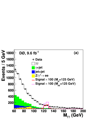
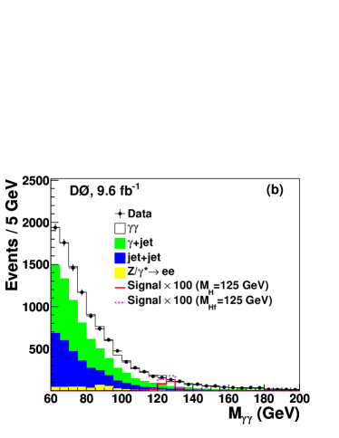
A comparison between data and the background prediction for the spectrum, separately in the
photon-enriched and the jet-enriched samples, is shown in Fig. 4.
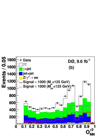
Figure 4: (color online). Distribution of in (a) the photon-enriched sample and (b) the jet-enriched sample.
The data (points with statistical error bars) are compared to the background prediction, broken down into its individual components.
The expected distributions for a SM Higgs boson and a fermiophobic Higgs boson with
are also shown scaled by a factor of 100.
Tables 1 and 2 summarize the number of data events,
expected backgrounds, and expected SM and fermiophobic Higgs boson signals, resulting from the fit for five hypothesized Higgs boson masses,
for the photon-enriched and jet-enriched samples, respectively.
For , the estimated background composition for the photon-enriched sample in the interval of [, ]
is about 80% (DPP), 14% (), 3% () and 3% ().
The corresponding composition for the jet-enriched sample is about 48% (DPP), 31% (), 18% () and 3% ().
(GeV)
105
115
125
135
145
(DPP)
2777 65
1928 44
1355 31
980 22
721 17
704 40
407 24
238 14
144 9
88 6
183 16
93 9
54 6
34 4
19 2
219 40
149 30
51 11
22 5
11 3
Total background
3883 61
2577 45
1698 30
1180 21
839 16
Data
3777
2475
1664
1147
813
signal
3.6 0.4
3.5 0.4
3.0 0.4
2.2 0.3
1.4 0.2
signal
49.8 1.1
14.0 0.3
4.8 0.1
1.9 0.1
0.79 0.03
Table 1: Signal, backgrounds and data yields for the photon-enriched sample within the mass window,
for to in intervals. The background
yields are from a fit to the data. The uncertainties include both statistical and systematic contributions added in quadrature and take into
account correlations among processes. The uncertainty on the total background is smaller than the sum in quadrature
of the uncertainties in the individual background sources due to the anti-correlation resulting from the fit.
(GeV)
105
115
125
135
145
(DPP)
1969 47
1406 33
1012 24
734 17
545 13
1852 100
1101 60
653 36
391 22
251 15
1188 94
647 54
365 31
219 19
135 12
227 39
152 28
61 11
30 7
20 5
Total background
5236 67
3307 45
2091 29
1374 21
951 17
Data
5287
3384
2156
1422
989
signal
2.7 0.3
2.6 0.3
2.2 0.3
1.7 0.2
1.1 0.1
signal
34.8 0.8
9.8 0.3
3.4 0.1
1.34 0.04
0.56 0.02
Table 2: Signal, backgrounds and data yields for the jet-enriched sample within the mass window,
for to in intervals. The background
yields are from a fit to the data. The uncertainties include both statistical and systematic contributions added in quadrature and take into
account correlations among processes. The uncertainty on the total background is smaller than the sum in quadrature
of the uncertainties in the individual background sources due to the anti-correlation resulting from the fit.
VI Signal-to-background discrimination
The diphoton mass is the most effective discriminating variable between the Higgs boson
signal and the background. However, further discrimination can be achieved
by exploiting additional kinematic variables as well as photon quality variables. A total
of ten well-modeled discriminating variables are considered in this search.
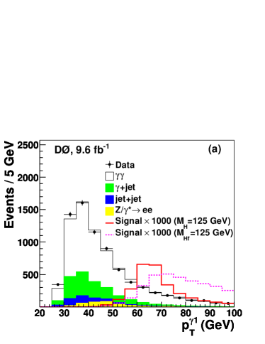
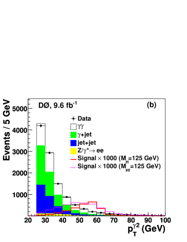
Two of these variables correspond to kinematic properties of the photons:
leading photon transverse momentum () and trailing photon transverse
momentum () which, as illustrated in Fig. 5, follow a
harder spectrum in signal than in background, as expected for the decay of a
heavy resonance.
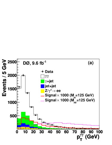
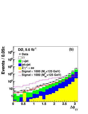
Three of the variables are related to the kinematics of the diphoton system:
, and azimuthal angle
separation between the photons (). The two latter variables give discrimination
due to the large of the Higgs boson in VH and VBF production. Therefore,
as illustrated in Fig. 6, and are particularly sensitive
variables in the search for a fermiophobic Higgs boson.
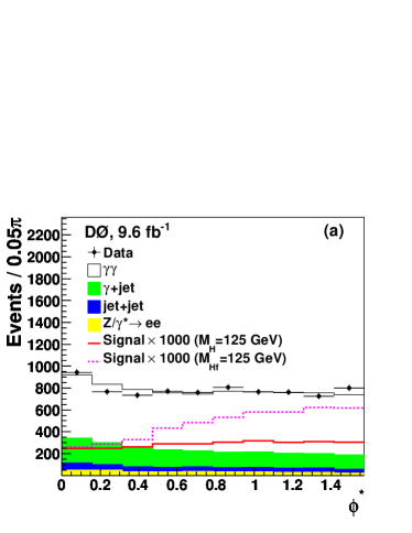
The scalar nature of the Higgs boson affects the angular distributions
of the photons in the diphoton rest frame. To minimize uncertainties from
the transverse momentum of the colliding partons, the Collins-Soper
frame collins-soper-frame is used. In this frame, the axis is defined
as the bisector of the proton beam momentum and the negative of the antiproton
beam momentum when they are boosted into the center-of-mass frame
of the diphoton pair. The variable is defined as the angle between the leading
photon momentum and the axis. The variable is defined as the angle
between the diphoton plane and the plane. Due to the restriction to photons with in
this analysis, the distribution has little discrimination between signal
and background, although it is considered in the search. In contrast, the angle
provides useful discrimination between signal and background, particularly
for a fermiophobic Higgs boson, as illustrated in Fig. 7(a).
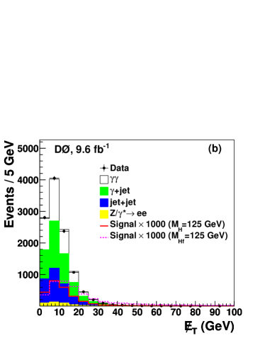
A significant fraction of and boson decays in VH production involves
neutrinos that result in large missing transverse energy () in the final state.
In contrast, the in background events is typically low, and mostly resulting
from jet energy mismeasurements. The distribution
in the jet-enriched sample is shown in Figure 7(b).
The is reconstructed as the negative of the vectorial sum of the
of calorimeter cells, and is corrected for the of identified muons
and the energy corrections to reconstructed jets in the calorimeter jets .
Figure 5: (color online). Distribution of (a) in the photon-enriched sample and (b) in the jet-enriched sample.
The data (points with statistical error bars) are compared to the background prediction, broken down into its individual components.
The expected distributions for a SM Higgs boson and a fermiophobic Higgs boson with
are also shown scaled by a factor of 1000.
These two BDT input variables are used in both the photon-enriched and jet-enriched samples, but are displayed here
for only one of the samples for illustrative purposes.
Figure 6: (color online). Distribution of (a) in the photon-enriched sample and (b) in the jet-enriched sample.
The data (points with statistical error bars) are compared to the background prediction, broken down into its individual components.
The expected distributions for a SM Higgs boson and a fermiophobic Higgs boson with
are also shown scaled by a factor of 1000.
These two BDT input variables are used in both the photon-enriched and jet-enriched samples, but are displayed here
for only one of the samples for illustrative purposes.
Figure 7: (color online). Distribution of (a) in the photon-enriched sample and (b) in the jet-enriched sample.
The data (points with statistical error bars) are compared to the background prediction, broken down into its individual components.
The expected distributions for a SM Higgs boson and a fermiophobic Higgs boson with
are also shown scaled by a factor of 1000.
These two BDT input variables are used in both the photon-enriched and jet-enriched samples, but are displayed here
for only one of the samples for illustrative purposes.
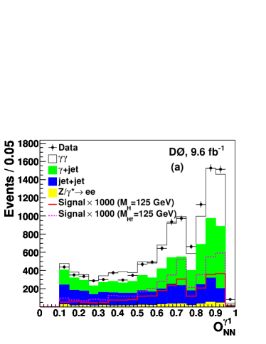
Figure 8: (color online). Distribution of (a) and (b) in the jet-enriched sample.
The data (points with statistical error bars) are compared to the background prediction, broken down into its individual components.
The expected distributions for a SM Higgs boson and a fermiophobic Higgs boson with
are also shown scaled by a factor of 1000.
These two BDT input variables are used as well in the photon-enriched sample, although their discrimination
power is limited given the requirement applied to both photons.
Finally, the distributions for the leading photon ()
and the trailing photon () show discrimination between
signal and the and backgrounds, in particular in the jet-enriched
sample, as illustrated in Fig. 8. The observed discrepancies between the
data and the total prediction in the shape of the distribution are partly covered by the
combination of statistical uncertainties on the templates and the systematic uncertainties,
and they have been checked to have a negligible impact on the final result.
To improve the sensitivity of the search, a boosted-decision-tree (BDT)
technique bdt is used to build a single discriminating variable combining the
information from the ten variables. A different BDT is trained, for each
hypothesis, for events selected in the search region, corresponding to
falling in the interval of .
The training is performed separately for the SM and the fermiophobic Higgs bosons
models, considering in each case the sum of all relevant signals against the
sum of all backgrounds. A separate BDT is trained in the photon-enriched and
jet-enriched samples, respectively. The resulting BDT output distributions assuming
a SM and a fermiophobic Higgs boson with are shown
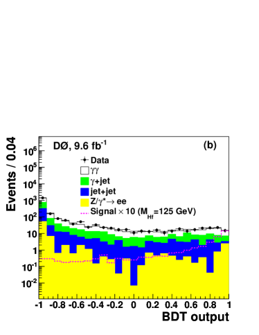
in Figs. 9 and 10, respectively. Prior to fitting the background
yields to the data, these distributions are well modeled by the simulation and no significant excess above
the background prediction is observed at high values of the BDT output.
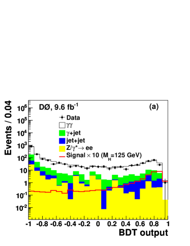
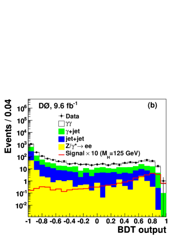
Figure 9: (color online). Distribution of the BDT output used in the SM Higgs boson search in (a) the photon-enriched sample and (b) the jet-enriched sample.
The data (points with statistical error bars) are compared to the background prediction, broken down into its individual components.
The expected distributions for a SM Higgs boson with are also shown
scaled by a factor of 10.
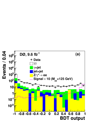
Figure 10: (color online). Distribution of BDT output used in the fermiophobic Higgs boson search in (a) the photon-enriched sample and (b) the jet-enriched sample.
The data (points with statistical error bars) are compared to the background prediction, broken down into its individual components.
The expected distributions for a fermiophobic Higgs boson with are also shown
scaled by a factor of 10.
VII Systematic uncertainties
Systematic uncertainties affecting the normalization and shape of the BDT output distributions
are estimated for both signal and backgrounds, taking into account correlations.
Experimental uncertainties affecting the normalization of the signal and the background
include the integrated luminosity (6.1%), tracking system live-time correction (2.0%), trigger efficiency (0.1%), PV reconstruction efficiency (0.2%),
and photon identification efficiency for signal (3.9%) or electron misidentification rate for (12.7%). The impact from PDF uncertainties
on the signal acceptance is 1.7%–2.2% depending on . Additional sources of uncertainty
affecting the normalization result from uncertainties on the theoretical cross section (including variations of the renormalization and factorization
scales signalscaleuncertainty and the PDFs pdfuncertainty ) for signal (GF (14.1%), VH (6.2%) and VBF (4.9%)) and (3.9%) production.
The normalization uncertainties affecting the and background predictions result from
propagating the uncertainties on (1.5%) and (10%)
in the estimation of their yields via Eq. 1. The uncertainties on the and yields
from varying are 6.9% and 5.3%, respectively. The corresponding uncertainties from varying
are 0.6% and 15.3%, respectively.
The remaining systematic uncertainties affect the shape of the BDT output distributions.
Such uncertainties include the photon energy scale (1%–5% for signal, 1%–4% for DPP background),
the modeling of DPP by sherpa (1%–10%), and the modeling
of the Higgs boson spectrum in GF production (1%–5%). The last two uncertainties
are obtained by doubling and halving the factorization and renormalization scales with respect to the
nominal choice. Uncertainties on the shape of the background are 5%–7% and are
estimated by comparing the BDT output distribution from the high-statistics samples obtained by inverting
the requirement to those predicted via the matrix method.
VIII Results
For each hypothesized value, the BDT output distributions discussed in Sect. VI for
the photon-enriched and jet-enriched samples are used to perform the statistical analysis to search
for a significant signal above the background prediction. As mentioned before, such discriminants
are defined only for events with falling in the interval.
The remainder of the spectrum (see Fig. 4) for both the photon-enriched and jet-enriched
samples, corresponding to the sideband regions, is also included in the statistical analysis as it
provides a significant constraint on the DPP normalization. Therefore, for each a total of four distributions are analyzed.
In the absence of a significant data excess above the background prediction, upper limits on the product of the
production cross section and branching fraction () are derived
as a function of , for both the SM and fermiophobic Higgs boson scenarios.
Limits are calculated at the 95% CL with the modified frequentist approach CLs-1 , which employs a log-likelihood ratio (LLR) as test-statistic,
, where () is a binned likelihood function (product
of Poisson probabilities) to observe the data under the signal-plus-background (background-only) hypothesis.
Pseudo-experiments are generated for both hypotheses, taking into account per-bin statistical fluctuations
of the total predictions according to Poisson statistics, as well as Gaussian fluctuations describing the effect of systematic uncertainties.
The individual likelihoods are maximized with respect to the DPP background normalization
as well as other nuisance parameters that parameterize the systematic uncertainties CLs-2 .
This global fit determines the normalization of the DPP background directly from data
and significantly reduces the impact of systematic uncertainties on the overall sensitivity.
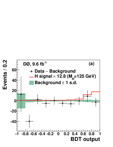
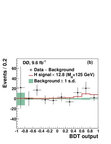
Examples of the post-fit BDT output distribution, after background subtraction, are shown in Fig. 11.
The fraction of pseudo-experiments for the signal-plus-background (background-only) hypothesis with LLR larger than a given
threshold defines (). This threshold is set to the observed (median) LLR for the observed (expected) limit.
Signal cross sections for which are deemed to be excluded at 95% CL.
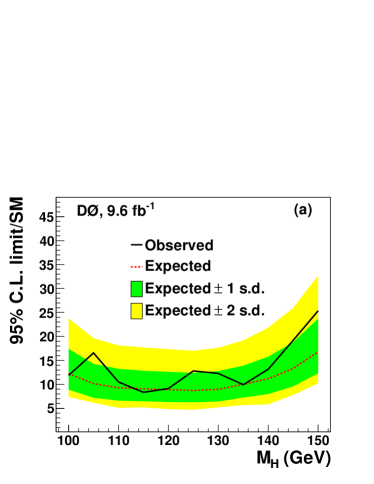
The resulting upper limits on relative to the SM prediction are shown
as a function of in Fig. 12(a), and are summarized in Table 3, representing the most constraining results
for a SM Higgs boson decaying into diphotons at the Tevatron.
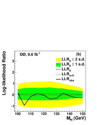
The corresponding LLR distribution is shown in Fig. 12(b). The observed local excesses of data are
under 2 s.d. and therefore are consistent with background fluctuations. At the best-fit
signal cross section is a factor of above the SM prediction. At the same mass, the value of is 0.72 while
the p-value for the background-only hypothesis is .
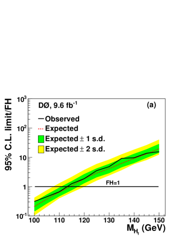
Upper limits on relative to the fermiophobic Higgs model prediction are shown
as a function of in Fig. 13(a), and are summarized in Table 4. This translates into the
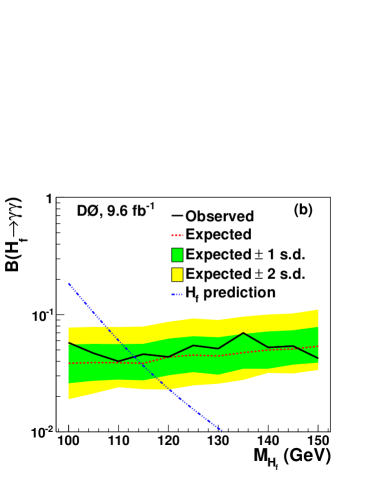
observed (expected) lower 95% CL of (114). After dividing by the theoretical cross section, upper limits on
are derived as a function of and presented in Fig. 13(b).
Figure 11: (color online).
Distribution of the BDT output for data (points with statistical error bars) after subtraction of the fitted background (under the background-only hypothesis) in (a) the photon-enriched sample and (b) the jet-enriched sample, for .
The expected SM Higgs signal is normalized to the observed limit on .
The bands represent the 1 s.d. uncertainties on the background prediction resulting from the fit.
Figure 12: (color online).
(a) Observed and expected 95% CL limits on the ratio of
to the SM prediction as a function of . The bands correspond to 1 and 2 s.d. around the median expected limit under the background-only hypothesis.
(b) Observed log-likelihood ratio (LLR) as a function of compared to the expected LLR under the background-only hypothesis (LLRb) and signal+background hypothesis (LLRs+b). The bands correspond to the 1 s.d. and 2 s.d. around the expected median LLRb.
Figure 13: (color online).
(a) Observed and expected 95% CL limits on the ratio of
to the fermiophobic Higgs model prediction as a function of .
The bands correspond to 1 and 2 s.d. around the median expected limit under the background-only hypothesis.
(b) Observed and expected 95% CL limits on as a function of .
The bands correspond to the 1 and 2 s.d. around the median expected limit under the background-only hypothesis.
Also shown is the prediction for a fermiophobic Higgs boson.
(GeV)
100
105
110
115
120
125
130
135
140
145
150
(fb)
Expected
46.1
37.2
32.8
30.3
27.7
24.6
22.0
20.7
18.7
17.2
15.9
Observed
44.7
60.6
37.1
27.9
28.4
36.1
30.1
20.5
22.0
24.8
24.0
/SM
Expected
12.2
10.2
9.3
9.1
8.9
8.7
9.0
10.0
11.2
13.3
16.8
Observed
11.9
16.6
10.5
8.3
9.1
12.8
12.3
9.9
13.2
19.2
25.4
Table 3: Expected and observed upper limits at 95% CL on the cross section times branching fraction for
() and on relative to the SM prediction for a SM Higgs
boson as a function of .
(GeV)
100
105
110
115
120
125
130
135
140
145
150
(fb)
Expected
20.9
18.3
15.9
13.7
13.6
12.4
10.8
10.2
9.5
8.6
8.1
Observed
31.3
22.0
16.3
16.4
13.7
15.0
12.5
15.0
10.0
9.1
6.4
Theoretical prediction
100.4
49.0
24.7
13.1
7.3
4.3
2.6
1.6
1.0
0.7
0.4
(%)
Expected
3.8
3.9
3.9
3.8
4.3
4.5
4.4
4.7
5.0
5.1
5.4
Observed
5.8
4.7
4.0
4.6
4.4
5.5
5.1
7.0
5.3
5.4
4.2
Theoretical prediction
18.5
10.4
6.0
3.7
2.3
1.6
1.1
0.8
0.5
0.4
0.3
Table 4: Expected and observed upper limits at 95% CL on the cross section times branching fraction for () and on for a fermiophobic Higgs boson as a function of . Also given are the theoretical predictions for
and as a function of .
IX Summary
A search for a Higgs boson decaying into a pair of photons has been presented using 9.6 fb-1 of collisions at
collected with the D0 detector at the Fermilab Tevatron Collider. The search employs multivariate
techniques to discriminate the signal from the non-resonant background, and is separately optimized
for a SM and a fermiophobic Higgs boson. No significant excess of data above the background prediction
is observed, and upper limits on the product of the cross section and branching fraction are derived at the 95% CL
as a function of . For a SM Higgs boson with , the observed (expected) upper limits
are a factor of 12.8 (8.7) above the SM prediction. The existence of a fermiophobic Higgs boson with mass in the 100–113
range is excluded at the 95% confidence level.
We thank the staffs at Fermilab and collaborating institutions,
and acknowledge support from the
DOE and NSF (USA);
CEA and CNRS/IN2P3 (France);
MON, NRC KI and RFBR (Russia);
CNPq, FAPERJ, FAPESP and FUNDUNESP (Brazil);
DAE and DST (India);
Colciencias (Colombia);
CONACyT (Mexico);
NRF (Korea);
FOM (The Netherlands);
STFC and the Royal Society (United Kingdom);
MSMT and GACR (Czech Republic);
BMBF and DFG (Germany);
SFI (Ireland);
The Swedish Research Council (Sweden);
and
CAS and CNSF (China).
References
(1)
S.L. Glashow, Nucl. Phys. 22, 579 (1961);
S. Weinberg, Phys. Rev. Lett. 19, 1264 (1967);
A. Salam, Proceedings of the 8th Nobel Symposium, ed. N. Svartholm, Almquist and Wiksel, Stockholm, 367 (1968).
(2)
F. Englert and R. Brout, Phys. Rev. Lett. 13, 321 (1964);
P.W. Higgs, Phys. Rev. Lett. 13, 508 (1964);
P.W. Higgs, Phys. Lett. 12, 132 (1964);
G. Guralnik, C. Hagen, and T. Kibble, Phys. Rev. Lett. 13, 585 (1964).
(4)
ALEPH, DELPHI, L3, and OPAL Collaborations, LEP Working Group for Higgs Boson Searches,
Phys. Lett. B 565, 61 (2003).
(5)
Tevatron New Physics and Higgs Working Group and CDF and D0 Collaborations, arXiv:1207.0449 [hep-ex].
(6)
T. Aaltonen et al. (CDF and D0 Collaborations), Phys. Rev. Lett. 109, 071804 (2012);
T. Aaltonen et al. (CDF Collaboration), Phys. Rev. Lett. 108, 151803 (2012);
V.M. Abazov et al. (D0 Collaboration), Phys. Rev. Lett. 108, 151804 (2012).
(7)
ATLAS Collaboration, Phys. Lett. B 716, 1 (2012).
(8)
CMS Collaboration, Phys. Lett. B 710, 26 (2012); Phys. Lett. B 716, 30 (2012).
(9)
S. Mrenna and J. Wells, Phys. Rev. D 63, 015006 (2000).
(10)
T. Plehn and M. Rauch, Europhys. Lett. 100, 11002 (2012).
(11)
A. Heister et al. (ALEPH Collaboration), Phys. Lett. B 544, 16 (2002);
P. Abreu et al. (DELPHI Collaboration), Eur. Phys. J. C 35, 313 (2004);
P. Achard et al. (L3 Collaboration), Phys. Lett. B 568, 191 (2003);
G. Abbiendi et al. (OPAL Collaboration), Phys. Lett. B 544, 44 (2002);
A. Rosca (LEP Collaborations), arXiv:hep-ex/0212038.
(12)
T. Aaltonen et al. (CDF Collaboration), Phys. Lett. B 717, 173 (2012).
(13)
V.M. Abazov et al. (D0 Collaboration), Phys. Rev. Lett. 107, 151801 (2011).
(14)
ATLAS Collaboration, Eur. Phys. J. C 72, 2157 (2012).
(15)
CMS Collaboration, J. High Energy Phys. 1209, 111 (2012).
(16)
V. M. Abazov et al., Nucl. Instrum. Methods Phys. Res. A 565, 463 (2006);
S. N. Ahmed et al., Nucl. Instrum. Methods Phys. Res. A 634, 8 (2011);
M. Abolins et al., Nucl. Instrum. Methods Phys. Res. A 584, 75 (2008);
R. Angstadt et al., Nucl. Instrum. Methods Phys. Res. A 622, 298 (2010).
(17)
Pseudorapidity is defined as , where is the polar angle
relative to the proton beam direction, and is the azimuthal angle in the plane transverse
to the proton beam direction.
(18)
T. Andeen et al., FERMILAB-TM-2365 (2007).
(19)
T. Sjöstrand et al., J. High Energy Phys. 05, 026 (2006).
Version 6.409 is used.
(20)
J. Pumplin et al., J. High Energy Phys. 07, 012 (2002);
D. Stump et al., J. High Energy Phys. 10, 046 (2003).
(21)
C. Anastasiou, R. Boughezal, and F. Petriello, J. High Energy Phys. 04, 003 (2009);
D. Florian and M. Grazzini, Phys. Lett. B 674, 291 (2009).
(22)
J. Baglio and A. Djouadi, J. High Energy Phys. 10, 064 (2010).
(23)
P. Bolzoni, F. Maltoni, S.O. Moch, and M. Zaro, Phys. Rev. Lett. 105, 011801 (2010).
(24)
A.D. Martin, W.J. Stirling, R.S. Thorne and G. Watt, Eur. Phys. J. C 63, 189 (2009).
(25)
A. Djouadi, J. Kalinowski, and M. Spira, Comput. Phys. Commun. 108, 56 (1998).
Version 3.70 is used.
(26)
G. Bozzi, S. Catani, D. de Florian, and M. Grazzini, Phys. Lett. B 564, 65 (2003);
Nucl. Phys. B737, 73 (2006).
(27)
T. Gleisberg et al., J. High Energy Phys. 02, 007 (2009).
Version 1.2.2 is used.
(28)
V.M. Abazov et al., (D0 Collaboration), arXiv:1301.4536 [hep-ex], submitted to Phys. Lett. B.
(29)
M.L. Mangano et al., J. High Energy Phys. 07, 001 (2003).
Version 2.11 is used.
(30)
V.M. Abazov et al., (D0 Collaboration), Phys. Rev. Lett. 100, 102002 (2008).
(31)
R. Hamberg, W.L. van Neerven and T. Matsuura, Nucl. Phys. B 359, 343 (1991) [Erratum-ibid. B 644, 403 (2002)].
(32)
R. Brun and F. Carminati, CERN Program Library Long Writeup W5013, 1993.
(33)
V.M. Abazov et al. (D0 Collaboration), Phys. Lett. B 659, 856 (2008).
(34)
V.M. Abazov et al. (D0 Collaboration), Phys. Rev. Lett. 102, 231801 (2009).
(35)
V.M. Abazov et al. (D0 Collaboration), Phys. Lett. B 653, 378 (2007).
(36)
V.M. Abazov et al. (D0 Collaboration), Nucl. Instrum. Methods Phys. Res. A 620, 490 (2010).
(40)
D. Acosta et al. (CDF Collaboration), Phys. Rev. Lett. 95, 022003 (2005).
(41)
V.M. Abazov et al., (D0 Collaboration), Phys. Lett. B 690, 108 (2010).
(42)
J.C. Collins and D.E. Soper, Phys. Rev. D 16, 2219 (1977).
(43)
G.C. Blazey et al., arXiv:hep-ex/0005012 (2000);
V.M. Abazov et al. (D0 Collaboration), Phys. Rev. D 85, 052006 (2012).
Calorimeter jets are reconstructed using the iterative midpoint cone
algorithm with radius in – space,
where is the rapidity.
(44)
A. Hoecker et al., arXiv:physics/0703039 [physics.data-an];
A. Hoecker et al., PoS (ACAT) 040 (2007).
(45)
I.W. Stewart and F.J. Tackmann, Phys. Rev. D 85, 034011 (2012).
(46)
S. Alekhin, S. Alioli, R.D. Ball et al., arXiv:1101.0536 [hep-ph];
M. Botje, J. Butterworth, A. Cooper-Sarkar et al., arXiv:1101.0538 [hep-ph].
(47)
T. Junk, Nucl. Instrum. Methods Phys. Res. A 434, 435 (1999); A. Read, J. Phys. G 28, 2693 (2002).