High-pressure, low-abundance water in bipolar outflows

Abstract

Context. Water is a potential tracer of outflow activity due to its heavy depletion in cold ambient gas and its copious production in shocks.

Aims. We present a survey of the water emission in a sample of more than 20 outflows from low mass young stellar objects with the goal of characterizing the physical and chemical conditions of the emitting gas.

Methods. We have used the HIFI and PACS instruments on board the Herschel Space Observatory to observe the two fundamental lines of ortho-water at 557 and 1670 GHz. These observations were part of the “Water In Star-forming regions with Herschel” (WISH) key program, and have been complemented with CO and H₂ data.

Results. The emission from water has a different spatial and velocity distribution from that of the $J$=1-0 and 2-1 transitions of CO. On the other hand, it has a similar spatial distribution to H₂, and its intensity follows the H₂ intensity derived from IRAC images. This suggests that water traces the outflow gas at hundreds of kelvins responsible for the H₂ emission, and not the component at tens of kelvins typical of low-$J$ CO emission. A warm origin of the water emission is confirmed by a remarkable correlation between the intensities of the 557 and 1670 GHz lines, which also indicates the emitting gas has a narrow range of excitations. A non-LTE radiative transfer analysis shows that while there is some ambiguity on the exact combination of density and temperature values, the gas thermal pressure $nT$ is constrained within less than a factor of 2. The typical $nT$ over the sample is $4\times 10^{9}$ cm^-3K, which represents an increase of $10^{4}$ with respect to the ambient value. The data also constrain within a factor of 2 the water column density, which varies over the sample from $2\times 10^{12}$ to $10^{14}$ cm^-2. When these values are combined with H₂ column densities, the typical water abundance is only $3\times 10^{-7}$, with an uncertainty of a factor of 3.

Conclusions. Our data challenge current C-shock models of water production due to a combination of wing-line profiles, high gas compressions, and low abundances.

1 Introduction

Bipolar outflows are ideal laboratories to study the physics and chemistry of interstellar medium shocks. They result from the interaction between a (still mysterious) supersonic wind launched by a protostar and the cold, extended gas cloud from which the protostar was born (Bachiller 1996; Arce et al. 2007). Their rich physical and chemical structure has attracted intense attention from both theorists and observers. Emission from H₂ vibration-rotation transitions, for example, reveals shock-heated gas at hundreds or few thousand kelvins (Gautier et al. 1976), while systematic abundance enhancements of species like SiO and CH₃OH evidences a rich chemistry driven by a combination of gas-phase reactions and dust shock disruption (van Dishoeck & Blake 1998). Both physical and chemical activity in outflows seem correlated with protostellar youth, likely due to the combined effect of outflow weakening with time and gradual clearing of the protostellar envelope (Bontemps et al. 1996; Tafalla & Bachiller 2011). As a result, the study of the physical and chemical activity of outflows is not only of interest for understanding ISM shocks, but constitutes a necessary step to elucidate the still-mysterious physics of star formation.

The H₂O molecule constitutes an exceptional tool for studying both the physics and chemistry of the shocked gas in outflows. H₂O has been found to be heavily depleted in the unperturbed gas of cold, star-forming regions (Bergin & Snell 2002; Caselli et al. 2012), and at the same time, is predicted to be copiously produced under the type of shock conditions expected in outflows (Draine et al. 1983; Kaufman & Neufeld 1996; Bergin et al. 1998; Flower & Pineau Des Forêts 2010). These extreme properties make H₂O a highly selective tracer of outflow activity, and indeed, H₂O maser emission has long been used as an outflow signpost, especially in high-mass star-forming regions (Genzel & Downes 1977). Unfortunately, maser emission, the only radiation from the H₂O main isotopologue observable from the ground, is a notoriously difficult tool for estimating emitting-gas parameters, since by its nature, it is highly biased to gas having specific, maser-producing physical conditions. To extract the full potential of H₂O as an outflow tracer, observations of its thermal emission are needed, and this requires the use of a space-based telescope.

The Infrared Space Observatory (ISO) provided the first systematic view of the thermal H₂O emission from outflows. The combined low angular and spectral resolution of the ISO data made it difficult to compare the observed H₂O emission with that of other tracers observable from the ground, like the low-$J$ transitions of CO. Still, these pioneer ISO observations revealed strong H₂O emission toward a number of young low-mass outflows from both the ground and excited energy levels, indicating that at least part of the H₂O emission originates in relatively warm gas (Liseau et al. 1996; Nisini et al. 1999; Giannini et al. 2001; Benedettini et al. 2002). Velocity-resolved H₂O observations were made possible first by the Submillimeter Wave Astronomy Satellite (SWAS) and later by Odin. These two satellites observed the fundamental line of ortho-H₂O at 557 GHz with velocity resolutions better than 1 km s^-1, revealing line profiles with high velocity wings of clear outflow origin (Franklin et al. 2008; Bjerkeli et al. 2009). However, neither SWAS nor Odin, with their several arcmin telescope beams, could resolve spatially the outflow emission, and these observations provided only a global view of the thermal emission from H₂O in outflows.

The Herschel Space Observatory (Pilbratt et al. 2010) has finally provided the combination of angular and spectral resolutions needed to study in detail the emission of H₂O in nearby outflows. Herschel instruments can observe a variety of ortho and para H₂O lines, opening up H₂O studies to the same multi-line type of analysis commonly used with other molecular tracers. To maximize this potential, the “Water In Star-forming regions with Herschel” (WISH) key program pooled more than 400 hr of telescope time with the goal of using H₂O and related molecules to study both the physical and chemical conditions of the gas in nearby star-forming regions (van Dishoeck et al. 2011). A specific subprogram of WISH is dedicated to study the H₂O emission from low-mass outflows, which are the ones most likely to show emission free from multiplicity and additional energetic phenomena. Due to the limited observing time available, the outflow subprogram was split into three parts with specific goals: (i) mapping three selected outflows to study the spatial distribution of H₂O, (ii) multi-transition observations toward two positions of each mapped outflow to constrain the H₂O excitation, and (iii) a survey of short integrations toward about 20 outflows to accumulate a statistically-significant sample of H₂O observations. Results from the mapping part of the program have been presented by Nisini et al. (2010a) for the L1157 outflow, Bjerkeli et al. (2012) for the VLA1623 outflow, and Nisini et al. (2013) for the L1448 outflow. Preliminary work on the multi-transition analysis has been presented by Vasta et al. (2012) for the L1157 outflow and Santangelo et al. (2012) for the L1448 outflow. In this paper, we report on the results of the statistical study of outflows. Additional results concerning outflow emission from different subprograms of WISH have been presented by Kristensen et al. (2011), Kristensen et al. (2012), and Herczeg et al. (2012) toward protostellar positions, and by Bjerkeli et al. (2011) toward the HH54 outflow region. Detailed observations of the L1157 outflow by the Chemical HErschel Surveys of Star forming regions (CHESS) program can be found in Lefloch et al. (2010), Codella et al. (2010), Benedettini et al. (2012), and Lefloch et al. (2012).

2 Observations

The survey presented here was designed as a first look at the H₂O emission from a large number of bipolar outflows using a moderate amount of telescope time (approximately 7 hours). This required a compromise between sample size, line selection, and sensitivity, and led to a strategy based on the observation of the two fundamental transitions of ortho-H₂O toward two positions in about 20 outflows, using a typical integration time of 300 seconds per transition.

2.1 Target selection

The survey target sample consists of 22 outflows, of which 17 are believed to be driven by class 0 sources, 3 are associated with class I sources, and 2 have driving sources of undetermined class (see Table 1 for central positions and Table 2 for the targeted outflow positions). Having a large fraction of class 0 sources was preferred because the outflows from these sources tend to be the most energetic and “chemically active” (Bontemps et al. 1996; Tafalla & Bachiller 2011), and were therefore expected to provide the highest rate of water detection. Intentionally, the list of exciting sources had a large overlap with the target list of the low-mass YSO subprogram of WISH, which studies the water emission from the envelopes of low-mass protostars (van Dishoeck et al. 2011; Kristensen et al. 2012). For most overlap sources, we selected one bright position in each outflow lobe generally well offset from the protostar, using as a guide published maps of emission from CO, SiO, or H₂. For sources with no overlap, we commonly chose the YSO as one of the survey targets, although the decision was made on a case-by-case basis taking into account the outflow geometry and our expectation for the brightest H₂O emission peak.

Given the diverse set of literature maps used to select the targets, our sample is not biased in a simple systematic way. It clearly represents a group of outflow positions likely to have strong H₂O emission, but our use of different tracers (CO, SiO, H₂) and literature maps of different quality and resolution made the sample significantly heterogeneous. As we will see below, the diverse nature of the sample became a significant advantage at the time of the analysis, because it increased the dynamic range of the observed intensities and probed (often inadvertently) a variety of emitting regions, and not just the brighter H₂O peaks.

After the survey was finished, we noticed that one target position had been erroneously associated with a bipolar outflow. This position corresponds to SERSMM4-B, and had been included in the sample because of the strong SiO and CH₃OH detections reported by Garay et al. (2002). Later CO(3–2) observations by Dionatos et al. (2010b), however, found no association of this position with the SERSMM4 outflow or with any other outflow from the Serpens cluster. To avoid contaminating our sample with a non-outflow position, the data from SERSMM4-B have been excluded from the analysis.

Table 1: Target outflows and central positions for offset calculation.⁽¹⁾

Source	$\alpha(J2000)$	$\delta(J2000)$	$V_{\mathrm{LSR}}$		$T_{\mathrm{bol}}^{(2)}$	Vel.
	$(\;^{h}\;{}^{m}\;{}^{s}\;)$	$(\;^{\circ}\;{}^{\prime}\;{}^{\prime\prime}\;)$	(km s-1)		(K)	Ref.
N1333I2	$03\;28\;55.6$	$+31\;14\;37$	7.	5	53	(3)
N1333I3	$03\;29\;03.8$	$+31\;16\;04$	7.	5	136	(3)
N1333I4A	$03\;29\;10.5$	$+31\;13\;31$	7.	2	34	(3)
HH211	$03\;43\;56.8$	$+32\;00\;50$	9.	1	30	(3)
IRAS04166	$04\;19\;42.6$	$+27\;13\;38$	6.	7	56	(4)
L1551	$04\;31\;34.1$	$+18\;08\;05$	6.	8	106	(3)
L1527	$04\;39\;53.9$	$+26\;03\;10$	5.	9	42	(3)
HH1-2	$05\;36\;22.8$	$-06\;46\;07$	9.	4	-	(5)
HH212	$05\;43\;51.4$	$-01\;02\;53$	1.	6	41	(6)
HH25MMS	$05\;46\;07.3$	$-00\;13\;30$	10.	3	47	(7)
HH111	$05\;51\;46.3$	$+02\;48\;30$	8.	7	69	(8)
HH46	$08\;25\;43.9$	$-51\;00\;36$	5.	3	112	(9)
BHR71	$12\;01\;36.3$	$-65\;08\;53$	-4.	5	48	(9)
HH54B	$12\;55\;50.3$	$-76\;56\;23$	2.	4	-	(10)
IRAS16293	$16\;32\;22.8$	$-24\;28\;36$	4.	0	45	(3)
L483	$18\;17\;29.9$	$-04\;39\;39$	5.	4	49	(3)
S68N	$18\;29\;48.0$	$+01\;16\;46$	8.	8	45	(3)
SERSMM1	$18\;29\;49.8$	$+01\;15\;21$	8.	5	39	(3)
SERSMM4	$18\;29\;56.6$	$+01\;13\;15$	8.	1	33	(3)
B335	$19\;37\;00.9$	$+07\;34\;10$	8.	3	42	(3)
N7129FIR2	$21\;43\;01.7$	$+66\;03\;24$	9.	5	52	(11)
CEPE	$23\;03\;13.1$	$+61\;42\;26$	-13.	0	56	(12)

• (1) All central positions as in van Dishoeck et al. (2011) except S68N, which has an offset of $9^{\prime\prime}$. See table 2 for the offsets of the observed positions; (2) Bolometric temperature as defined by Myers & Ladd (1993) and estimated using data from Spitzer telescope observations (Velusamy et al. 2007; Evans et al. 2009; Gutermuth et al. 2009; Rebull et al. 2010), AKARI (Ishihara et al. 2010; Yamamura et al. 2010), IRAS (Beichman et al. 1988; Hurt & Barsony 1996), and JCMT (Di Francesco et al. 2008); (3) Mardones et al. (1997); (4) Tafalla et al. (2004); (5) Marcaide et al. (1988); (6) Wiseman et al. (2001); (7) Choi et al. (1999); (8) Sepúlveda et al. (2011); (9) Bourke et al. (1995); (10) Bjerkeli et al. (2011); (11) Fuente et al. (2005); (12) Lefloch et al. (1996)

2.2 HIFI observations of H₂O(1₁₀–1₀₁)

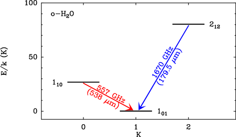
Figure 1: Lower part of the ortho-H₂O energy diagram illustrating the two transitions observed in the outflow survey. The colors of the arrows indicate the instruments used to observed the two transitions (red for HIFI and blue for PACS), and the energies of the levels are referred to the fundamental level of ortho-H₂O (instead of the frequently used para-H₂O).

We observed our target sources in H₂O(1₁₀–1₀₁) (rest frequency 556.9360020 GHz, Pickett et al. 1998, see Fig. 1) with HIFI (de Graauw et al. 2010) between April 2010 and April 2011. These observations, from now on referred to as the “557 GHz” observations, were done initially in position switching (PS) mode using a reference $10^{\prime}$ or more away from the source. Experience within the WISH project, however, showed that dual beam switching (DBS) with a $3^{\prime}$ chop produced flatter baselines than PS, and the observing mode was changed to DBS after the first set of data were obtained. In all observations, the local oscillator (LO) was tuned so that both H₂O(1₁₀–1₀₁) and NH₃($JK=10$–00) (rest frequency 572.4981599 GHz, Pickett et al. 1998) fell inside the bandpass. A few initial spectra had the NH₃ line (coming from the upper sideband) falling too close to the H₂O line (coming from the lower sideband), and the LO was re-tuned in the remaining observations to separate the lines and avoid possible overlaps.

During the observations, both the horizontal and vertical components of the polarization were detected, and the Wide Band Spectrometer (WBS) and High Resolution Spectrometer (HRS) were used to provide velocity resolutions of 0.6 and 0.13 km s^-1, respectively. The data were calibrated using the Standard Product Generation (SPG) pipeline in HIPE v6.1 (Ott 2010), and then converted to the GILDAS program CLASS for first order baseline subtraction, average of polarizations, and further processing. According to in-flight calibration measurements, the telescope beam size at 557 GHz was $39^{\prime\prime}$, and the beam efficiency was 0.76. (Roelfsema et al. 2012). All our intensities are expressed in $T_{\mathrm{mb}}$ units, with a nominal uncertainty estimated as $<15$%.

2.3 PACS observations of H₂O(2₁₂–1₀₁)

The observations of the H₂O(2₁₂–1₀₁) line (rest frequency 1669.9047750 GHz, Pickett et al. 1998, see Fig. 1) were carried out with the PACS instrument (Poglitsch et al. 2010) between October 2009 and September 2011 in line spectroscopy mode. This observing mode provided a $5\times 5$ array of velocity-unresolved spectra (FWHM $\approx 200$ km s^-1) covering a field of view of $47^{\prime\prime}\times 47^{\prime\prime}$. Each spectrum represents a sample on a $9\aas@@fstack{\prime\prime}4\times 9\aas@@fstack{\prime\prime}4$ pixel, which is slightly undersized compared to the $13^{\prime\prime}$ telescope beam at the operating frequency. The observations, from now on referred to as the “1670 GHz” observations, used the pointed chopping/nodding mode with a so-called large throw of $6^{\prime}$.

Depending on the date of the observation, the data were calibrated with HIPE versions 4, 5, or 6 using the standard reduction pipeline and a calibration scheme consistent among the HIPE versions. After that, the data were converted into CLASS format for first-order baseline subtraction and further analysis. To compare with the HIFI 557 GHz data, the PACS intensity scale of the 1670 GHz observations (Jy px^-1) was converted into an equivalent brightness temperature scale using the relation $T_{\mathrm{B}}(K)=5.6\>10^{-3}\;S_{\nu}$(Jy px^-1), which assumes square $9.4^{\prime\prime}$ pixels and an emitting region larger than the 13^′′ beam. A number of tests were carried out to ensure consistency between the calibration of PACS and HIFI data, including a comparison of intensities from objects observed in the 1670 GHz line with both instruments as part of different WISH subprograms. These and other tests carried out by the WISH team suggest that the uncertainty level of the PACS calibration is on the order of 20%.

2.4 Complementary IRAM 30m CO observations

Complementary observations of the Herschel targets were carried out with the IRAM 30m telescope between 2-4 May 2008. The observations consisted of CO(1–0) and CO(2–1) on-the-fly maps centered on the Herschel target position and covering a region $80^{\prime\prime}\times 80^{\prime\prime}$. Each mapping observation lasted about 15 minutes and was made in position-switching mode using the reference position initially chosen for the Herschel observations. Additional frequency switched spectra of most reference positions were taken to correct for possible contamination by residual emission. For each line, the two orthogonal polarizations were observed simultaneously and later averaged, and both the 1MHz filter bank and the VESPA autocorrelator were used as backends to provide velocity resolutions between 0.2 and 2.6 km s^-1. Data reduction was carried out with the CLASS software, and the intensity scale of the spectra was converted to $T_{\mathrm{mb}}$ using the facility-recommended efficiencies.

2.5 IRAC archival data

The IRAC instrument is a four-channel camera on the Spitzer Space Telescope that operates simultaneously at 3.6, 4.5, 5.8, and 8.0 $\mu$m with bandwidths between 0.8 and 3.0 $\mu$m (channels IRAC1 to IRAC4). It produces diffraction-limited images with a PSF between $1\aas@@fstack{\prime\prime}6$ and $1\aas@@fstack{\prime\prime}9$ depending on the wavelength (see Fazio et al. 2004 for a full description of the instrument). Over the years, IRAC has been used to observe most of our target objects as part of different projects, and all archival images are available at the Spitzer Heritage Archive (SHA). From this archive, we downloaded the Level 2 images of each target as reduced with the S18.18 pipeline, and we have used them to complement our H₂O analysis.

Being relatively broadband ($\sim 25$ %), the different IRAC channels are sensitive to both continuum and line emission. Of particular interest for our study are the lines from H₂, which include $v$ = 1-0 $O$(5)-$O$(7) and $v$ = 0-0 $S$(4)-$S$(13). In regions of shocked gas, these lines often dominate over the continuum contribution, making the IRAC images good tracers of the H₂ emission (Reach et al. 2006; Neufeld & Yuan 2008). As shown by Reach et al. (2006) and Neufeld & Yuan (2008), the $v$ = 1-0 lines lie inside the IRAC1 channel, and the $v$ = 0-0 lines are distributed over the four channels following a pattern of decreasing $S$ number with increasing wavelength. As a result of this order, the H₂ lines with lowest energy lie inside the IRAC4 passband, and this makes channel 4 of particular interest for our analysis. While this channel can suffer from potential contamination by PAH emission (Reach et al. 2006), the IRS spectra from Neufeld et al. (2009) show that even bright low-mass outflows like L1157, BHR71, or L1448 present negligible PAH features in the IRAC4 (6.5-9.5 $\mu$m) band. A comparison between IRAC1 and IRAC4 images for the objects of our sample shows no appreciable differences in the morphology of the emission, again suggesting that PAH contamination is negligible.

3 Overview of the survey results

Table 2: Survey positions and fit results.

		PACS(1)		HIFI(2)			PACS-HIFI(3)
Position	Offset(4)	$I$[1670 GHz]peak	Diam.	$I$[557 GHz]	$V_{\mathrm{LSR}}$	$\Delta V$	log[$N$(H2O)]	log($nT$)
	$(^{\prime\prime},\;^{\prime\prime})$	(K km s-1)	$(^{\prime\prime})$	(K km s-1)	(km s-1)	(km s-1)	(cm-2)	(cm-3 K)
N1333I2-B	$(-103,+23)$	3.5 (0.6)	30 (4.8)	6.34 (0.04)	-0.14 (0.04)	11.3 (0.08)	13.4 (0.2)	9.2 (0.1)
N1333I2-R	$(+67,-17)$	5.5 (0.8)	22 (2.3)	7.15 (0.06)	14.0 (0.07)	14.2 (0.1)	13.3 (0.2)	9.4 (0.1)
N1333I3-B2	$(+20,-50)$	1.7 (0.2)	27 (3.1)	2.65 (0.07)	2.0 (0.3)	20.5 (0.6)	12.8 (0.2)	9.4 (0.1)
N1333I3-B1	$(+20,-20)$	5.9 (1.4)	18 (2.9)	5.35 (0.08)	-4.6 (0.2)	25.4 (0.4)	13.1 (0.1)	9.7 (0.1)
N1333I4A-B	$(-6,-19)$	14.0 (2.9)	34 (6.8)	15.0 (0.1)	1.3 (0.06)	17.4 (0.1)	13.5 (0.1)	9.1 (0.1)
N1333I4A-R	$(+13,+25)$	9.3 (1.2)	28 (3.5)	7.76 (0.07)	13.3 (0.09)	19.3 (0.2)	13.4 (0.1)	9.7 (0.1)
HH211-R	$(-37,+15)$	2.8 (0.6)	28 (5.8)	-	No data	-	-	-
HH211-C	$(0,0)$	11.7 (1.6)	17 (1.7)	6.53 (0.02)	11.5 (0.07)	41.4 (0.1)	13.2 (0.1)	9.8 (0.1)
HH211-B	$(+37,-15)$	7.7 (1.0)	14 (1.3)	2.33 (0.06)	6.2 (0.3)	20.0 (0.7)	12.8 (0.1)	10.1 (0.1)
IRAS04166-R	$(-20,-35)$	No data	No data	0.27 (0.05)	13.0 (0.7)	9.1 (2.4)	-	-
IRAS04166-B	$(+20,+35)$	Bad fit	Bad fit	0.53 (0.04)	0.0 (0.4)	10.0 (1.1)	12.4 (0.3)	9.2 (0.1)
L1551-B	$(-255,-255)$	Bad fit	Bad fit	0.36 (0.03)	-3.2 (0.2)	5.9 (0.5)	12.3 (0.2)	9.2 (0.1)
L1551-R	$(+150,+20)$	1.3 (0.2)	13 (1.4)	0.58 (0.04)	7.8 (0.3)	5.7 (0.6)	12.4 (0.1)	9.7 (0.1)
L1527-B	$(+40,+10)$	No data	No data	0.93 (0.07)	9.3 (0.8)	20.3 (2.1)	-	-
HH1	$(-30,+55)$	2.9 (0.3)	13 (1.0)	-	No data	-	-	-
HH2	$(+60,-80)$	3.5 (0.5)	30 (4.4)	2.4 (0.05)	9.8 (0.2)	17.7 (0.4)	12.9 (0.1)	9.7 (0.1)
HH212-B	$(-15,-35)$	0.4 (0.1)	37 (13)	0.76 (0.04)	1.1 (0.2)	8.4 (0.5)	12.3 (0.1)	9.5 (0.1)
HH212-C	$(0,0)$	2.5 (0.4)	18 (1.9)	2.3 (0.07)	2.6 (0.4)	23.2 (0.8)	12.6 (0.1)	9.8 (0.1)
HH25-C	$(0,0)$	12.5 (0.9)	14 (0.7)	5.2 (0.06)	12.4 (0.09)	16.6 (0.3)	13.1 (0.1)	9.9 (0.1)
HH25-R	$(+36,-57)$	3.2 (0.4)	36 (4.4)	4.9 (0.07)	11.2 (0.04)	6.9 (0.09)	13.1 (0.2)	9.5 (0.1)
HH111-B	$(-170,+21)$	0.3 (0.1)	34 (11)	-	Bad fit	-	-	-
HH111-C	$(0,0)$	2.0 (0.3)	12 (1.3)	0.54 (0.05)	9.3 (0.6)	14.6 (1.6)	12.4 (0.1)	9.9 (0.1)
HH46-R	$(-40,-20)$	0.8 (0.2)	35 (7.3)	-	No data	-	-	-
HH46-B	$(-10,0)$	No data	No data	1.54 (0.06)	10.8 (0.4)	20.0 (1.0)	-	-
BHR71-R	$(-39,+140)$	1.9 (0.2)	46 (5.5)	7.0 (0.08)	3.0 (0.1)	16.1 (0.2)	13.4 (0.5)	8.8 (0.4)
BHR71-B	$(+42,-100)$	2.7 (0.3)	32 (3.4)	3.4 (0.06)	-6.4 (0.07)	7.5 (0.2)	13.6 (0.7)	8.9 (0.6)
HH54B(5)	$(2,4)$	8.8 (0.4)	22 (0.8)	10.6 (0.07)	-6.6 (0.05)	14.5 (0.1)	13.3 (0.1)	9.6 (0.1)
IRAS16293-B	$(+72,-56)$	0.1 (0.2)	13 (16)	1.6 (0.05)	1.7 (0.06)	3.6 (0.1)	-	-
IRAS16293-R	$(+72,+49)$	0.8 (0.1)	38 (6.2)	6.2 (0.04)	8.2 (0.03)	9.7 (0.07)	14.1 (0.2)	7.8 (0.2)
L483-B	$(-60,+30)$	0.4 (0.2)	21 (6.3)	0.70 (0.05)	1.4 (0.5)	12.7 (1.0)	13.6 (0.6)	8.0 (0.5)
S68N-B	$(-12,+24)$	6.9 (0.5)	23 (1.6)	4.5 (0.07)	6.1 (0.1)	15.5 (0.4)	13.2 (0.1)	9.6 (0.1)
S68N-C	$(0,0)$	8.9 (1.2)	31 (3.6)	10.9 (0.07)	9.1 (0.05)	17.6 (0.2)	13.2 (0.1)	9.8 (0.1)
SERSMM1-B	$(-18,+30)$	8.8 (0.8)	21 (1.9)	4.5 (0.09)	10.0 (0.2)	22.6 (0.9)	13.2 (0.1)	9.7 (0.1)
SERSMM4-B	$(-60,+30)$	0.4 (0.2)	18 (10)	1.9 (0.03)	5.0 (0.04)	5.7 (0.1)	13.9 (0.2)	7.6 (0.4)
SERSMM4-R(6)	$(+30,-60)$	0.4 (0.1)	44 (21)	1.9 (0.05)	11.6 (0.2)	13.2 (0.6)	13.1 (0.6)	8.6 (0.5)
B335-B	$(+30,0)$	No data	No data	-	Bad fit	-	-	-
N7129FIR2-R	$(+50,-50)$	0.3 (0.2)	19 (7.1)	-	Bad fit	-	-	-
CEPE-B	$(-12,-20)$	71.2 (7.7)	15 (1.1)	26.2 (0.2)	-27.4 (0.2)	44.6 (0.4)	13.9 (0.1)	10.0 (0.1)
CEPE-R	$(+8,+20)$	27.7 (3.4)	22 (2.1)	-	No data	-	-	-

• (1) PACS results from gaussian fits to the radial profiles of integrated intensity with rms uncertainty values in parenthesis. The origin of the profile is the emission centroid and the diameter is the FWHM of the fitted gaussian (without correction for the $13^{\prime\prime}$ telescope beam); (2) HIFI results from gaussian fits to the spectra with rms uncertainty values in parenthesis. $\Delta V$ represents the FWHM of the emission; (3) Results from the analysis of the combined PACS and HIFI data toward the emission peak and with a resolution of $13^{\prime\prime}$, see Sect. 7.2; (4) Offsets are with respect to the central position in Table 1; (5) Data previously published by Bjerkeli et al. (2011); (6) Position excluded from sample analysis due to dubious outflow origin.

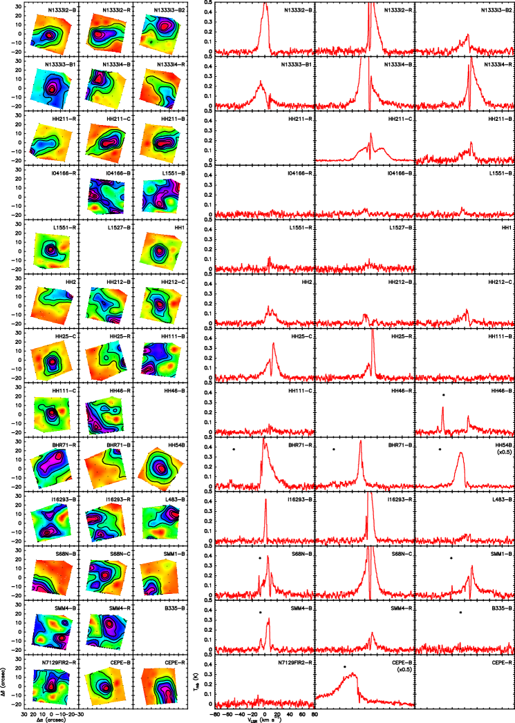
Figure 2: Summary view of all the outflow survey data ordered by increasing right ascension, as in Table 2. Left panels: PACS maps of H₂O(2₁₂–1₀₁) integrated intensity showing contours at 20, 40, 60, 80, and 90% of the peak value (see Table 2 for absolute intensities). The points indicate the location of the individual PACS spaxels. Right panels: HIFI spectra of H₂O(1₁₀–1₀₁) with fixed intensity and velocity scales for easier inter-comparison (some bright spectra have been scaled down to fit the box). Asterisk signs in some spectra indicate the position of the NH₃($JK$=10–00) line coming from the upper sideband of the receiver. Empty boxes correspond to positions observed with one instrument but not with the other.

Fig. 2 presents a summary view of all the data from the outflow survey. The left block of panels shows the PACS results in the form of $5\times 5$ integrated-intensity maps using contours proportional to the map peak intensity. The right block of panels presents the HIFI spectra with fixed scale in both velocity and intensity. In total, 39 different positions were observed in at least one of the two H₂O lines, and 32 positions were observed with both PACS and HIFI (some positions were dropped during the survey due to weak emission and time limitations).

As the figure illustrates, the objects in the sample present a diversity of spatial distributions and intensities. The PACS maps show that the 1670 GHz emission tends to be spatially concentrated, but that it usually extends over scales larger than the $13^{\prime\prime}$ PACS beam. The emission peaks do not always coincide with the central position of the map, which corresponds to our expected location for the H₂O maximum. An object-by-object inspection shows that this mismatch arises from a combination of errors in the literature maps used to prepare the observations and true offsets between the peaks of the H₂O emission and the peaks of the molecular emission used to choose the PACS map center (usually CO). The origin of these offsets will be further explored below.

Less clear from the PACS maps due to the use of relative contours is the large range of intensities covered by the sample. This is better appreciated from the HIFI spectra, which cover almost two orders of magnitude in integrated intensity between the brightest (CEPE-B) and weakest (L1551-B) 557 GHz lines. A large intensity range must be intrinsic to the sample, and cannot arise solely from errors in predicting the peak position, or from beam dilution effects, since sources like L1551-R or HH111-C present very weak HIFI spectra despite their emission being well centered on the PACS maps. As we will see below, the large range in integrated intensities seems to arise from an equivalent large range of H₂O column densities in the sample. This means that although the target selection was biased toward bright H₂O candidates, the sample has still almost two orders of magnitude of dynamic range, which gives a convenient margin to explore different emission conditions and optical depth effects in the targets.

Also noticeable in the HIFI data are the diversity of linewidths and spectral shapes. As previously noticed by Kristensen et al. (2012) in their observations toward the low-mass YSO themselves, most 557 GHz lines present a narrow dip at ambient velocities that likely arises from self-absorption by low-excitation H₂O along the line of sight (see Caselli et al. 2012 for a study of ambient H₂O emission and absorption in dense cores). An additional narrow feature appears at shifted velocities toward a number of spectra taken in the first batch of observations, like HH46-B. It results from the superposition of NH₃(10–00) emission, coming from the upper sideband of the receiver, and its position has been indicated by an asterisk in those spectra where it appears. Apart from these two narrow features, the HIFI spectra are dominated by broad wings typical of outflow emission.

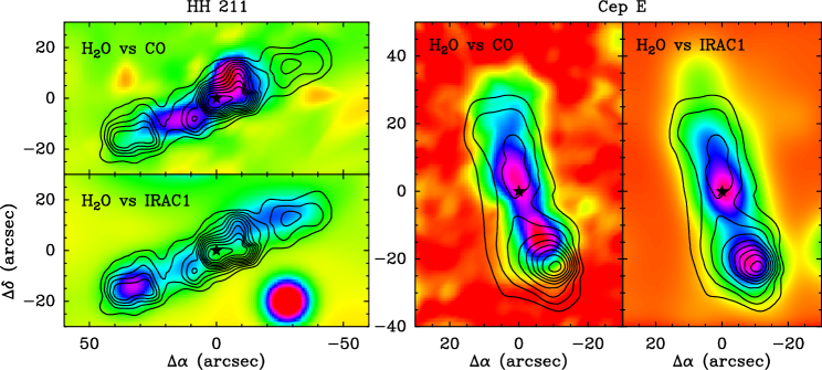
Figure 3: Comparison between H₂O(1670 GHz) integrated intensity (contours) and either CO(2–1) or H₂-dominated IRAC1 images (color-coded background) for the HH 211 and Cepheus E outflows. The IRAC1 image has been convolved to a resolution of $13^{\prime\prime}$ to match the resolution of the H₂O(1670 GHz) and CO(2–1) data. For H₂O(1670 GHz), first contour and contour interval are 1 K km s^-1 for HH211 and 8 K km s^-1 for Cep E. The CO map of HH211 uses data presented in Tafalla et al. (2006), and represents CO(2–1) intensities integrated in the velocity range $|V-V_{0}|\leq 5-20$ km s^-1 (ambient cloud velocity $V_{0}=8.6$ km s^-1). The CO map of Cep E represents CO(2–1) intensities integrated in the range $|V-V_{0}|\leq 10-50$ km s^-1 (ambient cloud velocity $V_{0}=-13$ km s^-1), and has been shifted by $5^{\prime\prime}$ to the west to correct for a possible pointing problem suggested by an overlap with the better-registered interferometer map of Moro-Martín et al. (2001). Note the better agreement of the H₂O with the H₂-dominated IRAC1 emission than with the CO(2–1) emission. In all plots, the star symbol indicates the position of the YSO, which is the origin of the offset values and whose absolute coordinates are given in Table 1. The bright circular feature near ($-30^{\prime\prime}$, $-20^{\prime\prime}$) in the HH 211 IRAC1 image corresponds to an unrelated star.

The maps and spectra in Fig. 2 also illustrate the complementarity of the PACS and HIFI observations. The PACS data lack velocity resolution, but provide information about the spatial distribution of the H₂O emission. They do this with a relatively high angular resolution of $13^{\prime\prime}$ over a region of $47^{\prime\prime}\times 47^{\prime\prime}$. The single-pixel HIFI data, on the other hand, do not provide spatial information, but have a velocity resolution of 0.6 km s^-1. The beam size of the HIFI data ($39^{\prime\prime}$) is similar to the field of view of the PACS observations, so the HIFI velocity-resolved spectra correspond to an emitting region approximately the size of the PACS maps. The goal of the analysis presented here is to combine the spatial and velocity information provided by PACS and HIFI into a self-consistent picture of the H₂O emission from outflow gas. As we will see in Sect. 6.1, this approach is justified by the tight correlation between the intensities of the 557 and 1670 GHz lines, which argues strongly for the two transitions arising from the same volume of gas. Before combining the PACS and HIFI observations, however, we study the two sets of observations separately and characterize the spatial and velocity properties of the H₂O emission.

4 PACS data: spatial information

4.1 Two illustrative outflows: HH 211 and Cepheus E

Our survey observations were not designed to map the full H₂O emission from outflows, which is often extended and requires dedicated on-the-fly observations. A separate effort inside the WISH project was dedicated to map a selected number of outflows, and initial results have already been presented (Nisini et al. 2010a; Bjerkeli et al. 2012; Nisini et al. 2013). The outflows from the targets HH 211 and Cepheus E, however, are compact enough to be covered with two or three PACS fields of view, so our observations provide full maps of the 1670 GHz H₂O emission in these systems. Although not as finely sampled as the dedicated on-the-fly maps, these small PACS maps can be used to study the relation between the H₂O emission and the emission from other outflow tracers, in particular CO and H₂.

Previous observations of HH 211 and Cepheus E have shown that the two outflows share a common feature. Their emission in low-$J$ CO transitions peaks significantly closer to the protostar than their H₂ emission, which is brighter toward the end of the outflow lobes. This offset between the H₂ and low-$J$ CO emitting regions is specially noticeable in the maps of HH 211 by McCaughrean et al. (1994) (their Fig. 6) and Cepheus E by Moro-Martín et al. (2001) (their Fig. 9). It most likely results from the outflows having at least two spatially-separated components of different temperature, with the H₂-emitting gas being significantly hotter than the low-$J$ CO-emitting gas (Moro-Martín et al. 2001). This stratification of the outflow emission makes HH 211 and Cepheus E ideal targets to probe the gas conditions traced by the H₂O emitting gas, and in particular, to distinguish between an origin in gas with low excitation (CO-like) and high excitation (H₂-like).

Fig. 3 presents a comparison between the emission from H₂O and that of CO and the H₂-dominated IRAC1 band toward HH 211 and Cepheus E. In all panels, the contours represent the integrated intensity of the PACS-observed H₂O(1670 GHz) line, while the color backgrounds are the CO(2–1) IRAM 30m emission in the “H₂O vs CO” panels and the Spitzer/IRAC1 emission in the “H₂O vs IRAC1” panels. All the data have similar angular resolution, since the IRAC1 image has been convolved with a $12^{\prime\prime}$ gaussian, and both the H₂O and CO data have intrinsic resolutions of $12-13^{\prime\prime}$.

As can be seen, the H₂O emission from HH 211 presents three separate peaks, one toward the YSO and one toward the end of each outflow lobe. The CO emission, on the other hand, has a bipolar distribution that consists of two peaks approximately located half way between the central source and the outer H₂O peaks. While not completely anti-correlated, the H₂O and CO emissions clearly do not match and their peaks seem to avoid each other. In contrast with CO (and in agreement with NIR H₂ images), the H₂-dominated IRAC1 emission peaks further from the YSO and matches better the H₂O emission at the end of the two lobes, especially toward the brightest south-east end of the outflow. No IRAC emission is seen toward the central H₂O peak, but this may result from strong extinction, since even the protostellar continuum is invisible in the IRAC bands.

The better match between the H₂O and IRAC1 emissions is also noticeable in Cepheus E (Fig. 3 right panels). As in HH 211, the CO emission from the southern outflow lobe lies closer to the YSO than the H₂O emission, while the IRAC1 emission matches well the bright southern H₂O peak. Less clear is the comparison toward the northern lobe, since all emissions drop gradually away from the YSO (the IRAC emission toward the YSO is likely contaminated by protostellar continuum, see Noriega-Crespo et al. 2004). In any case, the maps in Fig. 3 show that the H₂O emission from Cepheus E is, like in HH 211, more H₂-like than CO-like.

A more quantitative comparison between the H₂O, CO, and H₂ emissions is presented in Fig. 4 using intensity cuts along the outflow axes for both the eastern lobe of HH 211 and the southern lobe of Cepheus E. These two lobes present the brightest H₂O and H₂ intensities (McCaughrean et al. 1994; Moro-Martín et al. 2001), and are therefore the best regions for a comparison between the different outflow tracers. As can be seen, the H₂O and H₂ emissions (blue and green lines) peak approximately at the same distance from the YSO and have similar widths, while the CO emission (red line) peaks closer to the YSO by $15^{\prime\prime}$ in HH 211 and $10^{\prime\prime}$ in Cepheus E. The close match between the H₂O and H₂ spatial profiles indicates that the gas conditions responsible for the two emissions must be rather similar, while they must differ significantly from the conditions of the gas responsible for the CO(2–1) emission. This is a first indication that the H₂O-emitting gas in the outflow lobes has a higher excitation than the low-$J$ CO-emitting gas commonly associated with outflow material.

4.2 A general correlation between the H₂O and H₂ emissions

The spatial correlation between the H₂O and H₂ emissions is not limited to the HH211 and Cep E outflows just studied, but seems to extend to the whole sample. A one-by-one comparison between the PACS maps of Fig. 2 and equivalent IRAC images from the Spitzer archive shows that in most cases the H₂O emission matches spatially that of H₂, even when the H₂ and the low-$J$ CO emissions differ in their distribution (like seen in HH 211 and Cep E). The PACS H₂O maps are therefore systematically “H₂-like” both in peak location and spatial extent, and this suggests that the conditions of the gas responsible for the H₂O emission are similar to those of the H₂-emitting gas.

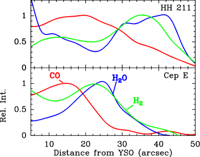
Figure 4: Spatial profiles of the emission from Fig. 3 along the eastern lobe of HH 211 (top) and southern lobe of Cepheus E (bottom). The blue lines represent the 1670 GHz H₂O emission, the green lines represent H₂-dominated IRAC1 emission, and the red lines correspond to CO(2–1). All data have a similar resolution of approximately $13^{\prime\prime}$.

The similar spatial distribution of the H₂O and H₂ emissions was not recognized at the time of target selection (circa 2007), and this explains why a number of PACS maps in Fig. 2 appear offset or even miss the H₂O peak. Target selection in our survey was mainly guided by low-$J$ CO maps, so most PACS centers were chosen to coincide with the peak of this relatively low excitation emission. L483 provides a good illustration of this issue, since in this outflow the H₂ peak is known to lie more than $20^{\prime\prime}$ to the west of the CO peak (Fuller et al. 1995; Tafalla et al. 2000). As Fig. 2 shows, our CO-centered PACS map misses a significant part of the H₂O emission, which extends to the west of our chosen field of view. Although unfortunate, the sometimes dramatic effect of our shifted target selection has helped to highlight the H₂-like nature of the H₂O emission. It also has made our H₂O survey cover not only the bright emission peaks but the more extended component.

A notable exception to the good match between PACS and IRAC images is the NGC 1333-I2 outflow. The PACS maps of this source present two bright H₂O peaks that coincide with the CO/CH₃OH/SiO outflow maxima east and west of the YSO (Sandell et al. 1994; Bachiller et al. 1998; van Dishoeck & Blake 1998; Jørgensen et al. 2004), while no H₂ emission from either H₂O peak can be discerned in the IRAC images. Although this may indicate an anomalous behavior of the NGC 1333-I2 outflow, it more likely results from high extinction inside the NGC 1333 star-forming dense core. This interpretation is supported by the scarcity of background stars seen by IRAC and by the recent observations at longer wavelengths by Maret et al. (2009). These authors found a bright H₂ $S(1)$ 17$\mu$m emission peak toward the eastern lobe of NGC 1333-I2 with similar shape and size to the H₂O peak seen in the PACS map. Such detection of $S(1)$ emission indicates that at least the eastern lobe of the NGC 1333-I2 outflow is associated with a significant amount of excited H₂, and that if this emission is not seen in the IRAC images, it is likely due to an extreme case of extinction similar to that occurring at center of the HH211 outflow. Unfortunately, Maret et al. (2009) did not cover the western lobe of the outflow in their map, so the status of this position remains uncertain.

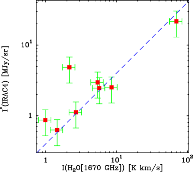
Figure 5: Comparison between extinction-corrected IRAC4 intensities and H₂O(1670 GHz) integrated intensities for the sources of Table 3. The formal error bars assume a 40% uncertainty in the IRAC4 intensities (due to the accumulated uncertainty of background subtraction and extinction correction) and a 20% uncertainty in the PACS intensities. The dashed line is a linear correlation that, according to the analysis of section 8.1, corresponds to a constant H₂O abundance value of $3\times 10^{-7}$.

The correlation between the H₂ and H₂O emissions is not limited to morphology, but involves line intensities. Comparing the intensities in the PACS and IRAC images, however, is not a straightforward operation, since the IRAC intensities represent more than just H₂ emission. They contain possible contributions from continuum emission from YSOs and unrelated objects together with diffuse background radiation from the cloud (plus the already mentioned non-negligible dust extinction in dense regions). To minimize these effects, we limit our PACS-IRAC comparison to the peak values of positions where the IRAC emission can be reasonably expected to have uncontaminated H₂ origin and to be associated with the H₂O emission seen with PACS. We have done this by selecting the sources whose well-defined PACS maximum is offset more than $10^{\prime\prime}$ from the YSO position (to avoid protostellar continuum contribution in the IRAC images). For these sources, we have convolved the IRAC images with a gaussian to simulate the $13^{\prime\prime}$ resolution of the PACS observation, and used this convolved image together with the PACS map to estimate the H₂ and H₂O intensities at the peak. In order to subtract the extended emission contribution (important in the IRAC images) we have measured in each image the intensities at three different positions: the H₂O(1670 GHz) peak and two off-peak positions that seem unaffected by protostellar or background contamination. The average intensity of these off-center positions is used to estimate a background contribution, which is then subtracted from the peak intensity. A further correction of the IRAC intensity for dust extinction is made using literature values of A_V extrapolated to the IRAC wavelengths, assuming A_K/A_V = 0.112 (Rieke & Lebofsky 1985) and the A_λ/A_K ratios recommended by Indebetouw et al. (2005).

Table 3: H₂O(1670 GHz)-IRAC4 correlation

Source	$I$[H2O(1670 GHz)]	$I$[IRAC4]	AV	AV Ref.
	(K km s-1)	(MJy sr-1)	(mag)
N1333I3-B2	2.2	3.4	9	(1)
N1333I3-B1	5.4	2.1	9	(1)
HH211-B	5.7	1.7	8	(2)
HH1	2.7	1.1	1.5	(1)
HH46-R	1.0	0.6	8	(3)
BHR71-R	1.5	0.6	1	(4)
CEPE-B	70.3	12.5	12.5	(5)
HH54	8.5	2.3	2	(4)

• (1) Gredel (1996); (2) Dionatos et al. (2010a); (3) Fernandes (2000); (4) Caratti o Garatti et al. (2006); (5) Smith et al. (2003)

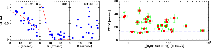
Figure 6: Left: sample of intensity radial profiles illustrating the different cases encountered in the analysis of the 1670 GHz line PACS data: outflow with extended emission (BHR71-R), outflow with compact emission (HH1), and outflow with emission that is too weak to allow a meaningful fit (I04166-B). Blue dots are PACS data and red dashed lines are gaussian fits. Right: comparison between the size (uncorrected for the telescope beam) and intensity of the H₂O-emitting region as determined from the gaussian fits illustrated in the left panel. The star symbols indicate data from maps centered at a YSO position and the horizontal dotted line indicates the telescope FWHM at 1670 GHz ($13^{\prime\prime}$).

Fig. 5 compares the H₂O(1670 GHz) and extinction-corrected IRAC4 intensities for the objects that passed our selection criteria (see Table 3 for numerical values and notes). Although there is a good correlation between the H₂O and IRAC intensities at all IRAC bands, we focus on IRAC4 because its passband includes the lowest H₂ rotational transitions observable by IRAC ($S(4)$ and $S(5)$), and is therefore less sensitive to the small fraction of very hot gas that dominates IRAC1 and IRAC2 observations (Neufeld & Yuan 2008). As can be seen in Fig. 5, there is a reasonable correlation between H₂O(1670 GHz) and extinction-corrected IRAC4 intensities that covers almost two orders of magnitude in range and has a Pearson r-coefficient of 0.98. We approximate this correlation with the simple expression

$$I^{*}[\mathrm{IRAC4}]\;(\mathrm{MJy\leavevmode\nobreak\ sr}^{-1})=0.4\;I[\mathrm{H}_{2}\mathrm{O(1670)}]\;(\mathrm{K\leavevmode\nobreak\ km\leavevmode\nobreak\ s}^{-1}),$$

where $I^{*}$[IRAC4] is the extinction-corrected IRAC4 intensity. This correlation is indicated by the dashed line in the figure, and is closely followed by the objects with best-defined emission peaks in both H₂O and IRAC maps: HH211-B, HH54, and CEPE-B. The two objects that lie significantly above the dashed line in Fig. 5 are N1333I3-B2 and HH46-R, which have poorly defined IRAC4 peaks whose intensity may have been overestimated.

The correlation between H₂O and IRAC4 intensities has a number of implications. It supports the relation between the H₂O and H₂ emission initially inferred from the similarity of their spatial distributions, and shows that outflows located in different clouds and powered by sources of different luminosity share a common ratio between H₂O and H₂ intensities. Since the H₂ emission is generally optically thin and approximately proportional to the H₂ column density (Neufeld & Yuan 2008), the H₂-H₂O correlation suggests that the H₂O emission must have similar properties. If so (and the LVG analysis of Sect.7.1 confirms it), the correlation implies that the emitting gas H₂O abundance must be close to constant over the sample. Calculating the exact value of this abundance requires determining the excitation conditions of H₂O, and for this reason, we defer the discussion to Sect. 8.1, where we analyze the combination of the PACS and HIFI data.

4.3 Angular size of the emitting region

The PACS maps of Fig. 2 illustrate the variety of sizes and distributions seen in the H₂O emission. Despite this variety, a common feature stands out: most maps are compact and present well-defined peaks surrounded by more diffuse emission. Such relatively small emission sizes testify to the rather special conditions needed to produce the H₂O emission, and raise the possibility that beam dilution has affected the appearance of the maps and has decreased artificially the observed intensities. To asses this possibility, we quantify the size of the emitting region in the PACS maps.

Given the large variety of sizes and shapes seen in the maps, any attempt to condense all the spatial information into a single “size” parameter is necessarily an approximation. Our goal in this section, however, is not to characterize in detail any of the individual objects, but to derive a statistical estimate of the water-emission size to assess from it the effect of the PACS finite angular resolution. For this reason, we have chosen the simple approach of fitting a gaussian to the radial profile of emission in each of our PACS images. To do this, we have first determined the emission centroid using all positions having an intensity at least half the value of the map peak (to minimize noise effects). Using this centroid, we have created a radial profile of emission, and we have fitted it with a one-dimensional gaussian using a standard least-squares routine (part of the GILDAS analysis package). A sample of radial profiles and their fits are shown in the left panels of Fig. 6, and the resulting estimates of the emission size and peak intensity are presented in Table 2.

The right panel of Fig. 6 presents our estimated H₂O emission sizes as a function of peak intensity for all 26 sources in the sample whose gaussian fit parameters were determined with S/N larger than 3. The only noticeable trend seen in the plot is a generally smaller size for sources that are centered on a YSO position, and which are represented in the figure by star symbols. Several of these sources present values close to the $13^{\prime\prime}$ PACS FWHM (horizontal dotted line), and are therefore consistent with being unresolved. Apart from this trend, no clear correlation between size and intensity can be seen in the plot, and most points seem to be randomly scattered between $13^{\prime\prime}$ and $40^{\prime\prime}$. The two brightest positions in the diagram correspond to the Cepheus E outflow, and their smaller size may be partly enhanced by the larger distance to this source compared to the others in the sample ($\approx 700$ pc compared to $\approx 300$ pc of most other sources).

Using the 26 points shown in Fig. 6, we estimate a mean FWHM size for the H₂O-emitting region of $24.5^{\prime\prime}$, with an rms of $9^{\prime\prime}$. This rms value most likely reflects a scatter in the true sizes of the sources, as illustrated in Fig. 6, and is not simply a result of deviations from gaussian shape in the radial profiles (although this effect is not negligible). Deconvolving each fitted FWHM by subtracting in quadrature a $13^{\prime\prime}$ gaussian (and assuming zero size if the fit value was smaller than $13^{\prime\prime}$), we estimate a typical intrinsic mean source size of $19.4^{\prime\prime}$ with an rms of $12^{\prime\prime}$. We thus conclude that apart from a handful of point-like sources, mostly associated with YSO positions, the H₂O emission in the outflow gas is slightly but significantly extended compared to the PACS $13^{\prime\prime}$ beam size. As a result, dilution factor corrections to the PACS intensities are not expected to be significant (80% of positions not coincident with a YSO require dilution correction less than 2). Of course, a finite size of the emitting region does not imply the absence of unresolved features in the emission. It means that any compact component must be accompanied by extended emission, and that the integrated intensity inside the PACS map has a larger contribution from the extended emission than from the unresolved feature.

5 HIFI data: velocity information

The $39^{\prime\prime}$-resolution HIFI observations of the 557 GHz H₂O line complement the 1670 GHz PACS data by providing velocity information over a region comparable to the PACS field of view. In this section we analyze the HIFI observations of our outflow sample with emphasis on their statistical properties, and in particular on the information they provide about the velocity properties of the H₂O-emitting gas.

As Fig. 2 shows, there is a large range of line shapes and outflow velocities in the HIFI spectra, indicative of the wide variety of outflows present our sample. The fastest H₂O emission corresponds to the blue lobe of the Cepheus E outflow, with a maximum velocity of 100 km s^-1 with respect to the ambient cloud. Next are the red lobes of the BHR71 and NGC1333-I4 outflows, which have values close to or higher than 40 km s^-1. Such high velocities are comparable to those found by Kristensen et al. (2011) and Kristensen et al. (2012) toward the position of the protostellar sources (although they are significantly lower than those of some H₂O masers in high-mass star-forming regions, e.g., Morris 1976). Together, they attest the resilience of the H₂O molecule, and its likely formation in fast post-shock gas.

5.1 Parameterizing the HIFI spectra

To compare the properties of the H₂O emitting gas in the different outflows of our sample we need to condense the variety of observed line shapes into a small set of parameters. A simple-minded but effective approach is to fit gaussian profiles to the spectra, and to use the fit-derived parameters as first order estimates of the emission properties. To carry out the fits, we first mask all channels in each spectrum that show evidence for contamination by NH₃ or that display hints of self absorption by unrelated cold ambient gas. Then, we fit the blanked spectrum with a gaussian profile, and we inspect the result visually to ensure that the fit is meaningful.

Although a symmetric gaussian profile is not the ideal fit to an outflow spectrum, the two main parameters of the fit, the peak intensity and the line width, provide reasonable estimates of the intensity and velocity spread of the outflow H₂O emission. A test comparison between the integrated intensity under the gaussian fit and a more standard estimate based on the integral of the spectrum using the extreme outflow velocities reveals an agreement better than 10%, which is below the calibration uncertainty of the HIFI data (Sect. 2.2). We thus conclude that the gaussian fit returns a meaningful, zeroth-order characterization of the H₂O emission. The results of this fit are summarized in Table 2.

5.2 Line shapes

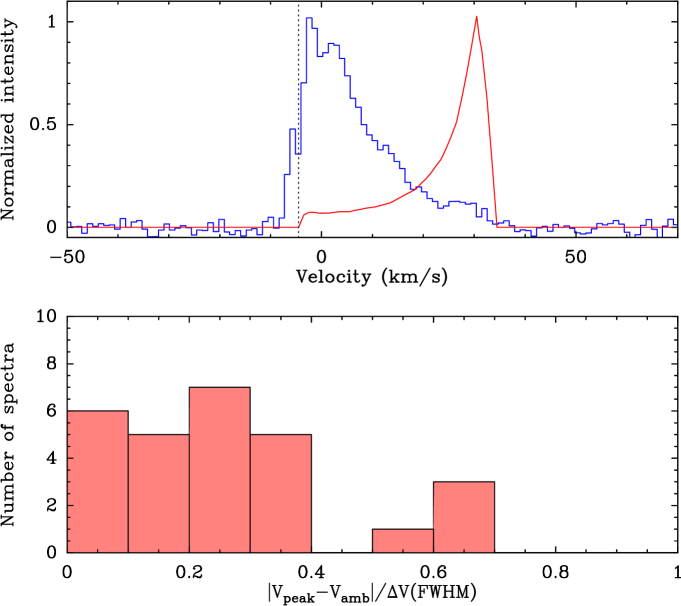
Figure 7: Top: comparison between a representative 557 GHz line profile (BHR71-R, blue histogram and maximum velocity of 40 km s^-1) and a prediction from the planar shock model of Flower & Pineau Des Forêts (2010) (red line, shock velocity of 40 km s^-1 and $n_{H}=2\times 10^{5}$ cm^-3). The vertical dotted line indicates the ambient cloud speed. Note the very different shapes. Bottom: Histogram of the “outflow peak velocity shift” determined from the 557 GHz spectra shown in Fig. 2. The shift corresponding to the planar shock model in the top panel is 4.2 and lies outside the range of observed values.

Although the presence of high-velocity emission is the most noticeable feature of the HIFI spectra, the wing shape of the lines implies that at each outflow position, most of the H₂O-emitting gas has relatively low speeds. This was already seen in the spectra of Fig. 2, and is illustrated in Fig. 7 with the HIFI spectrum toward BHR71-R (blue histogram). The observed wing-like profiles imply that at each outflow position, the amount of gas decreases systematically with velocity, and therefore, that the H₂O emission is dominated by the slowest gas in the outflow. Of course, wing-like profiles are typical of outflow tracers such as CO, but in those species, the outflow contribution can be potentially contaminated with emission from the ambient cloud. The selective nature of H₂O guarantees that the emission arises from warm shocked outflow material (Sect. 6), and indicates that predominance of low-velocity material must be an intrinsic characteristic of the shock-accelerated gas.

The observed wing-dominated H₂O profiles differ significantly from those predicted by the planar-shock models commonly used to interpret H₂O emission. Flower & Pineau Des Forêts (2010), for example, have recently modeled molecular lines observable with the Herschel Space Observatory and generated synthetic spectra of the 557 GHz H₂O line that should be directly comparable with our observations (see their Fig. 8). As illustrated by the red line in the top panel of Fig. 7, these planar-shock model spectra present a narrow component that is approximately centered at the shock velocity and that has a weak wing toward the ambient cloud speed. Such spike-like line profile is almost a mirror image of the observed line profiles and therefore seems inconsistent with our observations.

To quantify the discrepancy between our observations and the predicted model spectra, we have defined a simple parameter that we will refer to as the “outflow peak velocity shift.” This parameter quantifies the effect of the outflow in shifting the velocity of the emission peak in the spectrum, and is equal to the difference in velocity between the H₂O peak and the ambient cloud (determined from N₂H⁺ or NH₃ data and given in Table. 1) divided by the FWHM of the H₂O spectrum. As illustrated by the top panel of Fig. 7, line profiles dominated by wing emission are expected to have outflow peak velocity shifts lower than unity, while spike-dominated spectra are expected to have shifts significantly larger than 1 (the planar-shock model spectrum in the figure has a shift of 4.2).

The bottom panel of Fig. 7 shows a histogram of the outflow peak velocity shifts for the 27 sources in our sample that have peak emission larger than 0.1 K and a meaningful gaussian fit. As expected from the wing-like type of profiles, the histogram is dominated by peak velocity shifts close to zero, and no shift exceeds unity. Many of the small velocity shifts are in fact upper limits, since the self-absorption feature at ambient speeds tends to artificially move the H₂O emission peak away from the ambient cloud velocity. Even without correcting for this effect, the outflow peak velocity shifts in our sample are extremely small, and have a mean value of 0.26 with an rms of 0.19. For comparison, we have estimated outflow velocity shifts for the model spectra of Flower & Pineau Des Forêts (2010) using the examples shown in their Fig. 8. The values lie in the range 2-6 with a mean of approximately 4. Such large values exceed our observed mean shift by more than one order of magnitude, and make the models lie outside the range of velocity shifts covered by the histogram in Fig. 7.

The large discrepancy between observed and model-predicted H₂O line shapes is a strong indication that the plane-parallel shock approximation used by the models is not a good representation of the outflow velocity field. Because of the 1D geometry, the gas in a plane parallel shock cannot escape the compression and piles up at a single velocity downstream, producing a spike-like feature in the spectrum. To avoid this spike and produce the multiplicity of velocities characteristic of a wing-like profile, a more complex velocity field is required. Numerical simulations show that bow-shock acceleration by a precessing or pulsating jet can produce an increase in the range of velocities of the outflow swept-up gas (e.g., Smith et al. 1997; Downes & Cabrit 2003). Models of wide-angle winds interacting with infalling envelopes seem to also produce a significant mix of velocities (Cunningham et al. 2005), although more detailed work is needed to explore the kinematics of this family of solutions. While clearly more complex than planar shocks, these 2D geometries (or alternative, e.g., Bjerkeli et al. 2011) seem necessary to produce the realistic line profiles needed to properly compare models of shock chemistry with outflow observations.

6 Comparison between the 557 GHz, 1670 GHz, and CO(2–1) emissions

6.1 Intensity correlations

In Sect. 4.2 we saw that the 1670 GHz line traces an outflow component similar to that responsible for the H₂ emission, and therefore, hotter than the gas emitting CO(2–1). Now we investigate whether the 557 GHz line traces the same gas component, and therefore arises from hot outflow gas, or traces the colder outflow material responsible for the CO(2–1) emission. To do this, we first need to convolve both the CO(2–1) and 1670 GHz data to the $39^{\prime\prime}$ angular resolution of the HIFI 557 GHz observations so they can be properly compared. Our on-the-fly IRAM 30m CO(2–1) data cover a region $80^{\prime\prime}\times 80^{\prime\prime}$ with Nyquist sampling, so their convolution to $39^{\prime\prime}$ is straightforward. The PACS 1670 GHz data cover a region $47^{\prime\prime}\times 47^{\prime\prime}$ with an array of 25 spectra, and although the coverage is not Nyquist sampled, the data provides enough information to simulate an observation with $39^{\prime\prime}$ resolution. Thus, from now on, our comparisons will use line data that have an equivalent resolution of $39^{\prime\prime}$.

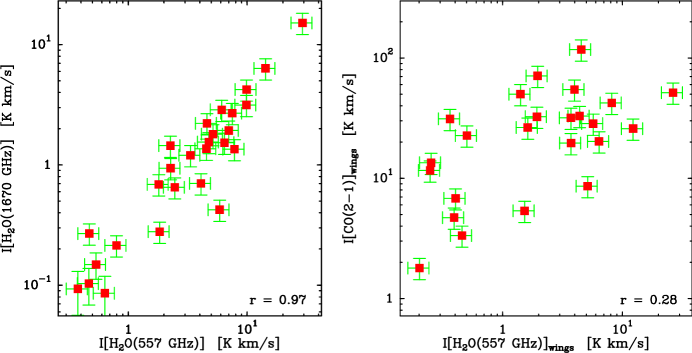
Figure 8: Integrated intensity of the H₂O(557 GHz) line vs H₂O(1670 GHz) (left) and CO(2–1) (right). Note the tighter correlation in the 557-1670 GHz panel that suggests the 557 GHz emission arises from the same gas that emits the 1670 GHz line. The Pearson-r coefficients of each correlation are indicated in the bottom-right corner of the panel.

Fig. 8 presents a comparison between the integrated intensities of the 557 GHz line and those of the 1670 GHz and CO(2–1) lines for all objects in the outflow sample for which the required data are available. The left panel compares the intensities of the 557 GHz and 1670 GHz lines as derived from integrating their intensity over all velocities. Using integrated intensities for the 1670 GHz line is unavoidable due to the lack of effective velocity resolution in the PACS data. For consistency, we have integrated the 557 GHz line profile over all velocities for which the emission was detected, simulating a velocity-unresolved observation. As can be seen, there is a tight correlation between the intensities of the 557 and 1670 GHz lines over the two orders of magnitude covered by our data. The scatter of points with respect to a linear fit (in log scale) is low, and the Pearson’s r coefficient of the dataset is 0.97. This implies that the correlation between the intensities of the 557 and 1670 GHz lines is statistically significant.

In contrast with the correlation between the two H₂O transitions, the right panel of Fig. 8 shows that the 557 GHz and CO(2–1) lines behave almost independent of each other. This right panel presents the 557 GHz and CO(2–1) line intensities with the same logarithmic scale as in the plot of the 557 and 1670 GHz intensities, so the two scatter plots in the figure can be compared directly. To avoid contamination from the bright ambient cloud in the CO(2–1) emission, the intensities shown in the 557 GHz-CO(2–1) scatter plot exclude the contribution from the central 6 km s^-1, which according to an inspection of the spectra is the maximum range of the ambient emission in the objects of our sample. Because of this velocity exclusion, the right panel of Fig. 8 compares intensities in the outflow regime only, and is independent of contributions from ambient cloud emission, absorption, or even contamination from the reference position. As can be seen in Fig. 8, the scatter in the 557 GHz-CO(2–1) plot is higher than in the 557-1670 GHz plot to the left, and the Pearson r-coefficient is only 0.28. This indicates that any correlation between the 557 GHz and CO(2–1) intensities has only a very low statistical significance. (Including the contribution from the ambient cloud regime further degrades the correlation and decreases the r-coefficient.)

The plots in Fig. 8 help answer the question of whether the gas responsible for the 557 GHz line emission resembles the 1670 GHz-emitting gas or the one producing CO(2–1). As can be seen, the 557 GHz intensity is significantly more correlated with the 1670 GHz intensity than with CO(2–1), and this stronger correlation suggests that the 557 GHz-emitting gas is more closely connected to the 1670 GHz-emitting gas than to the gas responsible for the CO(2–1) line. The correlation between the 557 and 1670 GHz intensities is in fact so tight and uniform over the two orders of magnitude in intensity covered by our sample that it seems unavoidable to conclude that the two H₂O lines arise from the same volume of gas.

A common origin of the 557 and 1670 GHz H₂O emissions also helps explain the weak correlation between the 557 GHz and CO(2–1) intensities. In Sect. 4.2, we saw that the 1670 GHz and CO(2–1) emissions are often spatially offset, and that they likely arise from different volumes of outflow gas. Our finding now that the 557 GHz emission arises from the 1670 GHz-emitting gas implies that the 557 GHz emission should also be spatially offset from the CO(2–1) emission, even if the effect cannot be directly resolved with the low angular resolution of the HIFI observations. This different physical origin of the 557 GHz and CO(2–1) emissions seems the likely cause of the only weak correlation between the 557 GHz and CO(2–1) intensities in the scatter plot of Fig. 8.

6.2 Spectral profiles

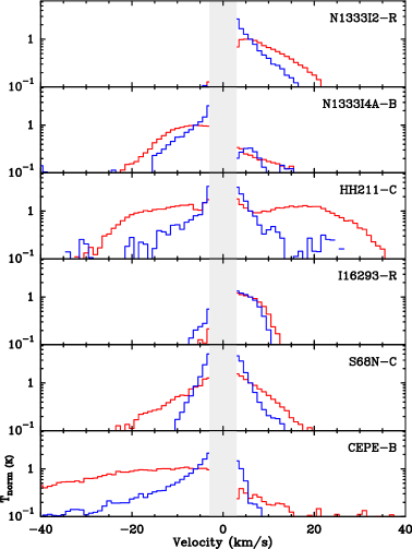
Figure 9: Comparison in log scale between spectra of H₂O(557 GHz) (red) and CO(2–1) (blue) for the six brightest outflows of our sample illustrating the systematicly flatter wings in the H₂O line. For ease of comparison, all spectra have been re-centered at zero velocity, and the intensities have been normalized at an outflow velocity of 6 km s^-1. The central $\pm 3$ km s^-1 part of the spectra have been blanked to avoid contamination from ambient cloud emission.

The velocity information contained in the H₂O and CO spectra offers additional clues on the properties of the gas components responsible for the two emissions. A first comparison between H₂O and CO spectra in outflows was carried out by Franklin et al. (2008), who used 557 GHz data from SWAS and CO(1–0) data from the FCRAO 14m telescope. These data represented emission averages over the full extent of the target outflows due to the low resolution of the SWAS observations, and showed that the H₂O lines systematically had more prominent wings than the CO(1–0) lines. A similar behavior has been found by numerous later studies using different telescopes, spatial resolutions, and (low) $J$ values of the CO line (Bjerkeli et al. 2009; Kristensen et al. 2012; Santangelo et al. 2012; Vasta et al. 2012; Nisini et al. 2013). Kristensen et al. (2012), in particular, used Herschel 557 GHz data toward a sample of 29 YSOs, many of them associated with outflows in our survey, and compared them with JCMT CO(3–2) data convolved to the same angular resolution. They found that the 557 GHz outflow line wings were systematically flatter than the CO(3–2) line wings, and that 557 GHz/CO(3–2) line ratio increased on average by more than one order of magnitude between the lowest and highest speeds in the outflow. Similar 557 GHz/CO(3–2) line ratio increases with velocity have been found by Nisini et al. (2013) toward a number of outflow positions in L1448.

The 557 GHz observations of our survey complement the YSO-centered observations of Kristensen et al. (2012), since most of our positions exclude the central object. For this reason, we have used our survey data to extend the comparison between H₂O and CO spectra, and to search for systematic deviations between the H₂O and CO outflow wing components. While our H₂O data have a lower S/N than the data from Kristensen et al. (2012), the 557 GHz H₂O lines clearly show a pattern of more prominent outflow wings than the CO(2–1) lines, in good agreement with previous studies. Fig. 9 illustrates this pattern with spectra in logarithmic scale from the six brightest objects in our sample. These spectra have been normalized to unity at a velocity of 6 km s^-1 away from the ambient speed to ensure that the wing comparison is not affected by ambient cloud emission (which we estimate extends only $\pm 3$ km s^-1 from the systemic velocity). As can be seen, the H₂O wings (in red) are significantly flatter than the CO(2–1) wings (in blue) at all outflow velocities larger than 6 km s^-1. While this pattern is general, the difference between the H₂O and CO wing slopes depends on the object, being smallest toward I16293-R and being highest toward HH211-C and CEPE-B. Our survey data, and additional lower intensity data not shown here, suggest that the difference between the H₂O and CO outflow slopes may increase as the the H₂O linewidth of the spectrum increases, although higher S/N data are needed to put this trend on solid ground.

Franklin et al. (2008) interpreted the flatter H₂O line wings and the increase in the H₂O/CO ratio with velocity as an indication of an increase in the H₂O abundance toward the fastest outflow gas. This interpretation, however, assumed that both the H₂O and CO emissions arise from the same material, and that the ratio between the H₂O and CO intensities is proportional to the ratio between column densities. As discussed before, a number of Herschel observations indicate that the H₂O and low-$J$ CO emissions originate in different gas components, and therefore, that the ratio between the H₂O and CO intensities does not correspond to a ratio between column densities in the same volume of gas (Santangelo et al. 2012; Nisini et al. 2013). For this reason, the latter H₂O line wings and the increase in the H₂O/CO ratio with velocity cannot be interpreted as an abundance effect. It is more likely that it results from the H₂O-emitting component having a significantly larger fraction of fast-moving gas than the CO(2–1)-emitting gas. This difference could result from the H₂O-emitting gas representing material that has suffered a faster shock than the CO-emitting gas, or alternatively, it could indicate a time evolution effect, by which the H₂O-emitting gas represents recently-shocked material that with time will evolve into the colder and slower CO-emitting component. More detailed observations involving additional transitions of both H₂O and CO are needed to clarify this issue.

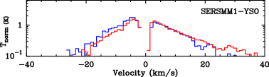
Figure 10: Comparison between H₂O 557 (red) and 1670 GHz (blue) spectra in log scale toward the SERSMM1 YSO illustrating their similar outflow wing slopes. The spectra has been re-centered in velocity and normalized in intensity as those in Fig. 9. (Data to be presented in Mottram et al. 2013.)

If the different physical origin of the 557 GHz and CO(2–1) emissions is associated with a difference in the slope of their line profiles, the common origin of the 557 and 1670 GHz emissions suggests that the two lines should have similar profiles. As mentioned above, our PACS 1670 GHz data do not resolve the emission in velocity, so they cannot provide information on the shape of the spectral profiles. Several sub-projects within WISH, however, have carried out HIFI observations of the 1670 GHz line toward a number of outflow sources, and these data provide a limited sample to compare 557 and 1670 GHz line profiles. Santangelo et al. (2012) and Vasta et al. (2012), for example, carried out multi-line analysis of selected positions in the L1448 and L1157 outflows, and their data show that the 557 and 1670 GHz line profiles are more similar to each other than to the low-$J$ transitions of CO, even when observed with telescope beams that differ by a factor of 9 in area. Additional velocity-resolved observations of the 557 and 1670 GHz lines will be presented by Mottram et al. (2013), who observed five low-mass YSOs, three of them powering outflows included in our survey. While the Mottram et al. (2013) observations are centered on the YSO position, and therefore do not sample the same outflow gas represented in the 557-1670 GHz intensity correlation of Fig. 8, they are the closest data set with which we can check the expected similarity between the 557 and 1670 GHz line profiles in our outflow sample. As Mottram et al. (2013) show, the 557 and 1670 GHz line profiles do in fact look extremely similar. To illustrate it, we present in Fig. 10 a superposition between the 557 and 1670 GHz spectra from SERSMM1, the brightest source that is common to our sample and that of Mottram et al. (2013). The spectra in the figure have been normalized and presented as those in Fig. 9, to allow a direct comparison. As can be seen, the two H₂O lines present almost equal wing slopes, despite having been observed with telescope beams that differ by a factor 9 in area. This good match between the two H₂O spectra represents a strong confirmation that the two transitions must originate from the same gas component.

6.3 The I(557)/I(1670) intensity ratio

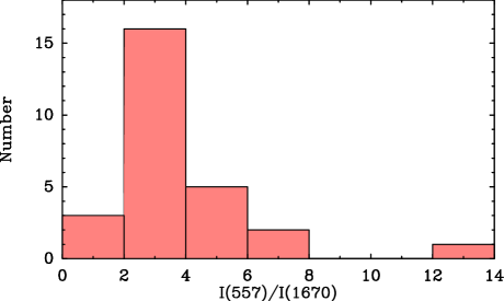
Figure 11: Histogram of the intensity ratio between the H₂O 557 and 1670 GHz lines. Note the narrow peak between values 2 and 4 that contains 60% of the sample.

An alternative measure of the tight correlation between the 557 and 1670 GHz intensities comes from the distribution of the $I(557)/I(1670)$ ratio. This ratio is more robust than the individual intensities, since it is less sensitive to beam dilution and the impact of the ambient self absorption, assuming that the absorption affects the two lines in a similar way (as suggested by the data from Mottram et al. 2013). For this reason, the $I(557)/I(1670)$ ratio is a better tool to constraint the physical conditions of the emitting gas, an issue which will be explored further in Sect. 7.2, where its value is connected to the gas thermal pressure.

Fig. 11 shows a histogram of the $I(557)/I(1670)$ ratio in our outflow sample. As can be seen, the histogram presents a narrow distribution, with 60% of the objects having ratios between 2 and 4. This narrow distribution of ratios is a direct consequence of the tight correlation between the two intensities seen in Fig. 8, and makes the $I(557)/I(1670)$ ratio one of the main observables from our outflow survey.

An important property of the $I(557)/I(1670)$ ratio is that it has a simple interpretation in terms of line excitation. In the next section, we will use an LVG radiative transfer analysis to show that both the 557 and 1670 GHz lines are close to the optically thin limit. In this limit the ratio can be written as

$${I(557)\over I(1670)}={1\over 3}\;e^{53.4/T_{\mathrm{e}x}(2_{12}-1_{10})},$$

where $T_{\mathrm{e}x}(2_{12}-1_{10})$ is the excitation temperature in kelvins between the upper levels of the 1670 and 557 GHz transitions (the cosmic background radiation has been ignored due to the high frequencies of the lines and the high temperature of the gas).

While $T_{\mathrm{e}x}(2_{12}-1_{10})$ is not a good approximation of the gas kinetic temperature due to the strong subthermal excitation of the H₂O molecule, the LVG analysis shows that $T_{\mathrm{e}x}(2_{12}-1_{10})$ is a good approximation to the excitation temperature of the 557 and 1670 GHz transitions for the typical conditions in our sample. Using the previous formula, we estimate a mean (and median) $T_{\mathrm{e}x}(2_{12}-1_{10})$ value of 24 K, and an rms of 5 K. The small dispersion of $T_{\mathrm{e}x}(2_{12}-1_{10})$ distribution shows that despite our water lines covering two orders of magnitude in intensity, the emission originates from a relatively narrow range of physical conditions. Determining such conditions in terms of density and temperature is the goal of the next section.

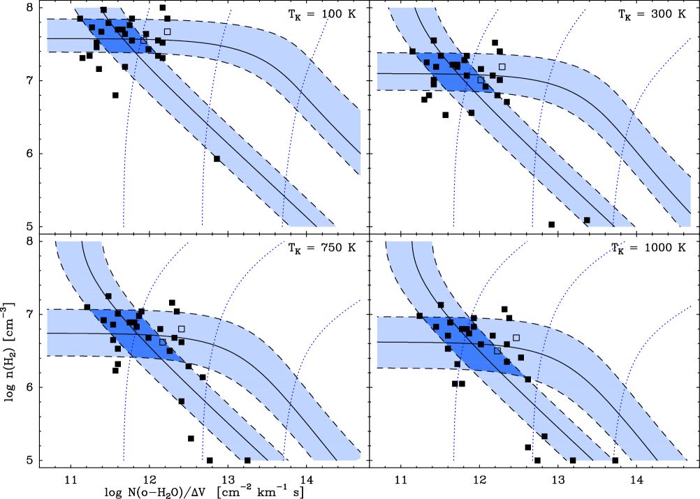
Figure 12: LVG results from the combined analysis of the 557 and 1670 GHz H₂O lines. Each panel corresponds to the choice of gas kinetic temperature indicated in the upper right corner. The filled squares represent the best fit values of $n({\mathrm{H_{2}}})$ and $N(\mathrm{H_{2}O})/\Delta V$ for the outflows in our sample (one point per source), and the open squares represent fits for L1157-B1 (rightmost point) and L1448-R4 derived using literature values. In all cases, the $n({\mathrm{H_{2}}})$ and $N(\mathrm{H_{2}O})/\Delta V$ values have been determined by finding, among a grid of more than $10^{4}$ LVG models, the one that best fits the observed $I(557)/I(1670)$ ratio (within $39^{\prime\prime}$) and the peak $I(1670)$ intensity (within $13^{\prime\prime}$). As discussed in the text, this method extrapolates the $I(557)/I(1670)$ ratio to a resolution of $13^{\prime\prime}$ based on its approximately constant value over the sample. The partially horizontal blue-shaded band is the locus of $I(557)/I(1670)$ values typical of the sample shown in Fig. 11 (the solid line corresponds to a ratio of 3 and the dashed lines to ratios 2 and 4). The blue-shaded band that runs approximately in diagonal is the locus between the first and third quartiles of the observed 1670 GHz peak intensities (solid line is 0.26 K and dashed lines are 0.12 and 0.47 K). The blue dotted lines mark the curves of $\tau(1670)=0.1,1,$ and 10 ordered by increasing $N(\mathrm{H_{2}O})/\Delta V$. The values at the lowest end of the $n({\mathrm{H_{2}}})$ range are upper limits.

7 Physical conditions of the H₂O-emitting gas

7.1 LVG analysis of the H₂O emission

To determine the physical conditions of the gas responsible for the H₂O emission, we need to solve the coupled equations of radiative transfer and statistical equilibrium for the H₂O molecule. To do that, our observations only provide two constraints (the intensities of the 557 and 1670 GHz lines), and this limits our search for solutions to those having homogeneous gas conditions. In reality, the H₂O-emitting gas will likely have internal gradients of density and temperature, so our modeling should be considered as providing average values of the real gas conditions.

The large range of velocities present in the HIFI spectra indicates that the emitting gas contains strong velocity gradients. These gradients decouple the radiation from different positions of the cloud, and justify using the so-called large velocity gradient (LVG) limit to solve the radiative transfer. In this limit, the radiative excitation term of the statistical equilibrium equations can be treated locally, and this simplifies enormously the solution (Sobolev 1960; Castor 1970; Scoville & Solomon 1974; Goldreich & Kwan 1974).

Our LVG code is based on that presented by Bieging & Tafalla (1993), and assumes that the emitting gas is spherical, since spherical geometry provides a solution that is intermediate among the possible choices of geometry and line broadening mechanism (White 1977). To include the H₂O molecule in the code, we have added the molecular parameters provided by the Leiden Atomic and Molecular Database (LAMDA, Schöier et al. 2005), which include the most recent collision rates between H₂O and H₂ (Dubernet et al. 2006a, b, 2009; Daniel et al. 2011, 2010; Valiron et al. 2008).

Even using an LVG approximation and assuming homogeneous gas conditions, three parameters are required to specify the solution: the gas kinetic temperature $T_{\mathrm{k}}$, the volume density $n({\mathrm{H_{2}}})$, and the ratio of the H₂O column density over the linewidth, $N(\mathrm{H_{2}O})/\Delta V$. This number of free parameters is larger than the number of our constraints, so the radiative transfer solution is not completely constrained by the data. Thus, to explore the full set of possible solutions, we have run a series of LVG models fixing each time the gas kinetic temperature and varying both $n({\mathrm{H_{2}}})$ and $N(\mathrm{H_{2}O})/\Delta V$ with logarithmic size steps. Each of these constant-temperature grids provides a well-constrained problem in which the intensities of the two H₂O lines can be inverted to derive best-fit values of $n({\mathrm{H_{2}}})$ and $N(\mathrm{H_{2}O})/\Delta V$. This procedure is illustrated in Fig. 12, where we present the results for 4 different grids of kinetic temperature that range from 100 to 1000 K. The 100 K lower limit has been set because colder models predict densities $\ga 10^{8}$ cm^-3, which seem too high for typical outflow gas. Temperatures higher than our 1000 K upper limit are possible, although they exceed typical single-temperature estimates based on H₂ emission data (e.g., Maret et al. 2009), and therefore seem unlikely. In addition to the outflows of our survey (solid squares), we present in Fig. 12 the results for two well-known outflow positions whose H₂O emission has been studied previously, L1157-B1 and L1448-R4 (open squares). To obtain these solutions, we have used the intensities and line ratios provided by Lefloch et al. (2010), Nisini et al. (2010a), Santangelo et al. (2012), and Nisini et al. (2013), and we have performed the same radiative transfer analysis applied to the outflows in our sample. The overlap between all solutions shows that our survey outflows are not qualitatively different from those of the two prototypical L1157 and L1448 systems.

As can be seen in Fig. 12, most best-fit points in each constant-temperature grid cluster inside a narrow range of $n({\mathrm{H_{2}}})$ values, especially for the lowest choices of $T_{\mathrm{k}}$. This clustering of solutions is a direct consequence of the narrow range of $I(557)/I(1670)$ ratios found in the previous section. To better appreciate this effect, we have plotted in each panel several lines of constant $I(557)/I(1670)$ ratio, using as before values convolved to a $39^{\prime\prime}$ resolution. These lines run almost horizontally for low values of $N(\mathrm{H_{2}O})/\Delta V$ because in this optically thin regime the excitation is controlled by collisions and therefore is fixed for each $n({\mathrm{H_{2}}})$. In the optically thick regime (large $N(\mathrm{H_{2}O})/\Delta V$), the lines of constant ratio bend down toward lower $n({\mathrm{H_{2}}})$ values because the contribution from photon trapping lowers the density required to achieve a given excitation.

As can be seen in the figure, most outflow points lie inside the horizontal blue band bounded by line ratios 2 and 4 (dashed lines), which has a width of 0.5-0.6 dex in density. This means that most solutions deviate less than a factor of 2 from the density corresponding to the median ratio of 3 (solid line). Although the horizontal blue band contains most of the LVG points, a number of solutions lie at significant lower densities. These points correspond to $I(557)/I(1670)$ ratios that exceed 4, and their large spread in the plot reflects the strong sensitivity of the derived gas density to the value of the line ratio when it is larger than 4.

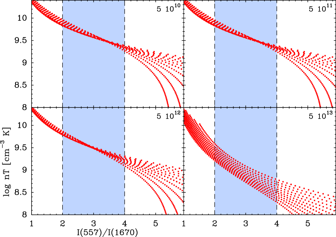
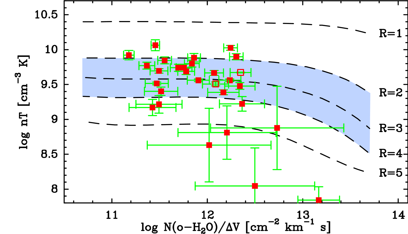
Figure 13: Left: gas thermal pressure $nT$ vs. $I(557)/I(1670)$ as determined by a series of LVG models. Each panel summarizes the result from more than 1000 LVG models of different density and temperature (see text), together with a constant value of $N(\mathrm{H_{2}O})/\Delta V$ indicated in the upper right corner (units are cm^-2km^-1s). The blue-shaded region marks the interval of ratios between 2 and 4 that contains 60% of the outflow sample. Right: Thermal pressure $nT$ vs. $N(\mathrm{H_{2}O})/\Delta V$ for the outflows in our sample. Each point represents an outflow (open squares correspond to L1157-B1 and L1148-R4), and the mean values and error bars have been determined from the LVG results shown in Fig. 12. The dashed lines labeled with $R$ ($=I(557)/I(1670)$) have been derived from the models in the left panels. Again, the region between $R$ values of 2 and 4 is shaded in blue.

While the value of the $I(557)/I(1670)$ ratio controls the best-fit volume density in the LVG model, the absolute line intensities control the derived value of $N(\mathrm{H_{2}O})/\Delta V$. This is illustrated in Fig. 12 by the lines of constant 1670 GHz intensity. These lines cross the LVG grid diagonally from top to bottom, and tend to run almost vertically at high densities, since the levels are thermalized. In the optically thin regime (low $N(\mathrm{H_{2}O})/\Delta V$) the constant-intensity lines intersect the curves of constant $I(557)/I(1670)$ ratio at a single point, and this means that for a given line ratio, different I(1670) intensities correspond to solutions of fixed $n({\mathrm{H_{2}}})$ but different $N(\mathrm{H_{2}O})/\Delta V$.

If the column density estimate depends sensitively on the observed line intensity, our results are potentially sensitive to beam-dilution effects. In Sect. 4.3 we saw that the PACS maps indicate typical emission sizes of $20^{\prime\prime}$, which is significantly smaller than the HIFI $39^{\prime\prime}$ resolution used estimate the $I(557)/I(1670)$ ratio. For this reason, an LVG analysis using $39^{\prime\prime}$-beam intensities will necessarily underestimate the value of $N(\mathrm{H_{2}O})$. To mitigate this problem, we have carried out our LVG analysis with the unconvolved 1670 GHz intensities, which have an intrinsic resolution of $13^{\prime\prime}$ and are unlikely to be strongly beam diluted (Sect. 4.3). In addition, for each source we have chosen the peak value of the 1670 GHz line, which maximizes the H₂O column density estimate. Of course, self-consistency requires that we also use 557 GHz line intensities with $13^{\prime\prime}$ resolution, instead of the $39^{\prime\prime}$ HIFI beam. As no high-resolution data exist, we have assumed that the $I(557)/I(1670)$ ratio in the $13^{\prime\prime}$ PACS beam is the same as in the $39^{\prime\prime}$ beam. This assumption is supported by the almost constant value of the line ratio in the sample, which suggests that the ratio is independent on the source distance and on how well centered on the emission peak our 557 GHz observations were, and therefore, that it varies little inside the mapped region. Thus, our LVG analysis can be thought as constrained by two independent measurements: the $I(557)/I(1670)$ ratio determined with a $39^{\prime\prime}$ beam and extrapolated to $13^{\prime\prime}$, and the intensity of the 1670 GHz line truly measured with $13^{\prime\prime}$ resolution.

As Fig. 12 shows, typical $N(\mathrm{H_{2}O})/\Delta V$ values in our sample are around 10¹² cm^-2 km^-1 s, with few points exceeding 10¹³ cm^-2 km^-1 s. These values represent the peak column density for each source, since they were estimated using the peak 1670 GHz intensity. Other positions of each source lie horizontally to the left in the LVG diagrams because they have the same line ratio (assumed constant in each source) and a lower 1670 GHz intensity. The relatively low $N(\mathrm{H_{2}O})/\Delta V$ values we derive reinforce the idea that the H₂O emission cannot be optically thick. Indeed, the lines of constant $\tau(1670)$ in Fig. 12 (blue dotted lines) indicate that most points have values below 1, and that moving those points into the optically thick regime would require multiplying most peak intensities by factors of 5-10. This factor seems larger than expected from dilution effects given the source sizes estimated in Sect. 4.3

7.2 The 557/1670 ratio and the gas thermal pressure

The LVG analysis illustrates how our observations cannot constrain completely the physical conditions of the H₂O-emitting gas. The data can be fitted with a solution where the gas has a relatively low temperature (100 K) together with a high density ($\approx 4\times 10^{7}$ cm^-3), or has a higher temperature (1000 K) and a lower density ($\approx 4\times 10^{6}$ cm^-3). Both extreme solutions, and many other in between, produce the same level of excitation consistent with the observed $I(557)/I(1670)$ ratio.

The opposite role that density and temperature play in the LVG solution suggests that their product can be determined better than each individual quantity. This $n(\mathrm{H}_{2})T_{k}$ product ($nT$ hereafter) corresponds to the thermal pressure of the gas ($P/k$), and is a useful parameter to constrain shock models. To explore how well it can be determined from our data, we have run series of more than 1000 LVG models fixing each time the column density and covering with a fine grid both the density ($10^{5}$ to $10^{8}$ cm^-3 with logarithmic step of 0.03) and the temperature (100 to 1000 K with a logarithmic step of 0.1). For each model, the derived intensity of the 557 and 1670 GHz lines has been used to estimate the $I(557)/I(1670)$ ratio, and scatter plots of $nT$ vs $I(557)/I(1670)$ are presented in the left panel of Fig.13 for four different column density values. As can be seen, there is a tight correlation between $nT$ and $I(557)/I(1670)$ when the line ratio is lower than 5 and $N(\mathrm{H_{2}O})/\Delta V<5\times 10^{13}$ cm^-2 km^-1 s, which are conditions typical of the outflow data. This means that the observed line ratio can be used to constrain the gas pressure, even if we cannot distinguish between the high and low temperature solutions in the LVG analysis.

To determine the gas pressure in each object of our sample, we have used the four LVG solutions shown in Fig. 12 and estimated the mean and dispersion values of $nT$ and $N(\mathrm{H_{2}O})/\Delta V$. The results are summarized in Table 2 and plotted in the right panel of Fig. 13. As expected, the dispersion in $nT$ is relatively small for line ratios $R<5$ ($<0.2$ dex), which include 75% of our sample. Typical $nT$ values exceed $10^{9}$ cm^-3 K, and the pressure corresponding to points with $R=3$ (the median line ratio of our sample) and typical H₂O column densities is $4\times 10^{9}$ cm^-3 K.

The high gas pressures derived with our analysis are consistent with the idea that the H₂O-emitting gas has been compressed by a strong shock. To determine the nature of such a shock, we first estimate the pressure increase with respect to pre-shock conditions. Since most of our outflow positions lie at some distance from the driving YSO, we assume pre-shock densities and temperatures typical of the cloud gas that surrounds the dense cores, which means $T=10$ K and $n=10^{4}-10^{5}$ cm^-3 (e.g., Bergin & Tafalla 2007). These values imply that the pre-shock pressures were in the range $10^{5}-10^{6}$ cm^-3 K, and therefore, that the pressure enhancement by the shock has been on the order of $10^{4}$.

A pressure enhancement of $10^{4}$ seems uncomfortably high for a number of shock models, especially those of C type. In these shocks, the gas compression is significantly limited by the contribution from the magnetic field, and this leads to a relatively small gas pressure jump. This can be seen in Fig. 1 of Flower & Pineau Des Forêts (2010), that provides detailed density and temperature profiles for a number of C-shock models. By simply multiplying the density and temperature values in these profiles, we estimate that the gas pressure jump in C-type shocks is not expected to exceed a value of 500 even for shock velocities of 40 km s^-1 (the highest considered by the authors). Pressure jumps for shock velocities of 20 km s^-1, which are closer to the total velocity extent we find in the H₂O lines, are typically on the order of 200, which is much smaller than the $10^{4}$ factor we derive from the observations. C-type shock models seem therefore inconsistent with the observed pressure jumps determined from the H₂O data.

J-type shocks, where a weak magnetic field plays no dominant role in the kinematics, provide a better alternative to explain the observed pressure jumps. Simple analysis of these shocks using the Rankine-Hugoniot jump conditions shows that for high velocities, the post-shock over pre-shock pressure ratio is proportional to the Mach number squared (e.g., Shu 1992). A shock velocity of 20 km s^-1 corresponds approximately to a Mach number of 100 for 10 K gas, so the expected initial to final pressure ratio in this type of J-shock is about $10^{4}$, similar to what we derive from the observations. The more detailed shock models presented by Flower & Pineau Des Forêts (2010) (bottom panels of their Fig. 1), confirm the simple analytic theory, and show pressure jumps close to $10^{4}$ for a shock speed of 20 km s^-1 and pre-shock H₂ densities of either $10^{4}$ or $10^{5}$ cm^-3. The high pressure jumps derived by our analysis, therefore, strongly favor J-type shocks over C-type shocks as the type of disturbance responsible for the physical conditions of the H₂O-emitting gas in outflows. If the H₂O component coexists with the H₂ gas responsible for emission seen in the Spitzer IRAC images (as suggested in Sect. 4.2), our results imply that J-type shocks must also be responsible for the H₂ emission seen at near and mid IR wavelengths (see also Nisini et al. 2010b).

8 H₂O abundance in the outflow gas

8.1 H₂O abundance in the warm outflow component

The abundance of H₂O in the shocked outflow gas is a critical parameter to test chemical models. Over the years, a number of authors have estimated the abundance of H₂O in low-mass outflows using data from different telescopes, such as ISO, SWAS, Odin, and Herschel (e.g., Liseau et al. 1996; Nisini et al. 1999; Giannini et al. 2001; Franklin et al. 2008; Bjerkeli et al. 2009; Lefloch et al. 2010; Kristensen et al. 2011; Vasta et al. 2012; Santangelo et al. 2012; Nisini et al. 2013). Unfortunately, the derived values cover a very wide range, from about $10^{-7}$ to $10^{-5}$, and no consensus exists on what the “typical” H₂O abundance in an outflow is.

It is possible that the large range of H₂O abundances arises from true chemical differences between the outflows, or from differences in the abundance of the various temperature components in the shocked gas. Still, a significant part of the dispersion seems to result from differences in the analysis used to derive the abundance. Broadly speaking, two main issues have contributed to the multiplicity of H₂O abundance estimates. On the one hand, some estimates have used low-$J$ transitions of CO to infer the H₂ outflow column density from which the H₂O abundance is determined, while other estimates have used direct determinations of the H₂ column density from emission at near or mid IR wavelengths. As discussed in Sects. 4.1 and 6.2, the low-$J$ transitions of CO trace a cold outflow component than does not coexist with the H₂O-emitting gas, and as a result, H₂O abundance determinations based on low-$J$ CO data are likely to be in error. The mid-IR H₂ emission, on the other hand, seems closely-connected with the H₂O-emitting gas (Sect. 4.1), and therefore represents a more reliable tracer of the outflow column density responsible for H₂O. In this section, we will therefore use this mid-IR H₂ emission as the reference for the H₂O-abundance determination (see Vasta et al. 2012 and Santangelo et al. 2012 for a similar approach).

The other cause for the dispersion of H₂O abundance values in the literature is the diversity of radiative transfer solutions proposed from the H₂O emission. Large H₂O abundance values tend to be associated with optically thick solutions that infer large H₂O column densities, while low abundance estimates result from solutions where the optical depth of the H₂O emission is low or moderate (see Kristensen et al. 2011 for a comparison between the two different approaches in the case of the L1448 outflow). As discussed above (7.1), our LVG analysis suggests that the H₂O emission from the outflows in our sample is optically thin or has at most moderate optical depth. This means that our H₂O abundance estimate is expected to favor values near the low end of the published range.

If the H₂O emission has at most moderate optical depth, the intensity of the 1670 GHz line from any object must be proportional to the column density of its emitting H₂O. This means that the linear relation between $I(1670)$ and IRAC4 intensities found in Sect. 4.2 (and illustrated in Fig. 5) must translate into a similar relation between H₂O and H₂ column densities. From this relation, it should be possible to derive an H₂O abundance value that is representative of our outflow sample. Of course, the $I(1670)$ vs IRAC4 correlation has significant scatter, and our radiative transfer analysis has a number of uncertainties. This allows for some scatter in the H₂O abundance of the different outflows. Still, the scale of this scatter should be on the order of a factor of a few, and not the two orders of magnitude seen in the literature.

Before proceeding with the analysis, it is important to check the consistency between the treatments of the H₂O and H₂ emission. H₂ radiative transfer solutions often result in low density estimates, as illustrated by the less than $10^{4}$ cm^-3 values derived by Neufeld et al. (2009) from Spitzer observations. This is of course much lower than our $>10^{6}$ cm^-3 estimate from the H₂O observations, and brings into question whether the H₂O and H₂ emissions can be reproduced with the same physical conditions (a necessary requirement if the emissions coexist). That this is the case has been recently shown by the Giannini et al. (2011), who have re-analyzed the same H₂ rotation lines studied by Neufeld et al. (2009), but this time complementing them with vibrational transitions. This new analysis has increased the original density estimate of the H₂-emitting gas to values consistent with those derived from our H₂O analysis, showing that it is possible to interpret both emissions with a consistent set of gas conditions.

If the H₂O and H₂ emissions arise from the same volume of gas, to calculate an outflow-wide estimate of the H₂O abundance we need to calculate the proportionality factors between the $I(1670)$ and IRAC4 intensities and the corresponding H₂O and H₂ column densities. As a first step, we derive the conversion factor between the IRAC4 intensity and the H₂ column density. We do so following the methodology of Neufeld & Yuan (2008), who have shown that IRAC observations of shocked gas can be reproduced assuming that the emitting material has a distribution of column densities that depends on temperature as a power law with the form $T^{-\beta}$. The $\beta$ parameter is typically 4 for bipolar outflows, and the power law distribution seems valid approximately between 300 and 4000 K (Nisini et al. 2010b; Giannini et al. 2011). Our analysis of the IRAC4 emissions makes therefore use of these literature values, together with a gas density of $5\times 10^{6}$ cm^-3 (Giannini et al. 2011) and an ortho-to-para ratio of 2.2 for H₂ (Nisini et al. 2010b), and predicts the emission of the different H₂ rotation lines for temperatures between 300 and 4000 K. For this we have used the LVG code, this time with the H₂-H₂ collision rates from Flower & Roueff (1999) (as provided by the BASECOL database, see Dubernet et al. 2006b) and the Einstein A coefficients for H₂ from Wolniewicz et al. (1998). By integrating the contribution from all temperatures, and assuming that the $S$(4) and $S$(5) transitions contribute to the IRAC4 intensity with the weights determined by Neufeld & Yuan (2008), we have calculated a relation between H₂ column density and IRAC4 intensity with the form

$$N(\mathrm{H}_{2})\;[\mathrm{cm}^{-2}]=4.5\times 10^{19}\;I^{*}(IRAC4)\;[\mathrm{MJy\leavevmode\nobreak\ sr}^{-1}]$$

where, as in Sect. 4.2, $I^{*}$(IRAC4) is the extinction corrected IRAC4 intensity. To test this relation, we have applied it to the red lobe of L1448 and the blue lobe of BHR71, for which more accurate determinations have been presented by Giannini et al. (2011). Reading the color scale in Figs. 4 and 5 from these authors, we estimate that our analytic N(H₂) estimates agree with the more accurate values within 20%.

While the above column-density-intensity relation is valid for a mix of gas with temperatures between 300 to 4000 K, a single-temperature analysis of the H₂ emission shows that it is equivalent to the relation for isothermal gas at about 600 K. This suggests, that the IRAC4 emission is dominated by the low end of the temperature distribution, which should not be surprising given the steep temperature dependence of the column density implied by the $\beta=4$ exponent.

To calculate now the conversion factor between the 1670 GHz line intensity and the H₂O column density, we need an analysis that is consistent with that of H₂. This means that we cannot apply the single-temperature treatment used in Sect. 7.1, but that we have to assume a distribution of H₂O column densities that also follows a $T^{-\beta}$ law with $\beta=4$. Also, we have to assume the same gas volume density of $5\times 10^{6}$ cm^-3 that was used for H₂. With these values, plus an H₂O ortho-to-para ratio of 3 (e.g., Herczeg et al. 2012), we have run a series of LVG models covering the temperature range from 300 to 4000 K, and we have integrated the resulting intensity of the 1670 GHz line weighting it by the temperature-dependent column density distribution. The resulting relation has the form

$$N(\mathrm{H_{2}O})\;[\mathrm{cm}^{-2}]=4.8\times 10^{12}\;I(\mathrm{1670\leavevmode\nobreak\ GHz})\;[\mathrm{K\leavevmode\nobreak\ km\leavevmode\nobreak\ s}^{-1}],$$

where the column density refers to the total (ortho + para) value.

If we again compare the multi-temperature relation with a single-temperature analysis, we find that it is equivalent to that of an isothermal gas at about 450 K. This temperature is similar to the 600 K derived from the H₂ analysis, confirming the idea that both emissions are dominated by gas at the low end of the temperature distribution. This should not by surprising given the steep power-law assumed for the distribution of H₂ column density with temperature, which implies that, for example, less than 7% of the gas is at temperatures higher than 750 K. It indicates that the H₂O abundance estimate we are about to derive is dominated by gas at around 500 K.

The single-temperature H₂O estimate also allows a consistency check with the pressure analysis of the previous section. Combining the derived 450 K with the assumed density of $5\times 10^{6}$ cm^-3, we derive a gas pressure $\log(nT)=9.35$, which according to Fig. 13 is again inside the range of observations and corresponds to $I(557)/I(1670)=4$. These numbers show that the multi column density analysis of H₂O is consistent both with the analysis of the H₂ emission and with the analysis of the 557 and 1670 GHz intensities presented in the previous sections.

Combining the above intensity-column density relations for H₂ and H₂O with the IRAC4-$I(1670)$ correlation found in Sect. 4.2, we derive an approximate H₂O abundance of $3\times 10^{-7}$ for the gas responsible of the observed 557 and 1670 GHz emission. This value has an uncertainty level of at least a factor of 2, which corresponds to the 0.3 dex rms level in the H₂O column densities for objects with $R=4$ (Fig. 13). Other sources of uncertainty related to the radiative transfer of H₂O and H₂ are possible and can add to the error budget, but they cannot be easily quantified without the observation of additional H₂O lines. In any case, our estimate clearly favors a relatively low abundance value for H₂O, as expected from the optically thin analysis (and in line with recent estimates for individual outflow sources, like L1157 by Vasta et al. 2012 and VLA1623 by Bjerkeli et al. 2012).

Our low H₂O abundance is in clear conflict with the expectation from C-type shock models, which are often used in the analysis of the H₂O emission from outflows. These models consistently predict H₂O abundances in excess of $10^{-5}$ due to an almost complete conversion of oxygen into H₂O (Kaufman & Neufeld 1996; Flower & Pineau Des Forêts 2010). This value exceeds our derived abundance value by more than one order of magnitude and therefore is excluded by our analysis. As mentioned before, however, C-type shocks seem already inconsistent with the high gas pressure inferred for the H₂O emitting gas, so their failure to match the observed H₂O abundance should not be considered surprising. The alternative J-type shock models have unfortunately received much less attention. Flower & Pineau Des Forêts (2010) showed that these models do in fact predict lower H₂O abundances due to its destruction by collisions with atomic hydrogen, although their Fig. 3 suggests that a large enough abundance decrease only occurs in post-shock gas that is too cold to be consistent with our observations. Additional contribution from UV radiation in fast shocks may help decrease the post-shock abundance of H₂O, according to Neufeld & Dalgarno (1989). Further work on destruction mechanisms of H₂O in shocks is clearly needed to understand the low abundances derived from the data.

8.2 H₂O abundance in the cold outflow component

Throughout the paper, we have distinguished between two outflow components, a relatively cold one traced by the low-$J$ CO transitions and a warmer one traced in H₂. The H₂O emission observed by Herschel arises from the warm outflow component, so the H₂O abundance estimated in the previous section only applies to this higher excitation part of the flow. In this section we investigate how much H₂O can be hidden in the cold component of the outflow, and how the H₂O abundance in this component can be further investigated with observations.

Since no model of the different outflow components exist in the literature, our analysis will use the simplest assumptions consistent with the data. We simplify the outflow gas structure as consisting of two components, one responsible for the low-$J$ CO emission and other responsible for the H₂O emission. For the low-$J$ CO-emitting component, we assume a gas temperature of 30 K and a volume density of $10^{5}$ cm^-3, which are values typically derived from low-$J$ molecular transitions (e.g., Tafalla et al. 2010). For the H₂O-emitting gas, we use the values derived in the previous section, i.e., a representative temperature of 450 K and a density of $5\times 10^{6}$ cm^-3.

As a preliminary check, we make sure that our model is consistent with the idea that the low-$J$ CO emission is dominated by the cold component and that the contribution from the warm gas is negligible. To test this, we first calculate the CO column density of the warm outflow. From our analysis of the HIFI data, we derive a mean linewidth is 16 km s^-1, and assuming that the linewidths of the 557 and 1670 GHz are equal, we estimate a the median 1670 GHz line brightness of 0.3 K. These values, together with the relation from the previous section, imply a typical column density of of warm H₂O of $2.3\times 10^{13}$ cm^-2. If we now assume an H₂O abundance of $3\times 10^{-7}$ (Sect. 8.1) together with a standard CO abundance of $8.5\times 10^{-5}$ (Frerking et al. 1982), we derive that the CO column density in the warm component is $7\times 10^{15}$ cm^-2. For the assumed temperature of 450 K and density of $5\times 10^{6}$ cm^-3, an LVG model predicts that the CO(1–0) and CO(2–1) intensities must be $<0.1$ K. Such intensities are clearly smaller than the $\sim 3$ K observed with the IRAM 30m telescope, in agreement with the expectation that little low-$J$ CO emission comes from the warm outflow gas.

We now investigate the H₂O content of the cold outflow component. First, we derive the H₂ column density of this part of the outflow using our complementary IRAM 30m data, which show typical CO(2–1) intensities of 3 K and typical linewidths of 10 km s^-1. Making use again of the LVG code, this time for a temperature of 30 K and a volume density of $10^{5}$ cm^-3 (together with the previous CO abundance), we estimate that the cold outflow gas has a typical H₂ column density of $2.1\times 10^{20}$ cm^-2 in a $13^{\prime\prime}$ beam.

An observational constraint to the H₂O abundance in the cold outflow is that it should remain undetected in our Herschel observations. We thus explore how much H₂O can remain hidden in the cold gas. As a first guess, we assume an abundance level equal to that found in the warm component ($3\times 10^{-7}$). With this value and the LVG model, we predict intensities of 0.85 K km s^-1 for the 557 GHz line and 0.01 K km s^-1 for the 1670 GHz line. These values can be compared with the results from our Herschel observations summarized in Table 2. As can be seen, the predicted 557 GHz intensity from the cold outflow component is almost 6 times smaller than the mean observed value, while the predicted 1670 GHz intensity is two orders of magnitude lower than observed. These lower-than-observed values indicate that the emission from the cold outflow will be overwhelmed by the emission from the warm component, and therefore likely missed in an observation. As a result, it seems possible to hide an H₂O abundance of $3\times 10^{-7}$ in the cold outflow gas for a significant number of outflows from our sample. (Outflows with weak H₂O emission, such as L1551, likely can only hide lower abundances.)

While the above estimate suggests that it is possible to hide an H₂O abundance level of $3\times 10^{-7}$ in the cold component of some outflows, it seems unlikely that a much higher value can remain undetected. The previous LVG solution for a typical (cold) outflow component predicts an optical depth of 1.1 for both the 557 and 1670 GHz lines. This value, together with the expected low excitation temperature of the two transitions ($\sim 5$ K), indicates that a higher H₂O abundance in the cold gas will cause a noticeable self absorption feature in the spectrum. Such a self absorption should be easily distinguishable from the narrow ambient absorption feature seen in the spectra, since it should appear as a relatively broad, wing-like dip in the spectra of both 557 and 1670 GHz lines.

Our 557 GHz HIFI data do not show evidence for broad self-absorptions in the spectra (Fig. 2), and this suggests that abundance values much larger than $3\times 10^{-7}$ are unlikely for the cold outflow gas in the objects of our sample. Some H₂O-bright outflows, however, do present features that could be indicative of cold H₂O. Vasta et al. (2012) and Santangelo et al. (2012) have shown that in L1157-R and L1448-R4, the spectra from transitions connected with the ground state of both ortho and para-H₂O present a deficit of emission at low velocities compared with the spectra from excited levels. Whether these features result from self-absorption by cold H₂O or from an entirely different process needs to be assessed with detailed multi-transition spectral modeling. Such an investigation can potentially provide additional constrains on the H₂O abundance in the cold outflow gas, and thus help complete the analysis of H₂O in outflows presented here.

9 Summary

We have carried out a survey of H₂O emission toward a sample of mostly young bipolar outflows using the Herschel Space Observatory. This survey was part of the “Water In Star-forming regions with Herschel” (WISH) project, and combined HIFI observations of the 557 GHz line with PACS footprints of the 1670 GHz line toward typically two positions in about 20 outflows. From the analysis of these data, together with complementary CO(1–0) and CO(2–1) observations carried out with the IRAM 30m telescope and archive Spitzer/IRAC data, we have reached the following main conclusions:

1. The spatial distribution of the H₂O emission tends to resemble the distribution of IRAC-derived H₂ emission, while it differs from the distribution of both CO(1–0) and CO(2–1). This dichotomy of distributions suggests that H₂O traces a gas component closely connected with the H₂-emitting gas (at hundreds of kelvins) and distinct from the gas producing the low-$J$ CO emission (at tens of kelvins) (Sect. 4.1).

2. In addition to spatial coincidence, the H₂O and H₂ emissions correlate in intensity. We find an approximately linear correlation between the intensities of the 1670 GHz emission traced with PACS and the H₂-dominated intensities observed by the different Spitzer IRAC bands (Sect. 4.2).

3. The analysis of the PACS footprint maps indicates that the H₂O emission is concentrated but not point-like. It often consists of a combination of bright peaks and extended emission, and the deconvolved typical emission size is around $20^{\prime\prime}$ (Sect. 4.3).

4. Most HIFI 557 GHz spectra present outflow wings together with ambient-speed absorption features. The wing shape of the spectra indicates that while some outflow H₂O emission originates in high velocity gas, most of the emission comes from relatively slow material. Such distribution contrasts with the expectation from plane-parallel shock models, which predict spectra having a narrow emission feature at the highest speeds (Sect. 5.2).

5. There is a tight correlation between the integrated intensities of the 557 and 1670 GHz lines over two orders of magnitude, indicating that the two emissions arise from the same volume of outflow gas. On the other hand, any correlation between the 557 GHz and CO(2–1) integrated intensities is weak at most. This is consistent with the two emissions arising from different components of the outflow gas (Sect. 6.1).

6. In agreement with previous work, we find that the H₂O 557 GHz lines have flatter outflow wings than the low-$J$ CO transitions. We interpret this effect as a consequence of the different kinematic properties of the gas responsible for the two emissions (Sect. 6.2).

7. Combining the analysis of the 557 and 1670 GHz lines, we find a relatively narrow range of intensity ratios, with most objects lying between values 2 and 4. The observed line ratios suggest H₂O excitation temperatures on the order of 25 K (Sect. 6.3).

8. An LVG analysis of the 557 and 1670 GHz lines shows that our set of two transitions is not enough to constrain all the physical conditions of the H₂O-emitting gas. It seems equally possible to fit the data with solutions that are relatively cold (100 K) and dense ($4\times 10^{7}$ cm^-3), solutions that are warm (1000 K) and less dense ($4\times 10^{6}$ cm^-3), and a number of intermediate values. In all cases, the models are consistent with the emission being optically thin (Sect. 7.1).

9. While our data cannot constrain separately the density and temperature of the H₂O-emitting gas, they determine with little dispersion the product, which is proportional to the gas pressure. The pressure values we derive indicate that the H₂O-emitting outflow component is over-pressured with respect to the ambient cloud by factors on the order of $10^{4}$. Such high levels of compression seem inconsistent with C-type shocks, and suggest that J-type shocks are responsible for the observed gas conditions (Sect. 7.2).

10. Combining the observed correlation between PACS and IRAC intensities with the excitation conditions derived from the LVG analysis, we derive a typical H₂O abundance of $3\times 10^{-7}$ for the gas responsible of the observed transitions. While uncertain by a factor of a few, this value is significantly lower than standard abundance predictions from C-type shocks. J-type shock models may be able to fit the observations, although more work on H₂O destruction mechanisms in this type of shocks are still needed (Sect. 8.1).

11. Our derived H₂O abundance corresponds to the warm ($\sim 500$ K) component of the outflow gas. A simple model suggests that a similar abundance level could remain hidden in the cold component of a number of outflows. Further progress investigating the abundance of H₂O in this cold outflow component could be made searching for broad self-absorption components in H₂O spectra (Sect. 8.2).