Percolations on random maps I:
half-plane models
Abstract
We study Bernoulli percolations on random lattices of the half-plane obtained as local limit of uniform planar triangulations or quadrangulations. Using the characteristic spatial Markov property or peeling process [5] of these random lattices we prove a surprisingly simple universal formula for the critical threshold for bond and face percolations on these graphs. Our techniques also permit us to compute off-critical and critical exponents related to percolation clusters such as the volume and the perimeter.
1 Introduction
In this work we study different types of percolations (bond and site on the graph and its dual) on several types of infinite random maps. For the sake of clarity we focus on three kinds of maps: triangulations, two-connected triangulations and quadrangulations, though our method is more general and we shall indicate this at times. We show that the spatial Markov property of the underlying random lattice can be used as in [5] in order to compute the critical threshold for percolation as well as geometric properties of critical and near critical clusters. In order to state our results precisely let us start by introducing rigorously the random lattices which we are working with.
Random infinite lattices.
Recall that a finite planar map (map in short) is a finite connected graph embedded in the two-dimensional sphere seen up to continuous deformations. The last decade has seen the emergence and the development of the mathematical theory of “random planar maps”. A primary goal of this theory is to understand the geometry of large random planar structures.
One fruitful approach consists of defining infinite random maps which are the so-called local limits of random planar maps and studying their properties. This idea has been first introduced in the seminal work of Benjamini & Schramm [10] in the context of planar maps and is also related to works of Aldous on local limits of trees [2]. Let us present this setup. As usual in the context of planar maps, we work with rooted maps, meaning maps with a distinguished oriented edge called the root edge of the map. The origin vertex of the root edge is called the origin or root vertex of the map. Following [10] we define a topology on the set of finite maps: If are two rooted maps, the local distance between and is
where is the maximal radius so that is isomorphic to . Here, is the ball of radius in around the origin, namely the map formed by the edges and vertices of that are at graph distance smaller than or equal to from the origin. The set of finite maps is not complete for this metric and so we shall work in its completion which also includes infinite maps (see [16] for a detailed exposition and references).
In this work, we focus on two specific kinds of planar maps: triangulations (all faces have degree ) and quadrangulations (all faces have degree ). We also split the set of triangulations according to their connectivity properties: A -connected triangulation is just a (connected) triangulation and a -connected triangulation is a triangulation with no cut-vertex. It is easy to see that a triangulation can only fail to be -connected if some vertex has a self loop (an edge whose target and origin vertices are confounded).
In the following, all the quantities referring to or -connected triangulations are denoted with the symbols , and the ones referring to quadrangulations are denoted with the symbol . To make statements that hold simultaneously about various types of maps we shall use ’s to indicate one of those, or possibly some other type of planar map (since our methods work in much greater generality).
We review the now classical construction of the Uniform Infinite Planar Maps as weak local limits w.r.t. of uniform finite maps. Let and for we write for a random variable uniformly distributed over the set of type- maps with vertices. Then we have the following convergence in distribution for
| (1) |
The object is a random infinite rooted planar map called the ( or -connected) Uniform Infinite Planar Triangulation (UIPT) if and the Uniform Infinite Planar Quadrangulation (UIPQ) if . The convergence (1) was established by Angel & Schramm [8] in the triangular case and by Krikun [23] in the quadrangulation case . The UIPQ has also been constructed by other means by Chassaing & Durhuus [14], see also [16]. These random lattices have attracted a great deal of attention in recent years [5, 9, 21, 24, 27]. Their large scale geometry is still a source of intensive research and is tightly connected (see [15]) to the Brownian map — the universal continuous random surface obtained as the scaling limit of properly renormalized random planar maps — studied by Le Gall and by Miermont [26, 29].
An important area of research on the random lattices is to understand the behavior of statistical mechanics models on them. Angel [5] already studied site percolation on the UIPT and in particular proved that the critical percolation threshold is almost surely . In this paper, we extend this analysis to several other types of percolation, including both bond and site on both the map and its plane dual.
We pursue the analysis of percolation on random maps by focusing on half-planar models. These models indeed have an especially useful spatial Markov property which makes the analysis of the percolation process much simpler (see [7] for a study of this property). These pages can thus be seen as a step towards the analysis of percolations on the full-plane UIP, which we do in a subsequent paper [6].
In order to construct these half-plane models we first extend (1) to maps with a boundary: A triangulation (or a quadrangulation) with a boundary is a planar map whose faces are triangles (resp. quadrangles) except the face incident on the right of the distinguished oriented edge which can be of arbitrary degree. This face is called the external face. The perimeter of a map with a boundary is the degree of the external face. In general, the boundary of a map can possess “pinch-points”, that are vertices visited at least twice during the contour of the external face. If the boundary does not have pinch-points we say that the boundary is simple, or that is simple.
In the following, all the maps with a boundary that we consider are simple and a map with simple boundary of perimeter is also called a map of the -gon. For and , we denote by the set of all type- maps of the -gon with inner vertices. Note that since quadrangulations are bi-partite, for odd, hence in the case of quadrangulations we implicitly restrict all statements to even. For , let be a random variable uniformly distributed over the sets . Then we have the following convergences in distribution for the distance :
Extending the previous terminology we call these objects the UIP of the -gon.
The preceding convergences are easy corollaries of the convergences with no boundary (1), proved by conditioning on the root having a suitable neighborhood and removing that neighborhood to get the boundary (see [5, 17] for details).
We can now introduce the main characters of our work: the half-plane UIP. These are obtained as limit of the UIPT (resp. UIPQ) of the -gon as . More precisely, we have the following convergence in distribution for
| (2) |
(As noted, in the case the convergence holds along even values of .) The random infinite planar map is called the half-plane UIPT (resp. UIPQ) which we abbreviate by UIHP. The convergence (2) was established in [4] in the case of triangulations and can be easily adapted to the quadrangulation case. See also [17] for a different construction of via bijective techniques “à la Schaeffer” [30].
Percolation.
Having introduced the random lattices, let us specify the models of percolation that we will discuss. Conditionally on , we consider Bernoulli percolation on the edges, vertices or faces, that is, we color the elements of the map white with probability and black with probability independently from each other, and consider the structure of connected white clusters. If we color the edges, we speak of bond percolation, if we color the vertices we speak of site percolation. Coloring faces yields site percolation on the dual of the map (two faces are adjacent if they share an edge) and will be called “face percolation” in this work.
In the triangular case , site percolation has already been analyzed in [4, 5] where it is proved that . The techniques developed in this paper do not apply to site percolation on general planar maps (other than triangulations) and for example the value of is still unknown. However in the case of bond or face percolation we prove that the critical percolation thresholds are almost surely constant and can be expressed by a universal formula relying on a unique parameter depending on the model. To give their values, we introduce for each model of planar map a quantity . This quantity is well defined and can be computed for fairly general models of planar maps. In the main classes we study we have
| (3) |
Theorem 1 (Percolation thresholds).
For , the critical thresholds for bond and face percolations are almost surely constant and are given by
We prove that in each model considered in Theorem 1, at the critical probability, there is no infinite cluster. We also study the associated dual percolations, which in the case of bond percolation is just bond percolation on the dual lattice (edges in a map are in bijection with edges in the dual map, so bond percolation on a map and on its dual use the same randomness, and are dual to each other) and prove the unsurprising identity
In the case of face percolation, the dual percolation is the same percolation but where faces are declared adjacent if they share a vertex. We call it the face′ percolation; here also .
The universal form of the critical probability thresholds expressed in Theorem 1 in terms of holds in a much larger list of maps than the ones we consider in this work and could be applied, e.g. to pentagulations, general planar maps or planar maps with Boltzmann distribution, see [28]. The only quantity to compute would be the equivalent of defined in Proposition 3. Notice also that and are functions of each other. If an oracle such as a physics conjecture or a self-duality property, etc. furnishes one of the two thresholds then Theorem 1 automatically gives the other.
In relation to [5], one key idea which enables us to treat bond percolation is to keep as much randomness as we can during the exploration process. In other words, even after being discovered in the map, the status of an edge can be kept random until it is necessary for the exploration process to know its color.
Critical exponents.
In contrast with the critical threshold values which depend on the local features of model considered, we also compute a few critical exponents which are not model-depend. The exploration of percolation interfaces in random maps involves random walks with heavy-tailed step distribution in the domain of attraction of a totally asymmetric (spectrally negative) stable law of parameter . Using standard results for heavy-tailed random walks we are able to compute critical exponents related to the perimeter (boundary) and the volume of critical percolations clusters.
For sake of simplicity we restricted our proof to the case of site percolation on triangular lattices but there is no doubt that our methods could be adapted to more general cases and would yield the same critical exponents. We now make our setting precise. In we consider the hull of the cluster of a unique white vertex among a full black boundary. That is, we fill the finite holes in the map created by the cluster. We will consider the volume of that is its number of vertices and its boundary which is the number of vertices of adjacent to . We shall also consider the extended hull which is the hull formed by all the triangles adjacent to . More precisely we are interested in the boundary of this extended hull.
Theorem 2 (Critical exponents).
At the critical percolation threshold , we have the following estimates
Here and later we use the notation to denote that is bounded below and above by some absolute constants. The estimates we get in the proof are significantly more explicit than the above statement. In particular, for and we get lower and upper bounds with only a poly-logarithmic correction, see Section 4. Of course, we expect these asymptotics to hold with no correction to the polynomial term.
As can be seen in the last theorem the perimeter of the hull and the perimeter of the extended hull have completely different exponents: after filling-in the “fjords” created by a percolation cluster we drastically reduces its perimeter. This fact is well-known in the physicist literature and it well understood for site percolation on the regular triangular lattice thanks to the SLE processes.
One motivation for this research is the physics theory of -dimensional quantum gravity. In particular the KPZ relation [22] predicts connections between critical exponents of statistical mechanics models on a regular lattice and on a random lattice: if a set defined in terms of a percolation process on a fixed regular lattice has dimension and and the corresponding set defined in terms of percolation has “dimension” , then the KPZ relation states that
For models other than percolation a similar relation holds, with the coefficients in the quadratic relation given in terms of the so-called central charge associated with the model. While there is some recent progress towards understanding this relation in the work of Duplantier & Sheffield [19], the KPZ relation remains unproved. Our work gives another strong indication that the relation does hold for critical percolation interface and boundary of the hull generated, in other words for SLE6 and SLE8/3. This relation has already been checked for various other sets including e.g. pioneer points of simple random walk [9].
The paper is organized as follows. In Section 2 we present in a unified way some enumeration results on random planar maps and introduce the spatial Markov property as well as the peeling process which are the key ingredients of this work. Section 3 is devoted to identifying the critical threshold parameters presented in Theorem 1. The last section uses classical results on heavy-tailed random walk to get off-critical and critical exponents.
Acknowledgments.
This work was started during overlapping visits of the authors to Microsoft Research in 2010. We thank our hosts for their hospitality. We are also grateful to Igor Kortchemski for sharing ideas and references about discrete stable processes.
2 Peeling process
2.1 A few properties of
The random infinite half-planar maps for were obtained as local limits of uniform -angulations of the -gon with faces by first letting and then sending to infinity. Since the distribution of uniform -angulation of the -gon is invariant under re-rooting along the boundary the same property holds true for . More precisely, has an infinite simple boundary that can be identified with , the root edge being . Then for every , the law of the UIHP re-rooted at the edge is the same as the original distribution of . Because of this invariance we allow ourselves to be imprecise at times about the location of the root edge of .
A less trivial property satisfied by is one-endness: it has been proved in [4] in the triangulation case and in [17] for the quadrangulation case that almost surely has one end (recall that a graph is one-ended if the complement of any finite subgraph contains a unique infinite connected component). Roughly speaking, there is a unique way to infinity in .
However, the foremost property of is the spatial Markov property. The half-planar model has the most simple form of spatial Markov property which, roughly speaking, states that the complement of a simply connected region of that contains the root edge (properly explored) is independent of this region and is distributed according to . This property, also called the domain Markov property in this context, is explored further in [7]. In order to make this statement precise we shall need some enumerative background.
2.2 Enumeration
We gather here several results about enumeration and asymptotic enumeration of planar maps. Recall that for respectively, and for , we denote by the sets of all type or triangulations and the set of quadrangulations of the -gon with inner vertices. The reader should keep in mind that if is odd. By convention the set contains the unique map (with simple boundary) composed of a single oriented edge.
All the results presented here can easily be deduced from the exact formulae for (or the intermediate steps to reach them) and can be found in [20] for , in [25] for and in [13] for . By convention the asymptotics for only apply to even values of .
For and we have the following asymptotics for :
| (4) |
where
The asymptotics (4) in general and the exponent are typical to enumeration of planar maps and hold for many other classes of planar maps. As in previous works and as we will see below, the exponent plays a crucial role in the large scale structure of the random lattices. Furthermore, the functions also have a universal asymptotic behavior:
| (5) |
where
The exact values and finally will not be relevant in what follows but we furnish them for completness. Thanks to the polynomial correction in the asymptotic (4) the series converges and we denote its sum by . In fact, for , the functions can be exactly computed and all exhibit an asymptotic behaviour of the form with , more precisely we have
(We use the notation and .) The reader may identify as the partition function in the following measure:
Definition 1.
The free -Boltzmann distribution of the -gon is the probability measure on that assigns a weight to each map belonging to .
2.3 The spatial Markov property
2.3.1 One-step peeling of
We now present the version of the spatial Markov property (also called the domain Markov property [7]) that we use. This version describes the conditional laws of the different sub-maps we obtain from after conditioning on the face that contains the root edge. We do not present the proofs since they are contained in [4] for the case of triangulations () and can easily be adapted to the case of quadrangulations. We do however include a rough sketch of the calculations involved.
Let be a uniform infinite planar map of the half-plane. Assume that we reveal in the face on the left of the root edge, we call this operation peeling at the root edge. The revealed face can separate the map into many regions and different situations may appear depending on the type of planar map we consider. Let us make a list of the possibilities and describe the probabilities and the conditional laws for each case.
Triangulation case.
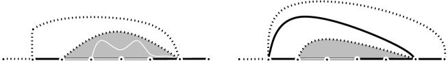
In this paragraph . We reveal the triangle that contains the root edge in . Two cases may occur:
-
•
The revealed triangle could simply be a triangle with a third vertex lying in the interior of , see Figure 3(a). This event appears with probability which we denote by , and it is easy to see from the convergences (1) and (2) the asymptotics (4) and (5) that
We deduce that and .
Furthermore, conditionally on this event, the remaining triangulation (in light gray in Figure 3) has the same distribution as . To be precise, we need to specify a root for this new map, but due to the translation invariance discussed above, any boundary edge will do. For example we may root it at the edge of the revealed triangle which is adjacent on the left of the original root edge.
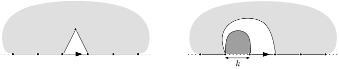
Figure 3: Cases when peeling a triangulation. The map in the light gray area has the same law as the entire map. -
•
Otherwise, the revealed triangle has all of its three vertices lying on the boundary and the third one is either edges to the left of the root edge or edges to the right of the root edge, see Figure 3(b). These two events have the same probability which we denote by . Notice first that when we must have since loops are not allowed. Here also, one can use (1) and (2) to compute , and we get
Furthermore, conditionally on the fact that the revealed triangle has its third vertex lying edges away from the root edge, the triangulation with finite simple boundary it encloses (in dark gray on Figure 3(b)) is distributed according to a -Boltzmann of the -gon. The remaining infinite part (in light gray on the figure) with arbitrary choice of root, is independent of the finite map enclosed and is distributed according to . The edges separating the root edge from the third vertex are called the swallowed boundary.
Quadrangulation case.
Let be a half-plane UIPQ and let us reveal the quadrangle that contains the root edge. We have three different cases.
-
•
The simplest of all is the case when the quadrangle containing the root edge has two of its vertices lying inside . As for triangulations, we may compute the probability of this event to be
Here also, conditionally on this event, the remaining half-plane quadrangulation (rooted arbitrarily at the first edge of the revealed quadrangle) is distributed according to .
![[Uncaptioned image]](/html/1301.5311/assets/x4.png)
-
•
The revealed square could also have three vertices lying on the boundary of the map and one in the interior and separate the map into a region with a finite boundary and one with an infinite boundary. This again separates into two sub-cases depending whether the third vertex is lying on the left or on the right of the root edge, by symmetry these events have the same probability. Suppose for example that the vertex is on the left of the root edge. This further splits according to whether the fourth vertex of the quadrangle lies on the boundary of the finite region or of the infinite region. Since all quadrangulations are bipartite, this is determined by the parity of the number of edges between this third point on the boundary and the root edge, which we denote by when odd and by when even (see figure below).
![[Uncaptioned image]](/html/1301.5311/assets/x5.png)
If – the length of the swallowed boundary – is odd then the fourth point of the discovered square lies on the boundary which is exposed to infinity. This event has a probability
On the other hand, if – the length of the swallowed boundary – is even then the fourth point of the square must lie in the enclosed region and this event has a probability
In both cases, conditionally on any of these events the enclosed maps are -Boltzmann of the -gon where or and the infinite remaining part is independent of it and has the same distribution as .
-
•
The last case to consider is when the revealed square has all of its four vertices on the boundary. This could happen in three ways, as , , or vertices could be to the right of the root edge (see Figure 4). In this case the revealed quadrangle separates from infinity two segments along the boundary of lengths and as depicted on the figure below. The numbers and must both be odd. These events have the same probability
As in all other cases, conditionally on any of these events the three components are independent, the finite ones are -Boltzmann of proper perimeters and the infinite one is distributed as .
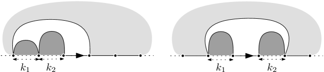
Figure 4: Two of the ways a revealed quadrangle may have all its vertices on the boundary.
General case.
This method applies to more general maps, including -angulations for any (odd or even) as well as maps with mixed face sizes and a weight for each face size. In complete generality the analogues of (4) and (5) are not known, though they are believed to hold, and are known in some cases, most notably fairly general bipartite maps [12]. In any class of maps where these asymptotics hold, a similar peeling procedure may be applied. The number of cases grows exponentially in , as each vertex of the revealed face may or may not be on the boundary, and in general some of the vertices may coincide. However, the separated components of the map are always independent Boltzmann maps, and are independent of the remaining infinite part which is distributed as the half-plane model. While the computational complexity of such analysis increases quickly with , it seems there is no conceptual difficulty involved in generalizing our arguments to any specific .
2.3.2 Starring
Although the one-step peeling transitions in the cases of triangulations and quadrangulations seem different they share several common key properties which specify here. To this end, let us introduce a few notions. Imagine that we reveal the face adjacent to the root edge in as above. The new face may enclose a finite region (or two) and can surround some of the edges of . We call these edges the swallowed edges.
On the other hand, some edges of the new discovered face form a part of the boundary of the remaining half-planar map. These edges are called exposed edges. In the triangulation case there are two exposed edges when the discovered triangle has only two vertices lying on the boundary (first case) and one exposed edge otherwise. In the quadrangulation there are three exposed edges on the event of probability , two exposed edges on the events of probabilities for odd and only one on the events of probabilities for even and . See Figure 5.

Let respectively be the number of exposed edges and the number of edges swallowed to the right of the peeling point when revealing a single face. By symmetry, the number of edges swallowed to the left of the peeling location has the same distribution as . Of course, the number of edges swallowed on the two sides, and are not independent. We now define
| (6) |
We will see that plays a key role in determining percolation thresholds on these infinite maps.
Proposition 3.
We have
| and | (7) |
Moreover, for we have
| (8) |
Proof.
Both statements follow from a direct computation using the exact expression of the probabilities and the enumerative formulae of the last section. We omit the details, though the result is easily and reliably verified in a computer algebra system such as Mathematica™ or Maple™. ∎
Remark.
The identity (7) should hold for any reasonable class of planar maps. It would be nice to have a conceptual explanation for it, rather than a computational proof, perhaps in terms of singularities of generating functions.
Note that in the triangulation case this implies that is simply equal to , since . The relation between the expected number of swallowed and exposed edges can also be interpreted as follows. During the exploration of a face the change in the length of the boundary of the external infinite half-plane map has zero expectation. Indeed the initial edge at which we peel, together with the swallowed edges are no longer on the boundary, and the exposed edges are added.
Note however that the number of exposed edges is always bounded by in the triangulation case and by in the quadrangulation case, whereas the number of swallowed edges has a heavy tail. Indeed, has a heavy-tail of index that is
In particular, is in the domain of attraction of a spectrally negative -stable random variable, a fact we use in Section 4.
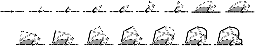
2.3.3 Markovian exploration: the peeling process
Based on the description of the one-step peeling of the root edge one can define a growth algorithm for random maps, the peeling process, that was first used heuristically by physicists (see [32] and [3, Section 4.7]) in the theory of dynamical triangulations. Angel [4, 5] then defined it rigorously and used it to study the volume growth and site percolation on the uniform infinite planar triangulation for . See also [9] where the peeling has been used to study the simple random walk on the UIPQ. We adapt these ideas to the context of half-plane UIP.
Let be an infinite -angulation with an infinite simple boundary. If is an edge on the boundary of we denote the one-step peeling outcome by . This is the map obtained from by “removing” the submap made of the face adjacent to together with any finite regions this face encloses, see Section 2.3.1. This map is rooted as in the previous section.
A peeling process is a randomized algorithm that consists of exploring by revealing at each step one face, together with any finite regions that it encloses. More precisely, it can be defined as a sequence of infinite -angulations with infinite boundary such that for all
for a (necessarily unique) edge on the boundary of . We denote the revealed part by . This consists of all faces of not in , and all vertices and edges contained in them. Moreover the choice of the edge should be independent of the unrevealed part . That is can be chosen by looking at the revealed part made of the union of all the faces revealed and the finite regions they enclose up to step and possibly an independent source of randomness which is independent of . Note that many different algorithms can be used in order to choose the next edge to reveal. The only constraint is that we do not used information from the undiscovered part. Under these hypotheses we have
Proposition 4.
Let be a peeling process then
-
1.
for every , is distributed as and is independent of ,
-
2.
the sequence of pairs representing the number of exposed edges and the number of edges swallowed to the right of the peeling edge for is an i.i.d. sequence with mean given by Proposition 3,
-
3.
for these have distribution
The explicit distribution of can be computed from the description and formulae in Section 2.3.1, but will not be used in the following.
Proof.
We prove the first statement by induction. Suppose that at step the as yet unrevealed part is independent of the revealed part and is distributed as a standard UIHP. We then pick an edge on the boundary of . Since the choice of this edge is independent of itself, the map obtained by re-rooting at is also distributed as the UIHP. We can thus reveal the face in adjacent to this edge and deduce from the previous section that is independent of the union of and of the finite regions discovered by this operation.
The second point easily follows from these considerations, and the third from the description of above. The additional term in the case comes from the event that the revealed triangle has its third vertex to the left of the root edge, which has probability . ∎
3 Percolation thresholds
We now use the peeling exploration described in the last section in order to study percolation on UIHP. The key idea being as in [5] to explore the (leftmost) percolation interface. But this needs some care and tricks depending on the type of percolation and lattice considered.
To help the reader getting used to the tools and methods, we start by recalling the exploration of percolation interfaces in site percolation on triangulations as developed in [4, 5]. We then generalize this exploration process to treat the case of face and bond percolations on UIHP. As we will see, the exploration of site-percolation interfaces is possible in the triangular lattice, but present methods fail for more general lattices. On the other hand our exploration of face and bond percolations can be performed in virtually any class of map.
We begin with Theorems 5, 6, 7 and 8, where we study the cluster of the origin with special boundary conditions. The structure of the proof of each of these theorems is as follows: First we introduce a special boundary condition and a peeling algorithm. We then check that the process leaves the form of the boundary condition invariant and check that the exploration is Markovian in the sense of the previous section. For each model, a planar topological argument shows that the peeling stops if and only if the cluster of the origin is finite. We finally relate the length of the “active boundary” during this exploration to a random walk whose increments have a computable mean expressed in terms of and only. The peeling threshold is given when these increments have zero mean. Proposition 9 then proves that the threshold probabilities found in these results indeed correspond to the quenched critical probabilities for percolation in the standard models.
3.1 Site percolation on triangulations
Let for be a UIHPT. Suppose that conditionally on we color the vertices of with two colors (black and white) as follows: We first color deterministically all the vertices of the boundary in black except the extremity of the root edge that we color in white. We then color all the remaining vertices independently in white with probability and in black with probability . This yields site percolation on with mostly black boundary condition, except for a single vertex. Our goal is to study the white cluster containing the only white vertex of the boundary. We shall use when there is no risk of confusion, and make explicit the type of lattice and percolation only when needed.
Proof.
The central idea is to explore along the (leftmost) percolation interface using a peeling procedure. Let us describe precisely the algorithm to choose the edges to peel:
Algorithm: Assume that is a site-percolated UIHP with a boundary condition of the form (i.e. all white vertices form a single finite connected segment). Peel the edge (which is well defined on the assumption). If the peeling of discovers a new vertex inside (case in Section 2.3.1) then also reveal the color of this new vertex.
There are a couple of easy facts to check to see that this indeed defines a peeling process. First, it is easy to see that the form of the boundary condition black–white–black is preserved after peeling at the edge and possibly revealing the color of a new vertex. Here we use the fact that is a triangulation. Second, the edge chosen to be peeled at time indeed depends on the submap discovered up to time as well as on the color of its vertices but clearly does not depend on , nor on the color of its internal vertices. Hence Proposition 4 applies, at least as long as the boundary of contains a white region necessary to designate the next point to peel.
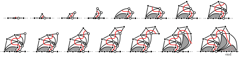
It is easy to check that if this peeling algorithm is used from the very beginning then all the white vertices on the boundary of are part of the cluster of the white origin vertex. This exploration process terminates at the first peeling step when the white boundary is “swallowed”, that is, when the new discovered triangle makes a jump to the right of the peeling point and reaches the black boundary. If that happens, a simple topological argument shows that the white cluster must be finite (see Figure 6). If the process does not terminate then is infinite.
Let for be the number of white vertices on the boundary of . Thus . If then is defined and positive for all . On the other hand, if is finite then for some , after which the above peeling process is no longer defined. (For completeness, we let for all in that case.)
We let if the peeling of discovers a new vertex inside and if the color of this vertex is white, set otherwise. Notice that conditionally on the fact that the face adjacent to in has a vertex lying inside (that is we discover two exposed edges) then is a Bernoulli variable of parameter , and is independent of and of its coloring.
Recall that are the number of exposed and swallowed edges during the th step of peeling, and that as long as the white interface is not empty these are i.i.d. random variables whose distribution is given in Proposition 4. Then we have the following relation between the sequences defined so far that holds for :
| (9) |
as long as (where ), see Figure 7.
Hence the process is a random walk with i.i.d. steps starting from and killed (and set to ) at the first hitting time of . Furthermore the increments of this walk have mean
It follows that the cluster is almost surely finite if and only if , thus for and that the cluster of the origin is finite at . ∎
Interface. It is easy to see that the above peeling process just explores the leftmost interface of the cluster of the origin. More precisely, there is a well defined path in the dual graph separating from the black cluster containing the left part of the boundary. At each step of the peeling process we reveal a face along this interface. We also discover the color of the vertices in the same time we peel . Faces visited by the interface correspond to peeling steps except that part of the interface that is contained in the triangulation enclosed by the last jump (in dotted red line on Figure 6).
Remark.
Note that it is essential that is a triangulation for the exploration of the interface of site percolation to work. Indeed the boundary condition black–white–black may not be conserved during an exploration of site percolation on quadrangulations or other maps. We do not know how to adapt these ideas for quadrangulations, and the value of is unknown. Note also that the fact that for triangulations is not surprising since site percolation is self-dual on any triangulation.
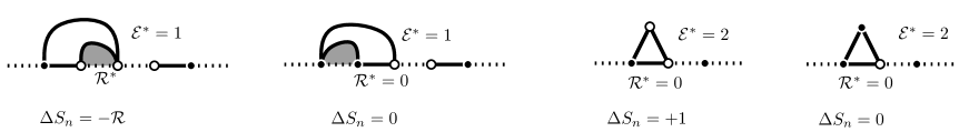
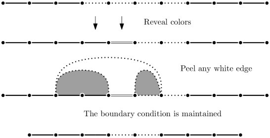
3.2 Face percolation
We now use similar arguments to study face percolation on UIHP (two faces are adjacent if they share an edge). Equivalently this is site percolation on their dual lattices. This time we are not restricted to the triangulation case. Our results are valid for , and there is no serious obstacle to deriving them for more general maps.
Let each face of be colored independently white with probability and black otherwise. Face percolation does not have any apparent boundary condition, but in a sense we explain now, it does. Let us color the infinite external face in black, which corresponds to an all black boundary condition. As far as percolation clusters are concerned, this is equivalent to adding an extra face adjacent to each boundary edge and colouring it black. We do this for all boundary edges except for the root edge. For the root edge, we add a white external face see Figure 8. We now consider to be the white cluster of this “origin face”, and show that it is a.s. finite if and only if .
Theorem 6.
We have if and only if where
Proof.
We adapt the exploration process of the last section. Having added the starting white face outside and after coloring the infinite remaining face in black we have a black–white–black boundary condition similar to the situation with site-percolation. Each edge of is incident to one face inside and one outside of . The form of the boundary conditions that we maintain is as follows:
Algorithm: Assume that the boundary of is of the following form: there is a single connected finite segment along the boundary adjacent to white external faces and all other edges are adjacent to black faces. That is we have a black–white–black boundary condition. We then peel the leftmost edge of the white part and reveal the color of the discovered face.
Here also a few checkings are in order. The initial boundary condition is trivially of the required form. Second, notice that the boundary condition black–white–black is preserved by the peeling of the leftmost “white” edge, and this is valid for (and indeed for any planar map). Next, as before, the choice of the edge to peel stays independent of the unknown region and of its coloring.
If this algorithm is used from the beginning then every edge on the boundary of that is adjacent to a white face of is actually connected is the dual of the map to the origin white face. Here also the exploration stops when there is no edge to peel and a simple topological argument shows that this happens after a finite number of steps precisely when the white cluster of the origin is surrounded by black faces and is consequently finite. Otherwise the peeling process goes on forever (see Figure 8).
During this exploration process, we still denote by respectively the number of exposed edges and the number of edges swallowed on the right of in the th peeling step. We also let if the face discovered at time is white and otherwise. Hence, the process is just a sequence of i.i.d. Bernoulli variables with parameter , and are independent of .
Let denote the number of edges on the boundary of (or equivalently ) adjacent to a white face, and let be absorbed at . Then we have and as long as
| (10) |
Thus the process is almost but not quite a random walk with i.i.d. increments killed at the first hitting time of . In particular, as long as is above for triangulations or for quadrangulations, its previous increment is just . Still, it is easy to see that will a.s. reach if and only if
which completes the proof. ∎
Interface. In this case also, the above peeling process roughly follows the leftmost interface of the origin cluster. However, contrary to site percolation on triangulation some parts of the interface (even before the last jump) are not explored and are contained in enclosed maps: see the red dotted line in dark gray parts on Figure 8.
3.3 Bond percolation
We now turn to bond percolation. Let us present the setting which is very similar to the ones treated before. Let . To treat bond percolation a new type of boundary condition will be required. Conditionally on we color the edges of with two colors (black and white) with special boundary conditions: The root edge, and every edge to its right along the boundary are black. Every other edge of the map is colored white with probability and black with probability independently. Thus the boundary is half-free and half-black. We are interested in : the connected white cluster of the root vertex (the tail of the root edge).
Theorem 7.
We have if and only if where
Proof.
When dealing with bond percolation a new important idea is to keep as much randomness as we can. Thus we do not reveal the status (white or black) of all the edges we discover and keep most of them as unknown. Instead we only check the color of an edge when necessary to determine if this edge is part of or not. More precisely, we again maintain a certain boundary condition on .
One further difference is that we do not reveal a face of the map at every step. Instead, on some steps we only reveal the color of an edge. Thus for some we will have that , except for differing boundary conditions.
Algorithm: Assume is a bond-percolated UIHP with a boundary condition of the following form: There is a single finite segment of boundary edges that are white (possibly of length ). All edges to the right of this segment are black, and all edges to their left are unknown and are i.i.d. with probability of being white (and also independent of the remaining map and its inside coloring). That is we have a free-white-black boundary condition. We then reveal the color of the rightmost unknown edge . If (and only if) it is black, we also perform a peeling step at that edge and reveal a face of without revealing the status of the new edges discovered.
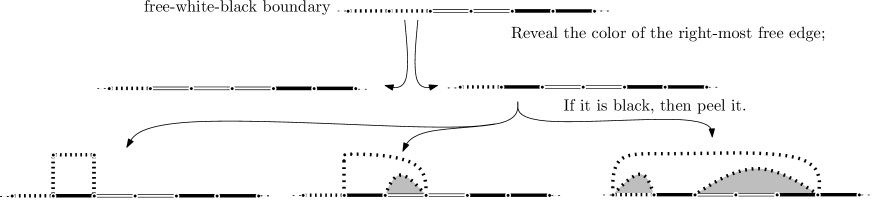
It is again straightforward to check that this form of boundary conditions free-white-black is preserved under the peeling process (this holds for any class of map) and that the starting boundary condition is of the required type (a single origin vertex with white edges), see Figure 9. We will further assume that this algorithm is used from the beginning.
Contrary to the previous cases, there is no clear stopping time for the process because there is always a rightmost unknown edge to reveal. In fact even if at some peeling time the whole white boundary is eaten there is still a possibility that the new vertex at the junction free-black is linked to the white cluster, see Figure 10. However as soon as it is easy to see that if at time the white boundary is of length then there is a strictly positive probability that at time the rightmost unknown edge turns out to be black and the revealed face blocks the white cluster that is, even the new junction free-black vertex is not part of the white origin cluster. See Figure 10. In this case the white cluster of the origin is finite.
Let be the number of edges in the white boundary segment of , so that initially . Let be the indicator of the event that the edge tested in step is white, and let be the number of edges swallowed to the right of . Note that if is white then no face is revealed and by convention we let in this case. We do not need in this model. Then we find that satisfies
and is defined for all . According to the previous considerations if infinitely often then almost surely. On the other hand if for all but finitely many , then there is a positive probability that a.s. The expected increment of is which is positive precisely when . The theorem follows. ∎
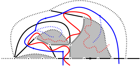
Interface. It is useful to consider simultaneously the percolation configuration on the lattice and the dual percolation configuration on the dual lattice. Since each edge of the lattice corresponds to a dual edge in the dual lattice, the randomness is the same. We will use the same colors for an edge and a dual edge, so we study white primary clusters and black dual clusters. The above exploration process just follows the (leftmost) interface of the cluster , that is the interface that separates the cluster of the root vertex from the dual black cluster of the face containing the edge to its left. As in Section 3.2 not every face visited by the interface corresponds to a step of the peeling process and some parts of the interface lie in enclosed maps. See Figure 11.
3.4 Dual percolations
In this section we study the “dual” of the percolations studied in the last sections. By dual percolations we mean that if the origin cluster is blocked this is because there is a “dual” cluster in the dual percolation preventing it from going further. In particular we shall prove the unsurprising result that the corresponding thresholds equal minus the initial ones.
Since site percolation on triangulations is self-dual this case is already solved. As we already noticed, the dual percolation of bond percolation on the UIHP is bond percolation on the dual of the lattice. This process is studied in Section 3.4.1. In Section 3.4.2 we sketch the analysis of the dual of face percolation which is given by site percolation on the “star” lattice associated to .
3.4.1 Dual bond = bond dual
Here we establish the unsurprising result . While the arguments is very similar to the one used in the previous section, we describe it here as an illustration of how going from the primal to the dual lattice and following the same interfaces yields slightly different exploration procedure.
For sake of clarity we stay with the primal lattice but explore the dual cluster of the origin. We will first get the result with a slightly different boundary condition: All the edges of the boundary of the primal but the root edge are black. The root edge and all edges not on the boundary of are independent and randomly colored, white with probability and black with probability . Recall that the color of a dual edge is that of its corresponding primal edge. We are now interested in the dual white bond percolation cluster containing the dual of the root edge, which by convention is empty if the root edge is black.
Theorem 8.
We have if and only if where
Proof.
As for bond percolation, the color of some edges will remain unknown. At each step we shall reveal the color of one edge whose status is still unknown, and possibly reveal additionally a face of the map. The preserved boundary condition is now black-free-black.
Algorithm: Assume is a bond-percolated UIHP with a boundary condition of the following form: All the edges are black except a finite connected white region of finitely many edges whose unknown colors are i.i.d. white with probability and black with probability (and also independent of the unknown region). We then discover the color of the leftmost edge with unknown color. If it is black we do nothing more. If it is white, we also discover the face in adjacent to it but do not reveal the status of the new edges.
Clearly is of the above form and as usual we see that the boundary condition black-free-black is preserved under the peeling process (see Figure 12), at least as long as unknown edges are present on the boundary. Again, this is valid without any restriction on the type of maps considered.
If the process is used from the beginning up to time , then one can check that every edge of unknown color on that turns out to be white is connected in the dual of to the dual root edge (if it is white). The process stops when there are no more unknown edges at some stage and as usual, a planar topological argument shows that this happens precisely when the dual white cluster of the origin edge is finite.
Let us denote by the number of edges of unknown color on the boundary after steps of the peeling process. Let be the indicator of the event that the edge inspected at step is white, and let denote the swallowed and exposed edges as before, with the convention that both are if no face is revealed in the th step. Clearly and as long as we have
As before is killed and set to when reaching . Hence is not exactly a random walk absorbed at but the increments are independent as long as is large. In particular we see that has a positive probability of remaining positive if and only if
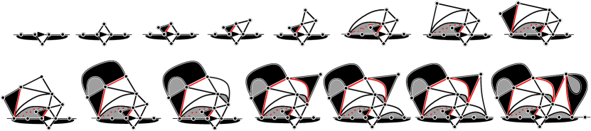
3.4.2 Dual face
Face percolation is not self-dual. If two faces have only a common vertex but no common edge, they need not be part of a single connected white cluster, but if two such faces are black they do form a local barrier for connection of white faces. Hence the dual percolation of face percolation is face percolation but where two faces are declared adjacent if they share a vertex. Equivalently it corresponds to site percolation on the dual lattice where we add connections between sites whose dual faces share a vertex. This is known as the star-lattice in the case of . We call it face′ percolation in the sequel.
We have the expected result
Since the reader has already seen several versions of this argument, we only sketch the proof: The preserved boundary condition is now black–white–black (that is edges are adjacent to exterior faces of those colors). The white part may be empty, in which case we consider it to include a single vertex. The peeling rule is to peel at the edge just to the left of the white revealed part. The corresponding recursion for the length of the white boundary is
As in Section 3.3 even if the white part is swallowed in the process, it could be that the vertex at the junction enables the origin cluster to grow further. The problem is treated similarly and as long as we have infinitely often and then a.s. Otherwise with positive probability. We leave the details to the interested reader.
3.5 Free boundary conditions, universality
In Theorems 5, 6, 7 and 8 we focused on the cluster of a single boundary point (or edge or face) with specially chosen boundary conditions: black for site percolation on triangular lattice, black for face, face′ and dual bond percolation and free–black for bond percolation. Note that black boundary condition is the natural setting for studying the white cluster of the origin in face percolation because of the presence of the infinite root face which cannot be part of (otherwise, is trivially infinite). The same remark holds for dual bond and face′ percolation. However, one can wonder whether free boundary condition (that is all edges or vertices have i.i.d. colors) changes the percolation threshold in Theorems 5 and 7. The answer is no:
Proposition 9.
The percolation thresholds and identified in Theorems 5 and 7 correspond to the a.s. thresholds for percolation on the corresponding percolations on the half-planar maps with free boundary conditions.
Proof.
Let us focus on the case of bond percolation with free boundary condition. Imagine that we reveal the right neighbors of the root edge until we find a black edge. At this point we have a free–white–black–free boundary. We then run our exploration process at the free–white junction. If then there will be some time where the white boundary is completely swallowed. At this stage, as in the proof of Theorem 7, there is a positive probability that the next stage of the exploration totally blocks the cluster of the origin which is thus finite. If it is not the case we just continue the exploration process at the junction. We eventually end-up with a blocking situation. Clearly if for every vertex of the boundary the probability that is in an infinite white cluster is then there is no percolation on the full-map. If there is a positive probability that the cluster of the origin is infinite. By ergodicity of the half planar maps w.r.t. the translation operator (that preserves the map but shifts the root edge along the boundary) we deduce that in this case there is percolation on the map.
The case of site percolation involves similar ideas, although proving that there is no percolation at critically is a bit more tedious. We safely leave the details to the interested reader. ∎
Universality.
Whereas the exploration of site percolation of Theorem 5 is specific to the triangulation case, we have already indicated in the proofs and at the beginning of Section 3 that the methods developed for bond and face percolations can be applied to any kind of planar maps without restriction on the shape of a face.
In [6] we will prove that the percolation thresholds identified in this work also correspond to percolation thresholds for the corresponding models on the full-plane UIP.
4 Critical and off-critical percolation exponents
We now show how peeling along percolation interfaces allows us to deduce certain geometrical properties of the percolation clusters and in particular compute certain critical exponents. For sake of simplicity we focus on the simplest case which is site percolation on the triangular lattice . Thus we fix , and omit it from notation. We shall comment in Section 4.3 on the adaptations needed for our proofs to cover more general cases.
Recall the setting of Section 3.1: Let be a half-plane UIPT endowed with Bernoulli site percolation of parameter (for white) with boundary condition given by the infinite boundary being black with the exception of the root vertex which is white. Theorem 5 states that the probability that the cluster containing the only white vertex of the boundary is infinite is positive if and only if . More precisely, we have from (9) that the length of the white boundary during the exploration process evolves as a random walk with i.i.d. increments of law
where the joint law of is given by Proposition 3 and is an independent Bernoulli variable of parameter . The process starts at and is killed at the first entrance of . In particular takes its values in and satisfies for
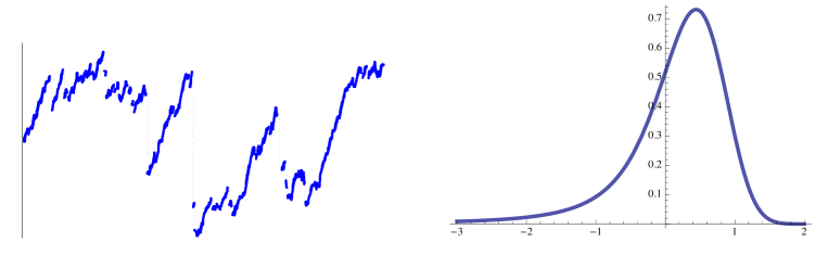
When the increments have mean . In this case we simply write for . Since the r.v. is in the domain of attraction of a stable random variable, the associated (unkilled) random walk converges once renormalized towards a stable process of parameter . Let us be a bit more precise and recall some background about the spectrally negative -stable process and its discrete version. The interested reader should consult [11] and the references therein for more details.
We slightly abuse notation here and consider the walk not killed at the first entrance of that is, let and be a random walk with i.i.d. increments of law then we have
where is the standard -stable process with no drift and no positive jumps with and the convergence holds in distribution for the Skorokhod topology.
By standard spectrally negative -stable process, we mean that its Laplace transform is given by for all , equivalently its Levy measure is given by
This process is also known as the Airy-stable process and as the (map-)Airy distribution. Note that the Airy distribution is not symmetric, has stretched exponential tail on the right but power law tail on the left, see Figure 14. This process enjoys the scaling property with parameter that is in distribution for any . By the scaling property, the positivity probability is independent of and equals
This quantity is of great importance since it rules the behavior of many distributional properties of and its discrete analog .
4.1 The off-critical percolation probability
A first application is the exact computation in of the probability that the cluster is infinite.
Theorem 10.
For site percolation on with black boundary conditions except for a white root vertex, we have
In particular this implies that the off-critical exponent for the percolation probability is (which means for ). Note that if the root vertex is instead taken to be random, the percolation probability becomes simply .
It is perhaps surprising that the probability of percolation tends to as . This comes from the fact that even if (that is, every new discovered point is white) there is still a non-zero probability that the first step (or first few steps) of peeling swallows the white boundary by making a connection towards the right and swallowing the white cluster.
Proof.
By (9) in the proof of Theorem 5, the probability that the cluster of the single white point on the boundary of is infinite is equal to the probability that a random walk starting from and with i.i.d. increments distributed as never hits . In our very specific case this probability can be evaluated exactly. Indeed, if are i.i.d. copies of we have
We have that . Since , the ballot theorem (see e.g. [1, Theorem 3]) implies that is equal to the mean of which is . This finishes the proof of the theorem. ∎
4.2 Critical exponents
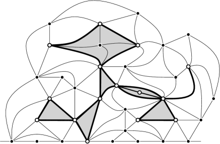
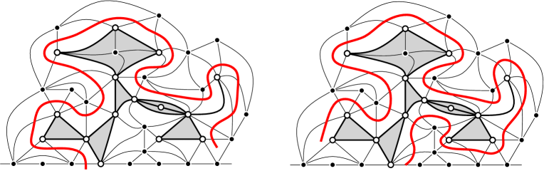
We now turn to the study of the geometry of the cluster for site percolation on at the critical point . Recall that the cluster of the only white vertex of the boundary is almost surely finite at . We denote by the hull of that is the sub map of obtained by filling-in all the finite holes of . This hull has a connected boundary made of white vertices which we denote by (unlike the boundary of which may have any number of connected components). We also consider the extended hull of the cluster which is made of the hull of all triangles adjacent to (see Figure 2) or equivalently of the hull of the triangles discovered during the exploration process (see Figure 15 below). This has the effect of adding to any so-called fjords, or parts of the complement connected to infinity only through a single vertex.
We are interested in the boundary of w.r.t. , that is the number of vertices in adjacent to a vertex outside . Note that part of the perimeter of coincides with the boundary of . That part of the perimeter is not included in our estimates. Considering the full boundary of would not change the critical exponents but would require some additional arguments. In fact, this part of the perimeter has the same scale as the rest of the perimeter.
Before going into the proof of Theorem 2 let us recall a few facts on random walks in the domain of attraction of a spectrally negative -stable Lévy process. Remember that the length of the white boundary of in the exploration of the cluster of the origin evolves as a random walk started from and with independent increments where the Bernoulli variables have parameter . In particular the negative jumps correspond to . Recall also that is supported on . The hitting time of for such walks has been analyzed by [31] and (combined with [18, Theorem 1 (2.4)]) we get
Lemma 11 (Hitting time of ).
If is the hitting time of by , then we have
for some (with an explicit but not useful formula).
We shall also need an estimate on the fluctuations of sums of i.i.d. variables of this type. This is a standard type of result, but we were not able to locate a precise reference, so we include a quick proof.
Lemma 12 (Exponential tail on the right).
There exists such that for every and for every we have for as above
In fact, it should be possible to improve the bound to , which would lead to improved powers of in some of the bounds we get for Theorem 2.
Proof.
Using the tail asymptotic of we have for
for some . Applying an exponential Markov inequality after multiplying by we get
Proof of Theorem 2.
We have sorted – according to the value of the critical exponent but we prove first then and finally . In order to lighten notation and spare use the introduction of constants we use the symbol if there exists some universal constant such that for all
: The hull’s perimeter.
The peeling exploration of the cluster of the origin follows the contour of the cluster keeping it on the right. In particular, the number of steps of peeling necessary to explore the cluster of the origin is thus the number of triangles adjacent to , which is easily related to the size of below. There is a slight problem arising at the last step of the exploration. The exploration reveals enough of the map to guarantee that the cluster is finite, but does not enter the region surrounded by the last jump, see Figure 15 below.
This problem can be circumvented by using a rightmost exploration process as depicted in the figure. This is just a mirror image of the process, and since the is symmetric in distribution, this dual exploration has the same law as the original one. Thus if we denote by (resp. ) the number of steps of peeling when discovering the cluster clockwise (resp. counterclockwise) and if denotes the number of triangles on the boundary of then we have
By the description of the peeling process in the triangulation case, both and are distributed according as (though they are not independent!). Since each triangle is incident to at most vertices of , Lemma 11 now implies that .
For the lower bound, observe that at each step of the peeling the probability of having is some constant ( as it happens). Thus the number of triangles on the interface incident to any vertex of is dominated by a geometric random variable. Moreover, these dominating random variables may be made independent. (That is, there is a coupling of independent geometric variables and the map so that the domination holds a.s.) By a standard large deviation estimate for sums of random variables, for suitable constants,
With Lemma 11 this gives the lower bound.
: The hull’s volume.
The volume of the hull , can be measured in vertices or faces. We work below with vertices, though the two are directly connected for triangulations in terms of the boundary which is smaller by , and so the number of faces is of the same order of magnitude. Faces have a slight advantage of in that faces are added to the hull in one way only, as the enclosed triangulations encountered on the right of the peeling process when we enclose a region and fill it in with a Boltzmann triangulation of the proper perimeter, whereas vertices may also be on the boundary. Special care is needed again for the last peeling step because the triangulation put inside the last peeling step is not entirely contained in the hull.
Let be the number of vertices added to the hull in the th step. This is when a new internal vertex is discovered. When , this is the number of internal vertices in the Boltzmann map added, except at the last step when only part of that map is in the hull. Thus we have
A simple observation using the formulae for shows that a Boltzmann triangulation with perimeter typically has a size of order . More precisely from [5, Proposition 5.1] and [5, Proposition 6.4] there exists such that for all and we have
| (11) |
for some . In fact by [5, Proposition 6.4] the distribution of the size of a Boltzmann triangulation of perimeter renormalized by converges towards a Lévy distribution.
For the lower bound, we exhibit a way for to have size with probability of order : First the peeling process continues for at least steps that is . This has probability of order by Lemma 11. On this event, there are typically (several) times before when is of order , so with probability bounded from there is at least one such jump of size at least . Such a jump adds to the hull a Boltzmann triangulation of perimeter of order which is typically of size by (11). Thus on the event that there is at least a constant probability that , and so for some .
Informally, the reason this is the typical way of getting a large hull is that it is easier to make even larger (exponent ) than to have smaller and have an unusually large Boltzmann map (exponent ). It is also possible to have small and no abnormally large Boltzmann map, but this requires the discrete stable process to behave badly, which is even less likely.
To prove the corresponding upper bound we start by ignoring the last step , and first split according to :
The first summand is at most a constant times , so we focus on the second and apply Markov’s inequality:
Using (11) we have that (allowing for ). So after conditioning on and taking the terms outside the sum we end-up with
To compute the we need first to truncate it. On the event we have (since increases by at most at each step). By Lemma 12 we have that . Thus with very high probability (super-polynomially close to )
This allows us to truncate the s: for some we have
The next step is to separate the restriction to . For this we observe that the events and are negatively correlated since a larger negative jump can only help the process hitting . Thus conditioning on stochastically decreases and we have
where we have used the tail distribution of and the easy estimate . Plugging this in we find
This almost completes the proof. It remains to show that the contribution from the last step when hits is also unlikely to be large. Here we do not have because of the undershoot below . Let us call this last jump and let be the size of the Boltzmann map added during this last jump. Again, we may restrict to the event and shall split according to the value of . By (11) we have
On the other hand we have for
Using Lemma 12 and the bound we have so . Finally
: The hull’s perimeter, excluding fjords.
In order to study we consider the evolution of the boundary of as the peeling process progresses. A new difficulty is that only after the process has terminated we can tell with certainty whether any particular vertex is in or not. As we follow the peeling process, newly revealed black vertices are added tentatively to , but are removed from it if they are in a part of the boundary that is swallowed by a connection to the left of the peeling edge.
In order to control the tail of , let us introduce an auxiliary process , which follows the evolution of the black boundary left of . This length is of course infinite always, so instead we follow only the change of this boundary, in the form of vertices added and removed from the boundary. Formally let be the number of edges swallowed on the left of the th peeling point. We have that have the same law as , though is not independent of . Recall also that is the indicator of the event that this new vertex is white. We form the process by putting and
Thus is just a random walk with i.i.d. increments distributed as . Note that the two walks and are not independent, since they use the same and sequences, and since when , are not independent.
With this notation we can determine from and . Whenever reaches its infimum, all the black vertices discovered so far are swallowed. The vertices tentatively in correspond exactly to increments of above its infimum. Thus if we denote , then
While the processes and (and in particular ) are not precisely independent, they are quite close to independent in the following sense. Recall that we are considering only triangulations for now, so either or (possibly both). Since newly discovered vertices are also either black or white but not both, each step of the peeling process changes at most one of and . It follows that if we switch to continuous time with peeling steps controlled by a Poisson clock then the two processes become completely independent. For other tyes of maps and percolation models a slightly weaker form of independence holds (see Section 4.3).
To get a lower bound on , consider the event . This event has probability equal to a constant times by Lemma 11. Conditioned on this event, by the above remarks, the process is roughly distributed as times , where is the Airy-stable process introduced in the beginning of the section, and in particular the conditional probability of is bounded away from .
Let us prove the corresponding upper bound. Since is a sum i.i.d. variables with mean, bounded above by and in the domain of attraction of a -stable variable, we have from Lemma 12 for any that
and so
For the exponential term easily dominates and we have that decays super-polynomially (faster than ). On the other hand, , and the proof is finally complete. ∎
4.3 Universality of critical exponents
In this section we comment on the modifications to make to the previous section if we consider face or bond percolation on general . We endeavor to address all the different difficulties that arise, and some possible ways to overcome them. However, a full proof would involve some nasty details and so we stay at a rather high and (very) imprecise level, and formally state Theorem 2 only for triangulations. May the reader forgive us.
First, the description of the active boundary in the percolation exploration process is no longer exactly a random walk killed uppon hitting . However, it is very closely related to such a process. In particular, as long as is large the increments are i.i.d. It is easy to see that the increments of this walk have mean exactly at the critical point, that the increments are bounded from above and have heavy-tail of exponent on the left (even in the case of quadrangulations where there may be two segments swallowed on the right, as in Figure 4). In particular these increments are always in the domain of attraction of the -stable process with no positive jumps. Obviously, the value of is changed.
Concerning Theorem 10, a similar argument holds for some the other percolation models we discussed, but yields a slightly weaker result. Indeed, for the other models the associated process has increments that are bounded but not by . Thus the ballot theorem does not give the precise probability of eternal positivity. Still, the probability that a random walk on with steps bounded by with expectation remains positive at all times is between and . Thus the identity of the theorem is replaced by lower and upper bounds differing by a constant. In the case of bond percolation, the stopping time of the exploration may not coincide with the first time the active boundary is swallowed but is lower bounded by the preceding and upper bounded by a geometric number of them. All these modifications clearly do not affect the near-critical exponent so that we still have .
Since the tail of the stopping time is also going to be the same, the lower bounds of Theorem 2 are almost unchanged: On the event there is a high probability that , that and .
For the upper bounds, again most of the estimates still hold. Some additional computations arise since it is possible to have multiple Boltzmann maps revealed at a single step, but mostly the arguments hold. Special care is needed for the bound on . Now the processes and are even further from being independent, since it is possible for both of them to make jumps at the same time. However, it is possible to show that the large jumps in these processes occur at distinct times, and so the joint distribution is that of independent processes. This allows one to estimate the fluctuations of above its infimum at the killing time of .
References
- [1] L. Addario-Berry and B. A. Reed, Ballot theorems, old and new, in Horizons of combinatorics, vol. 17 of Bolyai Soc. Math. Stud., Springer, Berlin, 2008, pp. 9–35.
- [2] D. Aldous and J. M. Steele, The objective method: probabilistic combinatorial optimization and local weak convergence, in Probability on discrete structures, vol. 110 of Encyclopaedia Math. Sci., Springer, Berlin, 2004, pp. 1–72.
- [3] J. Ambjørn, B. Durhuus, and T. Jonsson, Quantum geometry, Cambridge Monographs on Mathematical Physics, Cambridge University Press, Cambridge, 1997. A statistical field theory approach.
- [4] O. Angel, Scaling of percolation on infinite planar maps, I, arXiv:0501006.
- [5] , Growth and percolation on the uniform infinite planar triangulation, Geom. Funct. Anal., 13 (2003), pp. 935–974.
- [6] O. Angel and N. Curien, Percolations on infinite random maps II, full-plane models, In preparation.
- [7] O. Angel and G. Ray, Classification of domain Markov half planar maps. 2013.
- [8] O. Angel and O. Schramm, Uniform infinite planar triangulation, Comm. Math. Phys., 241 (2003), pp. 191–213.
- [9] I. Benjamini and N. Curien, Simple random walk on the uniform infinite planar quadrangulation: Subdiffusivity via pioneer points, Geom. Funct. Anal. (to appear).
- [10] I. Benjamini and O. Schramm, Recurrence of distributional limits of finite planar graphs, Electron. J. Probab., 6 (2001), pp. no. 23, 13 pp. (electronic).
- [11] J. Bertoin, Random Fragmentations and Coagulation Processes, no. 102 in Cambridge Studies in Advanced Mathematics, Cambridge University Press, 2006.
- [12] J. Bouttier, P. Di Francesco, and E. Guitter, Planar maps as labeled mobiles, Electron. J. Combin., 11 (2004), pp. Research Paper 69, 27 pp. (electronic).
- [13] J. Bouttier and E. Guitter, Distance statistics in quadrangulations with a boundary, or with a self-avoiding loop, J. Phys. A, 42 (2009), pp. 465208, 44.
- [14] P. Chassaing and B. Durhuus, Local limit of labeled trees and expected volume growth in a random quadrangulation, Ann. Probab., 34 (2006), pp. 879–917.
- [15] N. Curien, J.-F. Le Gall, and G. Miermont, The Brownian plane, arXiv:1204.5921.
- [16] N. Curien, L. Ménard, and G. Miermont, A view from infinity of the uniform infinite planar quadrangulation, Lat. Am. J. Probab. Math. Stat. (to appear).
- [17] N. Curien and G. Miermont, Uniform infinite planar quadrangulations with a boundary, arXiv:1202.5452.
- [18] R. A. Doney, On the exact asymptotic behaviour of the distribution of ladder epochs, Stochastic Process. Appl., 12 (1982), pp. 203–214.
- [19] B. Duplantier and S. Sheffield, Liouville quantum gravity and KPZ, Invent. Math., 185 (2011), pp. 333–393.
- [20] I. P. Goulden and D. M. Jackson, Combinatorial enumeration, A Wiley-Interscience Publication, John Wiley & Sons Inc., New York, 1983. With a foreword by Gian-Carlo Rota, Wiley-Interscience Series in Discrete Mathematics.
- [21] O. Gurel-Gurevich and A. Nachmias, Recurrence of planar graph limits, Ann. Maths (to appear), (2012).
- [22] V. G. Knizhnik, A. M. Polyakov, and A. B. Zamolodchikov, Fractal structure of D-quantum gravity, Modern Phys. Lett. A, 3 (1988), pp. 819–826.
- [23] M. Krikun, Local structure of random quadrangulations, arXiv:0512304.
- [24] , On one property of distances in the infinite random quadrangulation, arXiv:0805.1907.
- [25] , Explicit enumeration of triangulations with multiple boundaries, Electron. J. Combin., 14 (2007), pp. Research Paper 61, 14 pp. (electronic).
- [26] J.-F. Le Gall, Uniqueness and universality of the Brownian map, Ann. Probab. (to appear).
- [27] J.-F. Le Gall and L. Ménard, Scaling limits for the uniform infinite quadrangulation, Illinois J. Math., 54, pp. 1163–1203 (2012).
- [28] J.-F. Marckert and G. Miermont, Invariance principles for random bipartite planar maps, Ann. Probab., 35 (2007), pp. 1642–1705.
- [29] G. Miermont, The Brownian map is the scaling limit of uniform random plane quadrangulations, Acta Math. (to appear).
- [30] G. Schaeffer, Conjugaison d’arbres et cartes combinatoires aléatoires. phd thesis, (1998).
- [31] V. A. Vatutin and V. Wachtel, Local probabilities for random walks conditioned to stay positive, Probab. Theory Related Fields, 143 (2009), pp. 177–217.
- [32] Y. Watabiki, Construction of non-critical string field theory by transfer matrix formalism in dynamical triangulation, Nuclear Phys. B, 441 (1995), pp. 119–163.