Experimental study of libration-driven zonal flows in non-axisymmetric containers
Abstract
Orbital dynamics that lead to longitudinal libration of celestial bodies also result in an elliptically deformed equatorial core-mantle boundary. The non-axisymmetry of the boundary leads to a topographic coupling between the assumed rigid mantle and the underlying low viscosity fluid. The present experimental study investigates the effect of non axisymmetric boundaries on the zonal flow driven by longitudinal libration. For large enough equatorial ellipticity, we report intermittent space-filling turbulence in particular bands of resonant frequency correlated with larger amplitude zonal flow. The mechanism underlying the intermittent turbulence has yet to be unambiguously determined. Nevertheless, recent numerical simulations in triaxial and biaxial ellipsoids suggest that it may be associated with the growth and collapse of an elliptical instability Cébron et al. (2012). Outside of the band of resonance, we find that the background flow is laminar and the zonal flow becomes independent of the geometry at first order, in agreement with a non linear mechanism in the Ekman boundary layer (e.g., Calkins et al., 2010; Sauret and Le Dizès, 2012b).
1 Introduction
Librations, oscillatory motions of the figure axis of a planet, arise through gravitational coupling between a quasi-rigid celestial object and the main gravitational partner about which it orbits Yoder (1995); Comstock and Bills (2003). Several librating bodies also possess a liquid layer, either an iron rich liquid core like on Mercury, Io, Ganymede, and the Earth’s Moon, and/or a subsurface ocean like on Europa, Titan, Callisto, Ganymede and Enceladus Anderson et al. (1996, 1998, 2001); Williams et al. (2001); Spohn and Schubert (2003); Hauck et al. (2004); Breuer et al. (2007); Margot et al. (2007); Williams et al. (2007); Lorenz et al. (2008); Van Hoolst et al. (2008). The interaction of the fluid layer with the surrounding librating solid shell resulting from viscous, topographic, gravitational or electromagnetic coupling leads to dissipation of energy and angular momentum transfer that need to be accounted for in thermal history and orbital dynamics models of these planets.
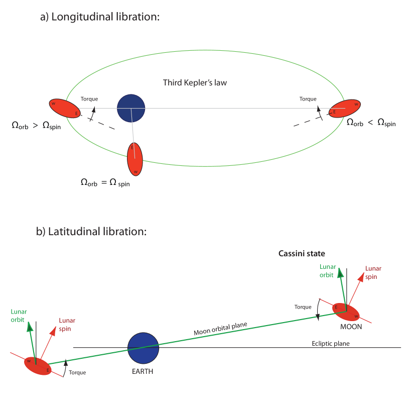
There is a whole variety of celestial objects to which our approach will be applicable, in the next paragraphs we propose to focus on the Earth’s moon purely for pedagogical reasons to clarify some astronomical aspects of the problem and distinguish between the different types of librations. In Figure 1 we illustrate the origin of the gravitational torques producing the librations in the case of the Earth-Moon system considering only the principal harmonic at the orbital period. Over geological time scales, the Lunar mantle has been tidally deformed into a triaxial ellipsoid, resulting in a mass anomaly.
Due to the eccentricity of its orbit, the Moon orbital period varies along the orbit according to the third Kepler’s law. As illustrated on Figure 1a), the induced phase lag between the Earth-Moon direction and the orientation of the equatorial bulge, the so-called optical longitudinal libration, produces a restoring torque along the spin axis of the Lunar mantle. This time periodic torque forces the Moon to physically oscillate axially about its state of mean rotation. This small oscillation is referred to as the physical longitudinal libration. Note that the optical libration is typically of the order of rad whereas the physical libration is only of order rad due to the large inertia of the Lunar mantle.
In addition, the Moon is in a Cassini state, i.e. the relative orientations of the normal to the ecliptic plane, the spin vector of the Moon and the normal to the orbital plane of the Moon are fixed. As illustrated in Figure 1b), it yields a gravitational torque, fixed in the frame rotating with the moon, that tends to align the equator of the Lunar mantle with the orbital plane of the Moon. The spin axis of the Moon being fixed relative to the normal to the orbital plane, the mantle oscillates about an equatorial axis perpendicular to the Earth-Moon direction resulting in the so called physical latitudinal libration. As with longitudinal libration, the physical latitudinal libration is several orders of magnitude smaller than the optical latitudinal libration.
In contrast with precession or nutation that are well represented by gyroscopic motions of the solid shell, it is important to note that librations both in longitude and latitude do not result in changes of the orientation of the spin axis of the planet on diurnal time scales. The combination of optical librations both in longitude and latitude can be observed in an sequence of NASA images of the Moon taken from the Earth along its orbit (http://en.wikipedia.org/wiki/Libration).
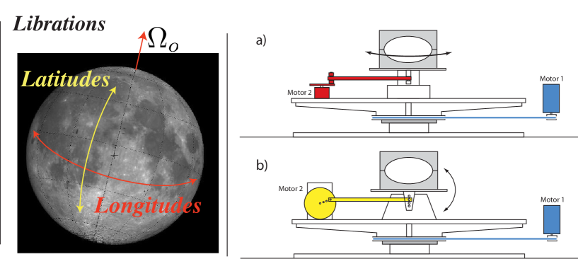
The mechanical forcing produced by the two components of libration that drive the flow in the liquid layer of a planet can be illustrated by two concept laboratory experiments, as illustrated in Figure 2. A turntable mimics the mean rotation of the planet while the oscillation of the planet’s solid shell is achieved by a mechanical system attached to the rotating table. Longitudinal libration, a time periodic oscillation of the body’s figure axis about its mean rotation axis, can be simulated by oscillating the container about the vertical axis (Figure 2a). Latitudinal libration, a time periodic oscillation of the figure axis about an equatorial axis that is fixed in the rotating frame (the turntable), is illustrated in Figure 2b. In the present paper we only consider the flow driven by physical longitudinal libration, herein referred to as longitudinal libration.
Several of experimental, numerical and theoretical studies have been devoted to libration-driven flows in axisymmetric containers to investigate the role of the viscous coupling in librating planets. It has been shown that longitudinal libration in an axisymmetric container can drive inertial modes in the bulk of the fluid as well as boundary layer centrifugal instabilities in the form of Taylor-Görtler rolls Aldridge (1967); Aldridge and Toomre (1969); Aldridge (1975); Tilgner (1999); Noir et al. (2009); Calkins et al. (2010); Noir et al. (2010); Sauret et al. (2012a). In addition, laboratory and numerical studies Aldridge (1967); Wang (1970); Calkins et al. (2010); Noir et al. (2010); Sauret et al. (2010, 2012a) have confirmed that non-linear interactions within the Ekman boundary layers generate a steady, axisymmetric flow, called zonal flow. Analytical derivations of the zonal flow driven by longitudinal libration have been carried out in cylindrical cavity for an arbitrary libration frequency Wang (1970), in spherical geometry at low libration frequency Busse (2010) and more recently in spherical geometry at an arbitrary frequency Sauret and Le Dizès (2012b).
Although practical to isolate the effect of viscous coupling, the spherical approximation of the core-mantle or ice shell-subsurface ocean boundaries, herein generically called the CMB, is not physical from a planetary point of view and very restrictive from a fluid dynamics standpoint. Indeed, due to the rotation of the planet, to the gravitational interactions with companion bodies and to the low order spin-orbit resonance of the librating planets we are considering, the general figure of the CMB must be ellipsoidal with a polar flattening and a tidal bulge pointing on average toward the main gravitational partner (cf. Goldreich and Mitchell, 2010). This assumes that the libration period is far shorter than a typical deformation time scale of the CMB.
In contrast with the spherical or cylindrical geometry, it has been demonstrated analytically that longitudinal libration in a non-axisymmetric spheroid can not produce resonance through direct forcing of a single inertial mode when , where is the ellipticity Zhang et al. (2011). This can be recast as using our notation presented in the next section, which is satisfied for the two non-axisymmetric containers considered in the present study.
Recent analytical and numerical work by Cébron et al. (2012) demonstrates, however, that triadic resonances are possible between two inertial modes and the elliptically deformed basic flow, leading to the so-called Libration Driven Elliptical Instability (LDEI). The elliptical instability can stably saturate in a narrow range of libration amplitude in the immediate vicinity of instability threshold Kerswell and Malkus (1998); Herreman et al. (2009); Cebron et al. (2012). Outside of this limited window, a transition occurs that lead to the development of space-filling turbulence Malkus (1989). This turbulence, which acts to disrupt the elliptically unstable base state, decays and the flow ‘relaminarizes’. The relaminarization phase ends when the base state re-establishes itself. The elliptical instability will then give way again to turbulence. In planetary liquid cores, such an instability could be responsible for an increased viscous dissipation Le Bars et al. (2010), for the induction of a magnetic field Kerswell and Malkus (1998); Herreman et al. (2009), or the presence of a dynamo Le Bars et al. (2011).
Finally, longitudinal libration in a non-axisymmetric ellipsoid can excite instabilities, which develop as the shell rotation is slowing down during the libration cycle Chan et al. (2011), at sufficiently low frequency and large amplitude. In contrast with the side wall centrifugal instability observed in axisymmetric container, the unstable region extends further inside the fluid interior. The underlying mechanism as well as the scaling of the threshold of these instabilities have yet to be investigated via a systematic exploration of the parameter space.
This paper aims at describing the zonal flow driven by longitudinal librations in non-axisymmetric ellipsoidal containers, for which we expect the topographic coupling to be dominant. Spherical and hemispherical containers have been included for comparison to emphasize the effect of the topography.
2 Mathematical background and control parameters
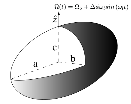
Let us consider a homogeneous, electrically non-conductive and incompressible fluid enclosed in a librating triaxial ellipsoidal cavity. The equation of the ellipsoidal boundary can be written (Figure 3)
| (1) |
where () is a cartesian coordinate system with its origin at the center of the ellipsoid, is along the long equatorial axis , is along the short equatorial axis , and along the rotation axis . We define the ellipticity as
| (2) |
and the aspect ratio
| (3) |
where stands for the mean equatorial radius . In the inertial frame, the longitudinal librating motion of the container can be modeled by a time dependence of its axial rotation rate:
| (4) |
Here, represents the mean rotation rate, is the amplitude of libration in radians and is the angular frequency of libration.
To allow for an easy comparison with previous analytical work, we present the mass conservation and the momentum equations in the frame of reference attached to the librating container. Using as the length scale and as the time scale, these equations are written
| (5) | |||||
| , | (6) | ||||
| (7) |
The first two terms on the left hand side of (5) are the standard material derivative of the velocity field; the third term is the Coriolis acceleration. The right hand terms are, respectively, the pressure force, the viscous force and the Poincaré force. In (5), is the reduced pressure, which includes the time-variable centrifugal acceleration. The Ekman number is defined by
| (8) |
where is the kinematic visosity. The dimensionless libration frequency is defined as
| (9) |
Lastly, is the libration forcing parameter defined by
| (10) |
Typical values of the dimensionless parameters for planets of our solar system are presented in table 2 (courtesy of Noir et al. (2009)). The viscous solution to (5) must satisfy the no-slip boundary condition on the CMB
| (11) |
In the limit of small Ekman number, the flow can be decomposed into an inviscid component in the volume and a boundary layer flow . Introducing this separation, Kerswell and Malkus (1998) proposed the following solution to the inviscid equations of motion subject to the non-penetration condition at the CMB:
| (12) | |||||
| (13) |
The base flow is the sum of a time dependent uniform vorticity flow and a gradient component. It follows that the Reynolds stresses resulting from (12) are balanced by the pressure gradient. Therefore, no net zonal flow can result from the non-linear interactions in the quasi-inviscid interior Busse (2010). However, the no-slip boundary condition (11) is not entirely fulfilled by this inviscid solution. Hence, viscous corrections in the Ekman boundary layer must also be considered. Their non-linear interactions can generate zonal flow in the bulk Wang (1970); Busse (2011, 2010), as already observed in spherical and cylindrical (i.e., axisymmetric) geometries Aldridge (1967); Wang (1970); Calkins et al. (2010); Noir et al. (2010); Sauret et al. (2010, 2012a). In the present paper we use the analytical derivation of the zonal flow from Sauret and Le Dizès (2012b), an outline of the method is presented in the Appendix.
3 Experimental method.
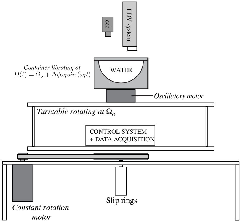
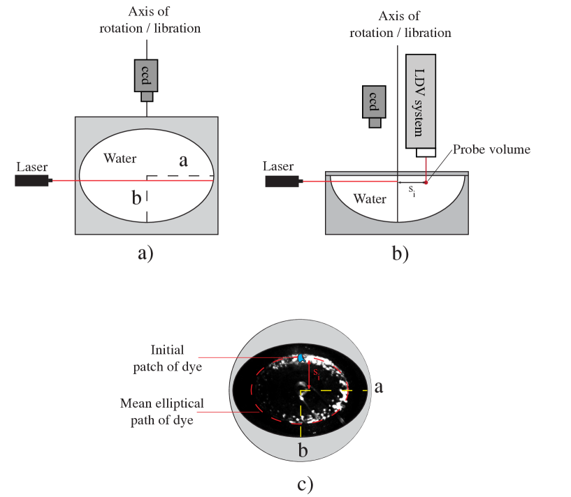
Figure 4 represents a schematic view of the experimental device used in the present study. Except for the containers, the laboratory apparatus is the same as in Noir et al. (2009) (see section 3.1 for a detailed description). The generic set-up consists of a turntable rotating at a constant angular velocity and an oscillating acrylic tank centered on the turntable activated by a brushless direct drive motor. Both rotations are controlled using a motion control system that allows for high accuracy, better than on the mean rotation and on the angular displacement. The container consists of two “hemispheres” CNC machined from cast acrylic cylindrical blocks that are polished optically clear. To characterize the effect of the topographic coupling resulting from the non axisymmetry of the librating body, we use three different containers: i) a sphere of radius mm, ii) a prolate spheroid of long axis mm and short axis mm and iii) a prolate spheroid of long axis mm and short axis mm. These containers correspond to an ellipticity in the equatorial cross section equal to 0, 0.06 and 0.34 respectively. In all three configurations the rotation axis is along c.
We perform direct visualizations of the interior flows using a diluted solution of rheological fluid (Kalliroscope), and a horizontal or vertical laser light sheet. A CCD camera located above the container records movies and still images to characterize the time evolution of the shear structures in the interior. In addition, we use a remotely controlled syringe pump to inject dye (fluorescein or non-diluted Kalliroscope) at a cylindrical radius along the short axis of the mean elliptical equator, i.e. the time averaged figure axis of the equatorial cross-section (see Figure 5c). We then manually track the dye over a full revolution (until it passes by the injection point again) or a fraction of a revolution when the patch spatial coherence is lost due to turbulent mixing. These observations are used to derived the mean angular velocity along the elliptical path followed by the dye as illustrated in Figure 5c. Error bars are obtained by repeating the dye injection several time during the same experiment. Although straightforward, this technique is not suitable when the azimuthal velocity varies on time scale less than a period of revolution of the dye patch.
To address the time dependency of the azimuthal velocity in the system, we performed LDA measurements using the ultraLDA system employed in Noir et al. (2010). The point of measurement as been choose as to coincide with the dye inlet position at times . For detailed description of LDA principles and measurement techniques we refer the reader to the appendix A of Noir et al. (2010). In principle an LDA device works as follows: a laser beam is split to produce two beams that are collimated at a point inside the liquid where it forms a linear pattern of interference fringes. Particles in suspension in the fluid act as reflectors when passing through the fringe pattern resulting in back scattered light that is focussed on a photodetector. A spectral analysis of the received signal leads to a measurement of the velocity in the direction perpendicular to fringes.
Due to the difference of index of refraction of water, acrylic and air, the laser beams traveling through the system experience two optical distortions at the air-acrylic and water-acrylic interface. The laser beams will be deflected both in longitude and latitude independently of one-another depending on their orientation with the local normal to the surface. In some situations, the two beams may no longer be coplanar, precluding any measurements. This is indeed the case in all possible configurations with the current experimental setup. In order to overcome this limitation, we perform LDA measurement with the northern half of the container replaced with a flat plate of acrylic. The LDA device is located above the tank and oriented to perform measurements of the azimuthal component of velocity (Figure 4). Such geometry retains the non axisymmetry of the equatorial cross section and the latitudinal variation of the wall curvature. As it will be shown in the next section, the mean zonal flows generated by the libration of the full and half containers are in quantitative agreement over a broad range of parameters. However, it must be noted that only resonant modes where the vertical velocity at the equator is zero can be excited in the hemispherical configurations. One may envisage further implications when substituting the upper hemi-sphere/ellipsoid with a flat lid such as viscous drag, equatorial edges driven flows or reduced effects of curvature. As we we shall see in the following of this paper, quantities like the zonal flow does not significantly differs between full and hal container. This is indeed supported by the similar analytical prediction obtained in spherical and cylindrical geometries by Busse (2011) and Sauret and Le Dizès (2012b).
In order to get the best signal-to-noise ratio, we use a fresh suspension of titanium micro-particles, , every day. The data rate of LDA measurements varies typically between 25Hz and 500Hz. In order to perform spectral analysis and proper time averaging, each time series is resampled at 10Hz using the non-linear interpolation routine of Matlab to provide an equally spaced dataset. The mean zonal flow is obtained by block averaging the data, each block is 20 libration periods wide, each record is 200 periods long in the steady state (i.e. after several spinup times). The error bars represent the variability of the zonal flow from block to block. We obtain error bars of the order of at moderate forcing () and for . Finally, when laminar-turbulence intermittency is observed, we perform moving average over a window of 10 periods of libration with an overlap of 90 to characterize the zonal flow in each phase of the system.
| Parameter | Definition | Experiment |
| long axis | 127 mm | |
| short axis | 89 mm, 119 mm and 127 mm | |
| short axis | 89 mm, 119 mm and 127 mm | |
| Injection point radius | 48mm | |
| Mean rotation frequency | 0.5 Hz | |
| Libration frequency | 0.25 - 1 Hz | |
| Angular displacement | 0 - | |
| Kinematic viscosity | m2s-1 | |
| 0.5 - 2 | ||
| 0.34, 0.06 and 0 | ||
| 0.812, 0.967 and 1 | ||
| 0 - 1.6 | ||
| 0.38 |
Each experiment follows a common protocol. First, we start the rotation of the turntable, once the fluid is in solid body rotation we turn on the oscillation of the container. When performing dye tracking, we wait 15 min before injecting the dye and recording from the CCD. When performing LDA measurement, we start the acquisition as we turn on the libration to follow the development of the dynamics until it reaches a steady state.
The physical and dimensionless parameters accessible with the present device are summarized in table 1. In contrast with the previous studies using this device, we fix here the mean angular velocity to rpm, corresponding to an Ekman number , and we explore the parameter space .
4 Results
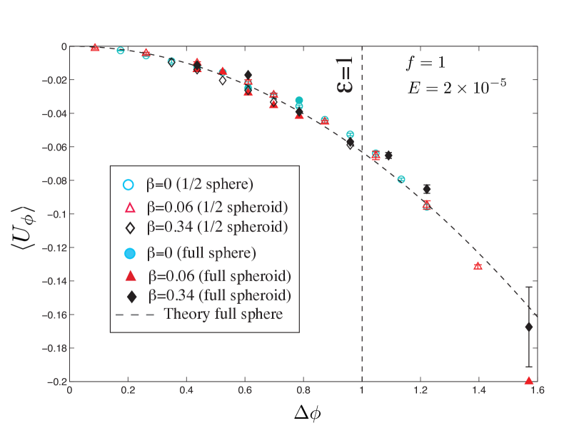
In Figure 6, we present the time averaged zonal flow from direct visualization and LDA measurements together for a fixed Ekman number, , a fixed libration frequency, , and a libration amplitude that varies from 0.05 to 1.6 rad. In all cases, the mean zonal flow is retrograde at the point of measurement. In the range of studied parameters and at the measurement location , we do not observe significant variations of the zonal flow amplitude with the ellipticity, nor with the half or full tank configurations. Hence, we expect the same mechanism, weakly dependent on the geometry, to produce the zonal flow in all 6 configurations (full tank, ; half tank ). Busse (2010, 2011); Calkins et al. (2010); Noir et al. (2010); Sauret et al. (2010); Sauret and Le Dizès (2012b) have proposed that the geostrophic zonal flow in librating axisymmetric containers results from boundary layer non-linear interactions, which yields a zonal flow independent of the Ekman number at the first order, scaling as . Sauret and Le Dizès (2012b) recover the pre-factor and the radial dependency of the geostrophic flow by deriving the boundary layer flow at the order in a full sphere (see Appendix). For a probe volume located at , same as dye injection location, and a frequency , the authors predicts a zonal flow, , with . We observe a good agreement between their analytical spherical model represented by the dashed line in Figure 6 and our LDA measurements in all 6 configurations up to rad. The theoretical zonal flow in a non-axisymmetric container has yet to be derived. Nevertheless, our results suggest that the full sphere model remains a good approximation at first order even for finite ellipticity, highlighting the minor role of the curvature in the source mechanism.
Significant deviations only appear for the largest value of studied here, where we observe a larger zonal flow than predicted by the non-linear analysis valid only for . It is likely that for , the boundary layer flow derivation of Sauret and Le Dizès (2012b) is not valid anymore and finite amplitude effects should be introduced.
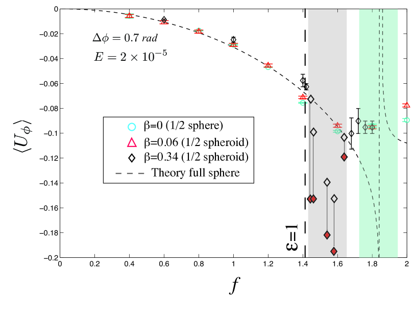
In Figure 7, we present LDA measurements of the time average zonal velocity as a function of the libration frequency at and a fixed libration amplitude rad. All measurements are performed only in the half container geometry using LDA to diagnose the flow. We also plot the analytical geostrophic zonal velocity for a probe volume located at derived from Sauret and Le Dizès (2012b) for a full sphere (see Appendix).
For and , we observe only marginal differences between the different half containers up to : the flow remains laminar and the experimental results are consistent with the retrograde geostrophic zonal flow predicted from the non-linear boundary layer mechanism. At higher frequencies, the theoretical analysis of Sauret and Le Dizès (2012b) predicts a geostrophic discontinuity in the zonal flow associated with the so-called critical latitude. As we scan in frequency, the geostrophic shear structure passes by the measurement point when , i.e. . In Figure 7, our LDA measurements do not show a sharp transition in this frequency range and we note a significant discrepancy between the predicted zonal flow and the time averaged velocity measurements. Several effects can account for this disagreement. First, in the theoretical analysis, the Ekman boundary layer becomes singular at the critical latitude resulting in a local infinite geostrophic shear. This discontinuity can be resolved by taking into account higher order terms. Doing so, the geostrophic shear has a finite amplitude and occurs in a width layer centered on the critical cylindrical radius (e.g. Noir et al., 2001; Kida, 2011). Thus, we do not expect the analytical zonal flow derived by Sauret and Le Dizès (2012b) to be valid when . As we scan in frequencies, the region of influence of the geostrophic shear stucture passes by the point of measurement located at a cylindrical radius when (Figure 7). Second, in this range of parameters becomes significantly larger than unity. Thus, we expect finite amplitude perturbations, not taken into account in the analytical model, to contribute to the local mean zonal velocity.
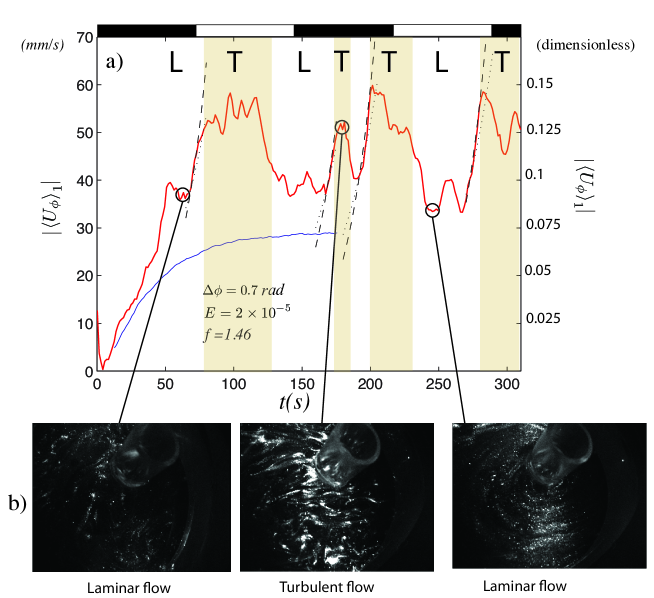
The case is more complex. Indeed, for , we observe intermittency of lower and higher amplitude zonal flows represented by open diamonds and red full diamonds, respectivey. This intermittency is illustrated in Figure 8, which represents the time evolution of the norm of the azimuthal velocity averaged over 10 oscillations for a particular experiment at rad (), , (red) and (blue). At , the zonal flow averaged over 10 oscillations evolves in time between a low amplitude and a large amplitude . Using a diluted Kalliroscope suspension and a camera at the top with a horizontal laser light sheet 1cm below the flat top lid we visualize the shear structures in the interior. Periods of large amplitude mean zonal flow are systematically correlated with small scale shear structures, corresponding to the bright filaments in the second snapshot, whereas periods of low amplitude mean zonal flow are associated with laminar flows, which are characterized by little contrast variation as on the first and last snapshots. The duration of each laminar and turbulent period varies over the experiment but is always of the order of a fraction of the spinup time (Each black and white rectangle at the top of Figure 8a represents a spinup time (s) ). The transition from low amplitude to large amplitude mean zonal flow occurs over a typical timescale s ( rotations) that remains consistent over the whole experiment. This particular dataset is representative of all experiments where intermittent turbulence is observed. The typical time scales of the herein reported intermittent turbulence are not consistent with the centrifugal instability observed in the spherical shell Noir et al. (2009) or in previous numerical simulations in non-axisymmetric ellipsoids at low libration frequencies by Chan et al. (2011), which both occur once per libration period.
In the band of frequency , the zonal flow predicted by Sauret and Le Dizès (2012b) is significantly different from our observations, in particular it fails at reproducing the intermittent low and large amplitude zonal flow.
5 Discussion and concluding remarks
In the present study we explore the zonal flow regimes driven by longitudinal libration in the ()-parameter space at for spherical and non-axisymmetric containers. At fixed frequency the flow in the bulk remains laminar for all accessible amplitudes of libration regardless of the tank geometry. In this laminar regime, we measure a net zonal flow that is independent of the geometry at first order and well explained by non-linearities in the Ekman boundary layer. In contrast, at a fixed amplitude of libration rad, we observe space-filling turbulence correlated with an enhanced zonal flow in specific bands of frequency and for the container with the largest equatorial ellipticity. Using two containers with different equatorial ellipticities and a spherical cavity, we unambiguously demonstrate that the observed instability results from the topographic coupling and not from viscously-driven dynamics. Although the range of accessible parameters in our device does not allow us to study in great details the mechanism underlying the onset of the turbulent regimes, some possible routes can be investigated.
Comparing Figure 6 and Figure 7 for , our results suggest that the onset of instability is not characterized by a critical Rossby number, . For no turbulence is observed in any of our containers even at the largest libration amplitude accessible in this experiment, which corresponds to a Rossby number . In contrast, the intermittent turbulence is observed in the container of large ellipticity in a band of frequency , corresponding to . This highlights the peculiar role of the ellipticity and frequency in the destabilization mechanism in the system.
In rapidly rotating non-axisymmetric container, intermittency of turbulent flows followed by a re-laminarization in particular bands of frequency are often typical of the growth and collapse of an elliptical instability (Malkus, 1989). Furthermore, recent numerical and theoretical work by Cébron et al. (2012) has demonstrated that longitudinal libration can drive elliptical instability in triaxial and biaxial ellipsoids. In order to test if such a mechanism could explain our observations we calculate the growth rate predicted by the geometry-independent WKB analysis Cébron et al. (2012):
| (14) |
with
| (15) |
where is resonant frequency and K is a viscous dissipation factor typically in the range . Assuming the base flow (13) is realized in the experiment and a perfect triadic resonance at , we obtain a negative growth rate for and a positive growth rate for . In Figure 8 we superimposed the theoretical growth of the azimuthal velocity for and the two extreme values of the dissipation factor, (dotted black) and (dashed black) to the time series of LDA azimuthal flow in the half spheroid configuration. The good agreement for , the most dissipative case, suggests that an LDEI mechanism may explain our observations. Note that the WKB approach is based on a local plane waves decomposition of the velocity field independent of the geometry of the container. It is therefore applicable to both the half and full container providing the same base flow is excited. The WKB analysis provides an upper bound of the growth rate. A more accurate prediction can be obtain via a global modes analysis, which is out of the scope of the present paper. In the present experiment, the limited quantitative diagnostics in this complex geometry do not allow us to draw a hard conclusion. Further numerical and experimental investigations at lower Ekman numbers will be necessary to characterize in details the mechanism underlying the intermittent turbulence and how this turbulence modifies the mean zonal flow. Exploring the parameter space using 3D numerical simulations in non-axisymmetric containers will remain limited to . We are currently developing a new experimental setup to overcome this limitation.
At planetary settings two scenarios may be drawn. In the first scenario, the conditions required to drive intermittent turbulence are not met and the topographic coupling does not significantly alter the dynamics driven by viscous interactions in the boundary layer. In that case we expect the flow in the interior to remain laminar with a time averaged zonal component independent of the Ekman number following a quadratic scaling in the amplitude of libration. This would lead insignificant zonal flows in the range m/day m/day for the celestial objects presented in table 2. As proposed by Calkins et al. (2010) such dynamics will not result in significant energy dissipation nor magnetic field generation. In the second scenario, topographically driven space-filling turbulence develop in the liquid layer of the planet. In that case one may expect significant energy dissipation and maybe magnetic field induction depending on the strength of the turbulence.
Understanding the underlying mechanism for the instability reported in the present study is therefore fundamental for planetary applications. In this study, we suggest that an LDEI mechanism, identified numerically by Cébron et al. (2012) in biaxial and triaxial librating ellipsoids, may be responsible for the observed space-filling turbulence at moderate Rossby numbers in our experiment.
Appendix: Analytical determination of the mean zonal flow
In this section, we present the main steps of the analytical derivation of the mean zonal flow induced by longitudinal libration in spherical geometry and we refer the reader to Sauret and Le Dizès (2012b) for a more complete and generic description.
In the limit of small Ekman number , the flow can be classically separated in two components: an inviscid component in the bulk and a viscous component in the Ekman boundary layer of size attached to the mantle. Using a perturbative approach in the limit of small libration amplitude , the flow can be written in the bulk:
| (16) |
and in the boundary layer
| (17) |
In the absence of librational forcing, the fluid is in solid-body rotation . Then, as long as the libration period remains small compare to the spin-up time, , no spinup takes place in the bulk at each libration cycle Busse (2010) and the first order correction of the bulk flow is null: . However, to adjust the velocity field between the bulk and the librating mantle, a flow oscillating at frequency develops in the thin Ekman layer. The nonlinear self-interactions of this oscillating flow lead to a nonlinear steady flow in the boundary layer at order , . The continuity of the velocity at the interface between the inviscid interior and the boundary layer implies a correction in the bulk flow at order , which generically writes . The expression of depends on the libration frequency and the specific shape of the container. The solution differs when considering a flat top boundary as in the cylindrical geometry Wang (1970) and a curved boundary as in the spherical geometry Sauret and Le Dizès (2012b).
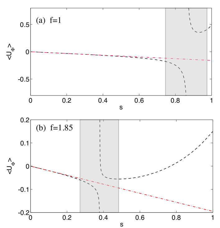
In figure 9, we show the resulting mean zonal flow as a function of the cylindrical radius for two libration frequencies and , in the case of a sphere and a cylinder. In all cases, we predict a scaling of the mean zonal flow with but the radial profiles are different in each geometry.
In the case of the sphere the asymptotic derivation predicts a divergent zonal flow at a critical cylindrical radius , which corresponds to the so-called critical latitude defined as Bondi and Lyttleton (1953):
| (18) |
| (19) |
This critical latitude is associated with a breakdown of the Ekman boundary layer due to the total absorption of the inertial waves at this location. In the analysis of Sauret and Le Dizès (2012b) this breakdown appears as a singularity,. However, including terms of order leads to a finite amplitude shear scaling as over a radial and latitudinal extension scaling as and , respectively Stewartson and Roberts (1963); Kida (2011). Using these scalings in the context of a precessional forcing, Noir et al. (2001); Kida (2011) have proposed that the geostrophic cylinder spawn by the critical latitude scales as in width and in amplitude. The breakdown of the Ekman boundary layer at the critical latitude and the subsequent scalings are generic to any oscillatory mechanical forcing through the boundary and remains therefore valid in the case of longitudinal libration Calkins et al. (2010). The complete derivation of the zonal flow including the higher order terms near the critical latitude is very fastidious and was beyond the scope of the analysis of Sauret and Le Dizès (2012b). Hence, we do not expect the theoretical profile derived from their analysis to apply in the range . At a fixed measurement point , when scanning in frequencies, the geostrophic shear alters the zonal flow measurements in a range (see Figure 7 in section 4).
Acknowledgements
The authors would like to thank F. H. Busse, S. Le Dizès, N. Rambaux, T. Van Hoolst and K. Zhang for fruitful discussions on the problem. This work was financially supported by NASA’s PG&G program (award #NNX09AE96G), PME program (award #NNX07AK44G) and ERC grant (247303 MFECE).
| Planets | Internal layer | (km) | (km) | (day) | (rad) | |||
|---|---|---|---|---|---|---|---|---|
| Callisto(1,2) | SO | 2300 | 2000-2300 | 16.68 | 1 | |||
| Ganymede(3,4) | LC | 800 | 0-500 | 7.15 | 1 | |||
| Earth’s moon(5) | LC | 350 | 0-150 | 27.3 | 1 | |||
| Titan(Grav) (6,7) | SO | 2500 | 2350-2450 | 15.95 | 1 | |||
| Mercury (8) | LC | 1800 | 0-1700 | 58.6 | 2/3 | (8) | ||
| Titan(Atm)(6,7) | SO | 2500 | 2350-2450 | 15.95 | (6) | |||
| Io(9) | LC | 500 | - | 1.77 | 1 | |||
| Europa(10) | SO | 1450 | 1300-1400 | 3.55 | 1 | (10) |
References
- Aldridge (1967) Aldridge, K. D., 1967. An experimental study of axisymmetric inertial oscillations of a rotating liquid sphere. Ph.D. thesis, Massachusetts Institute of Technology.
- Aldridge (1975) Aldridge, K. D., 1975. Inertial waves and Earth’s outer core. Geophysical Journal of the Royal Astronomical Society 42 (2), 337–345.
- Aldridge and Toomre (1969) Aldridge, K. D., Toomre, A., 1969. Axisymmetric inertial oscillations of a fluid in a rotating spherical container. Journal of Fluid Mechanics 37, 307–323.
- Anderson et al. (2001) Anderson, J. D., Jacobson, R. A., McElrath, T. P., Moore, W. B., Schubert, G., Thomas, P. C., 2001. Shape, mean radius, gravity field, and interior structure of Callisto. Icarus 153 (1), 157–161.
- Anderson et al. (1996) Anderson, J. D., Lau, E. L., Sjogren, W. L., Schubert, G., Moore, W. B., 1996. Gravitational constraints on the internal structure of Ganymede. Nature 384 (6609), 541–543.
- Anderson et al. (1998) Anderson, J. D., Schubert, G., Jacobson, R. A., Lau, E. L., Moore, W. B., Sjogren, W. L., 1998. Europa’s differentiated internal structure: Inferences from four galileo encounters. Science 281 (5385), 2019–2022.
- Bondi and Lyttleton (1953) Bondi, H., Lyttleton, R., 1953. On the dynamical theory of the rotation of the earth. ii. the effect of precession on the motion of the liquid core. Proc. Camb. Phil. Soc. 49, 498–515.
- Breuer et al. (2007) Breuer, D., Hauck, S. A., Buske, M., Pauer, M., Spohn, T., 2007. Interior evolution of Mercury. Space Science Reviews 132 (2-4), 229–260.
- Busse (2010) Busse, F., 2010. Mean zonal flows generated by librations of a rotating spherical cavity. Journal of Fluid Mechanics 650, 505–512.
- Busse (2011) Busse, F., 2011. Zonal flow induced by longitudinal librations of a rotating cylindrical cavity. Physica D: Nonlinear Phenomena 240, 208–211.
- Calkins et al. (2010) Calkins, M., Noir, J., Eldredge, J., Aurnou, J. M., 2010. Axisymmetric simulations of libration-driven fluid dynamics in a spherical shell geometry. Physics of Fluids 22, 1–12.
- Cebron et al. (2012) Cebron, D., Le Bars, M., Le Gal, P., 2012. Tidal instability in terrestrial planets and moons. A&A 539.
- Cébron et al. (2012) Cébron, D., Le Bars, M., Noir, J., Aurnou, J., 2012. Libration driven elliptical instability. Physics of Fluid, submitted.
- Chan et al. (2011) Chan, K., Liao, X., Zhang, K., 2011. Simulations of fluid motion in ellipsoidal planetary cores driven by longitudinal libration. Physics of the Earth and Planetary Interiors 187, 391–403.
- Comstock and Bills (2003) Comstock, R. L., Bills, B. G., 2003. A solar system survey of forced librations in longitude. Journal of Geophysical Research-Planets 108 (E9), 1–13.
- Goldreich and Mitchell (2010) Goldreich, P. M., Mitchell, J. L., 2010. Elastic ice shells of synchronous moons: Implications for cracks on Europa and non-synchronous rotation of Titan. Icarus 209 (2), 631–638.
- Hauck et al. (2006) Hauck, S. A., Aurnou, J. M., Dombard, A. J., 2006. Sulfur s impact on core evolution and magnetic field generation on Ganymede. Journal of Geophysical Research-Planets 111.
- Hauck et al. (2004) Hauck, S. A., Dombard, A. J., Phillips, R. J., Solomon, S. C., 2004. Internal and tectonic evolution of Mercury. Earth and Planetary Science Letters 222 (3-4), 713–728.
- Herreman et al. (2009) Herreman, W., Le Bars, M., Le Gal, P., 2009. On the effects of an imposed magnetic field on the elliptical instability in rotating spheroids. Phys. Fluids 21, 046602.
- Kerswell and Malkus (1998) Kerswell, R. R., Malkus, W. V. R., 1998. Tidal instability as the source for Io’s magnetic signature. Geophysical Research Letters 25 (5), 603–606.
- Kida (2011) Kida, S., 2011. Steady flow in a rapidly rotating sphere with weak precession. Journal of Fluid Mechanics 680, 150–193.
- Kuskov and Kronrod (2005) Kuskov, O., Kronrod, V., 2005. Internal structure of Europa and Callisto. Icarus 177, 550–569.
- Le Bars et al. (2010) Le Bars, M., Lacaze, L., Le Dizès, S., Le Gal, P., Rieutord, M., 2010. Tidal instability in stellar and planetary binary systems. Physics of the Earth and Planetary Interiors 178, 48–55.
- Le Bars et al. (2011) Le Bars, M., Wieczorek, M., Karatekin, Ö., Cébron, D., Laneuville, M., 2011. An impact-driven dynamo for the early moon. Nature 479, 215–218.
- Lorenz et al. (2008) Lorenz, R. D., Stiles, B. W., Kirk, R. L., Allison, M. D., Del Marmo, P. P., Iess, L., Lunine, J. I., Ostro, S. J., Hensley, S., 2008. Titan’s rotation reveals an internal ocean and changing zonal winds. Science 319 (5870), 1649–1651.
- Malkus (1989) Malkus, W., 1989. An experimental study of global instabilities due to tidal (elliptical) distortion of a rotating elastic cylinder. Geophys. Astrophys. Fluid Dyn. 48, 123.
- Margot et al. (2007) Margot, J. L., Peale, S. J., Jurgens, R. F., Slade, M. A., Holin, I. V., 2007. Large longitude libration of Mercury reveals a molten core. Science 316 (5825), 710–714.
- Noir et al. (2010) Noir, J., Calkins, M., Lasbleis, M., Cantwell, J., Aurnou, J. M., 2010. Experimental study of libration-driven zonal flows in a straight cylinder. Physics of the Earth and Planetary Interiors 182, 98–1106.
- Noir et al. (2009) Noir, J., Hemmerlin, F., Wicht, J., Baca, S., Aurnou, J. M., 2009. An experimental and numerical study of librationally driven flow in planetary cores and subsurface oceans. Physics of the Earth and Planetary Interiors 173, 141–152.
- Noir et al. (2001) Noir, J., Jault, D., Cardin, P., 2001. Numerical study of the motions within a slowly precessing sphere at low ekman number. Journal of Fluid Mechanics 437, 283–299.
- Sauret et al. (2012a) Sauret, A., Cébron, D., Le Bars, M., Le Dizès, S., 2012a. Fluid flows in librating cylinder. Physics of Fluids 24, 1–23.
- Sauret et al. (2010) Sauret, A., Cebron, D., Morize, C., Le Bars, M., 2010. Experimental and numerical study of mean zonal flows generated by librations of a rotating spherical cavity. Journal of Fluid Mechanics 662, 260–268.
- Sauret and Le Dizès (2012b) Sauret, A., Le Dizès, S., 2012b. Steady flow induced by longitudinal libration in a spherical shell. Journal of Fluid Mechanics, submitted.
- Sohl et al. (2002) Sohl, F., Spohn, T., Breuer, D., Nagel, K., 2002. Implications from galileo observations on the interior structure and chemistry of the galilean satellites. Icarus 157, 104–119.
- Spohn and Schubert (2003) Spohn, T., Schubert, G., 2003. Oceans in the icy galilean satellites of Jupiter? Icarus 161 (2), 456–467.
- Stewartson and Roberts (1963) Stewartson, K., Roberts, P. H., 1963. On the motion of a liquid in a spheroidal cavity of a precessing rigid body. Journal of Fluid Mechanics 17, 1–20.
- Tilgner (1999) Tilgner, A., 1999. Driven inertial oscillations in spherical shells. Physical Review E 59 (2), 1789–1794.
- Tobie et al. (2005) Tobie, G., Grasset, O., Lunine, J. I., Mocquet, A., Sotin, C., 2005. Titan’s internal structure inferred from a coupled thermal-orbital model. Icarus 175, 496–502.
- Van Hoolst et al. (2008) Van Hoolst, T. V., Rambaux, N., Karatekin, O., Dehant, V., Rivoldini, A., 2008. The librations, shape and icy shell of Europa. Icarus 195 (1), 386–399.
- Wang (1970) Wang, C., 1970. Cylindrical tank of fluid oscillating about a state of steady rotation. Journal of Fluid Mechanics 41, 581–592.
- Williams et al. (2001) Williams, J. G., Boggs, D. H., Yoder, C. F., Ratcliff, J. T., Dickey, J. O., 2001. Lunar rotational dissipation in solid body and molten core. Journal of Geophysical Research-Planets 106 (E11), 27933–27968.
- Williams and Dickey (2002) Williams, J. G., Dickey, J. O., 2002. Lunar geophysics, geodesy, and dynamics. In: 13th International Workshop on Laser Ranging. Washington, D. C.
- Williams et al. (2007) Williams, J. P., Aharonson, O., Nimmo, F., 2007. Powering Mercury’s dynamo. Geophysical Research Letters 34 (21).
- Yoder (1995) Yoder, C. F., 1995. Venus’ free obliquity. Icarus 117 (2), 250–286.
- Zhang et al. (2011) Zhang, K., Chan, K., Liao, X., 2011. On fluid motion in librating ellipsoids with moderate equatorial eccentricity. Journal of fluid mechanics 673, 468–479.