Crossover from Growing to Stationary Interfaces in the Kardar-Parisi-Zhang Class

Abstract

This Letter reports on how the interfaces in the (1+1)-dimensional Kardar-Parisi-Zhang (KPZ) class undergo, in the course of time, a transition from the flat, growing regime to the stationary one. Simulations of the polynuclear growth model and experiments on turbulent liquid crystal reveal universal functions of the KPZ class governing this transition, which connect the distribution and correlation functions for the growing and stationary regimes. This in particular shows how interfaces realized in experiments and simulations actually approach the stationary regime, which is never attained unless a stationary interface is artificially given as an initial condition.

Aside from their ubiquity in nature, surface growth phenomena constitute an important situation of statistical mechanics out of equilibrium, where scale invariance and universal scaling laws arise generically Barabási and Stanley (1995). These are usually evidenced in the roughness of the interfaces, whose amplitude $w(L,t)$ measured at the system (substrate) size $L$ and time $t$ obeys the following power laws:

$$w(L,t)\sim\begin{cases}L^{\alpha}&\text{for $L\ll{}L_{*}$,}\\ t^{\beta}&\text{for $L\gg{}L_{*}$,}\end{cases}\quad(L_{*}\sim t^{1/z}),$$ (1)

with scaling exponents $\alpha,\beta,z\equiv\alpha/\beta$ Family and Vicsek (1985); Barabási and Stanley (1995). At the heart of such growth processes is the Kardar-Parisi-Zhang (KPZ) equation Kardar et al. (1986) and the corresponding universality class Barabási and Stanley (1995); Kardar et al. (1986), describing the simplest case without any conservation laws and long-range interactions. For one-dimensional interfaces, the KPZ equation reads

$$\frac{\partial{}}{\partial{t}}h(x,t)=\nu\frac{\partial^{2}h}{\partial{x}^{2}}+\frac{\lambda}{2}\left(\frac{\partial{h}}{\partial{x}}\right)^{2}+\sqrt{D}\eta(x,t),$$ (2)

where $h(x,t)$ denotes the fluctuating height profile and $\eta(x,t)$ white Gaussian noise with $\langle{\eta(x,t)}\rangle=0$ and $\langle{\eta(x,t)\eta(x^{\prime},t^{\prime})}\rangle=\delta(x-x^{\prime})\delta(t-t^{\prime})$. The values of the scaling exponents are exactly known in this one-dimensional case Barabási and Stanley (1995); Kardar et al. (1986); Forster et al. (1977): the height fluctuation $\delta{}h\equiv{}h-\langle{h}\rangle$ grows as $\delta{}h\sim{}t^{1/3}$ ($\beta=1/3$) and the correlation length $\xi$ as $\xi\sim{}t^{2/3}$ ($z=3/2$). Specifically, $h$ is described by a rescaled random variable $\chi(x^{\prime},t)$ as

$$h(x,t)\simeq v_{\infty}t+(\Gamma t)^{1/3}\chi(x^{\prime},t)$$ (3)

with a rescaled coordinate $x^{\prime}\equiv(Ax/2)(\Gamma{}t)^{-2/3}$ and constant parameters $A\equiv\nu/2D,\Gamma\equiv{}A^{2}\lambda/2$, and $v_{\infty}$. The KPZ-class exponents have indeed been reported in various models and theoretical situations Barabási and Stanley (1995); Kardar et al. (1986); Forster et al. (1977); [Forrecentreviews; see; e.g.; ]Kriecherbauer.Krug-JPA2010; *Sasamoto.Spohn-JSM2010; *Corwin-RMTA2012 as well as by a growing number of experiments Wakita et al. (1997); Maunuksela et al. (1997); *Myllys.etal-PRE2001; Takeuchi and Sano (2010); *Takeuchi.etal-SR2011; Takeuchi and Sano (2012); Huergo et al. (2010); *Huergo.etal-PRE2011; Yunker et al. (2013); Aegerter et al. (2003).

Studies on the (1+1)-dimensional KPZ class entered an unprecedented stage in 2000, when Johansson Johansson (2000) and others Kriecherbauer and Krug (2010) rigorously derived asymptotic distributions of the height fluctuations for a few models. Among others, it has brought about two outstanding outcomes. (i) The KPZ class splits into a few subclasses according to the global geometry of the interfaces, or, equivalently, to the initial condition. These subclasses are characterized by different distribution and correlation functions, whereas they share the same scaling exponents. (ii) An unexpected link to random matrix theory has been revealed. In particular, the asymptotic distribution of $\chi$ for the flat and curved interfaces is given by the largest-eigenvalue distribution, called the Tracy-Widom (TW) distribution Tracy and Widom (1994); *Tracy.Widom-CMP1996; Mehta (2004), for the Gaussian orthogonal ensemble (GOE) and the Gaussian unitary ensemble, respectively Prähofer and Spohn (2000). The stationary interfaces also form a distinct subclass. To study it analytically, one usually sets the initial condition $h(x,0)$ to be a stationary interface, which is simply the one-dimensional Brownian motion for the KPZ equation Barabási and Stanley (1995). The height difference $h(x,t)-h(x,0)$ then grows as Eq. (3) and $\chi$ obeys the $F_{0}$ distribution introduced by Baik and Rains Baik and Rains (2000), as proved for the polynuclear growth (PNG) model Baik and Rains (2000); Prähofer and Spohn (2000), for the totally asymmetric simple exclusion process Ferrari and Spohn (2006); Baik et al. (2012), and, very recently, for the KPZ equation Imamura and Sasamoto (2012); *Imamura.Sasamoto-JSP2013. The two-point correlation function being exactly derived as well Prähofer and Spohn (2004); Ferrari and Spohn (2006); Baik et al. (2010, 2012); Imamura and Sasamoto (2012), this subclass is now firmly established like the ones for the flat and curved interfaces.

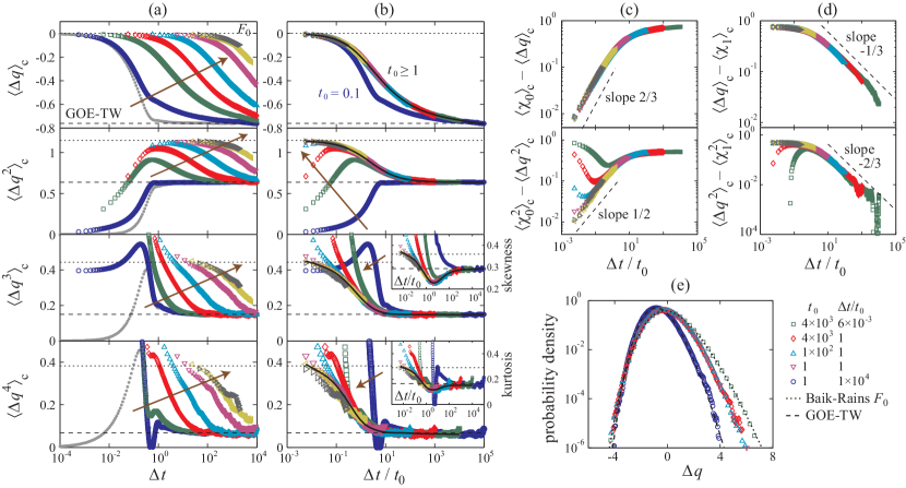
Figure 1: (color online). Crossover in the one-point distribution for the PNG model. (a,b) First- to fourth-order cumulants $\langle{\Delta{}q^{n}}\rangle_{\mathrm{c}}$ against $\Delta{}t$ (a) and $\Delta{}t/t_{0}$ (b), for $t_{0}=0,0.1,1,10,100,1000,4000,7000$ (increasing as the arrows indicate). The top (dotted) and bottom (dashed) horizontal lines indicate the values for the Baik-Rains $F_{0}$ and GOE-TW distributions, $\langle{\chi_{0}^{n}}\rangle_{\mathrm{c}}$ and $\langle{\chi_{1}^{n}}\rangle_{\mathrm{c}}$, respectively. The black solid lines in (b) show fitting to the collapsed curves (see text). The insets in (b) show the skewness and the kurtosis. (c,d) Asymptotic behavior of the data in (b) for small and large $\Delta{}t/t_{0}$. The data for $t_{0}=0.1$ are omitted because of the strong finite-time effect. (e) Distribution of $\Delta{}q$ for given pairs of $t_{0}$ and $\Delta{}t/t_{0}$.

Such a stationary regime is, however, never attained within a finite time in an infinitely large system, unless a stationary interface is artificially given as an initial condition. This is readily seen by recalling that the correlation length grows as $\xi\sim{}t^{2/3}$, whereas it is infinite for the stationary interfaces. Therefore, in practical situations starting from a smooth or uncontrolled initial profile, one needs to elucidate how the interfaces approach the stationary regime in the course of time. This is achieved by the present Letter. Simulations of the PNG model show that the height difference of the flat interfaces exhibits a transition from the flat, growing regime to the stationary one. We find scaling functions describing this crossover and determine their functional forms, which smoothly connect the GOE-TW and Baik-Rains $F_{0}$ distributions. We also study the two-point correlation function and show how those for the two subclasses interplay at finite times. These results are quantitatively reproduced by experimental data on turbulent liquid crystal Takeuchi and Sano (2010); *Takeuchi.etal-SR2011; Takeuchi and Sano (2012), indicating that they are universal characteristics of the KPZ-class interfaces.

First we study the PNG model. Starting from a flat substrate $h(x,0)=0$, an interface experiences random nucleation events at a uniform rate. On each nucleation, the local height $h(x,t)$ increases by one, producing a plateau that expands laterally at constant speed. When two plateaux encounter, they simply coalesce. For the simulations in continuous space and time, we numerically implement space-time representation used for analytical derivation of the distribution function Baik and Rains (2000); Prähofer and Spohn (2000), with the nucleation rate 2 per unit space and time and the plateau expansion speed 1. This choice of the parameters corresponds to $v_{\infty}=2,A=2$, and $\Gamma=1$. We impose the periodic boundary condition with system size $L=10^{3}$ and realize $10^{4}$ independent interfaces up to time $10^{4}$. The size is chosen to satisfy $L\gg{}L_{*}$ until $t=10^{4}$ [Eq. (1)] so that the system does not reach the saturated regime, which is not the crossover addressed in this Letter.

The quantity of interest is the height difference $\Delta{}h(x,\Delta{}t,t_{0})\equiv{}h(x,t_{0}+\Delta{}t)-h(x,t_{0})$, rescaled here as

$$\Delta q(x,\Delta t,t_{0})\equiv\frac{\Delta h-v_{\infty}\Delta t}{(\Gamma\Delta t)^{1/3}}.$$ (4)

By construction, $\Delta{}q\stackrel{{\scriptstyle\mathrm{d}}}{{\to}}\chi_{1}$ for $t_{0}\to 0$ and then $\Delta{}t\to\infty$, while $\Delta{}q\stackrel{{\scriptstyle\mathrm{d}}}{{\to}}\chi_{0}$ for $t_{0}\to\infty$ and then $\Delta{}t\to\infty$, where $\chi_{1}$ and $\chi_{0}$ are random variables obeying the GOE-TW and Baik-Rains $F_{0}$ distributions, respectively, with the factor $2^{-2/3}$ multiplied with the usual definition for the former Baik and Rains (2000); Prähofer and Spohn (2000). Figure 1(a) shows the first- to fourth-order cumulants of $\Delta{}q$, $\langle{\Delta{}q^{n}}\rangle_{\mathrm{c}}$, as functions of $\Delta{}t$ for different $t_{0}$, displayed with the values for the GOE-TW and Baik-Rains $F_{0}$ distributions (dashed and dotted lines, respectively). The cumulants agree with those for the GOE-TW distribution as $\Delta{}t$ tends to infinity, while they indicate the values of the Baik-Rains $F_{0}$ distribution for large $t_{0}$ and small enough $\Delta{}t$. The transition curves are found to collapse very well when $\Delta{}t$ is scaled by $t_{0}$ [Fig. 1(b)], except for too small $t_{0}$ and $\Delta{}t$. In particular, for $t_{0}\to\infty$, the cumulants converge to a single set of functions, $\langle{\Delta{}q^{n}}\rangle_{\mathrm{c}}\to\Delta{}Q_{n}(\Delta{}t/t_{0})$, satisfying $\Delta{}Q_{n}(\tau)\to\langle{\chi_{1}^{n}}\rangle_{\mathrm{c}}$ for $\tau\to\infty$ and $\Delta{}Q_{n}(\tau)\to\langle{\chi_{0}^{n}}\rangle_{\mathrm{c}}$ for $\tau\to 0$. One can indeed draw the functions $\Delta{}Q_{n}(\tau)$ by making histograms for $\langle{\Delta{}q^{n}}\rangle_{\mathrm{c}}$ at each $\Delta{}t/t_{0}$ with varying $t_{0}$ and fitting their modes by, e.g., spline functions, as shown by the black solid lines in Fig. 1(b). Theoretical expressions of $\Delta{}Q_{n}(\tau)$ are unknown, because they involve time correlation which still remains analytically unsolved. Asymptotically, the data suggest $\langle{\chi_{0}}\rangle_{\mathrm{c}}-\Delta{}Q_{1}(\tau)\sim\tau^{2/3}$, $\langle{\chi_{0}^{2}}\rangle_{\mathrm{c}}-\Delta{}Q_{2}(\tau)\sim\tau^{1/2}$ for small $\tau$ and $\Delta{}Q_{1}(\tau)-\langle{\chi_{1}}\rangle_{\mathrm{c}}\sim\tau^{-1/3}$, $\Delta{}Q_{2}(\tau)-\langle{\chi_{1}^{2}}\rangle_{\mathrm{c}}\sim\tau^{-2/3}$ for large $\tau$ [Fig. 1(c,d)]. While this convergence to the GOE-TW distribution ($\tau\to\infty$) is analogous to that of the height variable $h(x,t)$ Ferrari and Frings (2011); Oliveira et al. (2012); Takeuchi and Sano (2012), the power laws toward the Baik-Rains $F_{0}$ distribution ($\tau\to 0$) indicate unusual exponents that need to be explained theoretically. For higher orders $n\geq 3$, one needs better statistical accuracy to determine the asymptotics. In between the two limits, the transition occurs earlier for larger $n$ ($\leq 4$), leading to interesting undershoot in the skewness $\langle{\Delta{}q^{3}}\rangle_{\mathrm{c}}/\langle{\Delta{}q^{2}}\rangle_{\mathrm{c}}^{3/2}$ and the kurtosis $\langle{\Delta{}q^{4}}\rangle_{\mathrm{c}}/\langle{\Delta{}q^{2}}\rangle_{\mathrm{c}}^{2}$ [insets of Fig. 1(b)]. Finally, this crossover can also be checked directly in the distribution; Fig. 1(e) shows that the probability density functions of $\Delta{}q$ overlap for fixed $\Delta{}t/t_{0}$, and that they shift from the Baik-Rains $F_{0}$ to the GOE-TW distributions as $\Delta{}t/t_{0}$ is increased.

Now we turn our attention to the two-point correlation function, defined here by

$$C(l,\Delta t,t_{0})\equiv\left\langle{[\delta h(x+l,t_{0}+\Delta t)-\delta h(x,t_{0})]^{2}}\right\rangle$$ (5)

with $\delta{}h(x,t)\equiv{}h(x,t)-\langle{h(x,t)}\rangle$. If one takes the stationary limit $t_{0}\to\infty$ and then considers large $\Delta{}t$, one has $C^{\prime}(\zeta,\Delta{}t,t_{0})\equiv(\Gamma\Delta{}t)^{-2/3}C(l,\Delta{}t,t_{0})\simeq g(\zeta)$ with rescaled length $\zeta\equiv(Al/2)(\Gamma\Delta{}t)^{-2/3}$, where $g(\zeta)$ is the exact solution for the rescaled stationary correlation Prähofer and Spohn (2004); Imamura and Sasamoto (2012). This is tested in Fig. 2(a) with finite $t_{0}$ and $\Delta{}t$, where $\Delta{}C^{\prime}(\zeta,\Delta{}t,t_{0})\equiv{}C^{\prime}(\zeta,\Delta{}t,t_{0})-C^{\prime}(0,\Delta{}t,t_{0})$ is compared with $g(\zeta)-g(0)$ in the main panel. First we note that the data for fixed $\Delta{}t/t_{0}$ and different $t_{0}$ overlap with each other, confirming that $\Delta{}t/t_{0}$ is the only time scale that controls the dynamics. Now, we focus on the data with the smallest $\Delta{}t/t_{0}$ we have, namely $\Delta{}t/t_{0}=0.006$, shown by solid symbols in Fig. 2(a) (top data set). They are found to indicate the stationary correlation function for small $\zeta$, with or without subtraction of $C^{\prime}(0,\Delta{}t,t_{0})$ (main panel and inset, respectively). By contrast, for large $\zeta$, the correlation is governed by the spatial correlation of the flat interfaces, namely the Airy₁ correlation $g_{1}(\cdot)$, defined by $g_{1}(v)\equiv\langle{\mathcal{A}_{1}(u+v)\mathcal{A}_{1}(u)}\rangle-\langle{\mathcal{A}_{1}(u)}\rangle^{2}$ with the Airy₁ process $\mathcal{A}_{1}(u)$ Sasamoto (2005); Borodin et al. (2008); Not . To see this, we take $\Delta{}t\to 0$ in Eq. (5) and obtain, for large $t_{0}$, $\Delta{}C^{\prime}(\zeta,0,t_{0})=C^{\prime}(\zeta,0,t_{0})\simeq 2(\Delta{}t/t_{0})^{-2/3}\left[g_{1}(0)-g_{1}\left((\Delta{}t/t_{0})^{2/3}\zeta\right)\right]$. This function with $\Delta{}t/t_{0}=0.006$ is indicated by the dotted line in Fig. 2(a) and accounts for the data with large $\zeta$. In short, when $\Delta{}t/t_{0}$ is small enough,

$$C^{\prime}(\zeta,\Delta t,t_{0})\!\simeq\!\begin{cases}g(\zeta)&\!\!(\zeta\ll\zeta_{\mathrm{c}}),\\ \!2(\tfrac{\Delta t}{t_{0}})^{-\tfrac{2}{3}}\!\left[g_{1}(0)\!-\!g_{1}\!\left(\!\!(\tfrac{\Delta t}{t_{0}})^{\tfrac{2}{3}}\zeta\!\right)\right]&\!\!(\zeta\gg\zeta_{\mathrm{c}}),\end{cases}$$ (6)

where the crossover length $\zeta_{\mathrm{c}}$ is defined by the intersection of the two functions. If $\Delta{}t/t_{0}$ is further decreased in Fig. 2(a), the Airy₁ branch moves away as $(\Delta{}t/t_{0})^{-2/3}$ along both axes, leaving, asymptotically, only the stationary correlation $g(\zeta)$ as expected. Alternatively, if $C$ and $l$ are rescaled by $t_{0}^{2/3}$ instead of $\Delta{}t^{2/3}$, what remains asymptotically is the Airy₁ correlation. For tiny but finite $\Delta{}t/t_{0}$, the two branches are connected by $C^{\prime}\simeq 2\zeta$.

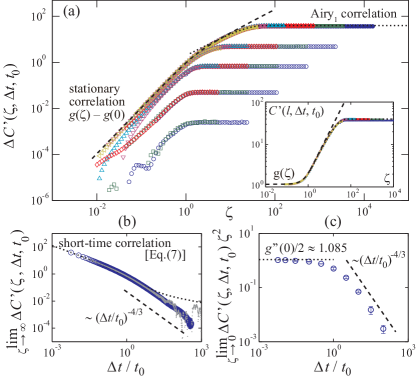
Figure 2: (color online). Crossover in the correlation function for the PNG model. (a) $\Delta{}C^{\prime}(\zeta,\Delta{}t,t_{0})$ against $\zeta$ for $\Delta{}t/t_{0}=0.006,0.1,1,10,100$ (different sets of data; increasing from top to bottom) and $t_{0}=1,10,100,1000,4000,7000$ (different colors and symbols; increasing from right to left). The dashed and dotted lines indicate the stationary correlation and the Airy₁ correlation as described in Eq. (6), respectively, with $\Delta{}t/t_{0}=0.006$ for the latter. The inset shows the data for $\Delta{}t/t_{0}=0.006$ without subtraction of $C^{\prime}(0,\Delta{}t,t_{0})$. (b,c) Asymptotics of $\Delta{}C^{\prime}(\zeta,\Delta{}t,t_{0})$ for $\zeta\to\infty$ (b) and $\zeta\to 0$ (c). Blue circles are the numerical estimates, obtained from the data with $t_{0}=10$ for (b) and with various $t_{0}$ for (c). The gray dots in (b) show the values of the right-hand side of Eq. (9), where $\langle{\Delta{}q^{2}}\rangle_{\mathrm{c}}$ for $t_{0}=10$ and $100$ is used as $Q_{2}(\tau)$.

We then study how the correlation function varies for large $\Delta{}t/t_{0}$. The data series in Fig. 2(a) show that $\Delta{}C^{\prime}(\zeta,\Delta{}t,t_{0})$ decreases with increasing $\Delta{}t/t_{0}$. In the limit $\zeta\to\infty$, since $\langle{\delta{}h(x+l,t_{0}+\Delta{}t)\delta{}h(x,t_{0})}\rangle\to 0$, we have $\Delta{}C^{\prime}(\zeta,\Delta{}t,t_{0})\to 2(\Gamma\Delta{}t)^{-2/3}C_{\mathrm{t}}(\Delta{}t,t_{0})$ with $C_{\mathrm{t}}(\Delta{}t,t_{0})\equiv\langle{\delta{}h(x,t_{0}+\Delta{}t)\delta{}h(x,t_{0})}\rangle$, i.e., the time correlation function. Despite the lack of analytical solution, its short-time behavior ($\Delta{}t/t_{0}\ll 1$) is given by

$$C_{\mathrm{t}}(\Delta t,t_{0})\simeq(\Gamma^{2}t_{0}t_{\mathrm{r}})^{\tfrac{1}{3}}\langle{\chi_{1}^{2}}\rangle_{c}\biggl{[}1-\frac{\langle{\chi_{0}^{2}}\rangle_{c}}{2\langle{\chi_{1}^{2}}\rangle_{c}}\!\left(1-\frac{t_{0}}{t_{\mathrm{r}}}\right)^{\!\!\tfrac{2}{3}}\biggr{]}$$ (7)

with $t_{\mathrm{r}}\equiv{}t_{0}+\Delta{}t$ Krug et al. (1992); Kallabis and Krug (1999); Takeuchi and Sano (2012). For $\Delta{}t/t_{0}\gg 1$, numerical Kallabis and Krug (1999) and experimental Takeuchi and Sano (2012) studies showed $C_{\mathrm{t}}(\Delta{}t,t_{0})\simeq(\Gamma^{2}t_{0}t_{\mathrm{r}})^{1/3}F(\Delta{}t/t_{0})$ with $F(\tau)\sim\tau^{-1}$. They indicate

$$\lim_{\zeta\to\infty}\!\Delta C^{\prime}(\zeta,\Delta t,t_{0})\sim\begin{cases}(\Delta t/t_{0})^{-2/3},&\!(\Delta t/t_{0}\ll 1),\\ (\Delta t/t_{0})^{-4/3},&\!(\Delta t/t_{0}\gg 1),\end{cases}$$ (8)

and correctly account for the data [Fig. 2(b)]. Further, since the second-order cumulant of the rescaled height difference, $Q_{2}(\Delta{}t/t_{0})$, involves the two-point time correlation $C_{\mathrm{t}}(\Delta{}t,t_{0})$, we also obtain for arbitrary $\Delta{}t/t_{0}$

$$\lim_{\zeta\to\infty}\Delta C^{\prime}(\zeta,\Delta t,t_{0})$$

$$=\langle{\chi_{1}^{2}}\rangle_{c}\biggl{[}\!\left(1+\frac{1}{\Delta t/t_{0}}\right)^{\!\!\tfrac{2}{3}}\!\!+(\Delta t/t_{0})^{-\tfrac{2}{3}}\biggr{]}\!-Q_{2}(\Delta t/t_{0}).$$ (9)

This is also confirmed as shown by gray dots in Fig. 2(b).

In contrast to the long-length limit, one cannot a priori predict how the short-length limit $\zeta\to 0$ of $\Delta{}C^{\prime}(\zeta,\Delta{}t,t_{0})$ depends on $\Delta{}t/t_{0}$. The data in Fig. 2(a) suggest $\Delta{}C^{\prime}(\zeta,\Delta{}t,t_{0})\sim\zeta^{2}$ for any $\Delta{}t/t_{0}$. Figure 2(c) shows that the coefficient of this quadratic term varies as

$$\lim_{\zeta\to 0}\Delta C^{\prime}(\zeta,\Delta t,t_{0})\zeta^{-2}=\frac{1}{2}\left.\frac{\partial^{2}C^{\prime}}{\partial{\zeta}^{2}}\right|_{\zeta=0}$$

$$\qquad\qquad\simeq\begin{cases}g^{\prime\prime}(0)/2\approx 1.085&(\Delta t/t_{0}\ll 1),\\ c(\Delta t/t_{0})^{-4/3}&(\Delta t/t_{0}\gg 1),\end{cases}$$ (10)

with a constant $c$ and the second derivative $g^{\prime\prime}(0)$, which naturally arises since $C^{\prime}(\zeta,\Delta{}t,t_{0})\to{}g(\zeta)$ for $\Delta{}t/t_{0}\to 0$. To examine the other limit, let us note $\frac{1}{2}\left.\frac{\partial^{2}C^{\prime}}{\partial\zeta^{2}}\right|_{\zeta=0}=(A/2)^{-2}(\Gamma\Delta{}t)^{2/3}\langle{\frac{\partial{h}}{\partial{x}}(x,t_{0}+\Delta{}t)\frac{\partial{h}}{\partial{x}}(x,t_{0})}\rangle$, which is simply time correlation in the slope of the interface. It is suggestive that the short- and long-length limits of $\Delta{}C^{\prime}(\zeta,\Delta{}t,t_{0})$ are governed by the slope-slope and height-height time correlations, respectively, decaying with the same power in the rescaled units [Eqs. (8) and (10)]. The results may also remind us of the space-like and time-like paths argued in the literature Ferrari (2008); Corwin et al. (2012), though precise relation is yet to be clarified.

Finally, we test universality of the presented crossover, analyzing experimental data of growing interfaces in turbulent liquid crystal. While the readers are referred to Refs. Takeuchi and Sano (2010, 2012) for detailed descriptions, in this series of work the author and a coworker studied planar evolution of borders between two distinct regimes of spatiotemporal chaos, called the dynamic scattering modes 1 and 2, in the electroconvection of nematic liquid crystal. The interfaces grow under high applied voltage, clearly exhibiting, besides the exponents, the distribution and correlation functions for the flat and curved KPZ-class interfaces Takeuchi and Sano (2010, 2012). Here, we employ the data for 1128 flat interfaces used in Ref. Takeuchi and Sano (2012) and perform the crossover analyses developed in the present study.

Figure 3: (color online). Crossover in the liquid-crystal experiment. (a,b) Cumulants (a) and skewness (b) against $\Delta{}t/t_{0}$ with $t_{0}=2,6,10,18,30,54,60~{}\mathrm{s}$ (from right to left). The inset shows $\langle{\Delta{}q}\rangle_{\mathrm{c}}$ against $\Delta{}t$. The dotted and dashed lines indicate the values for the Baik-Rains $F_{0}$ and GOE-TW distributions, respectively. The solid curves show the fitting to the PNG data obtained in Fig. 1(b). (c) Rescaled correlation function $\Delta{}C^{\prime}(\zeta,\Delta{}t,t_{0})$ against $\zeta$ for given $t_{0}$ and $\Delta{}t/t_{0}$ ($\Delta{}t/t_{0}$ increases from top to bottom). The red dashed and black dotted lines indicate the stationary and Airy₁ correlation functions as described in Eq. (6), respectively, the latter being set with $\Delta{}t/t_{0}=0.006$. The three black solid lines trace PNG data in Fig. 2(a) with corresponding values of $\Delta{}t/t_{0}$.

Figure 3 shows the results. The $n$th-order cumulants of the rescaled height difference $\Delta{}q$ [Eq. (4)] with various $t_{0}$, which sufficiently fall apart as functions of $\Delta{}t$ [see, e.g., inset of Fig. 3(a)], collapse reasonably well when plotted against $\Delta{}t/t_{0}$ [Fig. 3(a)], despite a rather strong finite-time effect for $n\geq 2$. The collapsed data are found asymptotically on top of the fitting curves obtained for the PNG model, $Q_{n}(\Delta{}t/t_{0})$ (black solid lines). This implies that $Q_{n}(\tau)$ are universal functions of the KPZ class describing the crossover in question, and so is the distribution function of $\Delta{}q$ parametrized by $\Delta{}t/t_{0}$. The undershoot in the skewness is also confirmed experimentally [Fig. 3(b)], while it was not clearly identified for the kurtosis because of larger statistical error (not shown). Moreover, extrapolation of the finite-time corrections in the cumulants allows us to roughly estimate the time needed for direct observation of the Baik-Rains $F_{0}$ distribution, longer than $10^{3}~{}\mathrm{s}$ here, which is unfortunately unreachable in the current setup Takeuchi and Sano (2010, 2012).

The results on the correlation function are also reproduced experimentally [Fig. 3(c)]. The functional form is parametrized solely by $\Delta{}t/t_{0}$ (see two data sets for $\Delta{}t/t_{0}=10^{-1}$ overlapping with each other) and agrees very well with the one obtained for the PNG model (black solid lines). In particular, the crossover between the stationary and Airy₁ correlations [Eq. (6)] is clearly confirmed for small enough $\Delta{}t/t_{0}$ (top yellow data set).

In summary, we have studied the flat-stationary crossover in the KPZ class, which takes place gradually in time. Analyzing numerical and experimental data, we have found and determined universal functions describing the cumulants and the two-point correlation during this crossover. These functions show multifaceted relations to the analytically unsolved time correlation, and hence may provide an important clue toward its solution. Seeking a possible connection to analogous, mathematically tractable crossover in space Corwin (2012) is another interesting issue left for future studies. Besides such fundamental importance, our results also answer a practical question of how interfaces realized in experiments and simulations approach the stationary regime, which is never attained without full control on the initial condition.