Connecting the Dots: Computer Systems Education
using a Functional Hardware Description Language

Abstract

A functional hardware description language enables students to gain a working understanding of computer systems, and to see how the levels of abstraction fit together. By simulating circuits, digital design becomes a living topic, like programming, and not just a set of inert facts to memorise. Experiences gained from more than 20 years of teaching computer systems via functional programming are discussed.

1 Introduction

Since 1991, a variety of courses on computer systems in the Department (now the School) of Computing Science at the University of Glasgow have been presented by the author using a functional hardware description language. Approximately 35 one-semester courses over 20 years have used these methods. The language is called Hydra, and is currently implemented by embedding in Haskell. Development of the approach to teaching computer systems and research on the Hydra language have interacted strongly, and each has influenced the other. A paper discussing how an earlier version of Hydra was used in teaching computer architecture appeared in 1995 [6]. This paper gives an overview of the current approach, which has evolved significantly since then, and discusses the experience that has been gained.

A sign of maturity of functional programming is its quiet application to practical problem domains, including education, without too much emphasis on the functional language itself. The focus in this paper is on the challenges in understanding computer systems, and how these challenges can be met successfully. The emphasis is on the subject area, not on the language. A thesis of this paper, however, is that the aims of teaching computer hardware are supported very well by a functional hardware description language, and rather poorly by traditional imperative ones. The final result is not a claim that “functional is better”, but simply that students gain a deeper insight into computer systems.

Section 2 discusses the rationale behind this approach to teaching computer systems, and Section 3 summarises the main topics covered. It is crucial to be explicit about circuit models, for reasons discussed in Section 4. Section 5 briefly describes the Hydra hardware description language, while Section 6 gives some examples. Section 7 discusses opportunities for incorporating formal methods in hardware design, and Section 8 outlines several exercises that have been used in recent years. Section 9 discusses a number of observations gained through years of experience teaching computer systems with functional programming, and Section 10 draws some conclusions.

2 Rationale

Computer science education has traditionally focused on programming and software development. It is common to provide some courses on computer systems, including an introduction to digital circuit design and computer architecture, but these courses often lack the depth found in software engineering. Standard topics include an introduction to digital circuits, instruction set architecture, and basic processor organisation.

A major problem with typical courses on computer hardware is a failure to “connect the dots”: various details of each level of abstraction are covered, but the crucial connections between the levels are largely ignored. To understand computer systems properly, it is necessary to have a working understanding of each level of abstraction, and also to understand the connections between the levels. To achieve this goal, it is essential to select the topics to be covered in each level carefully, so the techniques presented in one level are sufficient for supporting the next level up.

What is meant here by a “working understanding” goes beyond just knowing a collection of facts (the names of the registers, the names of the techniques, the names of the events that occur). A working understanding implies the ability to hand-execute the system, as well as to design parts or all of it, and to modify it. A working understanding provides the foundation for quantitative assessment of performance.

In contrast, many courses and textbooks (e.g. [9]) on computer systems describe the hardware with schematic diagrams, but do not provide a working understanding. This is reflected in many textbook problems that ask for descriptive answers that can be culled from the text.

Here is an example of what a working understanding means. There is a technique in processor design called bypassing, which can speed up a processor by eliminating pipeline stalls and thus increasing the amount of parallelism that is achievable. Many textbooks describe bypassing, sometimes in considerable detail, but it is easy to puncture the veneer of a student’s understanding by asking some probing questions: Here is a fragment of machine code; how many clock cycles faster will it run with bypassing? Modify a processor to implement bypassing (i.e. design absolutely every logic gate and signal needed to do it). What performance penalty, if any, is introduced by bypassing? Unfortunately, there is not room in this paper to provide a working understanding of bypassing, but it can be done in a 20-lecture course using a powerful hardware description language—and Hydra is ideal for this purpose.

Consider a thought experiment. What if computer programming and software engineering were taught descriptively? There would be explanations of what it’s like to write a program, discussions of how to organise your thinking, and of course a mass of UML diagrams. But suppose the students never write a program, and never hand-execute any code. The obvious objection is that they would not be able to do real-world programming after such an education. But a further objection is that the students would not have a working understanding of programming: they would not understand conceptually what a computer is doing. (There are indeed some courses like this, with titles like “Computing for Poets”, but they are intended for non-computing students.)

For many computer science students, hardware topics are taught descriptively, and the students fail to gain a working understanding. Two reasons for this are:

• Computer systems are complex, with many levels of abstraction, and each level is a large subject on its own. There isn’t enough time to cover all this material.

• Hardware is seen as an ancillary topic; it’s just there to run software, which is the important part of computing. According to a cliche, computer science is not about computers, so presumably there is no need to find out how they work.

A response to these problems is:

• Although systems are complex, it isn’t necessary to cover all the details of all the levels. With suitable notation (this is where the functional language enters), the essential details can be covered clearly and concisely, providing a working understanding. In addition, we can achieve a working understanding of how each level of abstraction connects to the levels above and below it. However, it is necessary to present the right concepts at each level. If we cover precisely the techniques needed to support the next level up, then we can explain the connection precisely. Sadly, many courses and textbooks cover a random selection of topics at each level, while ignoring the topics that are needed to connect the levels.

• Hardware is just as much about algorithms as software is. There is indeed a distinction between hardware and software, but there are also profound similarities. Students often do not perceive these similarities, and this is partly the result of ineffective languages for describing the hardware, which unnecessarily obscure the algorithmic content of the hardware.

We would not have computer science without computers, and surely it is reasonable for any educated computing professional to have a good working understanding of how a processor executes programs. Fortunately, this does not require excessive learning time.

Several courses and supporting textbooks follow a similar philosophy, using software tools and careful selection of topics to enable the main ideas in computer systems to be connected with each other. A book by Nisan and Schocken [5], supported by software tools, introduces circuits, architecture, and systems software at an elementary level. A book by Harris and Harris [3] covers circuit design and processor architecture at a more advanced level, and uses standard imperative hardware description languages (SystemVerilog and VHDL) to present a MIPS processor.

3 Course topics

Glasgow has a four-year undergraduate honours degree, as well as 1-year taught postgraduate MSc degrees. Over the years, the author has taught courses on computer systems at undergraduate levels 2, 3, and 4, as well as MSc. Naturally, course structures, approaches to teaching, and even the degree structures change over time. It seems more useful to describe briefly the current courses, and how functional programming is used currently, without going through the historical evolution of this approach.

In first year, students have two concurrent full-year courses. One introduces programming in Python, and the other covers a number of topics, including databases, human computer interaction, and computer systems. The systems material includes an introduction to the idea of instructions (using a predecessor to the Sigma16 architecture mentioned below), and an introduction to digital circuits. The circuit material introduces logic gates, flip flops, and basic circuits involving a handful of components.

3.1 General course on computer systems

There is a second year course on computer systems which is required for all honours students. This course is taught by the author, and covers three of the main levels of abstraction in computer systems: (1) instruction set architecture, the central core level; (2) digital circuits, which are lower level than the instruction set and whose aim is to implement the instruction set; and (3) operating systems, at a higher level of abstraction which requires services provided by the instruction set.

The first part of the course (4 weeks) begins with the middle level of abstraction, instruction set architecture (ISA). The approach is to cover the Sigma16 architecture 6.1 in complete detail. This is supported by tools in Hydra, including an assembler, linker, emulator, and GUI. The aim is to give a comprehensive explanation of instruction sets and how they support the needs of programming languages and operating systems (i.e. how the instruction set level supports the next levels up). Particular attention is given to instruction representation and the distinction between machine language and assembly language. Programming is introduced by showing how basic constructs from programming languages are translated to assembly language, including assignments, if-then and if-then-else, while loops, for loops, and procedures. This gives a good opportunity to give a brief introduction to compilers (what they do, not how they work) and top-down structured programming.

The second part of the course (3 weeks) covers digital circuits, and uses a schematic capture software tool to describe simple circuits (schematic capture uses a graphical tool to draw a circuit diagram and extract its structure to allow simulation). The chief emphasis is on the synchronous model of digital circuits (see Section 4). Circuit design is presented through a sequence of examples, which are carefully chosen to build up to a circuit called RTM (register transfer machine) that can execute some aspects of Sigma16 architecture. The concepts of cache and virtual memory are introduced but not implemented.

The third part of the course introduces key concepts in operating systems and networks, including processes and interrupts, memory protection, user and system states, address spaces and address translation. This material is presented descriptively, as there is not time to show all the details. The emphasis is on how higher level concepts are supported by hardware features; for example, the operating system concept of processes is implemented using the hardware technique of interrupts.

The course includes two assessed exercises which provide an opportunity to work with concrete designs. These exercises are supported by scheduled lab sessions with tutors. In the first exercise, students write and test an assembly language program in Sigma16 using the Hydra emulator. The second exercise covers digital circuits; the students are given the RTM circuit and perform a number of experiments with it, and then make an extension to it.

3.2 Advanced course on computer architecture

There is another required systems course for third year students, which is concerned with distributed programming, concurrency, and operating systems.

The fourth year is primarily devoted to elective courses that cover a wide range of computer science subjects in depth. One of these is Computer Architecture 4, taught by the author using Hydra. This course contains 20 lectures, 10 tutorials, and two assessed exercises. The main topics are:

• A comparative survey of instruction set architectures. This focuses on several styles of commercial architecture, but also includes a brief review of Sigma16.

• A systematic approach to designing synchronous circuits, using Hydra for specification and simulation. Some advanced techniques which are needed for processors are covered: ALU design, functional units, datapath, and control.

• Design and operation of a sequential processor; this is a digital circuit (called M1) that implements the Sigma16 instruction set architecture. The circuit is given in complete detail, and the same programs that can run on the Sigma16 emulator can also be executed by simulating the circuit.

• Analysis of processor performance, and methods for speeding up execution, including cache, pipeline, and superscalar.

• Introduction to parallel architectures.

The core of this course—the central part that establishes the connection from logic gates and flip flops all the way to a complete processor circuit—comprises 11 lectures and 5 tutorials.

To put this in perspective, the excellent course by Winkel and Prosser [11] covers similar material, but 90 lectures over two semesters are required, in addition to a similar amount of lab time. In the Winkel & Prosser course, students actually fabricate a processor specified with schematic diagrams using MSI components, while the Glasgow course is based on simulation of functional specifications. Most courses and textbooks on computer architecture simply avoid implementing a processor as a digital circuit, perhaps because it is felt that there is not enough time.

Probably the most important result from this work is that connecting the dots, so that students really understand how a computer works, does not require several hundred hours of class and lab time: the combination of functional programming and simulation enables it to be achieved in just half of a 20 lecture course. This means that every computer science student could learn how computers work.

4 Models and synchronous circuits

It is essential to use appropriate abstract models while working with computer systems. Failure to do so can lead to many misconceptions, and also interferes with the practical use of software tools.

Many textbooks on computer hardware take a low level, bottom up approach. A large set of primitive components are presented, and some discussion is given of how the components behave when connected together. This is analogous to very early (1950s) books on programming, which start by explaining what the statements do, then just build up bigger and bigger programs. This bottom up approach to programming largely died out when structured programming became popular, but it is still often used in teaching digital circuits.

One disadvantage of a purely bottom up approach is that it requires covering the design of building block circuits whose purpose will become clear only much later. A purely top down approach is also ineffective, because the higher level circuits seem vague without understanding something of the underlying technology. The author’s experience is that a mixed approach works better than pure bottom up or top down.

The author uses the synchronous model exclusively for teaching, apart from a short portion of the advanced course on architecture, where the issues of metastability and synchronisation are covered. This model assumes that signal values are restricted to 0 or 1; the combinational circuits contain no feedback; that all flip flops receive a clock tick at the same point in time; that input signals to the circuit become valid at a clock tick (i.e. the value of an input signal cannot change at a random point in time); and that the clock runs slowly enough to ensure that all signals are valid before a clock tick occurs.

It is relatively straightforward to design a circuit so that the restrictions for the synchronous model are satisfied. The benefit is that the circuit behaves like a state machine, where the state is held in the flip flops and the state transition function is well defined by the combinational logic gates.

The synchronous model is not just used implicitly; it is a central topic that is covered in detail in both the general course on systems and again in the advanced course on computer architecture. Asynchronous circuits are also important, of course, but it is best to cover them and all their attendant complications only after synchronous design has been mastered.

A particularly pernicious situation arises when the synchronous circuit model is not covered explicitly, and the approach to design is bottom up (learn the components, then just connect them together). Although this approach may sound silly, it is in fact very common, is used in many textbooks, and was in use at Glasgow for the required level 2 course before the author took it over. The most important disadvantage is that the central concepts of state machines are weakened. There are also severe practical problems: the synchronous model avoids race conditions, but without it the presence of race conditions comes down to luck.

If you design a circuit without following the synchronous model, just how much harder does it become to predict and understand the behaviour? To answer this question, consider the circuit x where x = inv x. The circuit could hardly be simpler: it consists of an inverter whose input is connected to its output. This circuit is not synchronous, because it contains a feedback loop in combinational logic. The behaviour is well understood, but it took a number of research papers to analyse it. In the computer architecture course, the circuit is presented, and the students are asked to guess its behaviour. To date, none of the author’s students has ever guessed correctly.

The point of this short diversion is not to understand a rather useless circuit, but to underscore the crucial role that the synchronous model plays in practical design. To solve real problems, circuits are likely to require thousands or even hundreds of thousands of components. This is routine with the synchronous model, but without the model a circuit with just one component becomes intractable.

Notwithstanding the above, asynchronous circuits are becoming increasingly important. However, the usual approach is to use asynchronous signalling between building blocks that are purely synchronous but that have independent clocks. The signals that cross clock domains must pass through a synchroniser, and there is a non-zero risk that the receiving circuit may become metastable. These issues are fascinating and important in modern large scale designs, so they are introduced in the computer architecture course.

Models are also necessary for predicting and improving circuit performance, yet they are commonly ignored. A good example is the use of Karnaugh maps.

During the 1950s, computer circuits were constructed from vacuum tubes, and the cost of a machine depended mostly on the number of tubes. Consequently, a chief aim of circuit design was to minimise the number of tubes. To this end, a technique called Karnaugh maps was developed around 1950 to “minimise” circuits for Boolean functions by reducing the number of logic gates. Karnaugh maps are still a major topic in many introductory books and courses on digital circuits.

Modern hardware is implemented on integrated circuits, and the cost of a circuit bears little relation to the number of logic gates. Indeed, many circuits are not constructed from logic gates at all, but use instead a technique called steering logic that uses transistors directly. The area of a circuit is far more important than the number of logic gates, and the best way to minimise the area is to use a regular geometric layout—which may actually increase the number of gates.

Karnaugh maps have their merits—they are interesting, they provide a good example of a simple circuit transformation, and they are useful for programmable logic arrays such as FPGAs—but surely it is not worth spending a large fraction of the limited time available in a computer systems course on an optimisation technique that became largely obsolete before the students’ parents were born.

Rather than discussing Karnaugh maps, it is better to present the idea of cost models, to give several examples of cost models, and to show how to transform a circuit to lower its cost according to a suitable cost model.

5 Functional hardware description with Hydra

The computer systems courses described here use Hydra [7], a functional hardware description language that is embedded in Haskell. Hydra supports many, though not all, aspects of computer hardware, including digital circuits, design methodology, processor organisation, and machine language programming. Several levels of abstraction are covered, including logic gates, combinational and sequential circuits, register transfer level, datapath and control, synthesis of control circuits from control algorithms, and machine language.

There are several functional hardware description languages that are similar to Hydra. Lava [2] is similar to the 1987 version of Hydra which uses pointer equality (“observable sharing”) to determine a circuit’s structure. However, this technique is impure and has several unfortunate impacts on equational reasoning; it was abandoned around 1990 in Hydra, which uses program transformations to generate circuit netlists.

Hydra treats circuits as functions. A circuit specification is a function from input signals to output signals. This can obviously be done for combinational circuits (logic gates), but the simplicity and power of Hydra stem from the fact that all circuits—including sequential ones—can be modelled as pure functions. The insight that makes this possible was discovered by Steven D. Johnson [4], and is based on using streams to record the entire history of a signal value as a single denotational value.

A Hydra specification combines the structure and behaviour of a circuit in a single function definition. The system provides a number of alternative semantics, which are selected using type classes. By choosing a suitable signal representation, a specification can be executed, analysed, or a netlist generated, all by simply executing the specification.

The Hydra software consists of a library, an executable application with a GUI, and a set of examples. The library provides facilities for specifying and generating circuits, as well as extensive tools for performing simulations. The examples include a variety of useful circuits, as well as a complete computer architecture called Sigma16. The GUI provides an easy interface to using the tools.

The Sigma16 system is an extended example for Hydra, and is used as an example of basic techniques in computer systems for the courses. There have been extensive discussions in the literature about the tradeoffs between using real architectures or synthetic ones (like Sigma16), and also debates about using emulation vs. execution on real hardware. A synthetic architecture like Sigma16 cuts out a great deal of irrelevant detail, allowing more time to be spent on the important issues.

There is an assembler for Sigma16, a loader, and emulator, and a GUI that makes it easy to use these tools. Figure 1 shows the GUI while the emulated processor is running an example program. There is a library of assembly language example programs for Sigma16.

There is also a complete digital circuit that implements the Sigma16 instruction set architecture. The circuit comprises logic gates and flip flops, and a separate memory component. The circuit is complete: absolutely every component and wire needed for the computer is present; thus a full understanding of the processor can be obtained by studying the complete circuit specification. And this is not too hard: the complete circuit specification is about 500 lines of code, many of which are comments.

The student can write a program in assembly language, and translate it to machine language using the assembler (or by hand). The machine language program can be executed in two ways: using the emulator, and by simulating the digital circuit with the program as input. These tools are very effective at connecting the dots between the levels of digital circuits and computer architectures.

All of Hydra is implemented in Haskell, including the library, the assembler and emulator, and the GUI. The library uses Template Haskell, and requires the ghc implementation of Haskell. The system can be used either with ghci (interpreter) or ghc (compiler). The ghci interpreter is fast enough to execute a machine language program running on the Sigma16 digital circuit as it executes a machine language program.

6 Examples of functional circuit specification

Hydra is used for teaching instruction set architecture in a required course for second year computing science students, and for teaching circuit design and computer architecture in an elective course for fourth year students.

Some snippets of materials used in these courses are given below, although they are minimised for this extended abstract.

6.1 Instruction set architecture

Both the elementary and advanced course use Sigma16 as an example architecture. This is a RISC style architecture modelled on the MIPS. It has 16-bit words, and 16 general registers. There are two instruction formats: RRR (where the three operands are all in registers), and RX (where one operand is in a register and the other is specified as a memory address with an index register).

Some of the RRR instructions are:

op mnemonic    operands    action
0    add       R1,R2,R3    R1 := R2+R3
1    sub       R1,R2,R3    R1 := R2-R3
  ...
4    cmplt     R1,R2,R3    R1 := R2<R3
5    cmpeq     R1,R2,R3    R1 := R2=R3
6    cmpgt     R1,R2,R3    R1 := R2>R3
  ...
d    trap      R1,R2,R3    trap interrupt
e             (expand to XX format)
f             (expand to RX format)

The RX instructions use an expanding opcode (and this useful architectural technique is explained fully in the courses—a working understanding is interesting and useful for anyone who needs to learn about compilers). Some of the RX instructions are:

op sb  mnemonic  operands   action
f   0  lea       Rd,x[Ra]   Rd := x+Ra
f   1  load      Rd,x[Ra]   Rd := mem[x+Ra]
f   2  store     Rd,x[Ra]   mem[x+Ra] := Rd
  ...
f   5  jumpt     Rd,x[Ra]   if Rd/=0 then pc := x+Ra
f   6  jal       Rd,x[Ra]   Rd := pc, pc := x+Ra

Many of the instructions are illustrated in the program ArrayMax, which demonstrates basic arithmetic, arrays, comparisons and conditional jumps, and loops. Figure 1 shows the GUI for the emulator as it is executing ArrayMax.

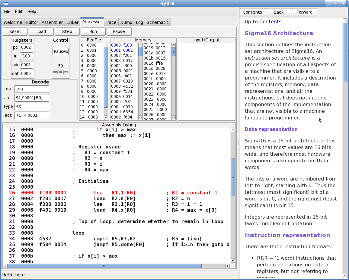
Figure 1: Hydra GUI. The Processor tab is selected, and the machine is running the ArrayMax program.

6.2 Digital circuits

Hydra treats a digital circuit as a function from input signals to output signals. This approach is obvious for combinational circuits, but not for sequential circuits that contain flip flops with state. A key insight is that all circuits, including sequential ones, are pure functions if we model a signal as a stream of values through time, rather than as a value at a point in time.

Since circuits are functions, it becomes easy to specify them in a functional language. Here is the specification of a multiplexer, with control input c and data inputs x and y:

mux1 :: Signal a => a -> a -> a -> a
mux1 c x y = or2 (and2 (inv c) x)
                 (and2 c y)

The type specification (which is optional) says that the circuit has three inputs and one output, and each is a bit signal. The defining equation uses the identifiers c, x, and y as local names for the input signals. It gives the value of the output signal as a function of the inputs.

A register circuit takes a control input ld, and a data input x. It contains an internal state, which is always available on the output. At a clock tick, the register retains its previous state if ld=0, and replaces the state with x if ld=1.

reg1 :: Clocked a => a -> a -> a
reg1 ld x = s
  where s = dff (mux1 ld s x)

The type indicates that reg1 is a synchronous circuit, and its inputs and outputs must have a signal type that knows about clocking.

The examples above show that basic circuits are quite straightforward to specify. These are executable specifications, and by selecting different types to represent the signals, alternative semantics can be selected.

Larger circuits involve large numbers of signals, and it is unwieldy to treat them all as singleton bits. Therefore Hydra allows signals to be grouped together as words and tuples, using the Haskell types for lists and tuples.

Hydra also supports circuits with size parameters, combinators, and generators for specialised kinds of circuit. A circuit generator is a higher order function that generates a circuit, which is itself a first order function. A simple example of a circuit generator is a map function that takes a building block circuit that takes bit inputs and outputs, and replicates the building block to produce a circuit that operates on words rather than bits. A more complex circuit generator takes a control algorithm, expressed as a state machine algorithm, and generates a control circuit.

6.3 Datapath and control

An important concept in designing complex circuits is to partition the design into a datapath and control. The datapath contains the registers and the circuits that perform calculations. The datapath for Sigma16 includes the following equations, which define a set of registers and the output of the ALU:

  (a,b) = regfile n k ctl_rf_ld ir_d rf_sa rf_sb p
  ir = reg n ctl_ir_ld memdat
  pc = reg n ctl_pc_ld r
  adr = reg n ctl_ad_ld q
  (ovfl,r) = alu n ctl_alu_op x y

One of the most interesting aspects of a datapath is that it provides a set of alternative potential operations that can be performed, and these must be supported by multiplexers with corresponding control signals. For example, the first data input to the ALU is called x, and sometimes this should be the value of a (a readout from the register file) and sometimes it should be the pc (in order to increment the pc). To support this, we define x to be the output of a multiplexer that selects between a and pc, and introduce a control signal to determine which value to use. The datapath contains a number of similar equations.

  x  = mux1w ctl_x_pc a pc        -- alu input 1

While the datapath provides potential operations, the control uses a collection of control signals to determine which operations should actually take place during the current clock cycle. There are about 20 control signals in the basic Sigma16 M1 circuit. A few of them are:

  ctl_rf_ld    Load  register file (if 0, remain  unchanged)
  ctl_x_pc     Transmit pc on x (if 0, transmit reg[sa])
  ctl_y_ad     Transmit ad on y (if 0, transmit reg[sb])
  ctl_rf_alu   Input to register file is ALU output (if 0, use m)

6.4 Control algorithm

Textbooks on circuit design often treat control as just another circuit, albeit a large and complex one. There are more sophisticated design methodologies that use Algorithmic State Machines (i.e. flowcharts) to describe the control. One of our conclusions, however, is that it is best to treat control as an algorithm that is expressed in a language, and then to develop systematic methods for synthesising the control circuit.

The control algorithm for Sigma16 is a state machine written in an imperative style. The top of the main loop repeatedly fetches the next instruction and decodes it:

repeat forever
    ir := mem[pc], pc++;
    case ir_op of
      ...

There is a separate case for each instruction; the case for the load instruction (1) fetches the second word of the instruction (the displacement), (2) calculates the effective address, and (3) fetches the data from memory and loads it into the destination register:

  load:
       ad := mem[pc], pc++;
       ad := reg[ir_sa] + ad
       reg[ir_d] := mem[ad]

The control algorithm is a finite state automaton. Alternatively, one can think of the control as a program running on the datapath, which can be thought of as a programming language. This view is natural, because the datapath provides a set of primitive capabilities (e.g. “send the value in the pc to the ALU”, “tell the ALU to increment its input”, and “copy the output from the ALU back to the pc”). By combining and sequencing such primitive operations, the control algorithm causes the datapath to perform useful computations. In order to make the datapath perform the operations specified by the control algorithm, we need to figure out which control signals must be asserted. In general, this can be assisted by software tools, but for a student just learning how a processor works, it’s best to work this out by hand, at least for several instructions.

The following excerpt shows the control algorithm for implementing a load instruction. There are three states, so the algorithm executes in three clock cycles. The first state fetches the address field of the instruction; the second state calculates the effective address; the third state loads the data into the destination register.

  st_load0:
    ad := mem[pc], pc++;
       Assert [ctl_ma_pc, ctl_adr_ld, ctl_x_pc,
               ctl_alu_abcd=1100, ctl_pc_ld]
  st_load1:
    ad := reg[ir_sa] + ad
       Assert [set ctl_y_ad, ctl_alu_abcd=0000,
               set ctl_adr_ld]
  st_load2:
    reg[ir_d] := mem[ad]
       Assert [ctl_rf_ld]

6.5 Running programs on the circuit

The basic circuit (version M1) for the Sigma16 architecture can execute machine language programs, simply by simulating the circuit. However, the circuit contains many input and output signals, and thousands of internal signals. It would be impossible to figure out what is going on by looking at a bit-level simulator.

 

Clock cycle 67
Computer system inputs
         reset=0 dma=0 dma_a=0000 dma_d=0000
ctl_start = 1

Control state
   st_instr_fet = 0  st_dispatch = 0       st_add = 0       st_sub = 0
        st_mul0 = 0     st_cmplt = 0     st_cmpeq = 0     st_cmpgt = 0
       st_trap0 = 0      st_lea0 = 0      st_lea1 = 0     st_load0 = 0
       st_load1 = 0     st_load2 = 0    st_store0 = 0    st_store1 = 0
      st_store2 = 0     st_jump0 = 0     st_jump1 = 0    st_jumpf0 = 0
      st_jumpf1 = 1    st_jumpt0 = 0    st_jumpt1 = 0      st_jal0 = 0
        st_jal1 = 0

Control signals
   ctl_alu_a  = 0 ctl_alu_b  = 0 ctl_alu_c  = 0 ctl_alu_d  = 0
   ctl_rf_ld  = 0 ctl_rf_pc  = 0 ctl_rf_alu = 0 ctl_rf_sd  = 0
   ctl_ir_ld  = 0 ctl_pc_ld  = 1 ctl_ad_ld  = 0 ctl_ad_alu = 0
   ctl_ma_pc  = 0 ctl_x_pc   = 0 ctl_y_ad   = 1 ctl_sto    = 0

Datapath
    ir = f604  pc = 0010  ad = 0011   a = 0000   b = 0012   r = 0011
     x = 0000   y = 0011   p = 0331  ma = 0011  md = 0000 cnd = 0

Memory
   ctl_sto = 0      m_sto = 0
     m_addr = 0011  m_real_addr = 11  m_data = 0000  m_out =0331

Fetched displacement = 0011
jumpf instruction jumped
************************************************************************
Executed instruction:  jumpf  R6,0011[R0]   effective address = 0011
jumped to 0011 in cycle 67
Processor state:    pc = 0010  ir = f604  ad = 0011
************************************************************************

 

Figure 2: Simulation output.

Hydra contains a sublanguage for expressing simulation drivers (also called testbenches). This is a piece of software that accepts input from the user in a readable format, converts it to the bit signal representations, connects the input signals to the circuit, executes the circuit (thereby simulating it), monitors the circuit’s output signals, converts their values to a readable form, and prints that out. Figure 2 shows the output from the simulation driver, as the circuit is on clock cycle 67 while executing the ArrayMax program.

Sometimes it is hard to see what is going on, even looking at the values of registers and signals. Therefore, the simulation driver language maintains a state and provides tools that allow the driver to observe signal values and record partial information as it goes. The simulation driver for Sigma16-M1 watches the output signals from the circuit, collects information, and uses that to print an informative message when a major event (such as the execution of an instruction) occurs. The last few lines of the figure show a message indicating that a jumpf instruction has just executed.

The M1 circuit for Sigma16 takes the simplest approach to solve all the problems needed to execute computer programs. It takes several hours to understand, but average students in the computer architecture course really do understand it. Furthermore, they develop a working understanding, and demonstrate this in exercises that involve modifications (adding new instructions, implementing interrupts, etc.).

There are also circuits that introduce more advanced techniques, including pipelining and superscalar execution. And, with these powerful design techniques, it is quite straightforward to implement different instruction set architectures.

7 Formal methods

Formal methods have been more successful in digital hardware design than in software design. One reason for this is that it’s quick and easy to recompile a program: just type make and wait a minute, but it’s slow and costly to refabricate a circuit: rebuild the masks, send to the foundry, and wait a month. The lazy approach that works for programming fails for hardware design. Another reason is that it is more costly and damaging for a hardware manufacturer to ship chips that don’t work than for a software vendor to ship software that doesn’t work.

The most popular formal method is probably model checking. A pure functional hardware description language also makes it possible to use equational reasoning, which can be used to prove correctness, perform correctness-preserving transformations, and even to derive circuits from specification by calculation.

During the last two years, formal methods have not been used in the fourth-year course on computer architecture, but they were used successfully in the past. (The problem is that there are only 20 lectures available, and far too much material to cover everything.)

A good application of formal methods is in the derivation of a logarithmic time binary addition circuit [8]. This is an excellent example because it yields a very subtle circuit which is quite hard to understand, yet is essential for a fast processor. Indeed, the speedup we obtain by replacing a ripple carry adder by a log time adder is larger than the speedup from larger word sizes, or cache memory, or pipelining, or retiming, or superscalar execution—it is probably the most effective single optimisation available in processor design.

The solution requires first deriving the parallel scan algorithm, followed by a sequence of transformations to a ripple carry adder. Experience shows that a minimum of three lectures are needed for this, and not all students are able to follow the details.

There are many alternative problems that could be used to illustrate formal methods in less time, but they do not make such a convincing case for the power of mathematics.

A limitation of the adder derivation is that this is a combinational circuit. Another direction is to prove correctness of sequential circuits, especially to prove that a circuit correctly implements an instruction set architecture. However, this requires a significant amount of notational machinery (techniques and lemmas) in order to handle the state.

8 Exercises

A central aim of our courses is to help the students to develop a working understanding. Exercises that involve implementation, as well as observing the implementation running in simulation, are a crucial component. Several exercises from recent years are outlined below, including examples from both the required second-year course on computer systems and the elective fourth-year course on computer architecture. The exercises range from quite elementary to fairly advanced. All of these exercises have been solved largely correctly by a majority of students, although there are various glitches and infelicities in many of the solutions.

8.1 Assembly language programming: insertion sort

This exercise is used in the required course on computer systems for second year students.

Problem.

Translate the insertion sort algorithm, which is given as high level pseudocode, into Sigma16 assembly language. Test it on an array of input data using the assembler and emulator. Check that the program is working correctly during execution, and verify that after the program terminates the array is sorted correctly.

Comments.

The lectures emphasise the relationship between high level language constructs (like the statements in the pseudo-code) and instructions. Students are shown how to compile an algorithm to assembly language by hand, and strongly encouraged to do this rather than writing the assembly language code directly. This problem requires ability to handle memory, registers, arrays, index arithmetic, looping, and some simple logical constructs. A systematic commenting style is used consistently in lectures and tutorials, and the students are told that the marking will include assessment of comments. Figure 1 shows a snapshot of the emulator while executing the insertion sort program.

This exercise has been refined over several years, using a number of different algorithms, in order to get a good balance between simplicity and richness of insight. The aim is to give a good understanding of how the instructions work, how they relate to the algorithm, and in general what the machine is doing, but the aim is also to achieve this without needing to write large amounts of boilerplate code.

Many students are completely baffled by this problem when they start. but they receive good support from tutors. The vast majority of students not only succeed in getting this to work, but they also do reasonably well on an unseen assembly language programming problem of similar complexity on the final examination.

8.2 Basic state machines: traffic light controller

Problem.

Design a traffic light controller as a digital circuit. There are two versions. The first version has one input, a pushbutton bit called reset, which is pushed once to start the circuit. There are three output bits corresponding to green, amber, and red, which run through a fixed sequence: green, green, green, amber, red, red, red, red, amber, and so on. The second version models a pedestrian crossing, with a walk request input button; the system controls walk and don’t walk lights as well as the coloured lights for traffic. This version of the circuit should exhibit reasonable behaviour even if the walk request button is pressed frequently. The circuit also maintains a count of walk requests, which could be used by traffic engineers.

Comments.

These circuits are very simple, although they do illustrate some important basic design techniques. The main point of the exercise is to get the students to learn how to write a correct specification in Hydra and run it. It is better to resolve problems with notation on an easy problem like this, than to defer them to a problem where the digital design is challenging.

8.3 ALU

Problem.

Design an arithmetic-logic unit (ALU) that performs integer arithmetic on 8-bit signed integers represented in two’s complement notation. The interface to the circuit is specified with a Hydra (Haskell) type declaration. The circuit inputs are a two-bit opcode op :: (a,a), and two 8-bit words x and y, which are supplied as a group xy :: [(a,a)] in bit slice format. The outputs are (ofl, r) :: (a, [a]), where ofl indicates overflow, and r is the 8-bit result word. The value of the output r depends on the value of the control input op, as follows:

op	$r$
(0,0)	$x+y$
(0,1)	$x-y$
(1,0)	$y+1$
(1,1)	$-y$

Comments.

This is a combinational design, with no circuit state such as flip flops. Several interesting techniques need to be combined to solve the problem. The best approach is to use a single binary word adder, and to make the adder perform all the required operations by preprocessing the inputs and postprocessing the outputs. The mscanr higher order function gives a simple, elegant, and general definition of the adder. The bit slice organisation is useful for incorporating the ALU into larger circuits, and also provides useful experience with types and patterns.

8.4 Pipelined integer vector multiplier

Problem.

Design a circuit that inputs a pair of $k$-bit binary integers on every clock cycle. After $k$ cycles, the circuit outputs the $2\times k$-bit result. The circuit needs to be pipelined, as a new pair of integers are read in every cycle.

Comments.

The students have already been shown a sequential multiplier functional unit based on the “shift and add” algorithm. The essence of the problem is to transform a sequential circuit that uses registers for in-place state into a pipelined circuit that unfolds the iteration into a sequence of states.

8.5 Loadxi instruction

Problem.

Add a new instruction to the Sigma16 architecture, as defined below. Modify the datapath and control, as needed, in order to implement the new instruction in the M1 circuit. Modify the test bench so the operation of the instruction can be observed, and demonstrate the execution of the instruction using a machine language test program.

The new instruction is load with automatic index increment (the loadxi instruction). Its format is RX: there are two words; the first word has a 4-bit opcode f, a 4-bit destination register (the d field), a 4-bit index register (the sa field), and a 4-bit RX opcode of 7 (the sb field). As with all RX instructions, the second word is a 16-bit constant called the displacement. In assembly language the instruction is written, for example, as loadxi R1,$12ab[R2].

The effect of executing the instruction is to perform a load, and also to increment the index register automatically. The effective address is calculated using the old value of R2 (i.e. the value before it was incremented.) Thus the instruction loadxi R1,$12ab[R2] performs R1 := mem[12ab+R2], R2 := R2+1.

Comments.

This exercise requires changes to about a dozen lines of code (including comments). However, it is necessary to understand how the datapath, control algorithm, and control circuit work in order to make those changes. The assignment handout asks for a status report that includes an explanation of how the instruction was implemented, as well as a machine language program that demonstrates the instruction and simulation output showing that the instruction works correctly. A large majority of the students succeeded, while some others outlined what needs to be done but didn’t complete the modifications.

8.6 The multiply instruction

Problem.

The version of Sigma16 that is provided to the students has a Multiply instruction, but it acts as a “nop”: it does nothing at all. The students have also been given a standalone multiplier functional unit circuit, as a simple example of sequential design. The problem is to make the multiply instruction work correctly, and to demonstrate its operation by simulating the processor as it executes a suitable test program.

Comment.

This problem is about processor design, not about multiplication, since the multiplier circuit has been provided. The main complication is that the multiplier circuit takes a variable amount of time, depending on the values of the inputs, and the processor control needs to take account of this. Changes are required to the datapath, control algorithm, and control circuit. In addition, changes should be made to the testbench definition, so the operation of the multiplier can be observed as the circuit operates.

9 Experience and observations

The observations in this section are based on the author’s own experiences. It would be interesting to compare them with the experiences of other lecturers at other universities in other countries.

For the most part, students have reacted enthusiastically to the approach presented here. Many of them find it enlightening and fun to see a digital circuit running computer programs, and they feel they really understand what is happening when they modify the circuit to add a new instruction. Nearly all the students who put in a reasonable effort are able to learn the language, understand the circuit examples, and carry out the exercises successfully.

9.1 Systems issues

Connecting the dots.

The deepest benefits from learning about circuits and computer architecture come from connecting the concepts, not just learning them in isolation. This means, for example, using the material on digital circuits to implement an instruction set architecture, and using the material on instruction sets to implement core operating system facilities. These connections are more valuable than the specific details at any one level of abstraction.

Executing circuits and programs.

A great benefit from using a hardware description language is that students can watch circuits operate by simulating them, and can execute programs by emulating them or running them on a simulated circuit. Simulation helps to get a working understanding of what a computer is doing, and this understanding is far deeper than what can be attained by a vague descriptive approach.

Choice of topics.

Computer systems contain many levels of abstraction, and there is an enormous amount of interesting material at each one of them. A tiny subset of the material at each level must be selected. Many textbooks spend too much time covering lots of ancillary details, preventing them from getting to the most interesting topics (the ones that are needed to connect the dots). For example, it is common for textbooks on digital design to present a wide range of SSI and MSI components, and a variety of different kinds of flip flop, yet most of those components became obsolete decades before our students were born. It is much better to skip most of the components, and most of the optimisation techniques, and go straight to the essential components and methods needed to see how realistic circuits work, and to develop those circuits toward a processor.

The choice of topic depends heavily on the time available. Within 20 lectures, it is quite realistic to explain digital components, circuits, and move up to a complete processor circuit, all within 12 lectures, leaving time for advanced topics like pipelining and superscalar, to fit within a 20 lecture course. We have an existence proof that this is possible! But such an ambitious goal requires ruthless care in selection of topics. If more time is available, there is naturally a wealth of additional material to enrich the course.

Simulation or real hardware?

An endless debate in computer systems education is whether to have students run exercises on real hardware, or on simulated (or emulated) hardware. This debate arises at all levels, including circuit design and machine language programming. There are many advantages of simulation and emulation:

• A better environment for tracing and debugging is available.

• A variety of alternatives (e.g. variations on instruction set architectures) can be provided, with little overhead.

• The particular systems studied (machine languages, digital circuits) can be designed specifically for the intended purpose, and are not encumbered with all the irrelevant complexity that comes with “real” systems.

• Aspects of the system that are not central can be glossed over, while they may require great complexity on real hardware. For example, you can’t run a program on a digital circuit without getting the initialisation right, and the initialisation can easily be more complicated than all the rest of the system. With a simulator, the initialisation can be performed deus ex machina.

• Glossing over the minor details leaves more time for the essential ideas. Indeed, it is unusual to have a course that starts with circuit design and attains a complete processor circuit within 12 lectures, and that would be impossible using real hardware.

The advantages claimed for using real hardware are unconvincing:

• “It motivates students to learn about real products, rather than systems that abstract away irrelevant details.” This claim sounds hollow when students are faced with the details of incrementing the pc register on a Pentium, or bootstrapping a loader.

• “Students appreciate the levels of abstraction in computer systems better when they know that they are seeing real software running on real hardware.” This claim is extremely naive. If a student writes an x86 program and runs it on a Pentium chip, is their software running on real hardware or via layers of firmware and emulation? The answer depends on which model of chip is in their computer!

Granularity of the time scale.

The events that occur in a digital circuit take place on a short time scale, with massive parallelism. The events that occur at the instruction set level exhibit far less parallelism, and the time scale is two to three orders of magnitude longer. These differences in scale are interesting, and they do not cause problems with simulation. For example, experience shows that students can follow all the details, and fully understand, the processor circuit as it runs a real machine language program. However, as we move up to the level of operating systems, the varying time scales pose real difficulties. To study the operation of virtual memory in detail, we have to consider some events that occur in a fraction of a clock cycle, and other events that occur on the time scale of disk access. These time scales differ by nine orders of magnitude. It is challenging even to get across to some students what the term “nine orders of magnitude” means. However, these topics can be addressed in detail by combining detailed circuit simulation where appropriate (e.g. the TLB) with coarser grained emulation; the problem is that connecting the dots between these levels must be done semiformally, with some verbal explanation.

Models.

A language isn’t enough: it is important to describe clearly the circuit models that are being used. A model is an abstraction that ignores some aspects of the hardware’s behaviour, providing a view that is simple enough to work with effectively. The work described in this paper is based on a pure synchronous model with a single-phase clock. Some other circuit models can be handled by Hydra, but not all. It is a fallacy to say that we don’t need models, because we will look at how the hardware “really” works. “Real” digital hardware actually consists of analogue circuits that are carefully designed and operated so as to exhibit mostly digital behaviour most of the time. The details of this are extraordinarily complicated [10], and should not be discussed until and unless students have fully mastered the synchronous model.

Karnaugh maps.

Some students have an obsession with Karnaugh maps, which are covered in the short section of the first year course on computer hardware. A Karnaugh map is an optimisation technique, not a design technique, yet some students claim not to know how to design a simple combinational circuit without starting with a Karnaugh map. There are two problems with this: (1) a basic principle in computer science is to start with the specification, then perform optimisation as needed; and (2) Karnaugh maps make a circuit more efficient according to the component-count metric, but they may make a circuit less efficient according to other cost models—especially the area-based cost models that are relevant to VLSI design. At best, a Karnaugh map is a small scale transformation, akin to rearranging a few instructions to save an instruction or two, but they do not address the larger scale algorithmic issues that dominate circuit performance.

9.2 Language issues

Benefits of a functional hardware description language.

The observed benefits include a good match between the foundation of the language (functions) and the foundations of circuits (functions); a precise language that allows clearer specifications than are possible with vague diagrams; ability to define sublanguages for clear description of specialised circuits such as control algorithms; improved abstraction using design patterns expressed as higher order functions; executable specifications; typechecking circuit interfaces; and effective formal methods with equational reasoning.

Language preferences.

A number of students in the fourth-year course are extremely enthusiastic about the functional hardware description language, and are keen to use it further in projects, internships, or research projects. Feedback from these students indicates that they like the power and simplicity of the specification, especially the ability to design a digital circuit from the ground up that can actually run computer programs—”connecting the dots”. On the other hand, some students in the fourth-year course say that VHDL should be used because that is an industry standard language. The students who have given this feedback are doing a combined degree with electrical engineering.

Prerequisites.

No matter what language is used for describing hardware, there will be some students who don’t know it. To make the course materials described in this paper more widely useful, an aim is to make the course self-contained, so that knowledge of functional programming in general or Haskell in particular is not a prerequisite. This is achieved by (1) not using the full Haskell language, but rather a much smaller Hydra language; (2) teaching Hydra from the ground up, which takes little time because the language is so small; (3) implementing Hydra with a transformation tool that provides an error message if the user steps outside Hydra into Haskell.

Syntax.

The semantics of a language is more fundamental than its surface syntax, but some feel uncomfortable if the syntax looks superficially unfamiliar. The layout rule, in particular, seems to help stronger students (the code is more concise and readable) but to confuse weaker ones (who often avoid indentation entirely, and just write each line of code beginning in the leftmost character position).

Picky details.

There are a lot of little details in digital circuits that can be glossed over when giving a vague description, but that have to be handled precisely correctly in order to get a correct specification that can be simulated and executed successfully. One example of this is in bundling a group of signals into a cluster, such as a word or tuple of signals. Many publications on circuits, including research papers as well as textbooks, use informal notations for clusters of signals that give a general idea of what is going on, but that rely on a full understanding in order to get the circuit actually to work. Hydra contains several kinds of machinery, largely inherited from the Haskell type system, to help with these details. Nevertheless, it takes some time to cover the necessary language features, and students often get type errors when they mix up the signal clusters. (These issues also arise in standard languages like VHDL and informal notations such as used in the Hennessey and Patterson books—if you want a precise specification, you have to get the picky details right, and the expressive type system of the functional language helps significantly.)

Hardware or software?

Any hardware description language will look like software to weaker students, who will not understand the distinction between the circuit and the software notations used to specify the circuit. This happens because of inadequate thinking about abstraction, not as a result of the choice of a functional or imperative hardware description language.

DSL error messages.

Hydra is a domain specific language (DSL) implemented by embedding in Haskell. The benefits of this approach have been discussed extensively in the literature. A drawback—which has also been widely recognised—is that error messages often come from the host language rather than from the DSL, so they make little sense to the end user. Thus it is possible to make an error in a circuit specification, and to receive an error message that relates to Haskell rather than to the circuit. The new transformation system for Hydra is currently being developed, and this appears to help greatly by having an explicit representation of the Hydra language per se, but further experimentation will be needed to evaluate this.

9.3 Educational issues

Expectations.

It would be wonderful if the use of some secret magic bullet would cause all students to master the computer systems material, and go on to become real experts. Alas, this just doesn’t happen—not even when functional programming is used. The author’s personal experience is that the weakest students learn little, regardless of what techniques are used. However, the strongest students learn much more using the functional hardware description language: they really do achieve the working understanding which is the aim.

Exercises.

The exercises, where students design circuits and observe their execution, are vital to mastering the material. It is tempting to make all the exercises interesting and challenging, but that is a mistake: It is essential to begin with some very straightforward exercises to gain familiarity with the software tools. It isn’t enough to give lots of examples, and then to assign an exercise that assumes the students have assimilated the elementary aspects of the examples.

10 Conclusion

It is better to use a hardware description language than just showing some schematic diagrams when teaching circuit design, especially for large and complex circuits. A functional hardware description language offers numerous additional benefits over an imperative one: more concise specifications of circuits, a clear connection to the view of circuits as functions, alternative circuit semantics, and clean integration with formal methods. Using this approach, it is possible to show a complete digital circuit that fully implements a processor, with the ability to run programs by simulating the circuit, and this greatly motivates the stronger students.

References

- [1]
- [2] Per Bjesse, Koen Claessen & Mary Sheeran (1998): Lava: Hardware Design in Haskell. In: Proceedings of the third ACM SIGPLAN International Conference on Functional Programming, ACM, pp. 174–184, 10.1145/289423.289440.
- [3] David Money Harris & Sarah L. Harris (2013): Digital Design and Computer Architecture, second edition. Elsevier, 10.1016/B978-0-12-394424-5.00004-5. ISBN 978-0-12-394424-5.
- [4] Steven D. Johnson (1984): Applicative Programming and Digital Design. In: 11th Annual ACM Symposium on Principles of Programming Languages, ACM, pp. 218–227, 10.1145/800017.800533.
- [5] Noam Nisan & Shimon Schocken (2005): The Elements of Computing Systems: Building a Modern Computer from First Principles. The MIT Press. ISBN 0-262-14087-X.
- [6] John O’Donnell (1995): From transistors to computer architecture: Teaching functional circuit specification in Hydra. In: FPLE’95: Symposium on Functional Programming Languages in Education, LNCS 1022, Springer-Verlag, pp. 195–214, 10.1007/3-540-60675-0_46.
- [7] John O’Donnell (2002): Overview of Hydra: A Concurrent Language for Synchronous Digital Circuit Design. In: Proceedings 16th International Parallel & Distributed Processing Symposium, IEEE Computer Society, p. 234 (abstract), 10.1109/IPDPS.2002.1016653. Workshop on Parallel and Distribued Scientific and Engineering Computing with Applications—PDSECA.
- [8] John O’Donnell & Gudula Rünger (2004): Derivation of a Logarithmic Time Carry Lookahead Addition Circuit. Journal of Functional Programming 14(6), pp. 697–713, 10.1017/S0956796804005180.
- [9] David A. Patterson & John L. Hennessy (1998): Computer Organization & Design: The Hardware/Software Interface, second edition. Morgan Kaufmann.
- [10] John F. Wakerly (2000): Digital Design: Principles & Practices, third edition. Prentice Hall International.
- [11] David E. Winkel & Franklin P. Prosser (1986): The Art of Digital Design: An Introduction to Top-down Design, second edition. Prentice-Hall.