Improved Approximation Algorithms for Computing $k$ Disjoint Paths Subject to Two Constraints

Abstract

For a given graph $G$ with positive integral cost and delay on edges, distinct vertices $s$ and $t$, cost bound $C\in Z^{+}$ and delay bound $D\in Z^{+}$, the $k$ bi-constraint path ($k$BCP) problem is to compute $k$ disjoint $st$-paths subject to $C$ and $D$. This problem is known NP-hard, even when $k=1$ [4]. This paper first gives a simple approximation algorithm with factor-$(2,2)$, i.e. the algorithm computes a solution with delay and cost bounded by $2*D$ and $2*C$ respectively. Later, a novel improved approximation algorithm with ratio $(1+\beta,\,\max\{2,\,1+\ln\frac{1}{\beta}\})$ is developed by constructing interesting auxiliary graphs and employing the cycle cancellation method. As a consequence, we can obtain a factor-$(1.369,\,2)$ approximation algorithm by setting $1+\ln\frac{1}{\beta}=2$ and a factor-$(1.567,\,1.567)$ algorithm by setting $1+\beta=1+\ln\frac{1}{\beta}$. Besides, by setting $\beta=0$, an approximation algorithm with ratio $(1,\,O(\ln n))$, i.e. an algorithm with only a single factor ratio $O(\ln n)$ on cost, can be immediately obtained. To the best of our knowledge, this is the first non-trivial approximation algorithm for the $k$BCP problem that strictly obeys the delay constraint.

k$-disjointbi-constraintpath,NP-hard,bifactorapproximationalgorithm,auxiliarygraph,cyclecancellation.\par$

1 Introduction

In real networks, there are many applications that require quality of service and some degree of robustness simultaneously. Typically, the quality of service (QoS) related problem requires routing between the source node and the destination node to satisfy several constraints simultaneously, such as bandwidth, delay, cost and energy consumption. Nevertheless, in networks, some time-critical applications also require routing to remain functioning while edge or vertex failure occurs. A common solution is to compute $k$ disjoint paths that satisfy the QoS constraints, and use one path as an active path whilst the other paths as backup paths. The routing traffic is carried on the active path, and switched to the disjoint backup paths while an edge or vertex failure occurs on the active path. However, for some time-critical applications even the time to discover failures of routing and restore data transmission in backup paths is too long for them. For such applications, packages are routed via $k$ paths simultaneously, and the traffic is switched from failed paths to functioning paths if edge or vertex failures occur, such that routing can tolerate $k-1$ edge (vertex) failures. Therefore, given cost and delay as the QoS constraints, the disjoint QoS Path problem arises as below:

Definition 1

For a graph $G=(V,\,E)$ and a pair of distinct vertices $s,\,t\in V$, a cost function $c:E\rightarrow Z^{+}$, a delay function $d:E\rightarrow Z^{+}$, a cost bound $C\in Z^{+}$ and a delay bound $D\in Z^{+}$, the $k$-disjoint QoS Paths problem is to compute $k$ disjoint $st$-paths $P_{1},\dots,P_{k}$, such that $\underset{i=1,\dots,k}{\sum}c(P_{i})\leq C$ and $d(P_{i})\leq D$ for every $i=1,\dots,k$.

This problem is NP-hard even when all edges of $G$ are with cost 0 [8], which results in the difficulty to approximate the $k$-disjoint QoS Paths problem. An alternative method is to compute $k$ disjoint with total cost bounded by $C$ and delay bounded by $D$ ( equal to $kD$ in Definition 1), and then route the packages via the paths according to their urgency priority, i.e., route urgent packages via paths of low delay whilst deferrable ones via paths of high delay of the $k$ disjoint paths. Therefore, The disjoint bi-constraint path problem arises as in the following:

Definition 2

(The $k$ disjoint bi-constraint path problem, $k$BCP) For a graph $G=(V,E)$ with a pair of distinct vertices $s,t\in V$, a cost function $c:E\rightarrow R^{+}$, a delay function $d:E\rightarrow R^{+}$, a cost bound $C\in Z^{+}$ and a delay bound $D\in R^{+}$, the $k$-disjoint bi-constraint path problem is to calculate $k$ disjoint $st$-paths $P_{1},\dots,P_{k}$, such that $\underset{i=1,\dots,k}{\sum}c(P_{i})\leq C$ and $\underset{i=1,\dots,k}{\sum}d(P_{i})\leq D$.

This paper will focus on bifactor approximation algorithms for the $k$BCP problem, which are introduced as below:

Definition 3

An algorithm $A$ is a bifactor $\left(\alpha,\,\beta\right)$-approximation for the $k$BCP problem, if and only if for every instance of $k$BCP, $A$ computes $k$ disjoint $st$-paths of which the delay sum and the cost sum are bounded by $\alpha*D$ and $\beta*C$ respectively.

Since a $\beta$-approximation with the single factor ratio on cost is identical to a bifactor $\left(1,\,\beta\right)$-approximation, we use them interchangeably in the text.

1.1 Related work

This $k$BCP problem is NP-hard even when $k=1$ [4]. To the best of our knowledge, this paper is the first one that presents non-trivial approximation algorithms for the $k$BCP problem formally. However, a number of papers have addressed problems closely related to $k$BCP, in particular the $k$ restricted shortest path problem ($k$RSP), which is to calculate $k$ disjoint $st$-paths of minimum cost-sum under the delay constraint $\underset{i=1,\dots,k}{\sum}d(P_{i})\leq D$. An algorithm with bifactor approximation ratio $(2,\,2)$ has been developed in [6] for general $k$, while no approximation solution that strictly obeys the delay (or cost) constraint is known even when $k=2$. For a positive real number $r$, bifactor ratio of $(1+\frac{1}{r},\,r(1+\frac{2(\log r+1)}{r})(1+\epsilon))$ and $(1+\frac{1}{r},\,r(1+\frac{2(\log r+1)}{r}))$ have been achieved respectively in [10, 3] for the case $k=2$ and under the assumption that the delay of each path in the optimal solution of $k$RSP is bounded by $\frac{D}{k}$.

Special cases of this problem have been studied. When the delay constraint is removed, this problem is reduced to the min-sum problem, which is to calculate $k$ disjoint paths with the total cost minimized. This problem is known polynomially solvable [11]. Moreover, when $k=1$, the problem reduces to the single bi-constraint path (BCP) problem, which is known as the basic QoS routing problem [4] and admits full polynomial time approximation scheme (FPTAS) [4, 9]. Recently, the single BCP problem is still attracting considerable interests of the researchers. The strongest result known is a ($1+\epsilon$)-approximation due to Xue et al [14].

Additionally, when the cost constraint is removed, the disjoint QoS problem reduces to the length bounded disjoint path problem of finding two disjoint paths with the length of each path constrained by a given bound. This problem is a variant of the min-Max problem of finding two disjoint paths with the length of the longer path minimized . Both of the two problems are known to be NP-complete [8], and with the best possible approximation ratio of 2 in digraphs [8], which can be achieved by applying the algorithm for the min-sum problem in [11, 12]. Contrastingly, the min-min problem of finding two paths with the length of the shorter path minimized is NP-complete and doesn’t admit $K$ approximation for any $K\geq 1$ [5, 13, 2]. The problem remains NP-complete and admits no polynomial time approximation scheme in planar digraphs [7].

1.2 Our techniques and results

The main result of this paper is a factor-$(1+\beta,\,\max\{2,\,1+\ln\frac{1}{\beta}\})$ approximation algorithm for any $0<\beta\leq 1$ for the $k$BCP problem. The main idea of the algorithm is firstly to compute $k$-disjoint paths with delay-sum bounded by $\alpha D$ and cost-sum bounded by $(2-\alpha)*C$, where $0\leq\alpha\leq 2$ is a real number, and secondly to improve the computed $k$ paths by novelly combining cycle cancellation [10] and cost-bounded auxiliary graph construction [14]. The key technique to prove the algorithm’s approximation ratio is using definite integral to compute a close form for the sum of the cost increment during the improving phase.

As a consequence of the main result, we can obtain a factor-$(1.369,\,2)$ approximation algorithm by setting $1+\ln\frac{1}{\beta}=2$, and a factor-$(1.567,\,1.567)$ algorithm by setting $1+\beta=1+\ln\frac{1}{\beta}$ and slightly modifying our algorithm (to improve either cost or delay that is with worse ratio). Nevertheless, by slightly modifying our ratio proof, we show that an approximation algorithm with ratio $(1,\,O(\ln n))$, i.e. an algorithm with single factor ratio of $O(\ln n)$ on cost, can be immediately obtained by setting $\beta=0$. To the best of our knowledge, this is the first non-trivial approximation algorithm for the $k$BCP problem that strictly obeys the delay constraint.

We note that our algorithms are with pseudo-polynomial time complexity, since the auxiliary graph we construct is of size $O(C*n)$. However, by using the classic polynomial time approximation scheme design technique [4], i.e. for any small $\epsilon>0$ setting the cost of every edge to $\left\lfloor\frac{c(e)}{\frac{\epsilon C}{n}}\right\rfloor$ in $G$ before the construction of auxiliary graph, we can immediately obtain a polynomial time algorithm with ratio $((1+\beta)*(1+\epsilon),\,\max\{2,\,1+\ln\frac{1}{\beta}\}*(1+\epsilon))$. We shall omit the details due to the paper length limitation.

2 An improved approximation algorithm for computing $k$ disjoint bi-constraint paths

This section will first present a simple approximation method for computing $k$-disjoint paths with delay-sum bounded by $\alpha D$ and cost-sum bounded by $(2-\alpha)*C$, where $0\leq\alpha\leq 2$ is a real number, and secondly improve the computed $k$ paths by balancing the value of $\alpha$ and $2-\alpha$. Though the presented simple algorithm is with worse ratio than that of the algorithm for $k=2$ in [10], it suits the improving phase better.

2.1 A basic approximation algorithm

Observing that the difficulty of computing $k$-disjoint bi-constraint paths mainly comes from the two given constraints, the key idea of our algorithm is to deal with one new constraint $B$ instead of the two given constraints $C$ and $D$. Our algorithm firstly assigns a new mixed cost $b(e)=\frac{c(e)}{C}+\frac{d(e)}{D}$ to every edge in graph, and secondly computes $k$ disjoint paths with the new cost sum bounded by $B=\frac{C}{C}+\frac{D}{D}=2$. Note that the second step can be accomplished in polynomial time by employing the SPP algorithm due to Suurballe and Tarjan [11, 12]. The detailed algorithm is as in Algorithm 1.

Input: A graph $G=(V,E)$, each edge $e$ with cost $c(e)$ and delay $d(e)$, a given cost constraint $C\in Z^{+}$ and delay constraint $D\in Z^{+}$;

Output: $k$ disjoint paths $P_{1},\,P_{2}\,\dots,P_{k}$.

1. Set the new cost of edge $e$ as $b(e)=\frac{c(e)}{C}+\frac{d(e)}{D}$;

2. Compute the $k$ disjoint paths $P_{1},\,P_{2}\,\dots,P_{k}$ in $G$ by using Suurballe and Tarjan’s algorithm [11, 12], such that $\sum_{i=1}^{k}\sum_{e\in P_{i}}b(e)$ is minimized;

3. Return $P_{1},\,P_{2}\,\dots,P_{k}$.

Algorithm 1 A basic approximation algorithm for the $k$-BCP problem

The time complexity and performance guarantee of Algorithm 1 is given by the following theorem:

Theorem 4

Algorithm 1 runs in $O(km\log_{1+\frac{m}{n}}n)$ time, and computes $k$-disjoint paths with delay-sum bounded by $\alpha D$ and cost-sum bounded by $(2-\alpha)*C$ , where $0\leq\alpha\leq 2$ is a real number.

Proof

The main part of Algorithm 1 takes $O(km\log_{1+\frac{m}{n}}n)$ to compute $k$-disjoint paths by using Surrballe and Tarjan’s algorithm [11, 12], and other parts of the algorithm take trivial time. Hence the time complexity of the algorithm is $O(km\log_{1+\frac{m}{n}}n)$.

It remains to show the approximation ratio. To make the proof concise, we denote by $OPT$ an optimal solution for the $k$-disjoint BCP paths problem, and $SOL$ the solution of Algorithm 1. Obviously $\sum_{e\in OPT}b(e)\leq 2$ holds. Then since the $k$ disjoint paths is with minimum new cost, we have

$$\sum_{e\in SOL}b(e)\leq\sum_{e\in OPT}b(e)\leq 2.$$ (1)

Assume the delay-sum of the algorithm is $\alpha$ times of $d(OPT)$, then following Algorithm 1 $0\leq\alpha\leq 2$ holds. Therefore, we have $\sum_{e\in SOL}b(e)=\sum_{i=1}^{k}\sum_{e\in P_{i}}b(e)=\alpha+\frac{c(SOL)}{c(OPT)}$. From Inequality (1), $\alpha+\frac{c(SOL)}{c(OPT)}\leq 2$ holds. That is, $c(SOL)\leq(2-\alpha)c(OPT)\leq(2-\alpha)C$. This completes the proof.

Note that $\alpha$ differs for different instances, i.e. Algorithm 1 may return a solution with cost $2*c(OPT)$ and delay $0$ for some instances, while a solution with cost 0 and delay $2*d(OPT)$ for other instances. Hence, the bifactor approximation ratio for Algorithm 1 is actually $(2,2)$.

In real networks, the two given constraints may not be of equal importance, say, delay is far more important comparing to cost. In this case, applications require that the delay of the resulting solution is bounded by $(1+\beta)D$, where $0<\beta<1$ is a positive real number. Apparently, we could get an algorithm similar to Algorithm 1 excepting setting the new cost as $b(e)=\beta\frac{c(e)}{C}+\frac{d(e)}{D}$. The ratio of the new algorithm is given as below:

Corollary 5

By setting the new cost as $b(e)=\beta\frac{c(e)}{C}+\frac{d(e)}{D}$ for a given real number $0<\beta<1$ , Algorithm 1 returns $k$ paths with delay-sum bounded by $\alpha D$ and cost-sum bounded by $\frac{1+\beta-\alpha}{\beta}*C$ , where $0\leq\alpha\leq 1+\beta$ is a real number. Therefore the ratio of the algorithm is $(1+\beta,\,1+\frac{1}{\beta})$.

The proof of Corollary 5 is omitted here, since it is very similar to the proof of Theorem 1. According to Corollary 5, our algorithm can bound the delay-sum of the $k$-disjoint path by $(1+\beta)D$ for any $0<\beta<1$, by relaxing the cost constraint to $(1+\frac{1}{\beta})*C$. For example, if $\beta=0.01$, then the bifactor approximation ratio of the algorithm is $(1.01,\,101)$. Thus, the algorithm decrease the delay of the $k$-disjoint paths at a high price. In the next subsection, we shall develop an improved method that pays less to make delay-sum of the $k$-disjoint paths bounded by $(1+\beta)D$.

2.2 The improving phase

To make the delay of the solution resulting from Algorithm 1 bounded by $(1+\beta)$D, our improving phase is, basically a greedy method, using the so-called cycle cancellation to improve the disjoint paths in iterations until a solution with the best possible ratio $(1+\beta,\,\max\{2,1+\ln\frac{1}{\beta}\})$ is obtained. The cycle cancellation method is an approach of using cycles to change the edges of the disjoint paths, which first appears in [10] and is derived from the following proposition that can be immediately obtained from flow theory [1]:

Proposition 6

Let $P_{1},\,P_{2}\,\dots,\,P_{k}$ and $Q_{1},\,Q_{2}\,\dots,Q_{k}$ be two sets of $k$ disjoint $st$-paths in $G$, $\overline{G}$ be $G$ excepting that all edges of $P_{1},\,P_{2}\,\dots,P_{k}$ are reversed, and $O$ be a cycle in $\overline{G}$. Then

1. The edges of $P_{1},\,P_{2}\,\dots,\,P_{k}$ and $O$, excepting the pairs of parallel edges with opposite direction, compose $k$-disjoint paths;

2. There exist a set of edge disjoint cycles $O_{1},\,\dots,\,O_{h}$ in $\overline{G}$, such that the edges of $P_{1},\,P_{2}\,\dots,\,P_{k}$ and $O_{1},\,\dots,\,O_{h}$, excepting the pairs of parallel edges with opposite direction, compose $Q_{1},\,Q_{2}\,\dots,Q_{k}$.

From the proposition above, it is obvious that there exists a set of cycles $O_{1},\,\dots,\,O_{h}$ that can improve $k$ disjoint QoS paths $P_{1},\,P_{2}\,\dots,P_{k}$ to an optimal solution. However, it is hard to identify all the cycles $O_{1},\,\dots,\,O_{h}$, so we employ a greedy approach to compute a set of cycles to obtain an approximation approach. The improving phase is composed by iterations, each of which computes a cycle and then uses it to improve $P_{1},\,P_{2}\,\dots,\,P_{k}$. More precisely, to obtain a good ratio, the algorithm computes in iteration $j$ a cycle $O_{j}$ with $\frac{d(O_{j})}{c(O_{j})}$ minimized among the cycles in $\overline{G}$. The layout of the algorithm is as given in Algorithm 2.

Input: A graph $G=(V,E)$, each edge $e$ with cost $c(e)$ and delay $d(e)$, a given cost constraint $C\in Z^{+}$ and delay constraint $D\in Z^{+}$, disjoint QoS paths $P_{1},\,P_{2}\,\dots,P_{k}$ computed by Algorithm 1;

Output: Improved disjoint QoS paths $Q_{1},\,Q_{2}\,\dots,Q_{k}$.

1. If $\sum_{i=1}^{k}d(P_{i})\leq(1+\beta)D$ ;

   then return $P_{1},\,P_{2}\,\dots,P_{k}$ as $Q_{1},\,Q_{2}\,\dots,Q_{k}$ , terminate;

2. Reverse direction of the edges of $P_{1},\,P_{2}\,\dots,P_{k}$ in $G$ , set their cost to a small positive real number $0<\epsilon<\frac{1}{mnD}$, and negative their delay;

3. Compute cycle $O_{j}$ with $c(O_{j})\leq C$, $d(O_{j})<0$ and $\frac{d(O_{j})}{c(O_{j})}$ attaining minimum, by the method given in next section;

   /* Following clause 2 of Proposition 6, if $\sum_{i=1}^{k}d(P_{i})\geq d(OPT)$ and $\sum_{i=1}^{k}c(P_{i})\geq 0$, there always exist cycle $O_{j}$ with $c(O_{j})\leq C$ and $d(O_{j})<0$. */

4. Improve $P_{1},\,P_{2}\,\dots,P_{k}$ by adding the edges of $O_{j}$ and removing the pairs of parallel edges in opposite direction;

5. Go to Step 1.

Algorithm 2 An improved algorithm based on cycle cancellation.

Following clause 1 of Proposition 6, Algorithm 2 will correctly return $k$ disjoint paths. It remains to show the cost and delay of the $k$ disjoint paths is constrained as below:

Theorem 7

The approximation ratio of Algorithm 2 is $(1+\beta,\>\max\{2,\,1+\ln\frac{1}{\beta}\})$.

Proof

For the case that $\sum_{i=1}^{k}d(P_{i})\leq(1+\beta)D$ holds before the improving phase, the approximation ratio of Algorithm 2 is obviously $(1+\beta,\,2)$.

It remains to show the ratio of the algorithm is $(1+\beta,\>1+\ln\frac{1}{\beta})$ for the case that $\sum_{i=1}^{k}d(P_{i})>(1+\beta)D$. Assume that Algorithm 2 runs in $h$ iterations, the key idea of the proof is to sum up the cost increment while using the cycle to improve the $k$ disjoint paths in iterations, and show that the cost sum is bounded (by giving the cost sum a close form).

Note that in the case, we have $\alpha D\geq\sum_{i=1}^{k}d(P_{i})>(1+\beta)D$, so $\alpha>1+\beta$ holds. Let $\Delta D=d(OPT)-d(SOL)\geq(1-\alpha)d(OPT)$ and $\Delta C=c(OPT)-c(SOL)\leq(\alpha-1)c(OPT)$. Clearly, $\Delta D<0$ and $\Delta C>0$ hold. Let the cycle computed in the $j$th iteration be $O_{j}$, then since $\frac{d(O_{j})}{c(O_{j})}$ attains minimum in Step 3 of Algorithm 2, we have $\frac{d(O_{j})}{c(O_{j})}\leq\frac{\Delta D-\sum_{i=1}^{j-1}d(O_{i})}{C}.$ That is,

$$c(O_{j})\leq\frac{d(O_{j})}{\Delta D-\sum_{i=1}^{j-1}d(O_{i})}C.$$

By summing up $c(O_{j})$ in $h-1$ iterations (excluding the last iteration), we have:

$$\sum_{j=1}^{h-1}c(O_{j})\leq C\sum_{j=1}^{h-1}\frac{d(O_{j})}{\Delta D-\sum_{i=1}^{j-1}d(O_{i})}.$$

Following the definition of Definite Integral, we have:

$$\sum_{j=1}^{h-1}\frac{d(O_{j})}{\Delta D-\sum_{i=1}^{j-1}d(O_{i})}=\sum_{j=1}^{h-1}\frac{1}{\Delta D-\sum_{i=1}^{j-1}d(O_{i})}d(O_{j})\leq\int_{\Delta D}^{\Delta D-\sum_{i=1}^{h-1}d(O_{i})}\frac{1}{x}dx,$$ (2)

where the maximum is attained when $d(O_{j})=-1$ for every $j$.

Algorithm 2 terminates when $d(SOL)+\sum_{i=1}^{h}d(O_{i})\leq(1+\beta)D$, so in the $h-1$ iterations $d(SOL)+\sum_{i=1}^{h-1}d(O_{i})>(1+\beta)D$ holds. That is $d(SOL)-D+\sum_{i=1}^{h-1}d(O_{i})>\beta D$, and hence $-\Delta D+\sum_{i=1}^{h-1}d(O_{i})>\beta D>0$ holds. So we obtain a close form for the cost sum of the $h-1$ iterations:

$$\int_{\Delta D}^{\Delta D-\sum_{i=1}^{h-1}d(O_{i})}\frac{1}{x}dx=\int_{-\Delta D+\sum_{i=1}^{h-1}d(O_{i}))}^{-\Delta D}\frac{1}{x}dx\leq\int_{\beta D}^{-\Delta D}\frac{1}{x}dx=\ln\frac{|\Delta D|}{\beta D}=\ln\frac{\alpha-1}{\beta}.$$ (3)

At last, the cost increment in the $h$th iteration is bounded by $c(OPT)$. So the final cost is $c(SOL_{2})\leq(2-\alpha)C+C\ln\frac{\alpha-1}{\beta}+C=C(3-\alpha+\ln\frac{\alpha-1}{\beta})$, where $SOL_{2}$ is the solution resulting from Algorithm 2.

Let $f(\alpha)=3-\alpha+\ln\frac{\alpha-1}{\beta}$. Remind that $\alpha\leq 2$, so $f^{\prime}(\alpha)=\frac{1}{\alpha-1}-1>0$, $f(\alpha)$ is monotonous increasing on $\alpha$, and attains maximum while $\alpha=2$. So we have $c(SOL_{2})\leq(1+\ln\frac{1}{\beta})c(OPT)$.

Therefore, the cost of the output of Algorithm 2 is bounded by $(1+\ln\frac{1}{\beta})c(OPT)$, and delay bounded by $(1+\beta)d(OPT)$. This completes the proof.

From Theorem 7, by setting $1+\ln\frac{1}{\beta}=2$, we can immediately obtain an improved algorithm with best possible delay ratio under the same cost bound $2C$. That is:

Corollary 8

By setting $1+\ln\frac{1}{\beta}=2$, we have $\beta=\frac{1}{e}$, and hence Algorithm 2 is now with a bifactor approximation ratio of $(1+\frac{1}{e},\,2)=(1.369,\,2)$.

For those applications in which delay and cost are of equal importance, by setting $1+\ln\frac{1}{\beta}=1+\beta$ and slightly modifying Algorithm 2 to improve either cost or delay that is of worse ratio, we can obtain an improved algorithm with ratio as in the following corollary:

Corollary 9

If $1+\ln\frac{1}{\beta}=1+\beta$, Algorithm 2 is with a bifactor approximation ratio of $(1.567,\,1.567)$.

Now we consider the case that $\beta=0$, i.e. the delay constraint is strictly satisfied. In this case, Inequality (3) in the proof of Theorem 7 will become $\sum_{j=1}^{h-1}\frac{d(O_{j})}{\Delta D-\sum_{i=1}^{j-1}d(O_{i})}\leq\int_{|\beta D=0|}^{|\Delta D|}\frac{1}{x}dx=\ln|\Delta D|\leq\ln D.$ So we have:

Corollary 10

When $\beta=0$, Algorithm 2 is with a ratio of $(1,\,O(\ln n))$.

From Corollary 10, we can see that the price of obeying one constraint strictly is very high, i.e. it requires extra $O(\ln n)$ times of cost. However, this is the first algorithm with logarithmic factor approximation ratio for the $k$-BCP problem with strict delay constraint.

3 Computing Cycle $O_{j}$ with minimum $\frac{d(O_{j})}{c(O_{j})}$

Let $\overline{G}=(V,E)$ be $G$, excepting that the edges of $P_{1},\,P_{2}\,\dots,P_{k}$ are with direction reversed, cost sat to 0, and delay negatived. This section will show how to compute a cycle $O$ with cost bounded by $C$ and $\frac{d(O)}{c(O)}$ minimized in $\overline{G}$. The key idea is firstly to construct an auxiliary graphs $H(v)$ for each $v$ where every cycle is with cost at most $C$, secondly to compute the cycle $O^{\prime}$ with minimum $\frac{d(O^{\prime})}{c(O^{\prime})}$ among all cycles in all $H(v)$s for each $v\in\overline{G}$, and thirdly to obtain cycle $O$ with minimum $\frac{d(O(v))}{c(O(v))}$ in $\overline{G}$ according to $O^{\prime}$.

3.1 Construction of auxiliary graph $H(v)$

The algorithm of constructing the auxiliary graph $H(v)$ is inspired by the method of computing a single path subject to multiple constraints [14]. The full layout of the algorithm is as shown in Algorithm 3 (An example of such construction is as depicted in Figure 1).

Input: Graph $\overline{G}=(V,E)$, two distinct vertices $s,\,t\in V$, a cost $c:\,e\rightarrow Z_{0}^{+}$ and a delay $d:\,e\rightarrow Z_{0}^{+}$ on every edge $e\in E$, a cost constraint $C$ and a delay constraint $D$;

Output: Auxiliary graph $H(v)$.

1. For every vertex $v_{l}$ of $V$, add to $H(v)$ vertices $v_{l}^{1},\dots,v_{l}^{C}$ ;

2. For every edge $e=\left\langle v_{j},v_{l}\right\rangle\in E$, add to $H(v)$ the edges $\left\langle v_{j}^{1},\,v_{l}^{c(e)+1}\right\rangle,\,\dots,\left\langle v_{j}^{C-c(e)},\,v_{l}^{C}\right\rangle$, each of which is with cost $c(e)$ and delay $d(e)$;

   /*Note that $d(e)$ can be negative in $\overline{G}=(V,E)$.*/

3. For all $i=2,\,\dots,\,C$, add to $H(v)$ backward edge $\left\langle v^{i},\,v^{1}\right\rangle$ with delay 0 and cost 0, where a backward edge is an edge $\left\langle v^{i},\,v^{j}\right\rangle$ where $i>j$.

   /*$H(v)$ contains backward edges, and hence cycles, only after adding the edges of Step 3.*/

Algorithm 3 Construction of auxiliary graph $H$.

Following Algorithm 3, every backward edge in the constructed auxiliary graph $H(v)$ must contain vertex $v^{1}$. Hence every cycle in $H(v)$ contains at most one backward edge. On the other hand, following Algorithm 3 a cycle in $H(v)$ contains at least one backward edge. Therefore, there exist exactly one backward edge in any cycle of $H(v)$. Because $H(v)\setminus\{\left\langle v^{2},\,v^{1}\right\rangle,\dots,\left\langle v^{C},\,v^{1}\right\rangle\}$ is an acyclic graph where any path is with cost at most $C$, we have:

Lemma 11

Any cycle in $H(v)$ is with cost at most $C$.

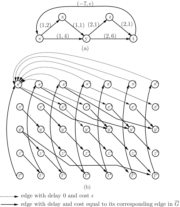
Figure 1: Construction of auxiliary graph $H(v=s)$ with cost constraint $C=6$: (a) graph $\overline{G}$; (b) auxiliary graph $H(v=s)$. The cycle $O=syts$ in $\overline{G}$ is exclude in the auxiliary graph $H(s)$ as shown in (b), keeping the cost of $k$ disjoint paths constrained by $C=6$.

Let $O(v)$ be a cycle in $H(v)$, then following the construction of $H(v)$, $O(v)$ apparently corresponds to a set of cycles in $\overline{G}$. Conversely, every cycle containing $v$ in $\overline{G}$ corresponds to a cycle in $H(v)$. Based on the observation, the following lemma gives the key idea of computing a cycle $O$ of $\overline{G}$ with $\frac{d(O)}{c(O)}$ minimized and cost bounded by $C$:

Lemma 12

Let $O(v_{i})$ be a cycle with minimum $\frac{d(O(v_{i}))}{c(O(v_{i}))}$ in $H(v_{i})$, and $O(v)$ be the cycle with minimum $\frac{d(O(v))}{c(O(v))}$ among the $n$ cycles $O(v_{1}),\dots,O(v_{n})$. Assume $O$ is a cycle with minimum $\frac{d(O)}{c(O)}$ in the set of cycles in $\overline{G}$ that correspond to $O(v)$. Then for any cycle $O^{\prime}$ in $\overline{G}$ with $c(O^{\prime})\leq C$, $\frac{d(O)}{c(O)}\leq\frac{d(O^{\prime})}{c(O^{\prime})}$ holds.

Proof

Suppose this lemma is not true, then there must exist in $\overline{G}$ a cycle, say $O^{\prime}$, such that $\frac{d(O)}{c(O)}>\frac{d(O^{\prime})}{c(O^{\prime})}$ and $c(O^{\prime})\leq C$ hold. Then the cycle $O^{\prime}(v)$ in $H(v)$ that corresponds to $O^{\prime}$ is also with $\frac{d(O^{\prime}(v))}{c(O^{\prime}(v))}=\frac{d(O^{\prime})}{c(O^{\prime})}<\frac{d(O)}{c(O)}\leq\frac{d(O(v))}{c(O(v))}$, contradicting with the minimality of $O(v)$ in $H(v)$. This completes the proof.

3.2 Computing the cycle $O$ with minimum $\frac{d(O)}{c(O)}$

The main idea of the algorithm to compute a cycle $O$ with $\frac{d(O)}{c(O)}$ minimized in $\overline{G}$ is to compute the cycle $O^{\prime}$ with minimum $\frac{d(O^{\prime})}{c(O^{\prime})}$ among all cycles in all $H(v)$s for each $v\in\overline{G}$. Following Lemma 12, the cycle $O$ in $\overline{G}$ is the cycle with minimum $\frac{d(O)}{c(O)}$ among the cycles in $\overline{G}$ corresponding to all the computed $O^{\prime}$s. The detailed steps are as below:

1. For $i=1\,to\,n$

   1. Construct $H(v_{i})$ for $v_{i}\in\overline{G}$ by Algorithm 3;

   2. Compute cycle $O(v_{i})$ with minimum $\frac{d(O(v_{i}))}{c(O(v_{i}))}$ in $H(v_{i})$ by employing the minimum cost-to-time ratio cycle algorithm in [1];

   3. Select $O(v)$ with minimum $\frac{d(O(v))}{c(O(v))}$ from the $n$ computed cycles $O(v_{1}),\dots,O(v_{n})$;

2. Select the cycle $O$ with minimum $\frac{d(O)}{c(O)}$ among the cycles in $\overline{G}$ that correspond to $O(v)$.

Clearly, the cycle $O$ attains minimum $\frac{d(O)}{c(O)}$ in $\overline{G}$. Besides, following Lemma 11 we have $c(O)\leq C$. Therefore the cycle $O$ is correctly the promised cycle. This completes the proof of the approximation ratio.

4 Conclusion

This paper gave a novel approximation algorithm with ratio $(1+\beta,\,\max\{2,\,1+\ln\frac{1}{\beta}\})$ for the $k$BCP problem based on improving a simple $(\alpha,\,2-\alpha)$-approximation algorithm by constructing interesting auxiliary graphs and employing the cycle cancellation method. By setting $\beta=0$, an approximation algorithm with bifactor ratio $(1,\,O(\ln n))$, i.e. an $O(\ln n)$-approximation algorithm can be obtained immediately. To the best of our knowledge, it is the first non-trivial approximation algorithm for this problem that obeys the delay constraint strictly. We are now investigating whether any constant factor approximation algorithm exists for computing a solution that strictly obey the delay constraint.

References

- [1] R.K. Ahuja, T.L. Magnanti, and J.B. Orlin. Network flows: theory, algorithms, and applications. 1993.
- [2] R. Bhatia, M. Kodialam, and TV Lakshman. Finding disjoint paths with related path costs. Journal of Combinatorial Optimization, 12(1):83–96, 2006.
- [3] P. Chao and S. Hong. A new approximation algorithm for computing 2-restricted disjoint paths. IEICE transactions on information and systems, 90(2):465–472, 2007.
- [4] M.R. Garey and D.S. Johnson. Computers and intractability. Freeman San Francisco, 1979.
- [5] L. Guo and H. Shen. On Finding Min-Min disjoint paths. accepted by Algorithmica.
- [6] L. Guo and H. Shen. Efficient approximation algorithms for computing k disjoint minimum cost paths with delay constraint. In PDCAT(2012), IEEE, pages 627–631. IEEE, 2012.
- [7] L. Guo and H. Shen. On the complexity of the edge-disjoint min-min problem in planar digraphs. Theoretical computer science, 432:58–63, 2012.
- [8] C.L. Li, T.S. McCormick, and D. Simich-Levi. The complexity of finding two disjoint paths with min-max objective function. Discrete Applied Mathematics, 26(1):105–115, 1989.
- [9] D.H. Lorenz and D. Raz. A simple efficient approximation scheme for the restricted shortest path problem. Operations Research Letters, 28(5):213–219, 2001.
- [10] A. Orda and A. Sprintson. Efficient algorithms for computing disjoint QoS paths. In IEEE INFOCOM, volume 1, pages 727–738. Citeseer, 2004.
- [11] JW Suurballe. Disjoint paths in a network. Networks, 4(2), 1974.
- [12] JW Suurballe and RE Tarjan. A quick method for finding shortest pairs of disjoint paths. Networks, 14(2), 1984.
- [13] D. Xu, Y. Chen, Y. Xiong, C. Qiao, and X. He. On the complexity of and algorithms for finding the shortest path with a disjoint counterpart. IEEE/ACM Transactions on Networking, 14(1):147–158, 2006.
- [14] G. Xue, W. Zhang, J. Tang, and K. Thulasiraman. Polynomial time approximation algorithms for multi-constrained qos routing. IEEE/ACM Transactions on Networking (TON), 16(3):656–669, 2008.