Slow dynamics of spin pairs in random hyperfine field: Role of inequivalence of electrons and holes in organic magnetoresistance

Abstract

In an external magnetic field B, the spins of the electron and hole will precess in effective fields ${\bm{b}}_{\scriptscriptstyle e}+{\bm{B}}$ and ${\bm{b}}_{\scriptscriptstyle h}+{\bm{B}}$, where ${\bm{b}}_{\scriptscriptstyle e}$ and ${\bm{b}}_{\scriptscriptstyle h}$ are random hyperfine fields acting on the electron and hole, respectively. For sparse “soft” pairs the magnitudes of these effective fields coincide. The dynamics of precession for these pairs acquires a slow component, which leads to a slowing down of recombination. We study the effect of soft pairs on organic magnetoresistance, where slow recombination translates into blocking of the passage of current. It appears that when ${\bm{b}}_{\scriptscriptstyle e}$ and ${\bm{b}}_{\scriptscriptstyle h}$ have identical gaussian distributions the contribution of soft pairs to the current does not depend on $B$. Amazingly, small inequivalence in the rms values of $b_{\scriptscriptstyle e}$ and $b_{\scriptscriptstyle h}$ gives rise to a magnetic field response, and it becomes progressively stronger as the inequivalence increases. We find the expression for this response by performing the averaging over ${\bm{b}}_{\scriptscriptstyle e}$, ${\bm{b}}_{\scriptscriptstyle h}$ analytically. Another source of magnetic field response in the regime when current is dominated by soft pairs is inequivalence of the $g$-factors of the pair partners. Our analytical calculation indicates that for this mechanism the response has an opposite sign.

I Introduction

Due to complex structure of organic semiconductors and their spatial inhomogeneity it is nearly impossible to identify a unique scenario of current passage through them. In view of this, it is remarkable that sizable change of current through a device based on organic semiconductor takes place in weak external magnetic fields. This effect, called organic magnetoresistance (OMAR), seems to be robust, i.e. weakly sensitive to the device parameters. Although the first reports on the observation of organic magnetoresistance (OMAR) appeared decades agofrankevich ; frankevich1 , systematic experimental study of this effect started relatively recently. Markus0 ; Markus1 ; Markus2 ; Markus3 ; Gillin ; Valy0 ; Valy1 ; Valy2 ; Valy3 ; Blum ; Bobbert1 ; Bobbert2 ; Wagemans2 ; Wagemans ; Wagemans1 (see also the review Ref. WagReview, ).

On the theory side, it is now commonly accepted that the origin of OMAR lies in random hyperfine fields created by nuclei surrounding the carriers (polarons). More specifically, the basic unit responsible for OMAR is a pair of sites hosting carriers (polarons); the spin state of the pair is described by the Hamiltonian

$$\widehat{H}={\bm{\Omega}}_{1}\cdot\widehat{{\bm{S}}}_{\scriptscriptstyle e}+{\bm{\Omega}}_{2}\cdot\widehat{{\bm{S}}}_{\scriptscriptstyle h}.$$ (1)

Here $\widehat{{\bm{S}}}_{\scriptscriptstyle e}$ are $\widehat{{\bm{S}}}_{\scriptscriptstyle h}$ are the spin operators of the pair-partners (we will assume that they are electron and hole, respectively); ${\bm{\Omega}}_{1}={\bm{B}}+{\bm{b}}_{\scriptscriptstyle e}$ and ${\bm{\Omega}}_{2}={\bm{B}}+{\bm{b}}_{\scriptscriptstyle h}$ are the full fields acting on the spins. They represent the sums of external, ${\bm{B}}$, and respective hyperfine fields, ${\bm{b}}_{\scriptscriptstyle e}$ and ${\bm{b}}_{\scriptscriptstyle h}$. As was first pointed out by Schulten and Wolynes Schulten , due to the large number of nuclei surrounding each pair-partner and their slow dynamics, ${\bm{b}}_{\scriptscriptstyle e}$ and ${\bm{b}}_{\scriptscriptstyle h}$ can be viewed as classical random fields with gaussian distributions.

In order to give rise to OMAR the Hamiltonian Eq. (1) is not sufficient. It should be complemented by some mechanism through which the pair-partners “know” about each other, so their motion is correlated without direct interaction. The simplest example of such a mechanism is spin-dependent recombination, i.e. the requirement that electron and hole can recombine only if their spins are in the singlet, $S$, state. Then the essence of OMAR can be crudely understood as a redistribution of portions of singlets and triplets upon increasing $B$. This redistribution affects the net recombination rate. Clearly, the characteristic $B$ for this redistribution is $\sim b_{\scriptscriptstyle e},b_{\scriptscriptstyle h}$.

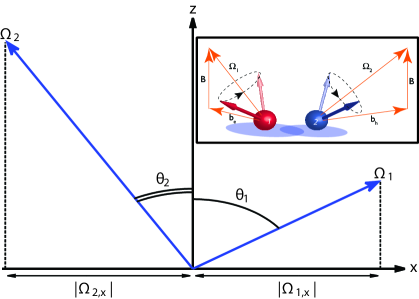
Figure 1: Preferential coordinate system used for analysis of the dynamics of the spin pair. Both fields ${\bm{\Omega}}_{1}$, ${\bm{\Omega}}_{2}$ reside in the $xz$-plane. The direction of the quantization axis, $z$, is fixed by the condition ${\bm{\Omega}}_{1,x}=-{\bm{\Omega}}_{2,x}$.

Naturally, the specific relation between the current and recombination rate involves also the rate at which the pairs are created. It is important, though, that the latter process is not spin-selective.

Existing theories of OMAR can be divided into two groups which we will call “steady-state” and “dynamical”. The theories of the first groupPrigodin appeared earlier. In a nutshell (see Ref. Wagemans, for details), in these theories the right-hand-side of the equation of motion for the density matrix $i\dot{\rho}=[\widehat{H},\rho]$ with Hamiltonian Eq. (1) is complemented with “source” and spin-selective “sink” terms. After that, $\dot{\rho}$ is set to zero. In Refs. Bobbert1, current is expressed via the steady-state $\rho$ and subsequently averaged numerically over realizations of hyperfine fields.

The “steady-state” approach applies when the pair does not perform many beatings between $S$ and $T$ during its lifetime, since the beating dynamics is excluded by setting $\dot{\rho}=0$.

This beating dynamics has been incorporated into the OMAR theory Ref. Flatte1, , which appeared last year. This theory relies on decades old findings in the field of dynamic spin-chemistrySchulten ; reviews . Below we briefly summarize these findings.

If an isolated pair is initially in $S$, it was shown in Ref. Schulten, that the averaged probability to find it in $T$ after time $t$ is given either by the function

$$p_{\scriptscriptstyle ST}(t)=\frac{1}{2}\left(1-e^{-b_{\scriptscriptstyle e}^{2}t^{2}}e^{-b_{\scriptscriptstyle h}^{2}t^{2}}\right),$$ (2)

for strong fields $B\gg b_{\scriptscriptstyle e},b_{\scriptscriptstyle h}$, or by

$$p_{\scriptscriptstyle ST}(t)=\frac{3}{4}\left\{1-\left[\frac{1}{3}\left(1+2e^{-b_{\scriptscriptstyle e}^{2}t^{2}}-4b_{\scriptscriptstyle e}^{2}t^{2}e^{-b_{\scriptscriptstyle e}^{2}t^{2}}\right)\right]\right.\\ \times\left.\left[\frac{1}{3}\left(1+2e^{-b_{\scriptscriptstyle h}^{2}t^{2}}-4b_{\scriptscriptstyle h}^{2}t^{2}e^{-b_{\scriptscriptstyle h}^{2}t^{2}}\right)\right]\right\},$$ (3)

for $B\ll b_{\scriptscriptstyle e},b_{\scriptscriptstyle h}$. Here $b_{\scriptscriptstyle e}$, $b_{\scriptscriptstyle h}$ are the rms hyperfine fields for electron and hole. Naturally, the probability approaches $3/4$ at small $B$ and $1/2$ at large $B$.

In the theory of Ref. Flatte1, the $B$-dependent dynamics described by Eqs. (2), (3) translates into the $B$-dependent resistance (OMAR) on the basis of the following reasoning. The dynamics $p_{\scriptscriptstyle ST}(t)$ leads to prolongation of the recombination time (hopping time, $\tau_{\scriptscriptstyle h}$, in the language of Ref. Flatte1, ). This prolongation is quantified by

$$\frac{1}{\tau_{\scriptscriptstyle h}}\rightarrow\frac{1}{\tau_{\scriptscriptstyle h}}\int dt(1-3p_{\scriptscriptstyle ST}(t))e^{-t/\tau_{\scriptscriptstyle h}}.$$ (4)

The meaning of Eq. (4) is that a pair should stay in $S$ in order for a hop to take place. Prolongation of hopping time leads to a $B$-dependent increase of the resistance. The authors of Ref. Flatte1, evaluated $p_{\scriptscriptstyle ST}(t)$ for arbitrary $B$, while in calculation of OMAR they assumed that bare hopping times, $\tau_{\scriptscriptstyle h}$, have an exponentially broad distribution.

Both theories Refs. Wagemans, , Flatte1, take as a starting point a pair with the Hamiltonian Eq. (1) describing its spin states and preferential recombination (hopping) from $S$. The dynamics of this seemingly simple entity, which is crucial for OMAR, possesses some nontrivial regimes. Uncovering these regimes is a central goal for the present paper. The other goal is to demonstrate that nontrivial dynamics can manifest itself in OMAR.

To underline that the spin dynamics of two carriers in non-collinear magnetic fields which can recombine only from $S$ can be highly nontrivial, we note that separation of this dynamics into $S$-$T$ “beating” stage followed by instantaneous hopping after time $\tau_{\scriptscriptstyle h}$, as in theory Flatte1, , is not always possible. It is quite nontrivial that spin-selective recombination of carriers can exert a feedback on the spin dynamics. As an illustration of this delicate issue we invoke the example of cooperative photon emission discovered by R. H. DickeDicke . In the Dicke effect one superradiant state of a group of emitters having a very short lifetime automatically implies that all the remaining states are subradiant and have anomalously long radiation times. Below we demonstrate that a similar situation is realized in dynamics of two spins when recombination from $S$ is very fast. We will see that the remaining $3$ modes of the collective spin motion become very “slow”.

Our analysis reveals the exceptional role of the “soft” pairs, which are sparse configurations of ${\bm{b}}_{\scriptscriptstyle e}$, ${\bm{b}}_{\scriptscriptstyle h}$ for which full fields ${\bm{\Omega}}_{1}$, ${\bm{\Omega}}_{2}$ have the same magnitude.

The paper is organized as follows. In Sect. II we cast the eigenmodes of the Hamiltonian Eq. (1) in a convenient notation. In Sect. III we include recombination and study its effect on the eigenmodes. The consequences of nontrivial dynamics for OMAR are considered in Sects. IV and V, where we perform averaging over realizations of hyperfine fields. We establish that inequivalence of rms hyperfine fields for electrons and holes has a dramatic effect on OMAR, when it is governed by soft pairs. Sect. VI concludes the paper.

II Dynamics of a pair in the presence of recombination

II.1 Isolated pair

We start with reviewing the dynamics of a pair of spins in the absence of recombination. Obviously, this dynamics does not depend on the choice of the quantization axis. However, since we plan to include recombination, the choice of the quantization axis, $z$, illustrated in Fig. 1 appears to be preferential. The axis is chosen to lie in the plane containing the vectors ${\bm{\Omega}}_{1}$, ${\bm{\Omega}}_{2}$. Moreover, the orientation of the $z$-axis is fixed by the condition ${\bm{\Omega}}_{1x}=-{\bm{\Omega}}_{2x}$. Then the angles, $\theta_{1}$, $\theta_{2}$, between ${\bm{\Omega}}_{1}$, ${\bm{\Omega}}_{2}$ and the $z$-axis are given by

$$\tan\theta_{1}=\frac{|{\bm{\Omega}}_{1}\times{\bm{\Omega}}_{2}|}{{\bm{\Omega}}_{2}^{2}+{\bm{\Omega}}_{1}\cdot{\bm{\Omega}}_{2}},~{}~{}~{}\tan\theta_{2}=\frac{|{\bm{\Omega}}_{1}\times{\bm{\Omega}}_{2}|}{{\bm{\Omega}}_{1}^{2}+{\bm{\Omega}}_{1}\cdot{\bm{\Omega}}_{2}}$$ (5)

With this choice, the Schrödinger equation for the amplitudes of $S$, $T_{0}$, $T_{+}$, and $T_{-}$ reduces to the system

$$i\frac{\partial T_{+}}{\partial t} =\Sigma_{z}T_{+}-\frac{1}{\sqrt{2}}\Delta_{x}S,$$ (6)

$$i\frac{\partial S}{\partial t} =\Delta_{z}T_{0}-\frac{1}{\sqrt{2}}\Delta_{x}T_{+}+\frac{1}{\sqrt{2}}\Delta_{x}T_{-},$$ (7)

$$i\frac{\partial T_{0}}{\partial t} =\Delta_{z}S,$$ (8)

$$i\frac{\partial T_{-}}{\partial t} =-\Sigma_{z}T_{-}+\frac{1}{\sqrt{2}}\Delta_{x}S,$$ (9)

where $\Sigma_{z},\Delta_{z},$ and $\Delta_{x}$ are defined as

$$\Sigma_{z} =\frac{\Omega_{1z}+\Omega_{2z}}{2},$$ (10)

$$\Delta_{z} =\frac{\Omega_{1z}-\Omega_{2z}}{2},$$ (11)

$$\Delta_{x} =\frac{\Omega_{1x}-\Omega_{2x}}{2}.$$ (12)

The advantage of our choice of the quantization axis shows in the fact that the state $T_{0}$ is coupled exclusively to $S$. Since recombination is allowed only from $S$, this will simplify the subsequent analysis of the recombination dynamics.

The eigenvalues, $\lambda_{i}$, of the system Eqs. (6)-(9) satisfy the quartic equation

$$\lambda_{i}^{2}(\lambda_{i}^{2}-\Sigma_{z}^{2})-\lambda_{i}^{2}(\Delta_{z}^{2}+\Delta_{x}^{2})+\Delta_{z}^{2}\Sigma_{z}^{2}=0.$$ (13)

We will enumerate these eigenvalues according to the convention $\lambda_{1}=-\lambda_{2}$ and $\lambda_{3}=-\lambda_{4}$. To find the absolute values $\lambda_{1}^{2}$, $\lambda_{3}^{2}$ one does not have to solve Eq. (13), since it is obvious that for non-interacting spins the eigenvalues are the sums and the differences of individual Zeeman energies

$$\lambda_{1}^{2}=\left(\frac{|{\bm{\Omega}}_{1}|+|{\bm{\Omega}}_{2}|}{2}\right)^{2},~{}~{}\lambda_{3}^{2}=\left(\frac{|{\bm{\Omega}}_{1}|-|{\bm{\Omega}}_{2}|}{2}\right)^{2}.$$ (14)

Naturally, $\lambda_{1}$, $\lambda_{3}$ do not depend on the choice of the quantization axis. At the same time, the coefficients in Eq. (13) do depend on this choice. To trace how the dependence on the quantization axis disappears in the roots of Eq. (13), one should use the following identities

$$\Sigma_{z}^{2}+\Delta_{z}^{2}+\Delta_{x}^{2} =\frac{|{\bm{\Omega}}_{1}|^{2}+|{\bm{\Omega}}_{2}|^{2}}{2},$$ (15)

$$\Sigma_{z}^{2}\Delta_{z}^{2} =\left(\frac{|{\bm{\Omega}}_{1}|^{2}-|{\bm{\Omega}}_{2}|^{2}}{4}\right)^{2}.$$ (16)

In terms of the angles $\theta_{1}$ and $\theta_{2}$, Fig. 1, the corresponding eigenvectors can be expressed as

$$\begin{pmatrix}T_{+}\\ S\\ T_{0}\\ T_{-}\end{pmatrix}=\left\{\begin{pmatrix}\cos\frac{\theta_{1}}{2}\cos\frac{\theta{2}}{2}\\ -\frac{1}{\sqrt{2}}\sin\frac{\theta_{1}+\theta_{2}}{2}\\ \frac{1}{\sqrt{2}}\sin\frac{\theta_{1}-\theta_{2}}{2}\\ -\sin\frac{\theta_{1}}{2}\sin\frac{\theta_{2}}{2}\end{pmatrix},\begin{pmatrix}-\sin\frac{\theta_{1}}{2}\sin\frac{\theta_{2}}{2}\\ -\frac{1}{\sqrt{2}}\sin\frac{\theta_{1}+\theta_{2}}{2}\\ -\frac{1}{\sqrt{2}}\sin\frac{\theta_{1}-\theta_{2}}{2}\\ \cos\frac{\theta_{1}}{2}\cos\frac{\theta{2}}{2}\end{pmatrix},\right.\\ \left.\begin{pmatrix}\cos\frac{\theta_{1}}{2}\sin\frac{\theta{2}}{2}\\ \frac{1}{\sqrt{2}}\cos\frac{\theta_{1}+\theta_{2}}{2}\\ \frac{1}{\sqrt{2}}\cos\frac{\theta_{1}-\theta_{2}}{2}\\ \sin\frac{\theta_{1}}{2}\cos\frac{\theta_{2}}{2}\end{pmatrix},\begin{pmatrix}-\sin\frac{\theta_{1}}{2}\cos\frac{\theta{2}}{2}\\ -\frac{1}{\sqrt{2}}\cos\frac{\theta_{1}+\theta_{2}}{2}\\ \frac{1}{\sqrt{2}}\cos\frac{\theta_{1}-\theta_{2}}{2}\\ -\cos\frac{\theta_{1}}{2}\sin\frac{\theta_{2}}{2}\end{pmatrix}\right\},$$ (17)

where the first two correspond to $\lambda_{1,2}$ while the last two correspond to $\lambda_{3,4}$, respectively.

The form Eq. (17) allows us to make the following observation. When the full magnetic fields acting on spins incidentally coincide, we have $|\bm{\Omega}_{1}|=|\bm{\Omega}_{2}|$. Then it follows from Eq. (14) that $\lambda_{3}=\lambda_{4}=0$, so that the two corresponding eigenstates become degenerate. Under this condition we also have $\theta_{1}=\theta_{2}$. Then the first two eigenvectors Eq. (17) have zeros in the rows corresponding to $T_{0}$. Concerning the other two eigenvectors, due to their degeneracy, their sum and difference are also eigenvectors. The difference has a zero in the row corresponding to $T_{0}$, while the sum consists of the $T_{0}$ component, exclusively. Then we conclude that for realizations of hyperfine field for which $|\bm{\Omega}_{1}|=|\bm{\Omega}_{2}|$ the state $T_{0}$ is completely decoupled from the other three states. This fact has important implications for recombination dynamics, as we will see below.

Including recombination requires the analysis of the full equation for the density matrix

$$i\dot{\rho}=[\widehat{H},\rho]-\frac{i}{2\tau}\left\{\rho,\left|{S}\right>\left<{S}\right|\right\},$$ (18)

where $\tau$ is the recombination time. The form of the second term ensures that recombination takes place only from $S$. The matrix corresponding to Eq. (18) is $16\times 16$. The $16$ eigenvalues can be cast in the form $\lambda_{i}-\lambda_{j}^{\ast}$, where $\lambda_{i}$ and $\lambda_{j}$ satisfy the equation

$$\lambda_{i}\left(\lambda_{i}+\frac{i}{\tau}\right)(\lambda_{i}^{2}-\Sigma_{z}^{2})-\lambda_{i}^{2}(\Delta_{z}^{2}+\Delta_{x}^{2})+\Delta_{z}^{2}\Sigma_{z}^{2}=0.$$ (19)

The latter equation expresses the condition that $\lambda_{i}$ are the eigenvalues of non-hermitian operator $\widehat{H}-\frac{i}{\tau}\left|{S}\right>\left<{S}\right|$. In the limit $\tau\rightarrow\infty$ this equation reduces to Eq. (14). The dynamics of recombination is governed by the imaginary parts of the roots of Eq. (19), i.e. decay is described by the exponents $\exp\left[-\left(\text{Im}\,\lambda_{i}+\text{Im}\,\lambda_{j}\right)t\right]$. Less trivial is that finite $\tau$ can strongly affect the real parts of $\lambda_{i}$. Physically, the dependence of $\text{Re}\,\lambda_{i}$ on $\tau$ describes the back-action of recombination on the dynamics of beating between different eigenstates. In the following two subsections this effect will be analyzed in detail in the two limiting cases.

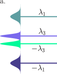
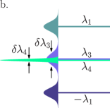
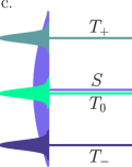
Figure 2: (Color online). (a) Slow-recombination regime, $\Omega_{1,2}\ll 1/\tau$. Horizontal lines represent the energy levels Eq. (14) of a pair in the absence of recombination. Recombination from $S$ causes the broadening of the levels Eqs. (21,22), which, for a typical pair, is of the same order for all levels. (b) Slow-recombination regime. For soft pairs, $|{\bm{\Omega}}_{1}|\approx|{\bm{\Omega}}_{2}|$, recombination results in splitting Eq. (24) of the widths of the levels $\lambda_{3,4}$ rather than their positions. (c) Fast-recombination regime, $\Omega_{1,2}\gg 1/\tau$. The eigenstates $S$, $T_{0}$, $T_{\scriptscriptstyle+}$, and $T_{\scriptscriptstyle-}$ are well-defined. Recombination causes strong broadening, $1/\tau$, of the level $S$, and weak broadening $\sim\Omega_{1,2}^{2}\tau$ of the other three levels.

II.2 Slow Recombination

Consider the limit $1/\tau\ll\lambda_{i}$. In this limit recombination amounts to the small corrections to the bare values of $\lambda_{i}$ given by Eq. (14). This allows one to set $\lambda_{i}$ equal to their bare values in all terms in Eq. (19) containing $1/\tau$, and search for solution in the form $\lambda_{i}+\delta\lambda_{i}$. Then one gets the following expression for the correction $\delta\lambda_{i}$

$$\delta\lambda_{i}=\frac{-i}{\tau}\,\frac{\lambda_{i}(\lambda_{i}^{2}-\Sigma_{z}^{2})}{\lambda_{i}^{3}-2\lambda_{i}(\Sigma_{z}^{2}+\Delta_{z}^{2}+\Delta_{x}^{2})}=\frac{-i}{2\tau}\,\frac{\lambda_{i}^{2}(\lambda_{i}^{2}-\Sigma_{z}^{2})}{\lambda_{i}^{4}-\Sigma_{z}^{2}\Delta_{z}^{2}}.$$ (20)

In the last identity we have used the fact that $\lambda_{i}$ satisfy the equation Eq. (14). The above expression can be greatly simplified with the help of the relations Eq. (15). One has

$$\delta\lambda_{1,2} =-\frac{i}{4\tau}\left(1-\frac{\bm{\Omega}_{1}\cdot\bm{\Omega}_{2}}{|{\bm{\Omega}}_{1}||{\bm{\Omega}}_{2}|}\right),$$ (21)

$$\delta\lambda_{3,4} =-\frac{i}{4\tau}\left(1+\frac{\bm{\Omega}_{1}\cdot\bm{\Omega}_{2}}{|{\bm{\Omega}}_{1}||{\bm{\Omega}}_{2}|}\right).$$ (22)

The above result suggests that for generic mutual orientations of ${\bm{\Omega}}_{1}$ and ${\bm{\Omega}}_{2}$ all modes of a pair decay with characteristic time $\sim\tau$. At the same time, for parallel orientations of ${\bm{\Omega}}_{1}$, ${\bm{\Omega}}_{2}$ the modes $\lambda_{1,2}$ have anomalously long lifetime. This long lifetime has its origin in the fact that for ${\bm{\Omega}}_{1}\parallel{\bm{\Omega}}_{2}$, the states $T_{+}$ and $T_{-}$, which are orthogonal to $S$, are the eigenstates of the Hamiltonian Eq. (1). Formally this can be seen from the general expression Eq. (17) for the eigenvectors upon setting $\theta_{1}=\theta_{2}=0$. Similarly, for ${\bm{\Omega}}_{1}$ and ${\bm{\Omega}}_{2}$ being antiparallel, one can check from Eq. (17) that for $\theta_{1}=\pi-\theta_{2}$, the eigenstates $\lambda_{3}$, $\lambda_{4}$ have no $S$ component, so they are long-lived. Note that the existence of long lifetimes for parallel and antiparallel configurations of ${\bm{\Omega}}_{1}$, ${\bm{\Omega}}_{2}$ is at the core of the “blocking mechanism” of OMAR proposed in Ref. Bobbert1, .

II.2.1 Soft pairs

As was pointed out in the Introduction, recombination also has a pronounced effect on the spin dynamics for sparse configurations for which $|\Omega_{1}|\approx|\Omega_{2}|$. Indeed, for these configurations, the values $\lambda_{3}$ and $\lambda_{4}$ are anomalously small. Then the basic condition, $1/\tau\ll\lambda_{i}$, under which Eq. (21) was derived, is not satisfied. We dub such realizations as soft pairs. For soft pairs the expressions for $\delta\lambda_{1}$, $\delta\lambda_{2}$ remain valid, but the eigenvalues $\lambda_{3}$, $\lambda_{4}$ get strongly modified due to finite recombination time, $\tau$.

Although for soft pairs the terms $\propto 1/\tau$ in Eq. (19) cannot be treated as a perturbation, a different simplification becomes possible in this case. We can neglect $\lambda_{i}^{2}$ compared to $\Sigma_{z}^{2}$ in the first term and $\Delta_{z}^{2}$ compared to $\Delta_{x}^{2}$ in the second term. The first simplification is justified, since the typical value of $\Sigma_{z}$ is $\sim|{\bm{\Omega}}_{1}|\approx|{\bm{\Omega}}_{2}|$ and is much bigger than both $1/\tau$ and $(|{\bm{\Omega}}_{1}|-|{\bm{\Omega}}_{2}|)$. Concerning the second simplification, the smallness of $(|{\bm{\Omega}}_{1}|-|{\bm{\Omega}}_{2}|)$ automatically implies that $\Delta_{z}$ given by Eq. (10) is small. With the above simplifications the eigenvalues $\lambda_{3,4}$ satisfy the quadratic equation

$$(\Sigma_{z}^{2}+\Delta_{x}^{2})\lambda_{i}^{2}+\frac{i}{\tau}\Sigma_{z}^{2}\lambda_{i}-\Delta_{z}^{2}\Sigma_{z}^{2}=0.$$ (23)

Already from the form of Eq. (23) one can make a surprising observation that, even with finite $1/\tau$, one of the roots is identically zero when $\Delta_{z}=0$, i.e. when $|{\bm{\Omega}}_{1}|$ and $|{\bm{\Omega}}_{2}|$ are exactly equal to each other. This suggests that a pair in the state corresponding to this root will never recombine. For a small but finite difference $(|{\bm{\Omega}}_{1}|-|{\bm{\Omega}}_{2}|)$ the recombination will eventually take place but only after time much longer than $\tau$. Indeed, for the generic case, $|{\bm{\Omega}}_{1}|\sim|{\bm{\Omega}}_{2}|)$, we have from Eq. (23)

$$\lambda_{3,4}=-\frac{i}{2\tau}\Bigl{[}\Lambda\pm\sqrt{\Lambda^{2}-4\Lambda\Delta_{z}^{2}\tau^{2}}\Bigr{]},$$ (24)

where the dimensionless parameter $\Lambda$ is defined as

$$\Lambda=\frac{\Sigma_{z}^{2}}{\Sigma_{z}^{2}+\Delta_{x}^{2}}.$$ (25)

Even when $|{\bm{\Omega}}_{1}|$ and $|{\bm{\Omega}}_{2}|$ are close, a typical value of parameter $\Lambda$ is $\sim 1$. Then Eq. (24) suggests that anomalously long-living mode exists in the domain $\Delta_{z}\lesssim 1/\tau$ where its lifetime is $\sim 1/\Delta_{z}^{2}\tau$. Note that the lifetime becomes longer with a decrease of the recombination time.

As the difference $|{\bm{\Omega}}_{1}|-|{\bm{\Omega}}_{2}|$ increases, the product $\Delta_{z}\tau$ becomes big and the expression under the square root in Eq. (24) becomes negative. Then the lifetimes of of both states corresponding to $\lambda_{3}$ and $\lambda_{4}$ become equal to $\tau/\Lambda$. Note that, at the same time, the splitting of the real parts of $\lambda_{3}$ and $\lambda_{4}$ becomes $\sim\Delta_{z}^{2}\tau$, which is much bigger than $|{\bm{\Omega}}_{1}|-|{\bm{\Omega}}_{2}|$.

The above effect can be interpreted as a repulsion of the eigenvalues caused by recombinationGefen . A more prominent analogy can be found in opticsDicke . The signs $+$ and $-$ in Eq. (24) can be related to the superradiant and subradiant modes of two identical emitters. The role of $\tau$ in this case is played by their radiative lifetime.

Both effects illustrate the back-action of recombination on the dynamics of the pair when the spin levels of pair-partners are nearly degenerate. To track an analogy to this effect one can refer to Refs. subradiance1, and subradiance2, , where Eq. (24) appeared in connection to resonant tunneling through a pair of nearly degenerate levels, while the role of $1/\tau$ was played by the level width with respect to escape into the leads.

For our choice of the quantization axis the long-living state corresponds to $T_{0}$. For completeness we rewrite the parameter $\Delta_{z}$, which enters Eq. (24), in the coordinate-independent form

$$\Delta_{z}^{2}=\frac{(|{\bm{\Omega}}_{1}|^{2}-|{\bm{\Omega}}_{2}|^{2})^{2}}{4|{\bm{\Omega}}_{1}+{\bm{\Omega}}_{2}|^{2}}.$$ (26)

To establish coordinate-independent form of parameter $\Lambda$ we need the combinations $\Sigma_{z}^{2}$ and $\Sigma_{z}^{2}+\Delta_{x}^{2}$, which are given by

$$\Sigma_{z}^{2} =\frac{|{\bm{\Omega}}_{1}+{\bm{\Omega}}_{2}|^{2}}{4},$$ (27)

$$\Sigma_{z}^{2}+\Delta_{x}^{2} =\frac{|{\bm{\Omega}}_{1}|^{2}+|{\bm{\Omega}}_{2}|^{2}}{2}-\frac{\left(|{\bm{\Omega}}_{1}|^{2}-|{\bm{\Omega}}_{2}|^{2}\right)^{2}}{4|{\bm{\Omega}}_{1}+{\bm{\Omega}}_{2}|^{2}},$$ (28)

so that $\Lambda$ can be cast into the form

$$\Lambda=\frac{|{\bm{\Omega}}_{1}+{\bm{\Omega}}_{2}|^{4}}{|{\bm{\Omega}}_{1}+{\bm{\Omega}}_{2}|^{4}+4|{\bm{\Omega}}_{1}\times{\bm{\Omega}}_{2}|^{2}}.$$ (29)

The consequences of “trapping” described by Eq. (24) for OMAR will be considered in Sections IV and V. In the subsequent subsection we will see that the similar physics, namely, the emergence of slow modes due to fast recombination persists also in the domain $|{\bm{\Omega}}_{1,2}|\tau\ll 1$.

II.3 Fast Recombination

In the opposite limit, $\tau\ll|{\bm{\Omega}}_{1,2}|^{-1}$, the bracket $(\lambda_{i}+\frac{i}{\tau})$ in Eq. (19) is big. This suggests that three zero-order eigenvalues are

$$\lambda_{i}=0,\pm\Sigma_{z}.$$ (30)

In the same order, the fourth eigenvalue is $-\frac{i}{\tau}$. Concerning the eigenvectors, in the zeroth order they are simply $S,T_{+},T_{-},$ and $T_{0}$. This follows from the equation

$$i\dot{S}+\frac{i}{\tau}S=\Delta_{z}T_{0}-\frac{1}{\sqrt{2}}T_{+}+\frac{1}{\sqrt{2}}T_{-}.$$ (31)

Taking $\tau$ to zero means that in the zeroth order $S=0$. Then three other equations in the system Eq. (6) get decoupled.

In the first order, the eigenvalues Eq. (30) acquire imaginary parts

$$\delta\lambda_{i}=-i\tau\left(\frac{\lambda_{i}^{2}(\Delta_{z}^{2}+\Delta_{x}^{2})-\Delta_{z}^{2}\Sigma_{z}^{2}}{3\lambda_{i}^{2}-\Sigma_{z}^{2}}\right).$$ (32)

With the help of Eqs. (27) and (29) these imaginary parts can be simplified to

$$\delta\lambda_{T_{0}} =-i\tau\Delta_{z}^{2}=-i\tau\frac{(\Omega_{1}^{2}-\Omega_{2}^{2})^{2}}{4|\bm{\Omega}_{1}+\bm{\Omega}_{2}|^{2}},$$ (33)

$$\delta\lambda_{T_{+}}=\delta\lambda_{T_{-}} =-i\tau\frac{\Delta_{x}^{2}}{2}=-i\tau\frac{|\bm{\Omega}_{1}\times\bm{\Omega}_{2}|^{2}}{2|\bm{\Omega}_{1}+\bm{\Omega}_{2}|^{2}}.$$ (34)

We see that for a generic situation $|\bm{\Omega}_{1}|\sim|\bm{\Omega}_{2}|$ the lifetime of the modes $T_{0}$, $T_{+}$, and $T_{-}$ are $\sim 1/|\bm{\Omega}_{1,2}|^{2}\tau$, i.e. in the regime of fast recombination it is much longer than $\tau$. This is a consequence of effective decoupling of $T_{0}$, $T_{+}$, and $T_{-}$ from $S$ in this regime. We also observe from Eq. (33) that there is additional prolongation of lifetime for the mode $T_{0}$ if the pair is soft. Eq. (33) also suggests that lifetimes of the states $T_{+}$, $T_{-}$ are anomalously long when $\bm{\Omega}_{1}$ and $\bm{\Omega}_{2}$ are collinear. This expresses the obvious fact that, for collinear effective fields acting on the pair-partners, $T_{+}$ and $T_{-}$ are the eigenstates no matter whether recombination is present or not.

Once the eigenvalues and eigenvectors of a pair in the presence of recombination are established, the next question crucial for transport through the pair is: Suppose that initial state is a random superposition of $S$, $T_{0}$, $T_{+}$, and $T_{-}$, what is the average (over the coefficients of superposition) waiting time for this state to recombine? Naturally, the answer to this question does not depend on the actual choice of the orthonormal basis. We address this question in the next section.

III Recombination time from a random initial state

III.1 Soft pair in a slow recombination regime

To illustrate the peculiarity of the question posed above, we start from an instructive particular case of soft pair in a slow recombination regime. We defined a soft pair as a pair for which the condition $(|{\bm{\Omega}}_{1}|-|{\bm{\Omega}}_{2}|)\ll|{\bm{\Omega}}_{1,2}|$ is met. However, in the slow recombination regime, the combination $(|{\bm{\Omega}}_{1}|-|{\bm{\Omega}}_{2}|)\tau$ can be either big or small. In both cases there is a strong separation between the absolute values of $\lambda_{1,2}$ and $\lambda_{3,4}$. It can be seen from Eq. (24) that in the limit $(|{\bm{\Omega}}_{1}|-|{\bm{\Omega}}_{2}|)\tau\gg 1$, the recombination times for states which correspond to $\lambda_{3}$ and $\lambda_{4}$ are given by

$$t_{\scriptscriptstyle R}^{\scriptscriptstyle(3)}=\frac{2\tau}{\Lambda}~{}~{}~{}\text{and}~{}~{}~{}t_{\scriptscriptstyle R}^{\scriptscriptstyle(4)}=\frac{2\tau}{\Lambda},$$ (35)

while in the opposite limit, $(|{\bm{\Omega}}_{1}|-|{\bm{\Omega}}_{2}|)\tau\ll 1$, we get

$$t_{\scriptscriptstyle R}^{\scriptscriptstyle(3)}=\frac{2\tau}{\Lambda}~{}~{}~{}\text{and}~{}~{}~{}t_{\scriptscriptstyle R}^{\scriptscriptstyle(4)}=\frac{1}{\tau\Delta_{z}^{2}}.$$ (36)

We see that the recombination time of $\lambda_{3}$ is $\sim\tau$ for both limits, while the recombination time of $\lambda_{4}$ crosses over from $\sim\tau$ to $\sim 1/\Delta_{z}^{2}\tau$ as $(|{\bm{\Omega}}_{1}|-|{\bm{\Omega}}_{2}|)\tau$ decreases. Taking into account that for generic case $|{\bm{\Omega}}_{1}|\sim|{\bm{\Omega}}_{2}|$ the recombination times corresponding to $\lambda_{1,2}$ are $\sim\tau$, we conclude that for purely random initial conditions the average recombination time is either $\sim\tau$ or it is $\frac{1}{4}$ of $1/\Delta_{z}^{2}\tau$.

The major complication for getting exact average recombination time for a soft pair is that the exact eigenstates represent mixtures with weights governed by the recombination time. This follows from Eq. (24). In addition, the eigenstates corresponding to $\lambda_{3}$, and $\lambda_{4}$ are not orthogonal to each other. However, for a soft pair these complications can be overcome. The reason is that, there are two small parameters in the problem, $1/\tau|{\bm{\Omega}}_{1,2}|$, and $(|{\bm{\Omega}}_{1}|-|{\bm{\Omega}}_{2}|)/|{\bm{\Omega}}_{1,2}|$. The first parameter guarantees slow recombination, while the second ensures that the pair is soft. The presence of these parameters allows us to evaluate $\langle t_{\scriptscriptstyle R}\rangle$ in the closed form using the general formula

$$\langle t_{\scriptscriptstyle R}\rangle=\frac{1}{4}\sum_{i,j}g_{ji}(g^{-1}_{ji})^{*}\frac{1}{i(\lambda_{i}-\lambda_{j}^{*})},$$ (37)

where $g_{ij}=\left<v_{i}|v_{j}\right>$ is a matrix of inner products of eigenvectors corresponding to complex eigenvalues $\lambda_{i}$ and $\lambda_{j}$. The above formula becomes absolutely transparent when the eigenvectors are orthonormal. Then the matrix $g_{ij}$ reduces to the Kronecker symbol, $\delta_{ij}$, and $\langle t_{\scriptscriptstyle R}\rangle$ simplifies to

$$\langle t_{\scriptscriptstyle R}\rangle=-\frac{1}{8}\sum_{j}\frac{1}{\text{Im}\,\lambda_{j}},$$ (38)

which expresses the fact that for random initial state the average recombination time is the evenly-weighted sum of recombination times from eigenstates.

In the case of a soft pair and slow recombination one should use Eq. (37) to evaluate $\langle t_{\scriptscriptstyle R}\rangle$. What enables this evaluation is that, by virtue of small parameters, the eigenvectors corresponding to $\lambda_{1}$ and $\lambda_{2}$ are mutually orthogonal (with accuracy $1/\tau|{\bm{\Omega}}_{1,2}|$), and they are both orthogonal to eigenvectors corresponding to $\lambda_{3}$ and $\lambda_{4}$. Therefore, in evaluating Eq. (37), one has to deal only with mutual non-orthogonality of two eigenvectors $v_{3}$ and $v_{4}$. The straightforward calculation yields

$$\langle t_{\scriptscriptstyle R}\rangle=\frac{\tau}{\Lambda}+\frac{1}{4\Delta_{z}^{2}\tau}-\frac{1}{\text{Im}\,\lambda_{1}}-\frac{1}{\text{Im}\,\lambda_{2}},$$ (39)

where ${\text{Im}\,\lambda_{1}}={\text{Im}\,\lambda_{2}}$ are given by Eq. (21). It is easy to see that in the limiting cases of large and small $(|{\bm{\Omega}}_{1}|-|{\bm{\Omega}}_{2}|)\tau$ Eq. (39) reproduces Eqs. (35) and (36), respectively.

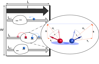
Figure 3: (Color online). The simplest model of transport through a bipolar device in which the currents flow along independent chains. Electrons arrive at the recombination region from the left, while the holes arrive from the right. Blobs enclose the sites from which electron and hole recombine. One of the blobs is enlarged to illustrate the spin precession of the pair partners in their respective fields ${\bm{\Omega}}_{1}$, ${\bm{\Omega}}_{2}$. For soft pairs the magnitudes of ${\bm{\Omega}}_{1}$ and ${\bm{\Omega}}_{2}$ are close to each other.

While in the last two terms in Eq. (39) depend weakly on the degree of “softness” of the pair, $\Delta_{z}\propto(|{\bm{\Omega}}_{1}|-|{\bm{\Omega}}_{2}|)$, the second term exhibits unlimited growth with decreasing $\Delta_{z}$. We emphasize the peculiarity of this situation. In conventional quantum mechanics, when the level separation becomes smaller than their width, it should be simply replaced by the width. What makes Eq. (39) special is that the smaller is $\Delta_{z}$ the more the state $T_{0}$ becomes isolated. There is direct analogy of this situation with the Dicke effectDicke , as was mentioned in the Introduction. By virtue of this analogy, the state $T_{0}$ assumes the role of the “subradiant” mode which accompanies the formation of the superradiant mode. In the Dicke effect the formation of superradiant and subradiant states occurs because the bare states are coupled via continuum. In our situation it is recombination that is responsible for “isolation” of $T_{0}$. If the pair is not soft, the calculation of the time $\langle t_{\scriptscriptstyle R}\rangle$ in the slow-hopping regime can be performed by simply using Eq. (38) and $\lambda_{i}$ given by Eqs. (21), (24). This is because the smallness of $1/\tau$ makes the eigenstates almost orthogonal. However, the Dicke physics becomes even more pronounced in the fast-recombination regime, as demonstrated in the next subsection.

III.2 Recombination time in the fast recombination regime

It might seem that under the condition of fast recombination $|{\bm{\Omega}}_{1,2}|\tau\ll 1$ the recombination time from the random initial state should be $\sim\tau$, since spins practically do not precess during the time $\tau$. The fact that recombination takes place only from $S$, while initial state is a random mixture, already suggests that $\langle t_{\scriptscriptstyle R}\rangle$ is longer than $\tau$. This is because if the initial configuration is different from $S$ it must first cross over into $S$ by spin precession before it recombines. The characteristic time for the spin precession is $\sim|{\bm{\Omega}}_{1,2}|^{-1}\gg\tau$. It turns out that the crossing time is actually much longer than $|{\bm{\Omega}}_{1,2}|^{-1}$. Formally, this fact follows from Eqs. (33), (34) for $\delta\lambda_{i}$, which are of the order of $|{\bm{\Omega}}_{1,2}|^{2}\tau$ rather than $|{\bm{\Omega}}_{1,2}|$. We can now interpret this result by identifying $S$ with superradiant state, while $T_{0}$, $T_{+}$, and $T_{-}$ assume the roles of subradiant states. The short lifetime of $S$ isolates it from the rest of the system. Quantitatively, the portion of $S$ in the other eigenvectors is $\sim|{\bm{\Omega}}_{1,2}|\tau$.

What is important for calculation of $\langle t_{\scriptscriptstyle R}\rangle$ is the fact that eigenvectors are orthogonal (with accuracy $\sim 1/|{\bm{\Omega}}_{1,2}|\tau$) in the fast-recombination regime. This allows one to replace the overlap integrals $g_{\scriptscriptstyle ij}$ in Eq. (37) by $\delta_{\scriptscriptstyle ij}$ and use the Eq. (38) which immediately yields for $\langle t_{\scriptscriptstyle R}\rangle$ the result

$$\langle t_{\scriptscriptstyle R}\rangle =-\frac{1}{8}\left(\frac{1}{\text{Im}\,\lambda_{S}}+\frac{1}{\text{Im}\,\lambda_{T_{0}}}+\frac{1}{\text{Im}\,\lambda_{T_{+}}}+\frac{1}{\text{Im}\,\lambda_{T_{-}}}\right)$$ (40)

$$=\frac{1}{8}\left[\tau+\frac{1}{\tau}\left(\frac{1}{\Delta_{z}^{2}}+\frac{4}{\Delta_{x}^{2}}\right)\right].$$ (41)

Substituting the coordinate-independent expressions for $\Delta_{x}$ and $\Delta_{z}$, we arrive at the final expression for recombination time, which is applicable within the entire fast-recombination regime

$$\langle t_{\scriptscriptstyle R}\rangle=\frac{1}{8}\left[\tau+\frac{4}{\tau}\left(\frac{|{\bm{\Omega}}_{1}+{\bm{\Omega}}_{2}|^{2}}{\left(|{\bm{\Omega}}_{1}|^{2}-|{\bm{\Omega}}_{2}|^{2}\right)^{2}}+\frac{|{\bm{\Omega}}_{1}+{\bm{\Omega}}_{2}|^{2}}{|{\bm{\Omega}}_{1}\times{\bm{\Omega}}_{2}|^{2}}\right)\right].$$ (42)

As was already noticed in the previous section, recombination time diverges for two particular configurations: soft pairs with $|{\bm{\Omega}}_{1}|=|{\bm{\Omega}}_{2}|$ and collinear ${\bm{\Omega}}_{1}$ and ${\bm{\Omega}}_{2}$. Certainly this divergence will be cut off in the course of calculation of current through a pair to which we now turn.

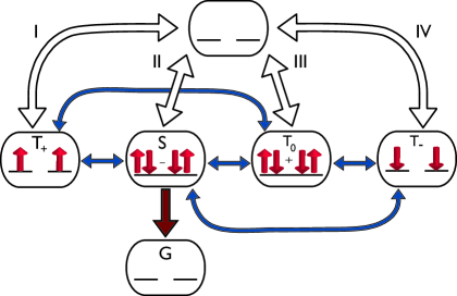
Figure 4: (Color online). I, II, III, and IV are possible variants of the current cycle. For each variant the pair is initially created in one of four states. This is followed by time evolution, illustrated by blue double arrows, which mixes the states. Subsequently, the pair either recombines from $S$ (brown arrow) or dissociates. The processes of creation and dissociation are indicated by white double arrows. The current is the inverse duration, $\overline{t}$, of the cycle averaged over initial states, which we assume to have equal probabilities. The time, $\overline{t}$, is given by Eqs. (44), (45), or (46) depending on the recombination regime.

IV Transport model

We adopt a transport model illustrated in Fig. 3. For concreteness we will discuss a bipolar device, so that the current is due to electron-hole recombination. As shown in Fig. 3, electrons arrive at the pair of sites (enlarged regions in Fig. 3) from the left, while holes arrive from the right. Once an electron-hole pair is formed, the spins of the pair-partners undergo precession in the fields ${\bm{\Omega}}_{1}$ and ${\bm{\Omega}}_{2}$, respectively, waiting to either recombine or to bypass each other and proceed along their respective current paths. For simplicity we choose the current paths in the form of $1D$ chains. This choice makes the adopted model of transport very close to the “two-site” model proposed in Ref. Bobbert1, . The on-site dynamics of a pair with recombination was studied in detail in previous sections. To utilize the results of Sect. III for the calculation of current, $I$, one has to incorporate the stages of formation and dissociation of pairs into the description of transport.

In Fig. 4 the formation and dissociation are illustrated with white double-sided arrows. The formation time for all four variants of initial states is assumed to be the same, $\tau_{\scriptscriptstyle D}$. For simplicity we choose the average time for bypassing to be also $\tau_{\scriptscriptstyle D}$. Note that this choice does not limit the generality of the description, provided that $\tau_{\scriptscriptstyle D}$ is longer than the recombination time. The middle and the bottom portions in Fig. 4 illustrate the spin precession (blue arrows) and recombination (brown arrow) stages, which we studied earlier. Implicit in Fig. 4, is that the pair disappears either due to dissociation or by recombination before the next charge carrier arrives. Another way to express this fact is to state that the passage of current proceeds in cycles.

Naturally, subsequent cycles are statistically independent. This allows one to express the current along a $1D$ path through the average duration of the cycle, $\overline{t}$. Indeed, $N\gg 1$ cycles take the time $T_{\scriptscriptstyle N}=t_{1}+t_{2}+\cdots+t_{\scriptscriptstyle n}$. For large $N$, this net time acquires a gaussian distribution centered at $\overline{T_{\scriptscriptstyle N}}=N\overline{t}$. Correspondingly, the current, $N/T_{\scriptscriptstyle N}$, saturates at the value

$$I=\frac{1}{\overline{t}}.$$ (43)

Note, that Eq. (43) constitutes an alternative approach to solving the system of rate equations for two-site model, as in Ref. Bobbert1, , or to solving numerically the steady-state density-matrix equations, as in Ref. Bobbert2, . Note also, that Eq. (43) is applicable to such singular realizations as soft pairs, while previous approaches are not. For detailed discussion of this delicate point see Ref. subradiance2, .

The remaining task is to express $\overline{t}$ via the average recombination time, $\langle t_{\scriptscriptstyle R}\rangle$ and $\tau_{\scriptscriptstyle D}$. For a typical pair in the regime of slow recombination $\langle t_{\scriptscriptstyle R}\rangle$ is given by Eq. (38) upon substitution of Eq. (21). Using this expression we get for average duration of the cycle

$$\overline{t}=\tau_{\scriptscriptstyle D}+\frac{1}{4}\left[2\!\times\!\frac{1}{\frac{1}{\tau}\left(1-\frac{\bm{\Omega}_{1}\cdot\bm{\Omega}_{2}}{|\bm{\Omega}_{1}||\bm{\Omega}_{2}|}\right)+\frac{1}{\tau_{\scriptscriptstyle D}}}+2\!\times\!\frac{1}{\frac{1}{\tau}\left(1+\frac{\bm{\Omega}_{1}\cdot\bm{\Omega}_{2}}{|\bm{\Omega}_{1}||\bm{\Omega}_{2}|}\right)+\frac{1}{\tau_{\scriptscriptstyle D}}}\right].$$ (44)

The first term captures the formation of the pair, while $1/\tau_{\scriptscriptstyle D}$ in the denominators describes the bypassing. Indeed, if recombination times are $\sim\tau$, one can neglect $1/\tau_{\scriptscriptstyle D}$ in the denominators. On the other hand, as the brackets in denominators in Eq. (44) turn to zero, which corresponds to anomalously slow recombination, the second term becomes $\tau_{\scriptscriptstyle D}$. Similarly, for slow recombination with soft pairs, using Eq. (39) we get

$$\overline{t}=\tau_{\scriptscriptstyle D}+\frac{1}{4}\left[2\!\times\!\frac{1}{\frac{1}{\tau}\left(1-\frac{\bm{\Omega}_{1}\cdot\bm{\Omega}_{2}}{|\bm{\Omega}_{1}||\bm{\Omega}_{2}|}\right)+\frac{1}{\tau_{\scriptscriptstyle D}}}+\frac{1}{\frac{1}{\tau}\left(\frac{|\bm{\Omega}_{1}+\bm{\Omega}_{2}|^{4}}{|\bm{\Omega}_{1}+\bm{\Omega}_{2}|^{4}+4|\bm{\Omega}_{1}\times\bm{\Omega}_{2}|^{2}}\right)+\frac{1}{\tau_{\scriptscriptstyle D}}}+\frac{1}{\tau\left(\frac{(|\bm{\Omega}_{1}|^{2}-|\bm{\Omega}_{2}|^{2})^{2}}{|\bm{\Omega}_{1}+\bm{\Omega}_{2}|^{2}}\right)+\frac{1}{\tau_{\scriptscriptstyle D}}}\right].$$ (45)

Finally, in the regime of fast recombination one should use Eq. (42) for $\langle t_{\scriptscriptstyle R}\rangle$. This leads to the following expression for $\overline{t}$

$$\overline{t}=\tau_{\scriptscriptstyle D}+\frac{1}{4}\left[\frac{1}{\frac{1}{\tau}+\frac{1}{\tau_{\scriptscriptstyle D}}}+\frac{1}{\tau\left(\frac{(|\bm{\Omega}_{1}|^{2}-|\bm{\Omega}_{2}|^{2})^{2}}{4|\bm{\Omega}_{1}+\bm{\Omega}_{2}|^{2}}\right)+\frac{1}{\tau_{\scriptscriptstyle D}}}+2\!\times\!\frac{1}{\frac{\tau}{2}\left(\frac{|\bm{\Omega}_{1}\times\bm{\Omega}_{2}|^{2}}{|\bm{\Omega}_{1}+\bm{\Omega}_{2}|^{2}}\right)+\frac{1}{\tau_{\scriptscriptstyle D}}}\right].$$ (46)

Obviously, the dependence of current on external field is encoded in Eqs. (44)-(46) via the frequencies ${\bm{\Omega}}_{1}={\bm{B}}+{\bm{b}}_{e}$ and ${\bm{\Omega}}_{2}={\bm{B}}+{\bm{b}}_{h}$. The observable is the current averaged over realizations of the hyperfine fields ${\bm{b}}_{e}$ and ${\bm{b}}_{h}$. This averaging is performed in the next section.

V Averaging over hyperfine fields

V.1 Averaging in the slow-recombination regime

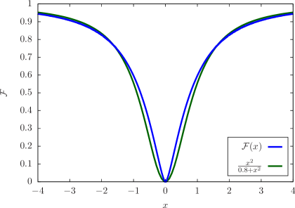
Figure 5: (Color online). Blue line: Magnetic field response, $\delta I_{t}(B)$, for the “parallel-antiparallel” blocking mechanism, is plotted from Eq. (54) in the units $1/\tau_{\scriptscriptstyle D}$ versus dimensionless magnetic field $B/B_{\scriptscriptstyle c}$. Green line: fit with conventional lineshape of OMAR, $x^{2}/(0.8+x^{2})$.

Our basic assumption is that the time, $\tau_{\scriptscriptstyle D}$, of formation and dissociation of a pair is much bigger than the recombination time, $\tau$. Only under this condition the pair will exercise the spin dynamics. Using the relation $\tau_{\scriptscriptstyle D}\gg\tau$, we can simplify the expression Eq. (44) for ${\overline{t}}$ of a typical pair

$$\overline{t}=\tau_{\scriptscriptstyle D}+\frac{\tau}{1-\left(\frac{\bm{\Omega}_{1}\cdot\bm{\Omega}_{2}}{|\bm{\Omega}_{1}||\bm{\Omega}_{2}|}\right)^{2}}.$$ (47)

We can also rewrite the current in the form $I=\frac{1}{\tau_{\scriptscriptstyle D}}-\delta I_{t}(B)$, where the field-dependent correction is defined as

$$\delta I_{t}(B)=\frac{\tau}{\tau_{\scriptscriptstyle D}^{2}}\frac{1}{1-\left(\frac{\bm{\Omega}_{1}\cdot\bm{\Omega}_{2}}{|\bm{\Omega}_{1}||\bm{\Omega}_{2}|}\right)^{2}+\frac{\tau}{\tau_{\scriptscriptstyle D}}}$$ (48)

As we will see below, the significant change of $\delta I_{t}$ with $B$ takes place in the domain where $B$ is much bigger than the hyperfine field. Therefore, we expand Eq. (48) with respect to $|{\bm{b}}_{\scriptscriptstyle e}|/B$ and $|{\bm{b}}_{\scriptscriptstyle h}|/B$. The principal ingredient of this step is the expansion of denominator

$$|\bm{\Omega}_{1}|^{2}|\bm{\Omega}_{2}|^{2}-(\bm{\Omega}_{1}\cdot\bm{\Omega}_{2})^{2}\\ \approx B^{2}\left[|\bm{b}_{\scriptscriptstyle e}-\bm{b}_{\scriptscriptstyle h}|^{2}-\left(\bm{b}_{\scriptscriptstyle e}\cdot\frac{\bm{B}}{B}-\bm{b}_{\scriptscriptstyle h}\cdot\frac{\bm{B}}{B}\right)^{2}\right].$$ (49)

Assuming identical Gaussian distributions of ${\bm{b}}_{\scriptscriptstyle e}$, ${\bm{b}}_{\scriptscriptstyle h}$

$$\mathcal{P}(\bm{b}_{i})=\frac{1}{(\pi b_{0})^{3/2}}\exp(-|\bm{b}_{i}|^{2}/b_{0}^{2}),$$ (50)

and choosing the $z$-direction along ${\bm{B}}$ we get

$$\langle\delta I_{t}(B)\rangle=\frac{B^{2}\tau}{\tau_{\scriptscriptstyle D}^{2}}\left<\frac{1}{(b_{1x}\!\!-\!b_{2x})^{2}+(b_{1y}\!\!-\!b_{2y})^{2}+\frac{\tau}{\tau_{\scriptscriptstyle D}}B^{2}}\right>.$$ (51)

The next step is averaging Eq. (51) over the remaining four components of the hyperfine fields. It is easiest to perform this integration by switching to $\bm{b}_{1}\pm\bm{b}_{2}$ and introducing the polar coordinates. The integrations over the sum and over the polar angle are elementary. The result can be cast in the form

$$\langle\delta I_{t}(B)\rangle=\frac{1}{\tau_{\scriptscriptstyle D}}\mathcal{F}\left(\frac{B}{B_{\scriptscriptstyle c}}\right),$$ (52)

where the characteristic field $B_{\scriptscriptstyle c}$ is given by

$$B_{\scriptscriptstyle c}=\left(\frac{2\tau_{\scriptscriptstyle D}}{\tau}\right)^{1/2}b_{0}.$$ (53)

The form of the function $\mathcal{F}$ is the following

$$\mathcal{F}(x)=2x^{2}\int\limits_{0}^{\infty}du\,\frac{u}{u^{2}+x^{2}}\,e^{-u^{2}}=x^{2}e^{x^{2}}\text{E}_{1}(x^{2}),$$ (54)

where $\text{E}_{1}(z)$ is the exponential integral function. From Eq. (53) we see that relation $\tau_{\scriptscriptstyle D}\gg\tau$ ensures that $B_{\scriptscriptstyle c}\gg b_{0}$, so that the expansion Eq. (49) of $\delta I_{t}(B)$ with respect to hyperfine fields is justified.

The magnetoresistance Eq. (52) is plotted in Fig. 5. We note that the shape, being a single-parameter function, $\mathcal{F}(x)$, can be very closely approximated with $x^{2}/(0.8+x^{2})$. This approximation, which is also plotted in Fig. 5, represents a standard fitting function for experimentally measured magnetoresistance. It can be seen that at $x\ll 1$ there is a small deviation of $\mathcal{F}(x)$ from the approximation. This is due to singular behavior of $\mathcal{F}(x)$ at small arguments. This singularity translates into the following behavior of $\delta I_{t}(B)$

$$\delta I_{t}(B)\underset{b_{0}<B<B_{\scriptscriptstyle c}}{\approx}\frac{\tau B^{2}}{2\tau_{\scriptscriptstyle D}^{2}\,b_{0}^{2}}\ln\left(\frac{2\tau_{\scriptscriptstyle D}\,b_{0}^{2}}{\tau B^{2}}\right).$$ (55)

On the physical level, the fact that the “body” of magnetoresistance lies in the domain $B\gg b_{0}$ suggests that the origin of the effect are trapping configurations for which ${\bm{\Omega}}_{1}$ and ${\bm{\Omega}}_{2}$ are almost parallel or antiparallel. In this regard, Eqs. (52) and (54) can be viewed as analytical, rather than numerical, as in Ref. Bobbert1, , treatment of the bipolaron mechanismBobbert1 .

V.2 Averaging in the soft-pair-dominant regime

Soft pairs are responsible for the second and third terms in the brackets of Eq. (45) for ${\overline{t}}$. The second term becomes big when the sum, ${\bm{\Omega}}_{1}+{\bm{\Omega}}_{2}$, becomes anomalously small. Still it cannot dominate over the contribution from the first term for the following reason. When ${\bm{\Omega}}_{1}+{\bm{\Omega}}_{2}$ is small, the expression in the parenthesis of the second term behaves as $({\bm{\Omega}}_{1}+{\bm{\Omega}}_{2})^{2}/|{\bm{\Omega}}_{1}|^{2}$. At the same time, for small ${\bm{\Omega}}_{1}-{\bm{\Omega}}_{2}$, the expression in the parenthesis of the first term behaves as $({\bm{\Omega}}_{1}-{\bm{\Omega}}_{2})^{2}/|{\bm{\Omega}}_{1}|^{2}$. In strong fields, the second expression is smaller than the first, leading to the larger $\delta I$, while in weak fields the two expressions give the same contribution to $\delta I$.

The third term in Eq. (45) captures the contribution of the slow modes to the current. Below we will study whether the averaging of this term over hyperfine fields can dominate over the “bipolaron” magnetic-field response given by Eq. (55).

Prior to performing averaging, we rewrite the current as $I=\frac{1}{\tau_{\scriptscriptstyle D}}-\delta I_{s}(B)$, like we did above. In the soft-pairs-dominated regime the expression for $\delta I_{s}(B)$ takes the form

$$\delta I_{s}(B)=\frac{1}{\tau_{\scriptscriptstyle D}}\left(\frac{1}{1+\frac{(|\bm{\Omega}_{1}|^{2}-|\bm{\Omega}_{2}|^{2})^{2}}{|\bm{\Omega}_{1}+\bm{\Omega}_{2}|^{2}}\tau\tau_{\scriptscriptstyle D}}\right).$$ (56)

For a typical configuration with $|{\bm{\Omega}}_{1}|\sim|{\bm{\Omega}}_{2}|$, the second term in denominator can be estimates as $|{\bm{\Omega}}_{1}|^{2}\tau\tau_{\scriptscriptstyle D}$, so that it is large in the slow-recombination regime. This is why the soft pairs with

$$(|{\bm{\Omega}}_{1}|-|{\bm{\Omega}}_{2}|)\sim\frac{1}{\sqrt{\tau\tau_{\scriptscriptstyle D}}}$$ (57)

give the major contribution to the average $\delta I_{s}(B)$. The latter fact allows one to simplify the averaging procedure. Namely, one can use the fact that for $\epsilon\ll 1$ the combination $\frac{\epsilon}{\epsilon^{2}+x^{2}}$ can be replaced by $\pi\delta(x)$. Thus, the expression to be averaged can be rewritten in the form

$$\delta I_{s}(B)=\frac{\pi}{\tau_{\scriptscriptstyle D}\sqrt{\tau\tau_{\scriptscriptstyle D}}}\delta\left(\frac{|\bm{\Omega}_{1}|^{2}-|\bm{\Omega}_{2}|^{2}}{|\bm{\Omega}_{1}+\bm{\Omega}_{2}|}\right).$$ (58)

The form Eq. (58) suggests that characteristic magnetic field determined from zero of the $\delta$-function is $B\sim b_{0}$, and yields the estimate $1/\tau^{1/2}\tau_{\scriptscriptstyle D}^{3/2}b_{0}$ for $\delta I_{s}(B)$. To compare the contribution of soft pairs to that of typical pairs this estimate should be compared to Eq. (55) taken at $B\sim b_{0}$. Soft pairs dominate if the condition

$$\sqrt{\frac{\tau_{\scriptscriptstyle D}}{\tau}}\gg b_{0}\tau$$ (59)

is met. Since $\tau_{\scriptscriptstyle D}$ is much bigger than $\tau$, this condition is compatible with the condition, $b_{0}\tau\gg 1$ necessary for slow recombination. Note in passing, that replacement of the denominator in Eq. (48) by a $\delta$-function, as we did for soft pairs, is not permissible. This follows, e.g., from Eq. (53) which suggests that the characteristic field $B_{\scriptscriptstyle c}$ is much bigger than $b_{0}$. Replacement of the denominator in Eq. (48) by a $\delta$-function would automatically fix the characteristic field at $B\sim b_{0}$.

In averaging of Eq. (58) over hyperfine configurations, we will assume from the outset that the characteristic hyperfine fields, $b_{1}$ and $b_{2}$, for the electron and hole are different, so that

$$\langle\delta I_{s}(B)\rangle=\frac{1}{\pi^{2}b_{1}^{3}b_{2}^{3}\sqrt{\tau\tau_{\scriptscriptstyle D}^{3}}}\int d^{3}\bm{b}_{\scriptscriptstyle e}\int d^{3}\bm{b}_{\scriptscriptstyle h}\\ \delta\left(\frac{|\bm{b}_{\scriptscriptstyle e}+\bm{B}|^{2}-|\bm{b}_{\scriptscriptstyle h}+\bm{B}|^{2}}{|\bm{b}_{\scriptscriptstyle e}+\bm{b}_{\scriptscriptstyle h}+2\bm{B}|^{2}}\right)\exp\left(-\frac{|\bm{b}_{\scriptscriptstyle e}|^{2}}{b_{1}^{2}}-\frac{|\bm{b}_{\scriptscriptstyle h}|^{2}}{b_{2}^{2}}\right).$$ (60)

Subsequent analysis will indicate that different $b_{1}$ and $b_{2}$ is a necessary condition for $\delta I_{s}$ to exhibit $B$-dependence.

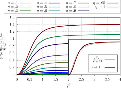
Figure 6: (Color online). Magnetic field response for the “soft-pair” mechanism is plotted from Eq. (66) versus magnetic field in the units of the hyperfine field $b_{1}$ for different values of the asymmetry parameter $\eta$. Inset: fit of the response in the limit of strong asymmetry with conventional lineshape of OMAR, $\sqrt{2}x^{2}/(0.23+x^{2})$.

The six-fold integral Eq. (60) can be reduced to a single integral in three steps. As a first step, we introduce new variables $\bm{v}=\bm{b}_{\scriptscriptstyle e}-\bm{b}_{\scriptscriptstyle h}$ and $\bm{u}=\bm{b}_{\scriptscriptstyle e}+\bm{b}_{\scriptscriptstyle h}+2\bm{B}$, so that Eq. (60) acquires the form

$$\langle\delta I_{s}(B)\rangle=\frac{1}{8\pi^{2}b_{1}^{3}b_{2}^{3}\sqrt{\tau\tau_{\scriptscriptstyle D}^{2}}}\int d^{3}\bm{u}\int d^{3}\bm{v}\;|\bm{u}|\,\delta(\bm{u}\cdot\bm{v})\\ \times\exp\left(-\alpha(\bm{u}-2\bm{B})^{2}+\beta(\bm{u}-2\bm{B})\cdot\bm{v}-\alpha|\bm{v}|^{2}\right),$$ (61)

with parameters $\alpha$ and $\beta$ defined as

$$\alpha=\frac{1}{4}\left(\frac{1}{b_{1}^{2}}+\frac{1}{b_{2}^{2}}\right),~{}~{}~{}\beta=\frac{1}{2}\left(\frac{1}{b_{1}^{2}}-\frac{1}{b_{2}^{2}}\right).$$ (62)

As a second step, we perform integration over the vector ${\bm{v}}$. The reason why this integration can be carried out analytically is that, upon choosing the $z$-direction along ${\bm{u}}$, the $\delta$-function fixes $v_{z}$ to be zero. The remaining two integrals over $v_{x}$ and $v_{y}$ are simply gaussian integrals, so we get

$$\langle\delta I_{s}(B)\rangle=\frac{1}{8\pi b_{1}^{3}b_{2}^{3}\alpha\sqrt{\tau\tau_{\scriptscriptstyle D}^{3}}}\int d^{3}\bm{u}\;\\ \exp\left[-\alpha(\bm{u}-2\bm{B})^{2}+\frac{\beta^{2}}{\alpha}\left(|\bm{B}|^{2}-\frac{(\bm{B}\cdot\bm{u})^{2}}{|\bm{u}|^{2}}\right)\right].$$ (63)

To perform the integration over ${\bm{u}}$, we switch to spherical coordinates with polar axis along ${\bm{B}}$. Then the integration over azimuthal angle reduces to multiplication by $2\pi$. The third step is the integration over the polar angle in Eq. (63). We have

$$\langle\delta I_{s}(B)\rangle=\frac{e^{-4\alpha\left(1-\frac{\beta^{2}}{4\alpha^{2}}\right)B^{2}}}{4b_{1}^{3}b_{2}^{3}\alpha\sqrt{\tau\tau_{\scriptscriptstyle D}^{3}}}\int\limits_{0}^{\infty}du\;u^{2}e^{-\alpha u^{2}}\\ \int\limits_{0}^{\pi}d\theta\sin\theta\exp\left(4\alpha uB\cos\theta-\frac{\beta^{2}}{\alpha}B^{2}\cos^{2}\theta\right).$$ (64)

Now we note that the integral over $\theta$ can be expressed via the error-functions in the following way

$$\int\limits_{-1}^{1}dx\,e^{-A^{2}x^{2}+Cx}=\frac{\sqrt{\pi}}{2A}e^{\frac{C^{2}}{4A^{2}}}\!\!\!\left[\text{erf}\left(\!\!A\!+\!\frac{C}{2A}\!\!\right)+\text{erf}\left(\!\!A\!-\!\frac{C}{2A}\!\!\right)\right].$$ (65)

We are left with a single integral over $u$, which can be cast in the form

$$\langle\delta I_{s}(B)\rangle=\frac{\sqrt{\pi}e^{-4\alpha\left(1-\frac{\beta^{2}}{4\alpha^{2}}\right)B^{2}}}{8b_{1}^{3}b_{2}^{3}\sqrt{\tau\tau_{\scriptscriptstyle D}^{3}}\sqrt{\alpha}\beta B}\int\limits_{0}^{\infty}du\;u^{2}\exp\left(-\alpha\left(1-\frac{4\alpha^{2}}{\beta^{2}}\right)u^{2}\right)\left[\text{erf}\left(\frac{\beta B}{\sqrt{\alpha}}+\frac{2\alpha^{3/2}u}{\beta}\right)+\text{erf}\left(\frac{\beta B}{\sqrt{\alpha}}-\frac{2\alpha^{3/2}u}{\beta}\right)\right].$$ (66)

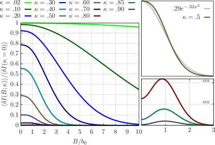
Figure 7: (Color online) Magnetic field response caused by the difference, in the $g$-factors of electron and hole is plotted from Eq. (73) for several values of relative difference, $\kappa$. Upper inset illustrates that the shape of the response is near-gaussian. Lower inset illustrates that at $\kappa$ close to $1$ the shape of the response develops a maximum.

V.3 Analysis of Eq. (66)

At this point we make an observation that for $b_{1}=b_{2}$, which is equivalent to $\beta=0$, magnetic field drops out of Eq. (66). The easiest way to see it is to set $\beta=0$ at the earlier stage of calculation, namely in Eq. (63)

$$\langle\delta I_{s}(b_{1}=b_{2})\rangle=\frac{1}{8\pi b_{1}^{3}b_{2}^{3}\alpha\sqrt{\tau\tau_{\scriptscriptstyle D}^{3}}}\int d^{3}\bm{u}\,e^{-\alpha(\bm{u}-2\bm{B})^{2}},$$ (67)

which is clearly independent of $\bm{B}$ after a simple coordinate shift. If we set $b_{1}=b_{2}$, then $\delta I_{s}$ is given by

$$\langle\delta I_{s}(b_{1}=b_{2})\rangle=\sqrt{\frac{\pi}{2\tau\tau_{\scriptscriptstyle D}^{3}}}\,\frac{1}{b_{1}},$$ (68)

in agreement with the qualitative estimate above.

Magnetic field dependence of $\langle\delta I_{s}\rangle$ emerges already at small values of asymmetry parameter defined as

$$\eta=1-\frac{b_{2}^{2}}{b_{1}^{2}}.$$ (69)

This is illustrated in Fig. 6, where $\langle\delta I_{s}(\eta,B)\rangle-\langle\delta I_{s}(\eta,0)\rangle$ in the units of $\langle\delta I_{s}(\eta=0)\rangle$, given by Eq. (68), is plotted for several values of $\eta$. We see that, as $\eta$ increases, the shape of the curves does not change much. For the saturation value the analysis of Eq. (66) yields

$$\frac{\langle\delta I_{s}(\eta,\infty)\rangle-\langle\delta I_{s}(\eta,0)\rangle}{\langle\delta I_{s}(\eta=0)\rangle}=\frac{\sqrt{2}\eta^{2}}{(2-\eta)^{5/2}}.$$ (70)

The result Eq. (66) can be recast in the more concise form in terms of the Dawson function $D(x)=e^{-x^{2}}\int\limits_{0}^{x}dt\,e^{t^{2}}$. The corresponding expression reads

$$\frac{\langle\delta I_{s}(\eta,B)\rangle}{\langle\delta I_{s}(0,0)\rangle}=\frac{\sqrt{2}}{\sqrt{2\!-\!\eta}}-\left(\!\frac{\eta}{2\!-\!\eta}\!\right)^{2}\frac{\sqrt{2}}{2z}D\left(\frac{2z}{\sqrt{2\!-\!\eta}}\right),$$ (71)

where we have introduced $z=B/b_{1}$.

In the limit of strong asymmetry, when $\eta$ is close to $1$, one gets a simple analytical expression for $\langle\delta I_{s}(B)\rangle$

$$\frac{\langle\delta I_{s}(\eta=1,B)\rangle}{\langle\delta I_{s}(\eta=0)\rangle}=\\ 2\left(\frac{B}{b_{1}}\right)^{2}\int\limits_{-1}^{1}dx\,\sqrt{1+x}\,\exp\left[-2\left(\frac{B}{b_{1}}\right)^{2}(1-x)\right].$$ (72)

At small $B$ the ratio Eq. (72) behaves quadratically, while at large $B$ it saturates as $\sqrt{2}\left(1-\frac{b_{1}^{2}}{8B^{2}}\right)$. Overall, similarly to $I_{t}(B)$, magnetoresistance Eq. (72) can be closely approximated with $\sqrt{2}x^{2}/(0.23+x^{2})$, as illustrated in Fig. 6.

V.4 Inequivalence of electron and hole $g$-factors

In the previous subsection we demonstrated that external magnetic field drops out from the general expression Eq. (60) when the variances $b_{1}$ and $b_{2}$ are equal. Here we note that averaging does not eliminate the $B$-dependence even when $b_{1}=b_{2}$, as long as the $g$-factors of the pair partners are different. Incorporating $g_{1}$ and $g_{2}$ into Eq. (60) is straightforward and amounts to multiplying ${\bm{b}}_{\scriptscriptstyle e}+{\bm{B}}$ by $1+\kappa$, while ${\bm{b}}_{\scriptscriptstyle h}+{\bm{B}}$ is multiplied by $1-\kappa$, where $\kappa$ is the relative difference in the $g$-factors. The three steps leading from Eq. (60) to Eq. (66) are exactly the same as for $\kappa=0$. Finite $\kappa$ modifies both the prefactor in the integral Eq. (66) and the arguments of the error functions in the integrand. It is convenient to analyze the magnetic field response by considering the ratio $\langle\delta I_{s}(B;\kappa)\rangle/\langle\delta I_{s}(\kappa=0)\rangle$, where the denominator is given by Eq. (68).

$$\frac{\langle\delta I_{s}(B;\kappa)\rangle}{\langle\delta I_{s}(\kappa=0)\rangle}=\frac{\exp\left(-\frac{2z^{2}}{1+\kappa^{2}}\right)}{2\sqrt{2}(1+\kappa^{2})\kappa z}\int\limits_{0}^{\infty}du\,u^{2}e^{-\zeta u^{2}}\left[\text{erf}\left(\frac{\kappa}{1-\kappa^{2}}(z+\gamma u)\right)+\text{erf}\left(\frac{\kappa}{1-\kappa^{2}}(z-\gamma u)\right)\right],$$ (73)

where $z=B/b_{1}$ is the scaled magnetic field. For notational convenience we introduced the $\kappa$-dependent terms $\zeta$ and $\gamma$, which are defined as

$$\zeta=\frac{1}{2(1-\kappa^{2})}\left(1+\frac{(1-\kappa^{2})^{3}}{2\kappa^{2}(1+\kappa^{2})^{2}}\right),$$ (74)

$$\gamma=\frac{1}{1-\kappa^{2}}\left(1+\frac{(1-\kappa^{2})^{3}}{\kappa^{2}(1+\kappa^{2})}\right).$$ (75)

It is seen that the arguments of the error-functions as well as the power in the exponent diverge in the limit $\kappa\rightarrow 1$, i.e. when the $g$-factor of one pair-partner is zero. This divergence signifies that magnetic field response is weak for small $(1-\kappa)$. The underlying reason for this is that the portion of soft pairs goes to zero if the levels of one of the partners are not split by a magnetic field. In Fig. 7 we plot the magnetic field response for different values of $\kappa$. There are two noteworthy features of this response. Firstly, the sign of response is opposite to that for inequivalent distributions of electrons and holes, see Fig. 6. Secondly, the shape of $\delta I_{s}(B)$ is not Lorentzian anymore. In fact, this shape is close to Gaussian, as illustrated in the inset. Another peculiar feature of $\delta I_{s}(B)$ which can be seen from Fig. 7 is that, for $\kappa$ close to $1$, the response $\delta I(B)$ develops a bump.

V.5 Averaging in the fast-recombination regime

Turning to Eq. (46) for $\overline{t}$ in the fast-recombination regime we notice that the second term in the square brackets has exactly the same form as the contribution of the soft pairs to $\overline{t}$ in the slow-recombination regime, see Eq. (45). The underlying reason is that, similarly to soft pairs, this second term also comes from the slow eigenmode. The origin of this slow eigenmode, i.e. orthogonalization of $S$-mode to all the other states, was discussed in detail in Sect. IIc. Since the configurational averaging for soft pairs was already carried out, we conclude that the magnetic field response in the fast-recombination regime is simply described by Eq. (66).

At this point we note that configurational averaging over slow pairs was based on the applicability of the condition $b_{0}^{2}\tau\tau_{\scriptscriptstyle D}\gg 1$. Therefore, it is important that this condition is compatible with fast-recombination, $b_{0}\tau\ll 1$, by virtue of a small parameter $\tau/\tau_{\scriptscriptstyle D}$.

In addition to the soft-pair contribution, Eq. (46) also contains a term with $|{\bm{\Omega}}_{1}\times{\bm{\Omega}}_{2}|^{2}$ in the denominator. This term becomes large when ${\bm{\Omega}}_{1}$ and ${\bm{\Omega}}_{2}$ are collinear. However, the statistical weight of these configurations is smaller than the statistical weight of the soft-pair contribution. Indeed, in order for the term with $|{\bm{\Omega}}_{1}\times{\bm{\Omega}}_{2}|^{2}$ in denominator to become large, the angle between the vectors ${\bm{\Omega}}_{1}$ and ${\bm{\Omega}}_{2}$ should be restricted to $\theta_{0}\sim 1/b_{0}\sqrt{\tau\tau_{\scriptscriptstyle D}}\ll 1$. In course of configurational averaging, the integral, $\int d\theta\sin\theta\ldots$, emerges which is small as $\theta_{0}^{2}$.

We now turn to the limit of very weak hyperfine fields for which the parameter $b_{0}^{2}\tau\tau_{\scriptscriptstyle D}$ is small. One may expect that magnetic field response is suppressed in this domain. What we demonstrate below is that this suppression is anomalously strong. Namely, the first term of the expansion of Eq. (46) with respect to $b_{0}^{2}\tau\tau_{\scriptscriptstyle D}$ does not contain the external field at all. This first term has the form

$$\overline{t}-2\tau_{\scriptscriptstyle D}=-\frac{\tau\tau_{\scriptscriptstyle D}^{2}}{16}\left[\frac{(|\bm{\Omega}_{1}|^{2}-|\bm{\Omega}_{2}|^{2})^{2}}{|\bm{\Omega}_{1}+\bm{\Omega}_{2}|^{2}}+\frac{4|\bm{\Omega}_{1}\times\bm{\Omega}_{2}|^{2}}{|\bm{\Omega}_{1}+\bm{\Omega}_{2}|^{2}}\right].$$ (76)

To realize that $B$ drops out of the expression in the square brackets it is convenient to first replace $|\bm{\Omega}_{1}\times\bm{\Omega}_{2}|^{2}$ by $|\bm{\Omega}_{1}|^{2}|\bm{\Omega}_{2}|^{2}-(\bm{\Omega}_{1}\cdot\bm{\Omega}_{2})^{2}$ and then use the identity

$$|\bm{\Omega}_{1}\!+\!\bm{\Omega}_{2}|^{2}|\bm{\Omega}_{1}\!-\!\bm{\Omega}_{2}|^{2}=(|\bm{\Omega}_{1}|^{2}+|\bm{\Omega}_{2}|^{2})^{2}-4(\bm{\Omega}_{1}\cdot\bm{\Omega}_{2})^{2}.$$ (77)

This leads to a drastic simplification of Eq. (76), which assumes the form

$$\overline{t}-2\tau_{\scriptscriptstyle D}=-\frac{\tau\tau_{\scriptscriptstyle D}^{2}}{16}|\bm{\Omega}_{1}-\bm{\Omega}_{2}|^{2}.$$ (78)

Since $|\bm{\Omega}_{1}-\bm{\Omega}_{2}|=|\bm{b}_{e}-\bm{b}_{h}|$, the magnetic field drops out of ${\overline{t}}$ in the first order in $\tau\tau_{\scriptscriptstyle D}b_{0}^{2}$.

VI Concluding remarks

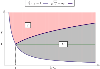
Figure 8: (Color online). Different domains on the plane $\left(b_{0}\tau_{\scriptscriptstyle D},~{}b_{0}\tau\right)$ illustrate the regions where different OMAR mechanisms dominate. The is no OMAR in the white domains. The pink domain corresponds to slow recombination, and OMAR is given by Eq. (52). In both the upper and the lower parts of the gray domain the OMAR is dominated by soft pairs and is described by Eq. (66). The green line divides the gray domain into subregions where the recombination is slow (upper part) and fast (lower part). The boundaries of the domains are: $b_{0}\tau=\frac{1}{b_{0}\tau_{\scriptscriptstyle D}}$, and $b_{0}\tau=(b_{0}\tau_{\scriptscriptstyle D})^{1/3}$.

1. Our findings can be summarized in the form of domains on the plane $\left(b_{0}\tau_{\scriptscriptstyle D},b_{0}\tau\right)$, as shown in Fig. 8. The fact that for small $b_{0}^{2}\tau\tau_{\scriptscriptstyle D}$ the OMAR response is absent is reflected in Fig. 8 by leaving the domain lying below the hyperbola uncolored. Large hyperfine fields, $b_{0}\tau>1$, correspond to slow recombination. As we have demonstrated above, the OMAR for $b_{0}\tau>1$ can be dominated either by “typical” pairs or by “soft” pairs. The corresponding regions, $I$ and $II$, are colored in Fig. 8 by pink and gray, respectively. The domains are separated by the curve $b_{0}\tau=(b_{0}\tau_{\scriptscriptstyle D})^{1/3}$. Eq. (52) describes OMAR in the domain $I$, while in the domain $II$ Eq. (66) applies. Note that in the domain $II$ only the part above the green line corresponds to slow recombination. The part below the green line corresponds to fast recombination, but Eq. (66) applies in both domains. The diagram describes the regimes of OMAR in low applied fields, $B\sim b_{0}$. As $B$ increases above $b_{0}$, the gray domain shrinks.

2. The OMAR response from the soft pairs relies exclusively on the asymmetry between electron and hole. The evidence in favor of such an asymmetry was inferred in Ref. E-H, from the analysis of magnetic-resonance data in organic devices. In Ref. E-H, , the ratio $b_{2}/b_{1}$ was estimated to be close to $3$, which leads to the value of the asymmetry parameter $\eta\approx 0.9$. Note, that bipolaron mechanism is insensitive to the asymmetry between electron and hole.

3. “Parallel-antiparallel” mechanism of Ref. Bobbert1, yields the OMAR response on the level of rate equations with the transition rates calculated from the golden rule. The applicability of this treatment requires that the separation of Zeeman levels is large compared to their widths. On the other hand, the OMAR response based on soft pairs, studied in the present paper, comes entirely from pairs for which the Zeeman levels are almost aligned. This requires one to go beyond the golden rule. Previously, a similar situation was encounteredsubradiance2 by M. Schultz and F. von Oppen in the study of transport through a nanostructure with almost degenerate levels. The role of spin-selective recombination was played by coupling to the leads which was strongly different for symmetric and antisymmetric combinations of the wave functions. M. Schultz and F. von Oppen pointed out that when two levels are closer in energy than the width of each of them, then the conventional rate-equation-based description is insufficient.

   On the physical level, the near-degeneracy implies that some spin configuration is preserved during many precession periods, i.e. the dynamics is important. To account for dynamics, it is intuitively appealing to take the result of Schulten and Wolynes, Eqs. (2)-(3) , and multiply it by a factor describing exponential decay of population of states due to recombination. Such an approach was adopted in Ref. Flatte1, . What this approach misses is the feedback of recombination on the pair dynamics. It is the central message of the present paper that this effect is strong in certain regimes, since feedback creates long-living modes.

4. The “parallel-antiparallel” mechanism of Ref. Bobbert1, is based on the picture of incoherent hopping of one of the charge carriers on the site already occupied by the other carrier. We considered the transport model applicable for bipolar system where the passage of current is due to recombination of electrons and holes. However, the principal ingredients of both models are the same: (a) in both transport models the spins of the carriers precess in their effective magnetic fields, the precession being governed by the same Hamiltonian Eq. (1); (b) the passage of current is the sequence of cycles, only one step of each cycle is sensitive to the spin precession; (c) whether it is a hop or recombination, it occurs only from the $S$-spin configuration; (d) if either the hop or recombination act takes too long, the carriers bypass each other.

5. Both the “parallel-antiparallel” pairs and soft pairs create the OMAR response by blocking the current. The origin of this blocking is completely different for the two mechanisms. In the former, the current is blocked due to collinearity of full fields for the pair-partners, while for the latter the blocking is due to coincidence of their absolute values. In general, both contributions are present in the fast-recombination regime. The contribution of soft pairs in this regime dominates by virtue of their statistical weight.

6. Another distinctive feature of the soft-pairs mechanism follows from Eq. (56). It contains a combination $(|\bm{\Omega}_{1}|^{2}-|\bm{\Omega}_{2}|^{2})^{2}$ in the denominator. As the precession frequencies change with external field, ${\bm{B}}$, the pair undergoes evolution from typical to soft (when $|{\bm{\Omega}}_{1}|=|{\bm{\Omega}}_{2}|$) and back to typical. Importantly, this evolution takes place within a narrow interval of ${\bm{B}}$, so that at a given ${\bm{B}}$ only certain sparse pairs contribute to the current. As demonstrated in Ref. mesoscopics, , this redistribution of soft pairs gives rise to mesoscopic features in $I(B)$ in small samples.

7. We have demonstrated above that regardless of whether the OMAR is due to blocking caused by “parallel-antiparallel” configurations, as in Ref. Bobbert1, , or due to soft pairs, the shape of the response is always close to $B^{2}/(B^{2}+B_{\scriptscriptstyle c}^{2})$. This result was obtained under the assumption that $\tau$ and $\tau_{\scriptscriptstyle D}$ are fixed. If the values of $\tau$ and $\tau_{\scriptscriptstyle D}$ are broadly distributed, then the adequate description of transport should be based on the percolative approachFlatte1 . However, within our minimal model, the current is the sum of partial currents through the chains, see Fig. 3. Then, with wide spread in cycle durations, $\overline{t}$, the current will be limited by pairs with longest $\overline{t}$ present in each chain.

Appendix A Time Evolution and the Schrodinger Equation

In this Appendix we sketch a formal derivation of Eqs. (19) and (37) starting from the Liouville equation for the density operator, $\widehat{\sigma}$,

$$\frac{\partial\widehat{\sigma}}{\partial t}=-i[\widehat{\mathcal{H}},\widehat{\sigma}]+\widehat{L}(\widehat{\sigma}),$$ (79)

where the term $\widehat{L}(\widehat{\sigma})$ describes relaxation, which in our case is recombination from $S$ to the ground state, $G$. The ground state with energy $-\mathcal{E}$ is included into the bare Hamiltonian

$$\widehat{\mathcal{H}} =\widehat{H}+\widehat{H}_{G}$$ (80)

$$=\left(\widehat{\bm{S}}_{1}\cdot\bm{B}_{1}+\widehat{\bm{S}}_{2}\cdot\bm{B}_{2}\right)-\mathcal{E}\left|{G}\right>\left<{G}\right|.$$ (81)

Then the operator $\widehat{L}(\widehat{\sigma})$ cast into conventional Lindblad formLindblad reads

$$\widehat{L}(\widehat{\sigma})=\frac{1}{2}\Gamma\left(2\left|{G}\right>\left<{S}\right|\widehat{\sigma}\left|{S}\right>\left<{G}\right|-\widehat{\sigma}\left|{S}\right>\left<{S}\right|-\left|{S}\right>\left<{S}\right|\widehat{\sigma}\right),$$ (82)

where $\frac{1}{2}\Gamma=\tau^{-1}$ is the inverse recombination time.

Denote with $i$, $k$ different spin configurations of the pair prior to recombination. The form Eq. (82) of the dissipation ensures independence of the elements of the density matrix with subindices $i$, $k$ from the elements containing subindex ${\scriptscriptstyle G}$. This decoupling follows from the full system of the equations of motion

$$\frac{\partial\sigma_{\scriptscriptstyle GG}}{\partial t} =\Gamma\sigma_{\scriptscriptstyle SS},$$ (83)

$$\frac{\partial\sigma_{\scriptscriptstyle Gk}}{\partial t} =-\mathcal{E}\sigma_{\scriptscriptstyle Gk}-\sum_{i}\sigma_{\scriptscriptstyle Gi}\mathcal{H}_{\scriptscriptstyle ik}-\frac{1}{2}\Gamma\sigma_{\scriptscriptstyle Gk}\delta_{\scriptscriptstyle Sk},$$ (84)

$$\frac{\partial\sigma_{\scriptscriptstyle ik}}{\partial t} =-i[\widehat{\mathcal{H}},\widehat{\sigma}]_{\scriptscriptstyle ik}-\frac{1}{2}\Gamma\left\{\widehat{\sigma},\left|{S}\right>\left<{S}\right|\right\}_{\scriptscriptstyle ik}.$$ (85)

Eq. (85) couples only the elements of $4\times 4$ matrix, which we denote with $\rho$, so that Eq. (85) represents equation of motion for $\rho$. These equations can be rewritten in the form similar to Eq. (79)

$$\frac{\partial\widehat{\rho}}{\partial t}=-i[\widehat{H},\widehat{\rho}]+\widehat{L}(\widehat{\rho}),$$ (86)

with dissipation term redefined as $\widehat{L}(\widehat{\rho})=-\frac{1}{2}\Gamma\left\{\widehat{\rho},\left|{S}\right>\left<{S}\right|\right\}$. To derive Eq. (19), we search for solution of Eq. (86) in the form

$$\rho(t)=\left|{\psi(t)}\right>\left<{\psi(t)}\right|,$$ (87)

and find that $\psi(t)$ must satisfy the following non-hermitian Schrödinger equation

$$i\frac{\partial}{\partial t}\left|{\psi(t)}\right>=\widehat{H}^{\prime}\left|{\psi(t)}\right>,$$ (88)

where $\widehat{H}^{\prime}$ is defined as $\widehat{H}^{\prime}=\widehat{H}-i\frac{\Gamma}{2}\left|{S}\right>\left<{S}\right|$. The fact that decoupling Eq. (87) is valid follows from a straightforward calculation

$$i\frac{\partial}{\partial t}\left|{\psi}\right>\left<{\psi}\right| =\left(i\frac{\partial}{\partial t}\left|{\psi}\right>\right)\left<{\psi}\right|+\left|{\psi}\right>\left(i\frac{\partial}{\partial t}\left<{\psi}\right|\right)$$ (89)

$$=H^{\prime}\left|{\psi}\right>\left<{\psi}\right|-\left|{\psi}\right>\left<{\psi}\right|(H^{\prime})^{\dagger}$$ (90)

$$=\left(H-i\frac{\Gamma}{2}\left|{S}\right>\left<{S}\right|\right)\left|{\psi}\right>\left<{\psi}\right|$$

$$\quad\quad-\left|{\psi}\right>\left<{\psi}\right|\left(H+i\frac{\Gamma}{2}\left|{S}\right>\left<{S}\right|\right)$$ (91)

$$=[H,\left|{\psi}\right>\left<{\psi}\right|]-i\frac{\Gamma}{2}\left\{\left|{S}\right>\left<{S}\right|,\left|{\psi}\right>\left<{\psi}\right|\right\}.$$ (92)

Now Eq. (19) immediately emerges as an equation for eigenvalues of the operator $\widehat{H}^{\prime}$.

Appendix B Derivation of Eq. (37)

To derive Eq. (37) for recombination time from random initial state, we first find the expression for recombination time, $t_{\psi_{0}}$, from a given initial state, $\psi_{0}$, in terms of the solution of Eq. (86) for $\rho(t)$ complemented with condition $\rho(0)=\left|{\psi_{0}}\right>\left<{\psi_{0}}\right|$. The expression for $t_{\psi_{0}}$ in terms of the full density matrix $\widehat{\sigma}(t)$ reads

$$t_{\psi_{0}}=\int_{0}^{\infty}\left(dt\,\frac{\partial\sigma_{\scriptscriptstyle GG}}{\partial t}\right)t.$$ (93)

The meaning of the expression in the brackets is the probability that recombination took place between $t$ and $t+dt$. The expression for $t_{\psi_{0}}$ in terms of $\rho(t)$ follows from the relation

$$\sigma_{\scriptscriptstyle GG}+\text{Tr}\,\rho=1.$$ (94)

Performing integration by parts, we obtain

$$t_{\psi_{0}}=\int_{0}^{\infty}\!\!\!\!dt\,\text{Tr}\,\rho(t).$$ (95)

To find the recombination time $\langle t_{\scriptscriptstyle R}\rangle$ from the random initial state the time $t_{\psi_{0}}$ should be averaged over initial states. One way to perform this averaging is to fix a certain orthonormal basis, $\Phi_{k}$, expand $\psi_{0}$ as

$$\psi_{0}=\sum_{k}c_{k}\Phi_{k},$$ (96)

and express $t_{\psi_{0}}$ as bilinear form in $c_{k}$. This yields

$$t_{\psi_{0}} =\int_{0}^{\infty}\!\!\!\!dt\,\text{Tr}\left[\widehat{U}(t)\psi_{0}^{\ast}\psi_{0}\widehat{U}^{\dagger}(t)\right]$$ (97)

$$=\int_{0}^{\infty}\!\!\!\!dt\,\text{Tr}\left[\widehat{U}(t)\left[\sum_{k}c_{k}\Phi_{k}\right]\left[\sum_{k^{\prime}}{c_{k^{\prime}}}^{\!\!\!\!*}{\Phi_{k^{\prime}}}^{\!\!\!\!\!*}\,\right]\widehat{U}^{\dagger}(t)\right]$$ (98)

$$=\sum_{k,k^{\prime}}c_{k}{c_{k^{\prime}}}^{\!\!\!\!*}\int_{0}^{\infty}\!\!\!\!dt\,\text{Tr}\left[\widehat{U}(t)\Phi_{k}{\Phi_{k^{\prime}}}^{\!\!\!\!\!*}\,\widehat{U}^{\dagger}(t)\right],$$ (99)

where $\widehat{U}(t)$ is the non-unitary evolution operator. Now the averaging over initial conditions reduces to averaging over $c_{k}$ according to the rule $\langle c_{k}{c_{k^{\prime}}}^{\!\!\!\!*}\rangle=\frac{1}{4}\delta_{k,k^{\prime}}$. This averaging is straightforward leading to

$$\langle t_{\scriptscriptstyle R}\rangle =\frac{1}{4}\sum_{k}\int_{0}^{\infty}\!\!\!\!dt\,\text{Tr}\left[\widehat{U}(t)\Phi_{k}{\Phi_{k}}^{\!\!\!\!*}\,\widehat{U}^{\dagger}(t)\right]$$ (100)

The remaining task is to express the sum, Eq. (100), in terms of eigenvalues and eigenvectors of a non-hermitian Schrödinger equation, Eq. (88). To accomplish this task we will use the expansion of the solutions $\psi_{\scriptscriptstyle k}$ of Eq. (88), which we, for brevity, denote with $\left|{\lambda_{\scriptscriptstyle k}}\right>$, in terms of the orthonormal basis $\Phi_{\scriptscriptstyle k}$, which we denote with $\left|{k}\right>$.

In terms of these new notations Eq. (88) and the time evolution operator can be written as

$$\widehat{H}^{\prime}\left|{\lambda_{j}}\right>=\lambda_{j}\left|{\lambda_{j}}\right>,\quad\widehat{U}(t)\left|{\lambda_{j}}\right>=e^{-i\lambda_{j}t}\left|{\lambda_{j}}\right>.$$ (101)

It is also convenient to introduce a matrix, $\widehat{d}$, which relates the elements of the basis to the solutions of Eq. (88). Namely,

$$\left|{k}\right>=\sum_{l}d_{kl}\left|{\lambda_{l}}\right>.$$ (102)

Substituting Eq. (102) into Eq. (101), we find

$$\widehat{U}(t)\left|{k}\right>=\sum_{l}d_{kl}\widehat{U}(t)\left|{\lambda_{l}}\right>=\sum_{l}d_{kl}e^{-i\lambda_{l}t}\left|{\lambda_{l}}\right>.$$ (103)

Next we introduce, $\widehat{g}$, which is the matrix of scalar products

$$g_{ij}=\left<\left.{\lambda_{i}}\right|{\lambda_{j}}\right>.$$ (104)

Using the definitions Eq. (102) and Eq. (104) we express $\langle t_{\scriptscriptstyle R}\rangle$, defined by Eq. (100), in terms of the matrices $\widehat{d}$ and $\widehat{g}$

$$\langle t_{\scriptscriptstyle R}\rangle =\frac{1}{4}\sum_{k}\int\limits_{0}^{\infty}dt\,\text{Tr}\left[\widehat{U}(t)\left|{k}\right>\left<{k}\right|\widehat{U}^{\dagger}(t)\right],$$ (105)

$$=\frac{1}{4}\sum_{k}\int_{0}^{\infty}dt\,\text{Tr}\left[\widehat{U}\left(\sum_{l}d_{kl}\left|{\lambda_{l}}\right>\right)\right.$$

$$\quad\quad\quad\quad\quad\quad\quad\quad\left.\times\left(\sum_{m}d_{km}^{\ast}\left<{\lambda_{m}}\right|\right)\widehat{U}^{\dagger}\right],$$ (106)

$$=\frac{1}{4}\sum_{klm}\int\limits_{0}^{\infty}dt\,e^{-i(\lambda_{l}-\lambda_{m}^{\ast})t}d_{kl}d_{km}^{\ast}\text{Tr}\left[\left|{\lambda_{l}}\right>\left<{\lambda_{m}}\right|\right],$$ (107)

$$=\frac{1}{4}\sum_{lm}\frac{1}{i(\lambda_{l}-\lambda_{m}^{\ast})}g_{ml}\left(\sum_{k}d_{kl}d_{km}^{\ast}\right).$$ (108)

In the last identity we have isolated the combination of the elements of the matrix $\widehat{d}$. The reason is that this combination can be cast in the form

$$\sum_{k}d_{kl}d_{km}^{\ast}=g^{-1\ast}_{ml}.$$ (109)

To prove the latter identity, we start from the matrix relation

$$\left<\left.{\lambda_{l}}\right|{i}\right>=\sum_{j}d_{ij}\left<\left.{\lambda_{l}}\right|{\lambda_{j}}\right>=\sum_{j}d_{ij}g_{lj},$$ (110)

and invert it to obtain

$$d_{ij}=\sum_{l}g_{jl}^{-1}\left<\left.{\lambda_{l}}\right|{i}\right>.$$ (111)

Next we complex conjugate both sides of Eq. (111) which yields

$$d_{ij}^{\ast}=\sum_{l}g_{jl}^{-1\ast}\left<\left.{\lambda_{l}}\right|{i}\right>^{\ast}=\sum_{l}g_{jl}^{-1\ast}\left<\left.{i}\right|{\lambda_{l}}\right>.$$ (112)

Now, the identity Eq. (109) emerges as a result of straight-forward calculation

$$\sum_{k}d_{kl}d_{km}^{\ast} =\sum_{k}\left(\sum_{j}g^{-1}_{lj}\left<\left.{\lambda_{j}}\right|{k}\right>\right)\left(\sum_{n}g^{-1\ast}_{mn}\left<\left.{k}\right|{\lambda_{n}}\right>\right),$$ (113)

$$=\sum_{jk}g^{-1}_{lj}g^{-1\ast}_{mn}\left<{\lambda_{j}}\right|\left(\sum_{k}\left|{k}\right>\left<{k}\right|\right)\left|{\lambda_{n}}\right>$$ (114)

$$=\sum_{jn}g^{-1}_{lj}g^{-1\ast}_{mn}g_{jn}$$ (115)

$$=g^{-1\ast}_{ml}.$$ (116)

Finally, substituting Eq. (109) into Eq. (108), we arrive at Eq. (37) of the main text.

References

- (1) E. L. Frankevich, I. A. Sokolik, D. I. Kadyrov, and V. M. Kobryanskii, Pis’ma Zh. Eksp. Teor. Fiz. 36, 401 (1982) [JETP Lett. 36, 488 (1982)].
- (2) E. L. Frankevich, A. A. Lymarev, I. Sokolik, F. E. Karasz, S. Blumstengel, R. H. Baughman, and H. H. Hörhold, Phys. Rev. B 46, 9320 (1992).
- (3) K. M. Salikhov, Y. N. Molin, R. Z. Sagdeev, and A. L. Buchachenko, in Spin Polarization and Magnetic Effects in Radical Reactions, edited by Y. N. Molin (Elsevier, Amsterdam, 1984), pp. 32-116, and the review U. E. Steiner and T. Ulrich, Chem. Rev. 89, 51 (1989).
- (4) K. Schulten and P. G. Wolynes, J. Chem. Phys. 68, 3292 (1978).
- (5) T. L. Francis, Ö. Mermer, G. Veeraraghavan, and M. Wohlgenannt, New J. Phys. 6, 185 (2004).
- (6) Ö. Mermer, G. Veeraraghavan, T. L. Francis, Y. Sheng, D. T. Nguyen, M. Wohlgenannt, A. Köhler, M. K. Al-Suti, and M. S. Khan, Phys. Rev. B 72, 205202 (2005).
- (7) Y. Sheng, T. D. Nguyen, G. Veeraraghavan, O. Mermer, M. Wohlgenannt, S. Qiu, and U. Scherf, Phys. Rev. B 74, 045213 (2006).
- (8) F. Wang, F. Maciá, M. Wohlgenannt, A. D. Kent, and M. E. Flatté, Phys. Rev. X 2, 021013 (2012).
- (9) P. Desai, P. Shakya, T. Kreouzis, and W. P. Gillin, Phys. Rev. B 76, 235202 (2007); Sijie Zhang, N. J. Rolfe, P. Desai, P. Shakya, A. J. Drew, T. Kreouzis, and W. P. Gillin, Phys. Rev. B 86, 075206 (2012).
- (10) F. J. Wang, H. Bässler, and Z. Valy Vardeny, Phys. Rev. Lett. 101, 236805 (2008).
- (11) T. D. Nguyen, G. Hukic-Markosian, F. Wang, L. Wojcik, X.-G. Li, E. Ehrenfreund, and Z. V. Vardeny, Nat. Mater. 9, 345 (2010).
- (12) T. D. Nguyen, B. R. Gautam, E. Ehrenfreund, and Z. V. Vardeny, Phys. Rev. Lett. 105, 166804 (2010).
- (13) Tho D. Nguyen, T. P. Basel, Y.-J. Pu, X-G. Li, E. Ehrenfreund, and Z. V. Vardeny, Phys. Rev. B 85, 245437 (2012).
- (14) F. L. Bloom, W. Wagemans, M. Kemerink, and B. Koopmans, Phys. Rev. Lett. 99, 257201 (2007).
- (15) P. A. Bobbert, T. D. Nguyen, F. W. A. van Oost, B. Koopmans, and M. Wohlgenannt, Phys. Rev. Lett. 99, 216801 (2007).
- (16) W. Wagemans, F. L. Bloom, P. A. Bobbert, M. Wohlgenannt, and B. Koopmans, J. Appl. Phys. 103, 07F303 (2008).
- (17) F. L. Bloom, M. Kemerink, W. Wagemans, and B. Koopmans, Phys. Rev. Lett. 103, 066601 (2009).
- (18) S. P. Kersten, A. J. Schellekens, B. Koopmans, and P. A. Bobbert, Phys. Rev. Lett. 106, 197402 (2011).
- (19) W. Wagemans, A. J. Schellekens, M. Kemper, F. L. Bloom, P. A. Bobbert, and B. Koopmans Phys. Rev. Lett. 106, 196802 (2011).
- (20) W. Wagemans and B. Koopmans, Phys. Status Solidi B 248, 1029 (2011).
- (21) V. N. Prigodin, J. D. Bergeson, D. M. Lincoln, and A. J. Epstein, Synth. Met. 156, 757 (2006).
- (22) N. J. Harmon and M. E. Flatté, Phys. Rev. Lett. 108, 186602 (2012); Phys. Rev. B 85, 075204 (2012); Rev. B 85, 245213 (2012).
- (23) R. H. Dicke, Phys. Rev. 93, 99 (1954).
- (24) T. V. Shahbazyan and M. E. Raikh, Phys. Rev. B 49, 17123 (1994).
- (25) M. G. Schultz and F. von Oppen, Phys. Rev. B 80, 033302 (2009).
- (26) J. König, Y. Gefen, and G. Schön, Phys. Rev. Lett. 81, 4468 (1998).
- (27) D. R. McCamey, K. J. van Schooten, W. J. Baker, S.-Y. Lee, S.-Y. Paik, J. M. Lupton, and C. Boehme, Phys. Rev. Lett. 104, 017601 (2010); S.-Y. Lee, S.-Y. Paik, D. R. McCamey, J. Yu, P. L. Burn, J. M. Lupton, and C. Boehme, J. Am. Chem. Soc. 133, 072019 (2011).
- (28) R. C. Roundy, Z. V. Vardeny, M. E. Raikh, e-print arXiv:1210.3443v1 (2012).
- (29) G. Lindblad, Commun. Math. Phys. 48, 119 (1976).