Performance Analysis of Heterogeneous Feedback Design in an OFDMA Downlink
with Partial and Imperfect Feedback

Abstract

Current OFDMA systems group resource blocks into subband to form the basic feedback unit. Homogeneous feedback design with a common subband size is not aware of the heterogeneous channel statistics among users. Under a general correlated channel model, we demonstrate the gain of matching the subband size to the underlying channel statistics motivating heterogeneous feedback design with different subband sizes and feedback resources across clusters of users. Employing the best-M partial feedback strategy, users with smaller subband size would convey more partial feedback to match the frequency selectivity. In order to develop an analytical framework to investigate the impact of partial feedback and potential imperfections, we leverage the multi-cluster subband fading model. The perfect feedback scenario is thoroughly analyzed, and the closed form expression for the average sum rate is derived for the heterogeneous partial feedback system. We proceed to examine the effect of imperfections due to channel estimation error and feedback delay, which leads to additional consideration of system outage. Two transmission strategies: the fix rate and the variable rate, are considered for the outage analysis. We also investigate how to adapt to the imperfections in order to maximize the average goodput under heterogeneous partial feedback.

I Introduction

Leveraging feedback to obtain the channel state information at the transmitter (CSIT) enables a wireless system to adapt its transmission strategy to the varying wireless environment. The growing number of wireless users, as well as their increasing demands for higher data rate services impose a significant burden on the feedback link. In particular for OFDMA systems, which have emerged as the core technology in 4G and future wireless systems, full CSIT feedback may become prohibitive because of the large number of resource blocks. This motivates more efficient feedback design approaches in order to achieve performance comparable to a full CSIT system with reduced feedback. In the recent years, considerable work and effort has been focused on limited or partial feedback design, e.g., see [1] and the references therein. To the best of our knowledge, most of the existing partial feedback designs are homogeneous, i.e., users’ feedback consumptions do not adapt to the underlying channel statistics. In this paper, we propose and analyze a heterogeneous feedback design, which aligns users’ feedback needs to the statistical properties of their wireless environments.

Current homogeneous feedback design in OFDMA systems groups the resource blocks into subband [2] which forms the basic scheduling and feedback unit. Since the subband granularity is determined by the frequency selectivity, or the coherence bandwidth of the underlying channel, it would be beneficial to adjust the subband size of different users according to their channel statistics. Empirical measurements and analysis from the channel modeling field have shown that the root mean square (RMS) delay spread which is closely related to the coherence bandwidth, is both location and environment dependent [3, 4]. The typical RMS delay spread for an indoor environment in WLAN does not exceed hundreds of nanoseconds; whereas in the outdoor environment of a cellular system, it can be up to several microseconds. Intuitively, users with lower RMS delay spread could model their channel with a larger subband size and require less feedback resource than the users with higher RMS delay spread. Herein, we investigate this heterogeneous feedback design in a multiuser opportunistic scheduling framework where the system favors the user with the best channel condition to exploit multiuser diversity [5, 6]. There are two major existing partial feedback strategies for opportunistic scheduling, one is based on thresholding where each user provides one bit of feedback per subband to indicate whether or not the particular channel gain exceeds a predetermined or optimized threshold [7, 8, 9, 10]. The other promising strategy currently considered in practical systems such as LTE [11] is the best-M strategy, where the receivers order and convey the M best channels [12, 13, 14, 15, 16, 17, 18, 19]. The best-M partial feedback strategy is embedded in the proposed heterogeneous feedback framework. Apart from the requirement of partial feedback to save feedback resource, the study of imperfections is also important to understand the effect of channel estimation error and feedback delay on the heterogeneous feedback framework. These imperfections are also considered in our work.

I-A Focus and Contributions of the Paper

An important step towards heterogeneous feedback design is leveraging the “match” among coherence bandwidth, subband size and partial feedback. Under a given amount of partial feedback, if the subband size is much larger than the coherence bandwidth, then multiple independent channels could exist within a subband and the subband-based feedback could only be a coarse representative of the channels. On the other hand, if the subband size is much smaller than the coherence bandwidth, then channels in adjacent subbands are likely to be highly correlated and requiring feedback on adjacent subbands could be a waste of resource; or a small amount of subband-based partial feedback may not be enough to reflect the channel quality. In order to support this heterogeneous framework, we first consider the scenario of a general correlated channel model with one cluster of users with the same coherence bandwidth. The subband size is adjustable and each user employs the best-M partial feedback strategy to convey the M best channel quality information (CQI) which is defined to be the subband average rate. The simulation result shows that a suitable chosen subband size yields higher average sum rate under partial feedback conforming the aforementioned intuition. This motivates the design of heterogeneous feedback to “match” the subband size to the coherence bandwidth. The above-mentioned study, though closely reflects the relevant mechanism, is not analytically tractable due to two main reasons. Firstly, the general correlated channel model complicates the statistical analysis of the CQI. Secondly, the use of subband average rate as CQI makes it difficult to analyze the multi-cluster scenario. Therefore, a simplified generic channel model is needed that balances the competing needs of analytical tractability and practical relevance.

In order to facilitate analysis, a subband fading channel model is developed that generalizes the widely used frequency domain block fading channel model. The subband fading model is suited for the multi-cluster analysis. According to the subband fading model, the channel frequency selectivity is flat within each subband, and independent across subbands. Since the subband sizes are different across different clusters, the number of independent channels are heterogeneous across clusters and this yields heterogeneous partial feedback design. Another benefit of the subband fading model is that the CQI becomes the channel gain and thus facilitate further statistical analysis. Under the multi-cluster subband fading model and the assumption of perfect feedback, we derive a closed form expression for the average sum rate. Additionally, we approximate the sum rate ratio for heterogeneous design, i.e., the ratio of the average sum rate obtained by a partial feedback scheme to that achieved by a full feedback scheme, in order to choose different best-M for users with different coherence bandwidth. We also compare and demonstrate the potential of the proposed heterogeneous feedback design against the homogeneous case under the same feedback constraint in our simulation study.

The average sum rate helps in understanding the system performance with perfect feedback. In practical feedback systems, imperfections occur such as channel estimation error and feedback delay. These inevitable factors degrade the system performance by causing outage [21, 22]. Therefore, rather than using average sum rate as the performance metric, we employ the notion of average goodput [23, 24, 25] to incorporate outage probability. Under the multi-cluster subband fading model, we perform analysis on the average goodput and the average outage probability with heterogeneous partial feedback. In addition to examining the impact of imperfect feedback on multiuser diversity [26, 27], we also investigate how to adapt and optimize the average goodput in the presence of these imperfections. We consider both the fixed rate and the variable rate scenarios, and utilize bounding technique and an efficient approximation to derive near-optimal strategies.

To summarize, the contributions of this paper are threefold: a conceptual heterogeneous feedback design framework to adapt feedback amount to the underlying channel statistics, a thorough analysis of both perfect and imperfect feedback systems under the multi-cluster subband fading model, and the development of approximations and near-optimal approaches to adapt and optimize the system performance. The rest of the paper is organized as follows. The motivation under the general correlated channel model and the development of system model is presented in Section II. Section III deals with perfect feedback, and Section IV examines imperfect feedback due to channel estimation error and feedback delay. Numerical results are presented in Section V. Finally, Section VI concludes the paper.

II System Model

II-A Motivation for Heterogeneous Partial Feedback

This part provides justification for the adaptation of subband size with one cluster of users under the general correlated channel model, and motivates the design of heterogeneous partial feedback for the multi-cluster scenario in Section II-B. Consider a downlink multiuser OFDMA system with one base station and $K$ users. One cluster of user is assumed in this part and users in this cluster are assumed to experience the same frequency selectivity. The system consists of $N_{\mathsf{c}}$ subcarriers. $H_{k,n}$, the frequency domain channel transfer function between transmitter and user $k$ at subcarrier $n$, can be written as:

$$H_{k,n}=\sum_{l=0}^{L-1}\sigma_{l}F_{k,l}\exp\left(-\frac{j2\pi ln}{N_{\mathsf{c}}}\right),$$ (1)

where $L$ is the number of channel taps, $\sigma_{l}$ for $l=0,\ldots,L-1$ represents the channel power delay profile and is normalized, i.e., $\sum_{l=0}^{L-1}\sigma_{l}^{2}=1$, $F_{k,l}$ denotes the discrete time channel impulse response, which is modeled as complex Gaussian distributed random processes with zero mean and unit variance $\mathcal{CN}(0,1)$ and is i.i.d. across $k$ and $l$. Only fast fading effect is considered in this paper, i.e., the effects of path loss and shadowing are assumed to be ideally compensated by power control. The received signal of user $k$ at subcarrier $n$ can be written as:

$$u_{k,n}=\sqrt{P_{\mathsf{c}}}H_{k,n}s_{k,n}+v_{k,n},$$ (2)

where $P_{\mathsf{c}}$ is the average received power per subcarrier, $s_{k,n}$ is the transmitted symbol and $v_{k,n}$ is the additive white noise distributed as $\mathcal{CN}(0,\sigma_{n_{\mathsf{c}}}^{2})$. From (1), it can be shown that $H_{k,n}$ is distributed as $\mathcal{CN}(0,1)$. The channels at different subcarriers are correlated, and the correlation coefficient between subcarriers $n_{1}$ and $n_{2}$ can be described as follows:

$$\mathrm{cov}(H_{k,n_{1}},H_{k,n_{2}})=\sum_{l=0}^{L-1}\sigma_{l}^{2}\exp\left(-\frac{j2\pi l(n_{2}-n_{1})}{N_{\mathsf{c}}}\right).$$ (3)

In general, adjacent subcarriers are highly correlated. In order to reduce feedback needs, $R_{\mathsf{c}}$ subcarriers are formed as one resource block, and $\eta$ resource blocks are grouped into one subband. Thus, there are $N=\frac{N_{\mathsf{c}}}{R_{\mathsf{c}}}$ resource blocks and $\frac{N}{\eta}$ subbands. In this manner, each user performs subband-based feedback to enable opportunistic scheduling at the transmitter. Since the channels are correlated and there is one CQI to represent a given subband, the CQI is a function of the all the individual channels within that subband. Herein, we employ the following subband (aggregate) average rate $S_{k,r}$ as the functional form [34, 35] of the CQI for user $k$ at subband $r$:

$$S_{k,r}\triangleq\frac{1}{\eta R_{\mathsf{c}}}\sum_{n=(r-1)\eta R_{\mathsf{c}}+1}^{r\eta R_{\mathsf{c}}}\log_{2}\left(1+\frac{P_{\mathsf{c}}|H_{k,n}|^{2}}{\sigma_{n_{\mathsf{c}}}^{2}}\right).$$ (4)

Each user employs the best-M partial feedback strategy and conveys back the $M$ best CQI values selected from $S_{k,r},1\leq r\leq\frac{N}{\eta}$. A detailed description of the best-M strategy can be found in [15, 17, 19]. After the base station receives feedback, it performs opportunistic scheduling and selects the user $k$ for transmission at subband $r$ if user $k$ has the largest CQI at subband $r$. Also, it is assumed that if no user reports CQI for a certain subband, scheduling outage happens and the transmitter does not utilize it for transmission.

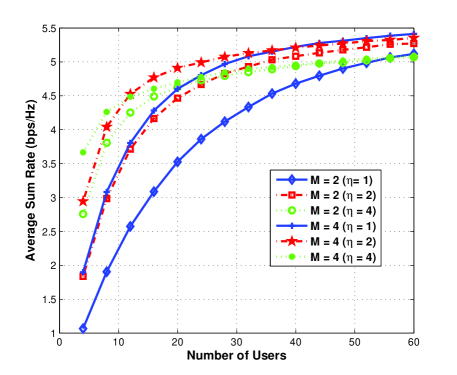
Figure 1: Comparison of average sum rate for different subband sizes ($\eta=1,2,4$) and partial feedback ($M=2,4$) with respect to the number of users. A general correlated channel model is assumed with an exponential power delay profile. ($N_{\mathsf{c}}=256$, $N=32$, $L=16$, $\delta=4$, $\frac{P_{\mathsf{c}}}{\sigma_{n_{\mathsf{c}}}^{2}}=10$ dB)

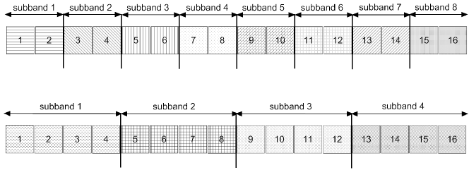
Figure 2: Illustration of the multi-cluster subband fading channel model for two different clusters with $16$ resource blocks. The subband sizes equal $2$ and $4$ for the two different clusters respectively. According to the subband fading model, the channel frequency selectivity is flat within each subband, and independent across subbands. The subband sizes can be heterogeneous across clusters, and this leads to heterogeneous channel frequency selectivity across clusters. The subband fading model approximates the general correlated channel model, and is useful for statistical analysis.

Now we demonstrate the need to adapt the subband size to achieve the potential “match” among coherence bandwidth, subband size and partial feedback through a simulation example. The channel is modeled according to the exponential power delay profile [36, 37, 38]: $\sigma_{l}^{2}=\frac{1-\exp(-1/\delta)}{1-\exp(-L/\delta)}\exp\left(-\frac{l}{\delta}\right)$ for $0\leq l<L$, where the parameter $\delta$ is related to the RMS delay spread. The simulation parameters are: $N_{\mathsf{c}}=256$, $N=32$, $L=16$, $\delta=4$, $\frac{P_{\mathsf{c}}}{\sigma_{n_{\mathsf{c}}}^{2}}=10$ dB. The subband size $\eta$ can be adjusted and ranges from $1$ to $4$ resource blocks. We consider partial feedback with $M=2$ and $M=4$. The average sum rate of the system for different subband sizes and partial feedback with respect to the number of users is shown in Fig. 1. Under the given coherence bandwidth, several observations can be made. Firstly, the curves with $\eta=4$ has the smallest increasing rate because a larger subband size gives a poor representation of the channel. Secondly, the curve with $\eta=1,M=2$ has the smallest average sum rate because a small amount of partial feedback is not enough to reflect the channel quality. Thirdly, the two curves $\eta=1,M=4$ and $\eta=2,M=2$ possess similar increasing rate. This is because the underlying channel is highly correlated within $2$ resource blocks and thus having $M$-best feedback with $\eta=2$ yields similar effect as having $2M$-best feedback with $\eta=1$. From the above observations, $\eta=2$ matches the frequency selectivity and there would be performance loss or waste of feedback resource when a subband size is blindly chosen. In a multi-cluster scenario where users in different clusters experience diverse coherence bandwidth, this advocates heterogeneous subband size and heterogeneous feedback.

The general correlated channel model as well as the non-linearity of the CQI, though useful to demonstrate the need for heterogeneous feedback, does not lend itself to tractable statistical analysis. To develop a tractable analytical framework, an approximated channel model is needed. A widely used model is the block fading model in the frequency domain [39, 40] due to its simplicity and capability to provide a good approximation to actual physical channels. According to the block fading model, the channel frequency selectivity is flat within each block, and independent across blocks [9, 17, 19]. Herein, we generalize the block fading model to the subband fading model for the multi-cluster scenario. We assume that users possessing similar frequency selectivity are grouped into a cluster and the subband size is perfectly matched to the coherence bandwidth for a given cluster. According to the subband fading model, for a given cluster with a perfectly matched subband size, the channel frequency selectivity is flat within each subband, and independent across subbands. Fig. 2 demonstrates the subband fading model for two different clusters with different subband sizes under a given number of resource blocks.

II-B Multi-Cluster Subband Fading Model

We now present the multi-cluster subband fading model. Consider a downlink multiuser OFDMA system with one base station and $G$ clusters of users. The system consists of $N$ resource blocks and the total number of users equals $K$. Users in cluster $\mathcal{K}_{g}$ are indexed by the set $\mathcal{K}_{g}=\{1,\ldots,k,\ldots,K_{g}\}$ for $1\leq g\leq G$, with $|\mathcal{K}_{g}|=K_{g}$ and $\sum_{g=1}^{G}K_{g}=K$. In our framework, users in the same cluster group their resource blocks into subbands in the same manner while each cluster can potentially employ a different grouping which enables the subband size to be heterogeneous between clusters. Denote $\eta_{g}$ as the subband size for cluster $\mathcal{K}_{g}$, and $\eta_{g}\in\{2^{0},2^{1},\ldots,N\}$. The $\eta_{g}$’s are ordered such that $\eta_{1}<\cdots<\eta_{G}$. Based on the assumption for $\eta_{g}$, the number of subbands in cluster $\mathcal{K}_{g}$ equals $\frac{N}{\eta_{g}}$.

Let $H_{k,r}^{(g)}$ be the frequency domain channel transfer function between transmitter and user $k$ in cluster $\mathcal{K}_{g}$ at subband $r$, where $1\leq k\leq K_{g},1\leq r\leq\frac{N}{\eta_{g}}$. $H_{k,r}^{(g)}$ is distributed as $\mathcal{CN}(0,1)$. According to the subband fading model, $H_{k,r}^{(g)}$ is assumed to be independent across users and subbands in cluster $\mathcal{K}_{g}$. The feedback for different clusters is at different granularity, and so to model the channel for the different clusters of users at the same basic resource block level, some additional notation is needed. Let $\tilde{H}_{k,n}^{(g)}=H_{k,\lceil\frac{n}{\eta_{g}}\rceil}^{(g)}$ with $1\leq n\leq N$ denote the resource block based channel transfer function. Then the received signals of user $k$ in cluster $\mathcal{K}_{g}$ at resource block $n$ can be represented by:

$$u_{k,n}^{(g)}=\sqrt{P}\tilde{H}_{k,n}^{(g)}s_{k,n}^{(g)}+v_{k,n}^{(g)},$$ (5)

where $P$ is the average received power per resource block, $s_{k,n}^{(g)}$ is the transmitted symbol and $v_{k,n}^{(g)}$ is additive white noise distributed with $\mathcal{CN}(0,\sigma_{n}^{2})$.

Let $Z_{k,r}^{(g)}\triangleq|H_{k,r}^{(g)}|^{2}$ denote the CQI for user $k$ in cluster $\mathcal{K}_{g}$ at subband $r$. In order to reduce the feedback load, users employ the best-M strategy to feed back their CQI. In the basic best-M feedback policy, users measure CQI for each resource block at their receiver and feed back the CQI values of the $M$ best resource blocks chosen from the total $N$ values. For each resource block, the scheduling policy selects the user with the largest CQI among the users who fed back CQI to the transmitter for that resource block. However, in our heterogeneous partial feedback framework, since the number of independent CQI for cluster $\mathcal{K}_{g}$ is $\frac{N}{\eta_{g}}$, a fair and reasonable way to allocate the feedback resource is to linearly scale the feedback amount for users in cluster $\mathcal{K}_{g}$. To be specific, user $k$ in $\mathcal{K}_{G}$ (i.e., the cluster with the largest subband size) is assumed to feed back the $M$ best CQI selected from $\{Z_{k,r}^{(G)}\},1\leq r\leq\frac{N}{\eta_{G}}$, whereas user $k$ in $\mathcal{K}_{g}$ conveys the $\frac{\eta_{G}}{\eta_{g}}M$ best CQI selected from $\{Z_{k,r}^{(g)}\},1\leq r\leq\frac{N}{\eta_{g}}$. After receiving feedback from all the clusters, for each resource block the system schedules the user for transmission with the largest CQI. It is useful to note that the user feedback is based on the subband level, while the base station schedules transmission at the resource block level.

III Perfect Feedback

In this section, the CQI are assumed to be fed back without any errors and the average sum rate is employed as the performance metric for system evaluation. We derive a closed form expression for the average sum rate in Section III-A for the multi-cluster heterogeneous feedback system. In Section III-B we analyze the relationship between the sum rate ratio and the choice of the best-M.

III-A Derivation of Average Sum Rate

According to the assumption, the CQI $Z_{k,r}^{(g)}$ is i.i.d. across subbands and users, and thus let $F_{Z}$ denote the CDF. Because only a subset of the ordered CQI are fed back, from the transmitter’s perspective, if it receives feedback on a certain resource block from a user, it is likely to be any one of the CQI from the ordered subset. We now aim to find the CDF of the CQI seen at the transmitter side as a consequence of partial feedback. Let $\tilde{Y}_{k,n}^{(g)}$ denote the reported CQI viewed at the transmitter for user $k$ in $\mathcal{K}_{g}$ at resource block $n$. Also, let $Y_{k,r}^{(g)}$ represent the subband-based CQI seen at the transmitter for user $k$ in $\mathcal{K}_{g}$ at subband $r$, then $\tilde{Y}_{k,n}^{(g)}=Y_{k,\lceil\frac{n}{\eta_{g}}\rceil}^{(g)}$. The following lemma describes the CDF of $\tilde{Y}_{k}^{(g)}$ (the index $n$ is dropped for notational simplicity), which is denoted by $F_{\tilde{Y}_{k}^{(g)}}$.

Lemma 1.

The CDF of $\tilde{Y}_{k}^{(g)}$ is given by:

$$F_{\tilde{Y}_{k}^{(g)}}(x)=\sum_{m=0}^{\frac{\eta_{G}}{\eta_{g}}M-1}\xi_{g}(N,M,\boldsymbol{\eta},m)(F_{Z}(x))^{\frac{N}{\eta_{g}}-m},$$ (6)

where the vector $\boldsymbol{\eta}\triangleq(\eta_{1},\cdots,\eta_{g},\cdots,\eta_{G})$ and

$$\xi_{g}(N,M,\boldsymbol{\eta},m)=\sum_{i=m}^{\frac{\eta_{G}}{\eta_{g}}M-1}\frac{\frac{\eta_{G}}{\eta_{g}}M-i}{\frac{\eta_{G}}{\eta_{g}}M}{\frac{N}{\eta_{g}}\choose i}{i\choose m}\left(-1\right)^{i-m}.$$ (7)

Proof.

The proof is provided in Appendix A. ∎

Let $k_{n}^{*}$ demote the selected user at resource block $n$, then according to the scheduling policy:

$$k_{n}^{*}=\arg\max_{k\in\mathcal{U}_{n}}\;\{\tilde{Y}_{k,n}^{(1)},\cdots,\tilde{Y}_{k,n}^{(g)},\cdots,\tilde{Y}_{k,n}^{(G)}\},$$ (8)

where $\mathcal{U}_{n}\triangleq\{\mathcal{U}_{n}^{(1)},\cdots,\mathcal{U}_{n}^{(g)},\cdots,\mathcal{U}_{n}^{(G)}\}$ is the set of users who convey feedback for resource block $n$, with $|\mathcal{U}_{n}^{(g)}|=\tau_{g}$ representing the number of users belonging to $\mathcal{U}_{n}$ in cluster $\mathcal{K}_{g}$. It can be easily seen that in the full feedback case, i.e., $M=M_{F}\triangleq\frac{N}{\eta_{G}}$, $|\mathcal{U}_{n}^{(g)}|=K_{g}$. For the general case when $1\leq M<M_{F}$, the probability mass function (PMF) of $\mathcal{U}_{n}$ is given by:

$$\mathbb{P}(\mathcal{U}_{n})=\left(\prod_{g=1}^{G}{K_{g}\choose\tau_{g}}\right)\left(\frac{\eta_{G}M}{N}\right)^{\sum_{g=1}^{G}\tau_{g}}\left(1-\frac{\eta_{G}M}{N}\right)^{K-\sum_{g=1}^{G}\tau_{g}},\quad 0\leq\tau_{g}\leq K_{g}.$$ (9)

Remark: Only the largest subband size $\eta_{G}$ appears in the expression of $\mathbb{P}(\mathcal{U}_{n})$ instead of the vector $\boldsymbol{\eta}$. This is due to our heterogeneous partial feedback design to let users in cluster $\mathcal{K}_{g}$ convey back the $\frac{\eta_{G}}{\eta_{g}}M$ best CQI out of $\frac{N}{\eta_{g}}$ values.

Now we turn to determine the conditional CDF of the CQI for the selected user at resource block $n$, conditioned on the set of users providing CQI for that resource block. Since users are equiprobable to be scheduled according to the fair scheduling policy, the condition on $k_{n}^{*}$ is not described explicitly, and so we denote the conditional CDF as $F_{X_{n}|\mathcal{U}_{n}}$, where $X_{n}|\mathcal{U}_{n}$ is the conditional CQI of the selected user at resource block $n$. Notice from Lemma 1 that $\tilde{Y}_{k}^{(g)}$ possess a different distribution for different $g$ due to the heterogeneous feedback from different clusters. Using order statistics [41] yields $F_{X_{n}|\mathcal{U}_{n}}$ as:

$$F_{X_{n}|\mathcal{U}_{n}}(x)=\prod_{g=1}^{G}(F_{\tilde{Y}_{k}^{(g)}}(x))^{\tau_{g}}.$$ (10)

Then the polynomial form of $F_{X_{n}|\mathcal{U}_{n}}$ can be obtained, which is stated in the following theorem.

Theorem 1.

The CDF of $F_{X_{n}|\mathcal{U}_{n}}$ is given by:

$$F_{X_{n}|\mathcal{U}_{n}}(x)=\sum_{m=0}^{\Phi(M,\boldsymbol{\eta},\boldsymbol{\tau})}\Theta_{G-1}(N,M,\boldsymbol{\eta},\boldsymbol{\tau},m)(F_{Z}(x))^{\sum_{g=1}^{G}\frac{N}{\eta_{g}}\tau_{g}-m},$$ (11)

where the vector $\boldsymbol{\tau}\triangleq(\tau_{1},\cdots,\tau_{g},\cdots,\tau_{G})$, $\Phi(M,\boldsymbol{\eta},\boldsymbol{\tau})\triangleq\sum_{g=1}^{G}\tau_{g}\left(\frac{\eta_{G}}{\eta_{g}}M-1\right)$,

$$\Theta_{g}(N,M,\boldsymbol{\eta},\boldsymbol{\tau},m)=\left\{\begin{array}[]{l}\mathop{\sum}\limits_{i=0}^{m}\Lambda_{1}(N,M,\boldsymbol{\eta},\boldsymbol{\tau},i)\Lambda_{2}(N,M,\boldsymbol{\eta},\boldsymbol{\tau},m-i),\quad g=1\\ \mathop{\sum}\limits_{i=0}^{m}\Theta_{g-1}(N,M,\boldsymbol{\eta},\boldsymbol{\tau},i)\Lambda_{g+1}(N,M,\boldsymbol{\eta},\boldsymbol{\tau},m-i),\quad 2\leq g<G\\ \end{array}\right.$$ (12)

$$\Lambda_{g}(N,M,\boldsymbol{\eta},\boldsymbol{\tau},m)=\left\{\begin{array}[]{l}(\xi_{g}(N,M,\boldsymbol{\eta},0))^{\tau_{g}},\quad m=0\\ \frac{1}{m\xi_{g}(N,M,\boldsymbol{\eta},0)}\sum_{\ell=1}^{\min\left(m,\frac{\eta_{G}}{\eta_{g}}M-1\right)}((\tau_{g}+1)\ell-m)\\ \times\xi_{g}(N,M,\boldsymbol{\eta},\ell)\Lambda_{g}(N,M,\boldsymbol{\eta},\boldsymbol{\tau},m-\ell),\quad 1\leq m<\tau_{g}(\frac{\eta_{G}}{\eta_{g}}M-1)\\ (\xi_{g}(N,M,\boldsymbol{\eta},\frac{\eta_{G}}{\eta_{g}}M-1))^{\tau_{g}},\quad m=\tau_{g}(\frac{\eta_{G}}{\eta_{g}}M-1).\\ \end{array}\right.$$ (13)

Proof.

The proof is provided in Appendix A. ∎

After obtaining the conditional CDF $F_{X_{n}|\mathcal{U}_{n}}$, let $C_{P}(M)$ denote the average sum rate and it can be computed using the following procedure.

$$C_{P}(M) =\frac{1}{N}\sum_{n=1}^{N}\mathbb{E}[\log_{2}(1+X_{n})]$$

$$\mathop{=}\limits^{(a)}\mathbb{E}_{\mathcal{U}}\left[\int_{0}^{\infty}\log_{2}(1+\rho x)d(F_{X|\mathcal{U}}(x))\right]$$

$$\mathop{=}\limits^{(b)}\mathbb{E}_{\mathcal{U}}\left[\sum_{m=0}^{\Phi(M,\boldsymbol{\eta},\boldsymbol{\tau})}\Theta_{G-1}(N,M,\boldsymbol{\eta},\boldsymbol{\tau},m)\int_{0}^{\infty}\log_{2}(1+\rho x)d(F_{Z}(x))^{\sum_{g=1}^{G}\frac{N}{\eta_{g}}\tau_{g}-m}\right]$$

$$\mathop{=}\limits^{(c)}\sum_{\boldsymbol{\tau}\neq\mathbf{0}}\mathbb{P}(\mathcal{U})\sum_{m=0}^{\Phi(M,\boldsymbol{\eta},\boldsymbol{\tau})}\Theta_{G-1}(N,M,\boldsymbol{\eta},\boldsymbol{\tau},m)\mathcal{I}_{1}\left(\rho,\sum_{g=1}^{G}\frac{N}{\eta_{g}}\tau_{g}-m\right),$$ (14)

where $\rho\triangleq\frac{P}{\sigma_{n}^{2}}$ and $\mathbb{P}(\mathcal{U})$ is given by (9). (a) follows from the conditional expectation of $X_{n}|\mathcal{U}_{n}$ and the identically distributed property (let $X$ and $\mathcal{U}$ represent $X_{n}$ and $\mathcal{U}_{n}$ respectively), (b) follows from (11) in Theorem 1, (c) follows from (9), and define $\mathcal{I}_{1}(a,b)\triangleq\int_{0}^{\infty}\log_{2}(1+ax)d(F_{Z}(x))^{b}$. $\mathcal{I}_{1}(a,b)$ is computed in Appendix A to be:

$$\mathcal{I}_{1}(a,b)=\frac{b}{\ln 2}\sum_{\ell=0}^{b-1}\binom{b-1}{\ell}\frac{(-1)^{\ell}}{\ell+1}\exp\left(\frac{\ell+1}{a}\right)E_{1}\left(\frac{\ell+1}{a}\right),$$ (15)

where $E_{1}(x)=\int_{x}^{\infty}\exp(-t)t^{-1}dt$ is the exponential integral function [42].

The average sum rate for the full feedback is a special case and is given by:

$$C_{P}(M_{F})=\int_{0}^{\infty}\log_{2}(1+\rho x)d(F_{Z}(x))^{K}=\mathcal{I}_{1}(\rho,K).$$ (16)

Remark: It is noteworthy to mention that the functional form of $C_{P}(M)$ in (14) consists of two main parts. The first part, which involves $\mathbb{P}(\mathcal{U})$ and $\Theta_{G-1}(\cdot,\cdot,\cdot,\cdot,\cdot)$, accounts for the randomness of the set of users who convey feedback as well as the scheduling policy. This part is inherent to the heterogeneous partial feedback strategy, and is independent of the system metric for evaluation, such as the average sum rate employed in this paper. The second part $\mathcal{I}_{1}(\cdot,\cdot)$ depends on statistical assumption of the underlying channel and the system metric, and it is impacted by partial feedback as well.

III-B Sum Rate Ratio and Best-M

We now examine how to determine the smallest $M$ that results in almost the same performance, in terms of average sum rate, as the full feedback case. Applying the same technique as in [15, 19], define $\gamma_{P}$ as the spectral efficiency ratio and the problem can be formulated as:

$$\mathrm{Find\;the\;minimum\;}M^{\ast},\quad s.t.\;\gamma_{P}=\frac{C_{P}(M^{\ast})}{C_{P}(M_{F})}\geq\gamma.$$ (17)

The above problem can be numerically solved by substituting the expressions for $C_{P}(M)$ and $C_{P}(M_{F})$. In order to obtain a simpler and tractable relationship between $M$ and $K$ given $\boldsymbol{\eta}$, i.e., the tradeoff between the amount of partial feedback and the number of users given existing heterogeneity of channel statistics in frequency domain, an approximation is utilized similar to that in [19], by observing that $\mathcal{I}_{1}(a,b)$ in (15) is slowly increasing in $b$ with fixed $a$ (This phenomenon is due to the saturation of multiuser diversity [43]). Observing $\sum_{m=0}^{\Phi(M,\boldsymbol{\eta},\boldsymbol{\tau})}\Theta_{G-1}(N,M,\boldsymbol{\eta},\boldsymbol{\tau},m)=1$ and employing the binomial theorem yields the approximation for the spectral efficiency ratio as:

$$\gamma_{P}\simeq 1-\left(1-\frac{\eta_{G}M^{\ast}}{N}\right)^{K}.$$ (18)

From (17) and (18), the minimum required $M^{\ast}$ can be obtained as follows:

$$M^{\ast}\geq\frac{N}{\eta_{G}}\left(1-\left(1-\gamma\right)^{\frac{1}{K}}\right).$$ (19)

Remark: It can be seen that $M^{*}$ depends on the system parameters ($N,K,\gamma$) as well on the largest subband size $\eta_{G}$. It is also a consequence of our heterogeneous partial feedback assumption to let users in cluster $\mathcal{K}_{g}$ convey back the $\frac{\eta_{G}}{\eta_{g}}M$ best CQI out of $\frac{N}{\eta_{g}}$ values. This results in the fact that obtaining feedback information from users belonging to different clusters have almost the same statistical influence on scheduling performance.

IV Imperfect Feedback

After analyzing the heterogeneous partial feedback design with perfect feedback, we turn to examine the impact of feedback imperfections in this section. We develop the imperfect feedback model due to channel estimation error and feedback delay in Section IV-A, and investigate the influence of imperfections on two different transmission strategies in Section IV-B and IV-C. Then we propose how to optimize the system performance to adapt to the imperfections in Section IV-D.

IV-A Imperfect Feedback Model

The imperfect feedback model is built upon the subband fading model for the perfect feedback case. To differentiate from the notation for the perfect feedback case and focus on the imperfect feedback model, the resource block index is dropped. Let $h_{k}$ denote the frequency domain channel transfer function of user $k$ (users in different clusters are not temporally distinguished to avoid notational overload). Due to channel estimation error, the user only has its estimated version $\hat{h}_{k}$, and the relationship between $h_{k}$ and $\hat{h}_{k}$ can be modeled as:

$$h_{k}=\hat{h}_{k}+w_{k},$$ (20)

where $w_{k}\sim\mathcal{CN}(0,\sigma_{w_{k}}^{2})$ is the channel estimation error. The channel of each resource block is assumed to be estimated independently, which yields the channel estimation errors $w_{k}$ i.i.d. across users and resource blocks, i.e., $w_{k}\sim\mathcal{CN}(0,\sigma_{w}^{2})$. It is clear that the base station makes decision on scheduling and adaptive transmission depending on CQI, a function of $\hat{h}_{k}$. Thus this information can be outdated due to delay between the instant CQI is measured and the actual instant of use for data transmission to the selected user. Let $\tilde{h}_{k}$ be the actual channel transfer function and we employ a first-order Gaussian-Markov model [27, 22, 25] to describe the time evolution and to capture the relationship with the delayed version as follows:

$$\tilde{h}_{k}=\alpha_{k}(\hat{h}_{k}+w_{k})+\sqrt{1-\alpha_{k}^{2}}\varepsilon_{k},$$ (21)

where $\varepsilon_{k}$ accounts for the innovation noise and is distributed as $\mathcal{CN}(0,1)$. The delay time between $\tilde{h}_{k}$ and $\hat{h}_{k}$ is not explicitly written for notational simplicity, and $\alpha_{k}\in[0,1]$ is used to model the correlation coefficient. Since the feedback delay is mainly caused by the periodic feedback interval and processing complexity [25], the innovation noise $\varepsilon_{k}$ are i.i.d. across users and a common $\alpha$ is assumed. Moreover, $w_{k}$ and $\varepsilon_{k}$ are assumed independent. Therefore, for notational simplicity, the user index $k$ in the aforementioned parameters is dropped and $\hat{Z}\triangleq|\hat{h}|^{2}$ is denoted as CQI.

Let $\tilde{\chi},\chi$ and $\hat{\chi}$ represent: the actual CQI of the selected user for transmission, its outdated version, and its outdated estimate respectively ($\hat{\chi}$ corresponds to $X$ for the perfect feedback case in Section III-A). Notice that the PDF of the outdated estimate $\hat{\chi}$ depends on the heterogeneous feedback design and the scheduling strategy, whereas the conditional PDF of $\tilde{\chi}|\hat{\chi}$ only depends on $\alpha$ and $\sigma_{w}^{2}$. Employing the same method in [26, 27], the conditional PDF is obtained as follows:

$$f_{\tilde{\chi}|\hat{\chi}}(x|\hat{\chi})=\frac{\alpha_{w}^{2}}{2}\exp\left(-\frac{\alpha_{w}^{2}x+\alpha_{w}^{2}\alpha^{2}\hat{\chi}}{2}\right)I_{0}(\alpha_{w}^{2}\alpha\sqrt{\hat{\chi}x}),$$ (22)

where $\alpha_{w}=\sqrt{\frac{2}{\alpha^{2}\sigma_{w}^{2}+1-\alpha^{2}}}$, and $I_{0}(\cdot)$ is the zeroth-order modified Bessel function of the first kind [42].

Since the feedback is imperfect, there are two types of issues that arise. The first is the choice of the incorrect user to serve. However, because of the i.i.d nature of the errors this does not compromise the fairness and also does not complicate the determination of the CDF. The second problem is that of outage because the rate adaptation is made by the base station based on the erroneous CQI. Because of the error in the CQI, the rate chosen may exceed the rate that the channel can support and so the base station has to take steps to mitigate this effect of outage. A conservative strategy will result in less outage but under utilization of the channel while an aggressive strategy will result in good utilization of the channel but only for a small fraction of the time. We now present two transmission strategies to address the outage issue.

IV-B Fix Rate Strategy

In the fix rate conservative scenario, a system parameter $\beta_{0}$ is chosen for rate adaptation, and outage results under the following condition:

$$\mathrm{Declare\;outage\;if:}\quad\{\tilde{\chi}\leq\beta_{0}|\hat{\chi}\}.$$ (23)

The system average goodput is defined as the total average bps/Hz successfully transmitted [23]. We derive the average goodput and average outage probability for a given choice of system parameter $\beta_{0}$ in the following procedure.

Firstly the conditional outage probability is expressed as:

$$\mathbb{P}(\tilde{\chi}\leq\beta_{0}|\hat{\chi})=1-\mathcal{Q}_{1}(\alpha_{w}\alpha\sqrt{\hat{\chi}},\alpha_{w}\sqrt{\beta_{0}}),$$ (24)

where $\mathcal{Q}_{1}(a,b)=\int_{b}^{\infty}t\exp(-\frac{t^{2}+a^{2}}{2})I_{0}(at)dt$ is the first-order Marcum-Q function [44]. Denote $R_{0}(\beta_{0},M)$ as the average goodput for the heterogeneous partial feedback system, which is written according to definition:

$$R_{0}(\beta_{0},M)=\mathbb{E}_{\mathcal{U}}\left[\mathbb{E}_{\hat{\chi}|\mathcal{U}}\left[\mathbb{P}(\tilde{\chi}\geq\beta_{0}|\hat{\chi})\log_{2}(1+\rho\beta_{0})\right]\right].$$ (25)

Then, from (9) and (14), $R_{0}(\beta_{0},M)$ can be computed as:

$$R_{0}(\beta_{0},M)$$

$$=\mathbb{E}_{\mathcal{U}}\left[\sum_{m=0}^{\Phi(M,\boldsymbol{\eta},\boldsymbol{\tau})}\Theta_{G-1}(N,M,\boldsymbol{\eta},\boldsymbol{\tau},m)\int_{0}^{\infty}\mathcal{Q}_{1}(\alpha_{w}\alpha\sqrt{x},\alpha_{w}\sqrt{\beta_{0}})\log_{2}(1+\rho\beta_{0})d(F_{\hat{Z}}(x))^{\sum_{g=1}^{G}\frac{N}{\eta_{g}}\tau_{g}-m}\right]$$

$$=\sum_{\boldsymbol{\tau}\neq\mathbf{0}}\mathbb{P}(\mathcal{U})\sum_{m=0}^{\Phi(M,\boldsymbol{\eta},\boldsymbol{\tau})}\Theta_{G-1}(N,M,\boldsymbol{\eta},\boldsymbol{\tau},m)\log_{2}(1+\rho\beta_{0})\mathcal{I}_{2}\left(\beta_{0},\sum_{g=1}^{G}\frac{N}{\eta_{g}}\tau_{g}-m\right),$$ (26)

where $\mathcal{I}_{2}(a,b)\triangleq\int_{0}^{\infty}\mathcal{Q}_{1}(\alpha_{w}\alpha\sqrt{x},\alpha_{w}\sqrt{a})d(F_{\hat{Z}}(x))^{b}$. $\mathcal{I}_{2}(a,b)$ is computed in Appendix B to be:

$$\mathcal{I}_{2}(a,b)=\frac{2b}{(1-\sigma_{w}^{2})\ln 2}\sum_{\ell=0}^{b-1}\binom{b-1}{\ell}(-1)^{\ell}\frac{1}{\zeta_{\ell}}\left(\exp(-\frac{\vartheta^{2}}{2})+\exp(-\frac{\zeta_{\ell}\vartheta^{2}}{2(\varpi^{2}+\zeta_{\ell})})(1-\exp(-\frac{\varpi^{2}\vartheta^{2}}{2(\varpi^{2}+\zeta_{\ell})}))\right),$$ (27)

where $\varpi=\alpha_{w}\alpha$, $\vartheta=\alpha_{w}\sqrt{a}$, $\zeta_{\ell}=\frac{2(\ell+1)}{1-\sigma_{w}^{2}}$.

The average outage probability $P_{0}(\beta_{0},M)$ for the heterogeneous partial feedback design can be directly calculated from definition and (26) as follows:

$$P_{0}(\beta_{0},M) =\mathbb{E}_{\mathcal{U}}\left[\mathbb{E}_{\hat{\chi}|\mathcal{U}}\left[\mathbb{P}(\tilde{\chi}\leq\beta_{0}|\hat{\chi})\right]\right]$$

$$=\sum_{\boldsymbol{\tau}\neq\mathbf{0}}\mathbb{P}(\mathcal{U})\sum_{m=0}^{\Phi(M,\boldsymbol{\eta},\boldsymbol{\tau})}\Theta_{G-1}(N,M,\boldsymbol{\eta},\boldsymbol{\tau},m)\left(1-\mathcal{I}_{2}\left(\beta_{0},\sum_{g=1}^{G}\frac{N}{\eta_{g}}\tau_{g}-m\right)\right).$$ (28)

The average goodput and average outage probability for the full feedback scenario is a special case and is given by:

$$R_{0}(\beta_{0},M_{F}) =\log_{2}(1+\rho\beta_{0})\mathcal{I}_{2}(\beta_{0},K),$$

$$P_{0}(\beta_{0},M_{F}) =1-\mathcal{I}_{2}(\beta_{0},K).$$ (29)

IV-C Variable Rate Strategy

Instead of choosing a conservative system parameter to account for the fix rate scenario as in the previous subsection, we consider an approach we refer to as the variable rate strategy. In the variable rate scenario, a system parameter $\beta_{1}$ is chosen and outage results under the following condition:

$$\mathrm{Declare\;outage\;if:}\quad\{\tilde{\chi}\leq\beta_{1}\hat{\chi}|\hat{\chi}\},$$ (30)

where $\beta_{1}$ can be regarded as the backoff factor. The system average goodput and average outage probability can be derived utilizing the following procedure.

Now under the variable rate scenario, the conditional outage probability is expressed as:

$$\mathbb{P}(\tilde{\chi}\leq\beta_{1}\hat{\chi}|\hat{\chi})=1-\mathcal{Q}_{1}(\alpha_{w}\alpha\sqrt{\hat{\chi}},\alpha_{w}\sqrt{\beta_{1}\hat{\chi}}).$$ (31)

Using the same method as (25) and (26), let $R_{1}(\beta_{1},M)$ denote the average goodput for the variable rate scenario whose expression can be written as follows:

$$R_{1}(\beta_{1},M) =\mathbb{E}_{\mathcal{U}}\left[\mathbb{E}_{\hat{\chi}|\mathcal{U}}\left[\mathbb{P}(\tilde{\chi}\geq\beta_{1}\hat{\chi}|\hat{\chi})\log_{2}(1+\rho\beta_{1}\hat{\chi})\right]\right]$$

$$=\sum_{\boldsymbol{\tau}\neq\mathbf{0}}\mathbb{P}(\mathcal{U})\sum_{m=0}^{\Phi(M,\boldsymbol{\eta},\boldsymbol{\tau})}\Theta_{G-1}(N,M,\boldsymbol{\eta},\boldsymbol{\tau},m)\mathcal{I}_{3}\left(\beta_{1},\sum_{g=1}^{G}\frac{N}{\eta_{g}}\tau_{g}-m\right),$$ (32)

where $\mathcal{I}_{3}(a,b)\triangleq\int_{0}^{\infty}\mathcal{Q}_{1}(\alpha_{w}\alpha\sqrt{x},\alpha_{w}\sqrt{ax})\log_{2}(1+\rho ax)d(F_{\hat{Z}}(x))^{b}$.

For the full feedback case, the average goodput is given by:

$$R_{1}(\beta_{1},M_{F})=\mathcal{I}_{3}(\beta_{1},K).$$ (33)

Note that unlike $\mathcal{I}_{2}(a,b)$, $\mathcal{I}_{3}(a,b)$ can not be written in closed form. Therefore, bounding technique and suitable approximation are attractive to find closed form alternatives for $\mathcal{I}_{3}(a,b)$. The following proposition presents a valid closed form upper bound for $\mathcal{I}_{3}(a,b)$ in the low $\mathsf{SNR}$ regime.

Proposition 1.

In the low $\mathsf{SNR}$ regime, $\mathcal{I}_{3}(a,b)$ can be efficiently upper bounded by:

$$\mathcal{I}_{3}^{\mathrm{UB}}(a,b)= \frac{4\rho ab}{(1-\sigma_{w}^{2})\ln 2}\sum_{\ell=0}^{b-1}(-1)^{\ell}\frac{1}{\zeta_{\ell}^{2}}\Bigg{(}1+\frac{\vartheta^{2}}{\varphi_{\ell}}\Bigg{(}\frac{\varpi^{2}}{\varphi_{\ell}}{}_{2}F_{1}\left(1,\frac{3}{2};2;\frac{4\varpi^{2}\vartheta^{2}}{\varphi_{\ell}^{2}}\right)-{}_{2}F_{1}\left(\frac{1}{2},1;1;\frac{4\varpi^{2}\vartheta^{2}}{\varphi_{\ell}^{2}}\right)$$

$$+\frac{2\zeta_{\ell}}{\varphi_{\ell}}\Bigg{(}\frac{\varpi^{2}}{\varphi_{\ell}}{}_{2}F_{1}\left(\frac{3}{2},2;2;\frac{4\varpi^{2}\vartheta^{2}}{\varphi_{\ell}^{2}}\right)-\frac{1}{2}{}_{2}F_{1}\left(1,\frac{3}{2};1;\frac{4\varpi^{2}\vartheta^{2}}{\varphi_{\ell}^{2}}\right)\Bigg{)}\Bigg{)}\Bigg{)},$$ (34)

where $\varpi=\alpha_{w}\alpha$, $\vartheta=\alpha_{w}\sqrt{a}$, $\zeta_{\ell}=\frac{2(\ell+1)}{1-\sigma_{w}^{2}}$, $\varphi_{\ell}=\varpi^{2}+\vartheta^{2}+\zeta_{\ell}$, and ${}_{2}F_{1}(\cdot,\cdot;\cdot;\cdot)$ is the Gaussian hypergeometric function [42].

Proof.

The proof is provided in Appendix B. ∎

$\mathcal{I}_{3}^{\mathrm{UB}}(a,b)$ is valid and tight especially for the low $\mathsf{SNR}$ regime. In order to track $\mathcal{I}_{3}(a,b)$ over the whole $\mathsf{SNR}$ regimes, we propose the following approximation method by leveraging Jensen’s inequality [45]. Recall the definition of $\mathcal{I}_{3}(a,b)=\mathbb{E}[\mathcal{Q}_{1}(\alpha_{w}\alpha\sqrt{\check{\chi}},\alpha_{w}\sqrt{a\check{\chi}})\log_{2}(1+\rho a\check{\chi})]$, where the random variable $\check{\chi}$ is defined to have CDF $(F_{\hat{Z}}(x))^{b}$. Firstly, $\mathbb{E}[\check{\chi}]$ can be computed and is given by:

$$\mathbb{E}[\check{\chi}] =\int_{0}^{\infty}x\frac{b}{1-\sigma_{w}^{2}}\sum_{\ell=0}^{b-1}\binom{b-1}{\ell}(-1)^{\ell}\exp\left({-\frac{(\ell+1)x}{1-\sigma_{w}^{2}}}\right)dx$$

$$=\frac{b}{1-\sigma_{w}^{2}}\sum_{\ell=0}^{b-1}\binom{b-1}{\ell}(-1)^{\ell}\left(\frac{1-\sigma_{w}^{2}}{\ell+1}\right)^{2}.$$ (35)

Then plugging (35) into $\mathcal{Q}_{1}(\alpha_{w}\alpha\sqrt{x},\alpha_{w}\sqrt{ax})\log_{2}(1+\rho ax)$ yields:

$$\mathcal{I}_{3}^{A}(a,b)=\mathcal{Q}_{1}\left(\alpha_{w}\alpha\sqrt{\mathbb{E}[\check{\chi}]},\alpha_{w}\sqrt{a\mathbb{E}[\check{\chi}]}\right)\log_{2}(1+\rho a\mathbb{E}[\check{\chi}]).$$ (36)

Note that $\mathcal{I}_{3}^{A}(a,b)$ would serve as an upper bound from Jensen’s inequality if the function of interest $\mathcal{Q}_{1}(\alpha_{w}\alpha\sqrt{x},\alpha_{w}\sqrt{ax})\log_{2}(1+\rho ax)$ was concave in $x$. Properties of this function such as monotonicity and concavity are of interest and lead to rigorous arguments in support of this bound. If outage does not occur, extensive analysis can be carried out due to the well known properties of the $\log(\cdot)$ function. However, the concavity (or log-concavity) of $\mathcal{Q}_{1}(\alpha_{w}\alpha\sqrt{x},\alpha_{w}\sqrt{\beta_{1}x})$ in $x$ (notice that $x$ appears in both entries of $\mathcal{Q}_{1}(\cdot,\cdot)$) still remains an important open problem [46]. Our numerical evidence suggests that $\mathcal{Q}_{1}(\alpha_{w}\alpha\sqrt{x},\alpha_{w}\sqrt{\beta_{1}x})\log_{2}(1+\rho\beta_{1}x)$ is concave and monotonically increasing in $x$ for practical choices of $\beta_{1}$. For any given $\beta_{1}$ preserving the aforementioned property, Jensen’s inequality yields an upper bound, whose tightness is of interest and discussed in the following proposition. The word practical is used to exclude the situation when $\beta_{1}$ approaches its maximum $1$ which in turn enables $\mathcal{Q}_{1}(\cdot,\cdot)$ to dominate the goodput to incur extreme outage. This makes intuitive sense according to the definition of average goodput.

Proposition 2.

Let $\{\check{\chi}_{b}\}$ be the family of positive i.i.d. random variables. If $\mathcal{Q}_{1}(\alpha_{w}\alpha\sqrt{x},\alpha_{w}\sqrt{\beta_{1}x})\log_{2}(1+\rho\beta_{1}x)$ is concave and monotonically increasing in $x$ for any given $\beta_{1}$, then the Jensen bound is asymptotically tight, i.e., as $b\rightarrow\infty$,

$$\frac{\mathbb{E}[\mathcal{Q}_{1}(\alpha_{w}\alpha\sqrt{\check{\chi}_{b}},\alpha_{w}\sqrt{\beta_{1}\check{\chi}_{b}})\log_{2}(1+\rho\beta_{1}\check{\chi}_{b})]}{\mathcal{Q}_{1}(\alpha_{w}\alpha\sqrt{\mathbb{E}[\check{\chi}_{b}]},\alpha_{w}\sqrt{\beta_{1}\mathbb{E}[\check{\chi}_{b}]})\log_{2}(1+\rho\beta_{1}\mathbb{E}[\check{\chi}_{b}])}\rightarrow 1.$$ (37)

Proof.

The proof is provided in Appendix B. ∎

Nonetheless, when the aforementioned property is not preserved (e.g., $\beta_{1}$ approaches $1$), Jensen’s inequality does not hold but the expression has been experimentally found to be a good approximation and so can still be used. Therefore, (36) is denoted as Jensen approximation. We conduct a numerical study and demonstrate the tightness of Jensen approximation in Fig. 3. It is observed that the approximation method is very tight for moderate (even small) number of users and for all values of $\beta_{1}\in[0,1]$, which shows its potential in accurately tracking the performance of average goodput.

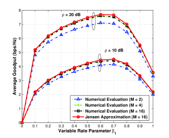
Figure 3: Calculating the average goodput from numerical evaluation ($M=2,4,16$) and Jensen approximation ($M=16$) for the variable rate scenario under different $\rho$. ($N=64$, $\boldsymbol{\eta}=(1,4)$, $K_{1}=K_{2}=K/2=10$, $\alpha=0.98$, $\sigma_{w}^{2}=0.01$, $\rho=10$ dB, and $20$ dB)

Now we calculate the average outage probability. Since it does not involve the $\log(\cdot)$ function, it can be computed into closed form as follows:

$$P_{1}(\beta_{1},M) =\mathbb{E}_{\mathcal{U}}\left[\mathbb{E}_{\hat{\chi}|\mathcal{U}}\left[\mathbb{P}(\tilde{\chi}\leq\beta_{1}\hat{\chi}|\hat{\chi})\right]\right]$$

$$=\sum_{\boldsymbol{\tau}\neq\mathbf{0}}\mathbb{P}(\mathcal{U})\sum_{m=0}^{\Phi(M,\boldsymbol{\eta},\boldsymbol{\tau})}\Theta_{G-1}(N,M,\boldsymbol{\eta},\boldsymbol{\tau},m)\left(1-\mathcal{I}_{4}\left(\beta_{1},\sum_{g=1}^{G}\frac{N}{\eta_{g}}\tau_{g}-m\right)\right),$$ (38)

where

$$\mathcal{I}_{4}(a,b) \triangleq\int_{0}^{\infty}\mathcal{Q}_{1}(\alpha_{w}\alpha\sqrt{x},\alpha_{w}\sqrt{ax})d(F_{\hat{Z}}(x))^{b}$$

$$\mathop{=}\limits^{(a)}\frac{2b}{(1-\sigma_{w}^{2})}\sum_{\ell=0}^{b-1}\binom{b-1}{\ell}(-1)^{\ell}\int_{0}^{\infty}\mathcal{Q}_{1}(\alpha_{w}\alpha x,\alpha_{w}\sqrt{a}x)\exp\left(-\frac{(\ell+1)x^{2}}{1-\sigma_{w}^{2}}\right)xdx$$

$$\mathop{=}\limits^{(b)}\frac{b}{(1-\sigma_{w}^{2})}\sum_{\ell=0}^{b-1}\binom{b-1}{\ell}(-1)^{\ell}\frac{1}{\zeta_{\ell}}\left(1+\frac{\psi_{\ell}}{\varsigma_{\ell}}\right),$$ (39)

$\varpi=\alpha_{w}\alpha$, $\vartheta=\alpha_{w}\sqrt{a}$, $\zeta_{\ell}=\frac{2(\ell+1)}{1-\sigma_{w}^{2}}$, $\varphi_{\ell}=\varpi^{2}+\vartheta^{2}+\zeta_{\ell}$, $\psi_{\ell}=\varpi^{2}-\vartheta^{2}+\zeta_{\ell}$, $\varsigma_{\ell}=\sqrt{\varphi_{\ell}^{2}-4\varpi^{2}\vartheta^{2}}$. (a) follows from change of variables; (b) follows from applying [47, B.48].

In the case of full feedback, the average outage probability $P_{1}(\beta_{1},M_{F})$ becomes:

$$P_{1}(\beta_{1},M_{F})=1-\mathcal{I}_{4}(\beta_{1},K).$$ (40)

IV-D Optimization and Adaptation to Imperfections

We have obtained the relationship between the system parameter ($\beta_{0}$ or $\beta_{1}$) and the system average goodput, and we now aim to maximize the average goodput by adapting the system parameters.

Consider the optimization of $R_{1}(\beta_{1},M)$ to obtain the optimal backoff factor $\beta_{1}^{\ast}$. It is observed from (IV-C) that directly optimizing $R_{1}(\beta_{1},M)$ is tedious, and a near-optimal method is now proposed to obtain $\beta_{1}^{\ast}$. This method is inspired by the results in Section III-B, which show that the minimum required $M^{\ast}$ can be chosen to achieve almost the same performance as a system with full feedback. Thus an optimal $\beta_{1}^{\ast}$ for the full feedback scenario can be optimized first, and then $M^{\ast}$ is obtained to “match” the system performance. Looking again at Fig. 3 with emphasis on different number $M$ of partial feedback, as $M$ gets larger, the optimal $\beta_{1}$ converges to the full feedback case. In this example, $M^{\ast}=4$ is adequate to match the system performance. It is noteworthy to mention that this adaptation philosophy can be applied to partial feedback systems wherein system parameters are optimized according to full feedback assumption first and minimum required partial feedback is chosen subsequently.

Note that a closed form approximation has been obtained to track $R_{1}(\beta_{1},M_{F})$ in Section IV-C, which is denoted as $R_{1}^{A}(\beta_{1},M_{F})\triangleq\mathcal{I}_{3}^{\mathrm{A}}(\beta_{1},K)$. The following proposition demonstrates the optimal property of $\beta_{1}$ when optimizing $R_{1}^{A}(\beta_{1},M_{F})$.

Proposition 3.

There exists a unique global optimal $\beta_{1}$ that maximizes $R_{1}^{A}(\beta_{1},M_{F})$.

Proof.

The proof is provided in Appendix B. ∎

From the above analysis, the optimization strategy can be described as:

$$\beta_{1}^{\ast}=\arg\mathop{\max}\limits_{0\leq\beta_{1}\leq 1}R_{1}^{A}(\beta_{1},M_{F})\simeq\arg\mathop{\max}\limits_{0\leq\beta_{1}\leq 1}R_{1}(\beta_{1},M_{F}).$$ (41)

Since it is proved in Proposition 3 that $R_{1}^{A}(\beta_{1},M_{F})$ is quasiconcave [45] in $\beta_{1}$, numerical approach such as Newton-Raphson method can be applied to obtain $\beta_{1}^{\ast}$. As discussed before, once $\beta_{1}^{*}$ is found, the minimum required $M^{*}$ can be obtained by solving (17) or relying on (19).

The same strategy can be carried over to the optimization of $\beta_{0}$, which is presented as follows:

$$\beta_{0}^{\ast}=\arg\mathop{\max}\limits_{\beta_{0}}R_{0}(\beta_{0},M_{F}).$$ (42)

The impact of imperfections on system parameter adaptation, and the comparison between the fixed rate and variable rate strategies will be examined through simulations in Section V-B.

V Numerical Results

In this section, we conduct a numerical study to verify the results developed and to draw some insight.

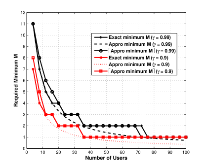
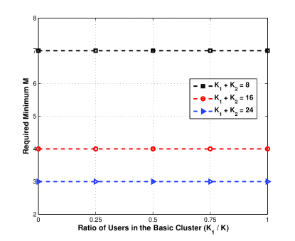
(a)	(b)

Figure 4: The required minimum $M$ for heterogeneous perfect feedback design: (a) Comparison of the required minimum $M$ between numerically solving (17) and using approximation (19) under different $\gamma$ with respect to the number of users; ($N=64$, $\boldsymbol{\eta}=(1,4)$, $K_{1}=K_{2}=K/2$, $\rho=10$ dB) (b) Computing the required minimum $M$ with respect to different number of users when varying the ratio of the number of users in cluster $\mathcal{K}_{1}$. ($N=64$, $\boldsymbol{\eta}=(1,4)$, $\rho=10$ dB, $\gamma=0.99$)

V-A Perfect Feedback Scenario

The number of resource blocks $N$ is assumed to be $64$ for simulations throughout this section. We first consider a $2$-cluster system. Fig. 4 (a) plots the minimum required $M$ obtained by directly solving (17) and alternatively by the approximation (19) for two thresholds: $\gamma=0.99$ and $0.9$. Note that the result from (19) is rounded with the ceiling function since the required $M$ is an integer. The other simulation parameters are $\boldsymbol{\eta}=(1,4)$ (i.e., $M_{F}=16$), and $\rho=10$ dB. It is observed that the results from the approximate expression matches quite well with the exact computation. The question of whether the required $M$ is sensitive to the partition of users in the system is examined in Fig. 4 (b) wherein the ratio of the number of users in cluster $\mathcal{K}_{1}$ is changed and the minimum required $M$ is depicted for different total number of users with threshold $\gamma=0.99$. Interestingly, the result turns out to be “uniform”. As discussed in Section III, it is due to the heterogenous feedback design assumption to let users in cluster $\mathcal{K}_{1}$ consume $\frac{\eta_{G}}{\eta_{1}}M$ ($4M$ in this simulation) feedback which results in the fact that obtaining feedback information from users belonging to different clusters have almost the same influence on scheduling performance. Therefore, the representative simulation setup $K_{g}=K/G$ can be employed when the system performance metric is investigated with respect to the total number of users.

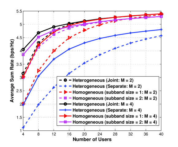
Figure 5: Comparison of the average sum rate for a $4$-cluster system under different feedback strategies with respect to the number of users ($N=64$, $\boldsymbol{\eta}=(1,2,4,8)$, $K_{1}=K_{2}=K_{3}=K_{4}=K/4$, $M=2,4$, $\rho=10$ dB)

We now consider a $4$-cluster system with subband size vector $\boldsymbol{\eta}=(1,2,4,8)$ (i.e., $M_{F}=8$). Fig. 5 demonstrates the benefit of using heterogeneous feedback design. One of the competing strategies is also heterogeneous, but treats users from each cluster separately. In particular, the system firstly clusters the users based on their channel statistics, and then serves the clusters one by one requiring feedback only from the served cluster of users. In this way, the feedback amount is varying over time depending on the partition of users. This strategy is denoted as separate heterogeneous feedback compared to our joint heterogeneous feedback design. The other competing strategies are homogeneous without taking advantage of the channel statistics of different users. To maintain at least the same feedback amount for fair comparison, each user in the homogeneous case is assumed to feed back $\lceil\sum_{g=1}^{G}\frac{\eta_{G}}{\eta_{g}}\frac{M}{G}\rceil$ CQI values. Two subband sizes are assumed for the homogeneous feedback. It is clear that for the homogeneous case, users in cluster $\mathcal{K}_{1}$ have more independent feedback while users in cluster $\mathcal{K}_{4}$ suffer from redundant feedback. The average sum rate for two different values of $M$ are shown in Fig. 5. The separate heterogenous feedback is observed to have the worst performance from a sum rate perspective because it does not fully exploit multiuser diversity, but it consumes the least feedback. Our joint heterogenous feedback design is shown to perform much better than the two homogeneous strategies for the $4$-cluster system. It is due to the fact that by considering the existing heterogeneity among users, the proposed heterogeneous design can make the best use of the degrees of freedom in the frequency domain in order to enhance the system performance as well as reduce feedback needs.

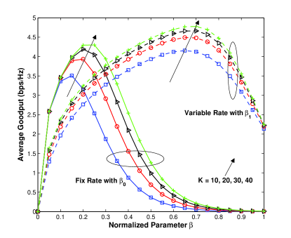
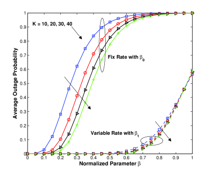
(a)	(b)

Figure 6: Comparison of fixed rate and variable rate strategies under normalized parameter $\beta$ ($\beta=\beta_{1}=\beta_{0}/10$) for different number of users $K$ ($N=64$, $\alpha=0.98$, $\sigma_{w}^{2}=0.01$, $\rho=10$ dB): (a) Comparison of average goodput; (b) Comparison of average outage probability.

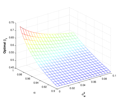
(a)	(b)

Figure 7: The effect of channel estimation error ($\sigma_{w}^{2}$) and feedback delay ($\alpha$) on the optimal value of $\beta_{0}$ and $\beta_{1}$ ($\rho=10$ dB, $K=10$, $\sigma_{w}^{2}=0:0.005:0.1$, $\alpha=0.9:0.005:0.99$): (a) The optimal fix rate parameter $\beta_{0}$ with respect to $\sigma_{w}^{2}$ and $\alpha$; (b) The optimal variable rate parameter $\beta_{1}$ with respect to $\sigma_{w}^{2}$ and $\alpha$.

V-B Imperfect Feedback Scenario

Fig. 6 exhibits the comparison between the fix rate and variable rate outage scenarios as well as the effect of the number of users on the optimization of $\beta_{0}$ and $\beta_{1}$. In order to show the system performance of the two scenarios in one figure, a normalized parameter $\beta$ is defined. While examining the variable rate plots $\beta=\beta_{1},$ and when considering the fixed rate plots $\beta=\beta_{0}/10$. The system parameters are: $\alpha=0.98$, $\sigma_{w}^{2}=0.01$, and $\rho=10$ dB. It can be seen that for both scenarios, larger number of users $K$ yields better system performance, i.e., higher average goodput and lower average outage probability. This is a consequence of increased multiuser diversity gain to combat the imperfections in the feedback system.

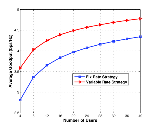
Figure 8: Comparison of the average goodput for a $4$-cluster system with fix rate and variable rate strategies using optimized $\beta_{0}^{*}$ and $\beta_{1}^{*}$. The average goodput is calculated using the best-M partial feedback scheme when the minimum required $M^{*}$ is computed after obtaining $\beta_{0}^{*}$ or $\beta_{1}^{*}$. ($N=64$, $\boldsymbol{\eta}=(1,2,4,8)$, $K_{1}=K_{2}=K_{3}=K_{4}=K/4$, $\alpha=0.98$, $\sigma_{w}^{2}=0.01$, $\rho=10$ dB)

Fig. 7 illustrates the effect of channel estimation error $\sigma_{w}^{2}$ and feedback delay $\alpha$ on the optimal value of $\beta_{0}$ and $\beta_{1}$. Here $\sigma_{w}^{2}$ is varied from $0$ to $0.1$, and $\alpha$ is varied from $0.9$ to $0.99$ in steps of $0.005$. It can be observed from the changing profiles that both the optimal values of $\beta_{0}$ and $\beta_{1}$ get smaller as the imperfections become worse. Therefore, the system should adjust the system parameters to adapt to the encountered imperfections.

Now we consider the adaptation of system parameters ($\beta_{0}$ or $\beta_{1}$) and partial feedback in a $4$-cluster heterogeneous feedback system. The system parameters are: $\boldsymbol{\eta}=(1,2,4,8)$, $\alpha=0.98$, $\sigma_{w}^{2}=0.01$, and $\rho=10$ dB. For both transmission strategies and for a given number of users $K$, the optimal value of $\beta_{0}^{*}$ or $\beta_{1}^{*}$ is first optimized according to the full feedback case discussed in Section IV-D. Then, a minimum required $M^{*}$ is obtained by matching the system performance to that in the full feedback case. Fig. 8 demonstrates the average goodput for both transmission strategies with $M^{*}$ and $\beta_{0}^{*}$ (or $\beta_{1}^{*}$). We observe that there is almost a constant performance gain for the variable rate strategy compared with the fix rate one. This is due to the fact that for the variable rate scenario, the system is adapting the transmission parameters conditioned on the past memory even if it is the outdated one. If the channel estimation error and feedback delay are not severe, the imperfections can be compensated by multiplying with the backoff factor and relying on the past feedback.

VI Conclusion

In this paper, we propose and analyze a heterogeneous feedback design adapting the feedback resource according to users’ frequency domain channel statistics. Under the general correlated channel model, we demonstrate the gain by achieving the potential match among coherence bandwidth, subband size and partial feedback. To facilitate statistical analysis, we employ the subband fading model for the multi-cluster heterogeneous feedback system. We derive a closed form expression of the average sum rate under perfect partial feedback assumption, and provide a method to obtain the minimum heterogeneous partial feedback required to obtain performance comparable to a scheme using full feedback. We also analyze the effect of imperfections on the heterogeneous partial feedback system. We obtain a closed form expression for the average goodput of the fix rate scenario, and utilize a bounding technique and tight approximation to track the performance of the variable rate scenario. Methods adapting the system parameters to maximize the average system goodput are proposed. The heterogeneous feedback design is shown to outperform the homogeneous one with the same feedback resource. With imperfections, the system adjusting the transmission strategy and the amount of partial feedback is shown to yield better performance. The developed analysis provides a theoretical reference to understand the approximate behavior of the proposed heterogeneous feedback system and its interplay with practical imperfections. Dealing with the general channel correlation and the corresponding nonlinear nature of the CQI are interesting directions for the heterogeneous feedback system.

Appendix A

Proof (sketch) of Lemma 1: The methodology is an extension of the work in [19] which deals with the homogeneous feedback case with one cluster of users and one specific subband size.

Let $F_{Y_{k}^{(g)}}$ denote the CDF of $Y_{k}^{(g)}\triangleq Y_{k,r}^{(g)}$. Substituting the subband size $\frac{N}{\eta_{g}}$ and the number of reported CQI $\frac{\eta_{G}}{\eta_{g}}M$ for user $k$ in cluster $\mathcal{K}_{g}$ makes $F_{Y_{k}^{(g)}}$ satisfy (6). It can be shown that $F_{\tilde{Y}_{k}^{(g)}}(x)=\mathbb{P}(\tilde{Y}_{k,n}^{(g)}\leq x)=\mathbb{P}(Y_{k,\lceil\frac{n}{\eta_{g}}\rceil}^{(g)}\leq x)=F_{Y_{k}^{(g)}}(x)$, which concludes the proof.

Proof of Theorem 1: Substituting the expressions of $F_{\tilde{Y}_{k}^{(g)}}$ from Lemma 1 and combining (10) yield:

$$F_{X_{n}|\mathcal{U}_{n}}(x)=(F_{Z}(x))^{\sum_{g=1}^{G}\frac{N}{\eta_{g}}\tau_{g}}\prod_{g=1}^{G}\left(\sum_{m=0}^{\frac{\eta_{G}}{\eta_{g}}M-1}\frac{\xi_{g}(N,M,\boldsymbol{\eta},0)}{(F_{Z}(x))^{m}}\right)^{\tau_{g}}.$$ (43)

Applying [48, 0.314] to a finite-order power series in (43), $\left(\sum_{m=0}^{\frac{\eta_{G}}{\eta_{g}}M-1}\frac{\xi_{g}(N,M,\boldsymbol{\eta},0)}{(F_{Z}(x))^{m}}\right)^{\tau_{g}}$ can be expressed as $\sum_{m=0}^{\tau_{g}(\frac{\eta_{G}}{\eta_{g}}M-1)}\frac{\Lambda_{g}(N,M,\boldsymbol{\eta},\boldsymbol{\tau},m)}{(F_{Z}(x))^{m}}$, where the expression for $\Lambda_{g}(N,M,\boldsymbol{\eta},\boldsymbol{\tau},m)$ is described in Theorem 1. Note that the coefficients of $\frac{1}{(F_{Z}(x))^{m}}$ can be computed in a recursive manner.

Then we employ [48, 0.316] for the multiplication of power series. For $g=1$, $\Theta_{1}(N,M,\boldsymbol{\eta},\boldsymbol{\tau},m)$ can be calculated from $\Lambda_{1}(N,M,\boldsymbol{\eta},\boldsymbol{\tau},m)$ and $\Lambda_{2}(N,M,\boldsymbol{\eta},\boldsymbol{\tau},m)$ as:

$$\Theta_{1}(N,M,\boldsymbol{\eta},\boldsymbol{\tau},m)=\mathop{\sum}\limits_{i=0}^{m}\Lambda_{1}(N,M,\boldsymbol{\eta},\boldsymbol{\tau},i)\Lambda_{2}(N,M,\boldsymbol{\eta},\boldsymbol{\tau},m-i).$$

For $2\leq g<G$, $\Theta_{g}(N,M,\boldsymbol{\eta},\boldsymbol{\tau},m)$ can be computed from $\Theta_{g-1}(N,M,\boldsymbol{\eta},\boldsymbol{\tau},m)$ and $\Lambda_{g+1}(N,M,\boldsymbol{\eta},\boldsymbol{\tau},m)$ in the following manner:

$$\Theta_{g}(N,M,\boldsymbol{\eta},\boldsymbol{\tau},m)=\mathop{\sum}\limits_{i=0}^{m}\Theta_{g-1}(N,M,\boldsymbol{\eta},\boldsymbol{\tau},i)\Lambda_{g+1}(N,M,\boldsymbol{\eta},\boldsymbol{\tau},m-i).$$

This concludes the proof.

Derivation of $\mathcal{I}_{1}(a,b)$: From the definition of $Z$, $F_{Z}(x)=1-\exp(-x)$ and $f_{Z}(x)=\exp(-x)$. Thus $d(F_{Z}(x))^{b}=b(F_{Z}(x))^{b-1}f_{Z}(x)dx=b\sum_{\ell=0}^{b-1}\binom{b-1}{\ell}(-1)^{\ell}\exp(-(\ell+1)x)dx$, where the last equality follows from the binomial theorem.

Therefore, $\int_{0}^{\infty}\log_{2}(1+ax)d(F_{Z}(x))^{b}=\frac{b}{\ln 2}\sum_{\ell=0}^{b-1}\binom{b-1}{\ell}(-1)^{\ell}\int_{0}^{\infty}\ln(1+ax)\exp(-(\ell+1)x)dx$. Applying [48, 4.337.2] yields (15).

Appendix B

Derivation of $\mathcal{I}_{2}(a,b)$: From the definition of $\hat{Z}$, it can be shown that $F_{\hat{Z}}(x)=1-\exp(-\frac{1}{1-\sigma_{w}^{2}}x)$ and $f_{\hat{Z}}(x)=\frac{1}{1-\sigma_{w}^{2}}\exp(-\frac{1}{1-\sigma_{w}^{2}}x)$. Then $\mathcal{I}_{2}(a,b)$ can be calculated as:

$$\mathcal{I}_{2}(a,b) \mathop{=}\limits^{(a)}\frac{2b}{(1-\sigma_{w}^{2})\ln 2}\sum_{\ell=0}^{b-1}\binom{b-1}{\ell}(-1)^{\ell}\int_{0}^{\infty}\mathcal{Q}_{1}(\alpha_{w}\alpha x,\alpha_{w}\sqrt{a})\exp\left(-\frac{(\ell+1)x^{2}}{1-\sigma_{w}^{2}}\right)xdx$$

$$\mathop{=}\limits^{(b)}\frac{2b}{(1-\sigma_{w}^{2})\ln 2}\sum_{\ell=0}^{b-1}\binom{b-1}{\ell}(-1)^{\ell}\frac{1}{\zeta_{\ell}}\left(\mathcal{Q}_{1}(0,\vartheta)+\exp(-\frac{\zeta_{\ell}\vartheta^{2}}{2(\varpi^{2}+\zeta_{\ell})})(1-\mathcal{Q}_{1}(0,\frac{\varpi\vartheta}{\sqrt{\varpi^{2}+\zeta_{\ell}}}))\right)$$

$$\mathop{=}\limits^{(c)}\frac{2b}{(1-\sigma_{w}^{2})\ln 2}\sum_{\ell=0}^{b-1}\binom{b-1}{\ell}(-1)^{\ell}\frac{1}{\zeta_{\ell}}\left(\exp(-\frac{\vartheta^{2}}{2})+\exp(-\frac{\zeta_{\ell}\vartheta^{2}}{2(\varpi^{2}+\zeta_{\ell})})(1-\exp(-\frac{\varpi^{2}\vartheta^{2}}{2(\varpi^{2}+\zeta_{\ell})}))\right),$$ (44)

where $\varpi=\alpha_{w}\alpha$, $\vartheta=\alpha_{w}\sqrt{a}$, $\zeta_{\ell}=\frac{2(\ell+1)}{1-\sigma_{w}^{2}}$. (a) is obtained by substituting the expression of $d(F_{\hat{Z}}(x))^{b}$ and using change of variables; (b) follows from applying [47, B.18]; (c) follows from using the fact that $\mathcal{Q}_{1}(0,\vartheta)=\exp(-\frac{\vartheta^{2}}{2})$.

Proof of Proposition 1:

$$\mathcal{I}_{3}(a,b) \mathop{=}\limits^{(a)}\frac{b}{(1-\sigma_{w}^{2})\ln 2}\sum_{\ell=0}^{b-1}\binom{b-1}{\ell}(-1)^{\ell}\int_{0}^{\infty}\mathcal{Q}_{1}(\alpha_{w}\alpha\sqrt{x},\alpha_{w}\sqrt{ax})\ln(1+\rho ax)\exp\left(-\frac{(\ell+1)x}{1-\sigma_{w}^{2}}\right)dx$$

$$\mathop{<}\limits^{(b)}\frac{2\rho ab}{(1-\sigma_{w}^{2})\ln 2}\sum_{\ell=0}^{b-1}\binom{b-1}{\ell}(-1)^{\ell}\int_{0}^{\infty}\mathcal{Q}_{1}(\alpha_{w}\alpha x,\alpha_{w}\sqrt{a}x)\exp\left(-\frac{(\ell+1)x^{2}}{1-\sigma_{w}^{2}}\right)x^{3}dx$$

$$\mathop{=}\limits^{(c)}\frac{4\rho ab}{(1-\sigma_{w}^{2})\ln 2}\sum_{\ell=0}^{b-1}(-1)^{\ell}\frac{1}{\zeta_{\ell}^{2}}\Bigg{(}1+\frac{\vartheta^{2}}{\varphi_{\ell}}\Bigg{(}\frac{\varpi^{2}}{\varphi_{\ell}}{}_{2}F_{1}\left(1,\frac{3}{2};2;\frac{4\varpi^{2}\vartheta^{2}}{\varphi_{\ell}^{2}}\right)-{}_{2}F_{1}\left(\frac{1}{2},1;1;\frac{4\varpi^{2}\vartheta^{2}}{\varphi_{\ell}^{2}}\right)$$

$$\quad+\frac{2\zeta_{\ell}}{\varphi_{\ell}}\Bigg{(}\frac{\varpi^{2}}{\varphi_{\ell}}{}_{2}F_{1}\left(\frac{3}{2},2;2;\frac{4\varpi^{2}\vartheta^{2}}{\varphi_{\ell}^{2}}\right)-\frac{1}{2}{}_{2}F_{1}\left(1,\frac{3}{2};1;\frac{4\varpi^{2}\vartheta^{2}}{\varphi_{\ell}^{2}}\right)\Bigg{)}\Bigg{)}\Bigg{)},$$ (45)

where $\varpi=\alpha_{w}\alpha$, $\vartheta=\alpha_{w}\sqrt{a}$, $\zeta_{\ell}=\frac{2(\ell+1)}{1-\sigma_{w}^{2}}$, $\varphi_{\ell}=\varpi^{2}+\vartheta^{2}+\zeta_{\ell}$, and ${}_{2}F_{1}(\cdot,\cdot;\cdot;\cdot)$ is the Gaussian hypergeometric function [42]. (a) is obtained by substituting the expression of $d(F_{\hat{Z}}(x))^{b}$; (b) follows from the fact that when $\rho\ll 1$, $\rho ax$ is a tight upper bound for $\ln(1+\rho ax)$; note that change of variables are used; (c) follows from applying [47, B.60].

Proof (sketch) of Proposition 2: Define $s(\check{\chi}_{b})\triangleq\mathcal{Q}_{1}(\alpha_{w}\alpha\sqrt{\check{\chi}_{b}},\alpha_{w}\sqrt{\beta_{1}\check{\chi}_{b}})\log_{2}(1+\rho\beta_{1}\check{\chi}_{b})]$. Firstly it must be shown that $\frac{s(\check{\chi}_{b})}{s(\mathbb{E}[\check{\chi}_{b}])}$ converges to $1$ in probability. For $\forall\epsilon>0$, it is now shown that:

$$\mathbb{P}\left(\left|\frac{s(\check{\chi}_{b})}{s(\mathbb{E}[\check{\chi}_{b}])}-1\right|\geq\epsilon\right)= \mathbb{P}\left(\left|\frac{s(\check{\chi}_{b})-s(\mathbb{E}[\check{\chi}_{b}])}{s(\mathbb{E}[\check{\chi}_{b}])}\right|\geq\epsilon\right)$$

$$\mathop{\leq}\limits^{(a)}\mathbb{P}\left(\frac{s(|\check{\chi}_{b}-\mathbb{E}[\check{\chi}_{b}]|)}{s(\mathbb{E}[\check{\chi}_{b}])}\geq\epsilon\right)\mathop{\rightarrow}\limits^{(b)}0,$$ (46)

where (a) follows from the concave and monotonically increasing property of $s(\cdot)$: $|s(x)-s(y)|<s(|x-y|)$; (b) follows from the asymptotic scaling rate of $\mathbb{E}[\check{\chi}_{b}]$ and $|\check{\chi}_{b}-\mathbb{E}[\check{\chi}_{b}]|$, and the utilization of the Chebyshev’s inequality. From extreme value theory and asymptotic analysis of order statistics [41, 43], it is known that the tail behavior of $\check{\chi}_{b}$ converges to type $3$ Gumbel distribution, which enables $\mathbb{E}[\check{\chi}_{b}]$ to scale as $\log b$ and $|\check{\chi}_{b}-\mathbb{E}[\check{\chi}_{b}]|$ to scale as $\log\log b$.

Then a method similar to that in [7] can be employed to prove the uniformly integrable property [49] of $\frac{s(\check{\chi}_{b})}{s(\mathbb{E}[\check{\chi}_{b}])}$. By combining the above property along with the convergence in probability leads to convergence in the mean [49], which concludes the proof.

Proof of Proposition 3: It must be shown that $\mathcal{I}_{3}^{\mathrm{A}}(\beta_{1},K)=\mathcal{Q}_{1}\left(\alpha_{w}\alpha\sqrt{\mathbb{E}[\check{\chi}]},\alpha_{w}\sqrt{\beta_{1}\mathbb{E}[\check{\chi}]}\right)\log_{2}(1+\rho\beta_{1}\mathbb{E}[\check{\chi}])$ is strictly quasiconcave in $\beta_{1}$.

This property can be proved by log-concavity [45]. It is shown in [50, 46] that $\mathcal{Q}_{1}(\sqrt{a},\sqrt{b})$ is log-concave in $b\in[0,\infty)$ for $a\geq 0$. Also, $\log(1+b)$ is concave thus log-concave in $b\in[0,\infty)$. Since log-concavity is maintained in multiplication, $\mathcal{Q}_{1}(\sqrt{a},\sqrt{b})\log(1+b)$ is log-concave in $b\in[0,\infty)$. From the definition of $\mathcal{I}_{3}^{\mathrm{A}}(\beta_{1},K)$, it is now proved to be log-concave in $\beta_{1}\in[0,\infty)$ since $\mathbb{E}[\check{\chi}]$ is irrelevant to $\beta_{1}$. Therefore, it is quasiconcave in $\beta_{1}\in[0,\infty)$ because log-concave functions are also quasiconcave.

In addition, it is clear that $\mathop{\lim}\limits_{\beta_{1}\rightarrow 0}\mathcal{I}_{3}^{\mathrm{A}}(\beta_{1},K)=0$. Also, it is now shown that:

$$0 \leq\mathop{\lim}\limits_{\beta_{1}\rightarrow\infty}\mathcal{I}_{3}^{\mathrm{A}}(\beta_{1},K)$$

$$\mathop{\leq}\limits^{(a)}\mathop{\lim}\limits_{\beta_{1}\rightarrow\infty}\exp\left(-\frac{(\alpha_{w}\sqrt{\beta_{1}\mathbb{E}[\check{\chi}]}-\alpha_{w}\alpha\sqrt{\mathbb{E}[\check{\chi}]})^{2}}{2}\right)\log_{2}(1+\rho\beta_{1}\mathbb{E}[\check{\chi}])$$

$$\mathop{=}\limits^{(b)}\mathop{\lim}\limits_{\beta_{1}\rightarrow\infty}\frac{\rho}{2\alpha_{w}^{2}\ln 2}\frac{1}{\left(1+\rho\beta_{1}\mathbb{E}[\check{\chi}]\right)\left(1-\frac{\alpha}{\sqrt{\beta_{1}}}\right)}\exp\left(-\frac{(\alpha_{w}\sqrt{\beta_{1}\mathbb{E}[\check{\chi}]}-\alpha_{w}\alpha\sqrt{\mathbb{E}[\check{\chi}]})^{2}}{2}\right)=0,$$ (47)

where (a) follows from the upper bound $\mathcal{Q}_{1}(a,b)\leq\exp\left(-\frac{(b-a)^{2}}{2}\right)$ for $b>a\geq 0$ [47]; (b) follows from applying L’Hospital’s rule. Therefore, there exists a unique global optimal $\beta_{1}$ which maximizes $\mathcal{I}_{3}^{\mathrm{A}}(\beta_{1},K)$.

Yichao Huang (S’10–M’12) received the B.Eng. degree in information engineering with highest honors from the Southeast University, Nanjing, China, in 2008, and the M.S. and Ph.D. degrees in electrical engineering from the University of California, San Diego, La Jolla, in 2010 and 2012, respectively. He then join Qualcomm, Corporate R&D, San Diego, CA. He interned with Qualcomm, Corporate R&D, San Diego, CA, during summer 2011 and summer 2012. He was with California Institute for Telecommunications and Information Technology (Calit2), San Diego, CA, during summer 2010. He was a visiting student at the Princeton University, Princeton, NJ, during spring 2012. Mr. Huang received the Microsoft Young Fellow Award in 2007 from Microsoft Research Asia. He received the ECE Department Fellowship from the University of California, San Diego in 2008, and was a finalist of Qualcomm Innovation Fellowship in 2010. His research interests include communication theory, optimization theory, wireless networks, and signal processing for communication systems.

Bhaskar D. Rao (S’80–M’83–SM’91–F’00) received the B.Tech. degree in electronics and electrical communication engineering from the Indian Institute of Technology, Kharagpur, India, in 1979, and the M.Sc. and Ph.D. degrees from the University of Southern California, Los Angeles, in 1981 and 1983, respectively. Since 1983, he has been with the University of California at San Diego, La Jolla, where he is currently a Professor with the Electrical and Computer Engineering Department. He is the holder of the Ericsson endowed chair in Wireless Access Networks and was the Director of the Center for Wireless Communications (2008–2011). His research interests include digital signal processing, estimation theory, and optimization theory, with applications to digital communications, speech signal processing, and human–computer interactions. Dr. Rao’s research group has received several paper awards. His paper received the Best Paper Award at the 2000 Speech Coding Workshop and his students have received student paper awards at both the 2005 and 2006 International Conference on Acoustics, Speech, and Signal Processing, as well as the Best Student Paper Award at NIPS 2006. A paper he coauthored with B. Song and R. Cruz received the 2008 Stephen O. Rice Prize Paper Award in the Field of Communications Systems. He was elected to the Fellow grade in 2000 for his contributions in high resolution spectral estimation. He has been a Member of the Statistical Signal and Array Processing technical committee, the Signal Processing Theory and Methods technical committee, and the Communications technical committee of the IEEE Signal Processing Society. He has also served on the editorial board of the EURASIP Signal Processing Journal.

References

- [1] D. J. Love, R. W. Heath, V. K. N. Lau, D. Gesbert, B. D. Rao, and M. Andrews, “An overview of limited feedback in wireless communication systems,” IEEE J. Sel. Areas Commun., vol. 26, no. 8, pp. 1341–1365, Oct. 2008.
- [2] H. Zhu and J. Wang, “Chunk-based resource allocation in OFDMA systems-part I: chunk allocation,” IEEE Trans. Commun., vol. 57, no. 9, pp. 2734–2744, Sept. 2009.
- [3] H. Asplund, A. A. Glazunov, A. F. Molisch, K. I. Pedersen, and M. Steinbauer, “The COST 259 directional channel model-part II: macrocells,” IEEE Trans. Wireless Commun., vol. 5, no. 12, pp. 3434–3450, Dec. 2006.
- [4] Y. Huang and B. D. Rao, “Awareness of channel statistics for slow cyclic prefix adaptation in an OFDMA system,” IEEE Wireless Commun. Lett., vol. 1, no. 4, pp. 332–335, Aug. 2012.
- [5] R. Knopp and P. A. Humblet, “Information capacity and power control in single-cell multiuser communications,” in Proc. IEEE International Conference on Communications (ICC), Jun. 1995, pp. 331–335.
- [6] P. Viswanath, D. N. C. Tse, and R. Laroia, “Opportunistic beamforming using dumb antennas,” IEEE Trans. Inf. Theory, vol. 48, no. 6, pp. 1277–1294, Jun. 2002.
- [7] S. Sanayei and A. Nosratinia, “Opportunistic downlink transmission with limited feedback,” IEEE Trans. Inf. Theory, vol. 53, no. 11, pp. 4363–4372, Nov. 2007.
- [8] V. Hassel, D. Gesbert, M. S. Alouini, and G. E. Oien, “A threshold-based channel state feedback algorithm for modern cellular systems,” IEEE Trans. Wireless Commun., vol. 6, no. 7, pp. 2422–2426, Jul. 2007.
- [9] J. Chen, R. Berry, and M. Honig, “Limited feedback schemes for downlink OFDMA based on sub-channel groups,” IEEE J. Sel. Areas Commun., vol. 26, no. 8, pp. 1451–1461, Oct. 2008.
- [10] M. Pugh and B. D. Rao, “Reduced feedback schemes using random beamforming in MIMO broadcast channels,” IEEE Trans. Signal Process., vol. 58, no. 3, pp. 1821–1832, Mar. 2010.
- [11] S. Sesia, I. Toufik, and M. Baker, LTE–The UMTS Long Term Evolution, 2nd ed. Wiley, 2011.
- [12] B. C. Jung, T. W. Ban, W. Choi, and D. K. Sung, “Capacity analysis of simple and opportunistic feedback schemes in OFDMA systems,” in Proc. International Symposium on Communications and Information Technologies (ISCIT), Oct. 2007, pp. 203–208.
- [13] J. Y. Ko and Y. H. Lee, “Opportunistic transmission with partial channel information in multi-user OFDM wireless systems,” in Proc. IEEE Wireless Communications and Networking Conference (WCNC), Mar. 2007, pp. 1318–1322.
- [14] J. G. Choi and S. Bahk, “Cell-throughput analysis of the proportional fair scheduler in the single-cell environment,” IEEE Trans. Veh. Technol., vol. 56, no. 2, pp. 766–778, Mar. 2007.
- [15] Y. J. Choi and S. Bahk, “Partial channel feedback schemes maximizing overall efficiency in wireless networks,” IEEE Trans. Wireless Commun., vol. 7, no. 4, pp. 1306–1314, Apr. 2008.
- [16] K. Pedersen, T. Kolding, I. Kovacs, G. Monghal, F. Frederiksen, and P. Mogensen, “Performance analysis of simple channel feedback schemes for a practical OFDMA system,” IEEE Trans. Veh. Technol., vol. 58, no. 9, pp. 5309–5314, Nov. 2009.
- [17] J. Leinonen, J. Hamalainen, and M. Juntti, “Performance analysis of downlink OFDMA resource allocation with limited feedback,” IEEE Trans. Wireless Commun., vol. 8, no. 6, pp. 2927–2937, Jun. 2009.
- [18] S. Donthi and N. Mehta, “Joint performance analysis of channel quality indicator feedback schemes and frequency-domain scheduling for LTE,” IEEE Trans. Veh. Technol., vol. 60, no. 7, pp. 3096–3109, Sept. 2011.
- [19] S. Hur and B. D. Rao, “Sum rate analysis of a reduced feedback OFDMA downlink system employing joint scheduling and diversity,” IEEE Trans. Signal Process., vol. 60, no. 2, pp. 862–876, Feb. 2012.
- [20] Y. Huang and B. D. Rao, “Environmental-aware heterogeneous partial feedback design in a multiuser OFDMA system,” in Proc. Asilomar Conference on Signals, Systems, and Computers, Nov. 2011, pp. 970–974.
- [21] P. Piantanida, G. Matz, and P. Duhamel, “Outage behavior of discrete memoryless channels under channel estimation errors,” IEEE Trans. Inf. Theory, vol. 55, no. 9, pp. 4221–4239, Sept. 2009.
- [22] Y. Isukapalli and B. D. Rao, “Packet error probability of a transmit beamforming system with imperfect feedback,” IEEE Trans. Signal Process., vol. 58, no. 4, pp. 2298–2314, Apr. 2010.
- [23] V. Lau, W. K. Ng, and D. S. W. Hui, “Asymptotic tradeoff between cross-layer goodput gain and outage diversity in OFDMA systems with slow fading and delayed CSIT,” IEEE Trans. Wireless Commun., vol. 7, no. 7, pp. 2732–2739, Jul. 2008.
- [24] T. Wu and V. Lau, “Design and analysis of multi-user SDMA systems with noisy limited CSIT feedback,” IEEE Trans. Wireless Commun., vol. 9, no. 4, pp. 1446 –1450, Apr. 2010.
- [25] S. Akoum and R. W. Heath, “Limited feedback for temporally correlated MIMO channels with other cell interference,” IEEE Trans. Signal Process., vol. 58, no. 10, pp. 5219–5232, Oct. 2010.
- [26] Q. Ma and C. Tepedelenlioglu, “Practical multiuser diversity with outdated channel feedback,” IEEE Trans. Veh. Technol., vol. 54, no. 4, pp. 1334–1345, Jul. 2005.
- [27] A. Kuhne and A. Klein, “Throughput analysis of multi-user OFDMA-systems using imperfect CQI feedback and diversity techniques,” IEEE J. Sel. Areas Commun., vol. 26, no. 8, pp. 1440–1450, Oct. 2008.
- [28] E. Dahlman, S. Parkvall, and J. Skold, 4G LTE/LTE-Advanced for Mobile Broadband. Academic Press, 2011.
- [29] Ericsson, “System-level evaluation of OFDM - further consideration,” 3GPP, TSG-RAN WG1R1-031303, Tech. Rep., Nov. 2003.
- [30] H. Song, R. Kwan, and J. Zhang, “Approximations of EESM effective SNR distribution,” IEEE Trans. Commun., vol. 59, no. 2, pp. 603–612, Feb. 2011.
- [31] S. N. Donthi and N. B. Mehta, “An accurate model for EESM and its application to analysis of CQI feedback schemes and scheduling in LTE,” IEEE Trans. Wireless Commun., vol. 10, no. 10, pp. 3436–3448, Oct. 2011.
- [32] L. Wan, S. Tsai, and M. Almgren, “A fading-insensitive performance metric for a unified link quality model,” in Proc. IEEE Wireless Communications and Networking Conference (WCNC), Apr. 2006, pp. 2110–2114.
- [33] J. Fan, Q. Yin, G. Y. Li, B. Peng, and X. Zhu, “Adaptive block-level resource allocation in OFDMA networks,” IEEE Trans. Wireless Commun., vol. 10, no. 11, pp. 3966–3972, Nov. 2011.
- [34] G. D. Forney Jr and G. Ungerboeck, “Modulation and coding for linear Gaussian channels,” IEEE Trans. Inf. Theory, vol. 44, no. 6, pp. 2384–2415, Oct. 1998.
- [35] N. Al-Dhahir and J. M. Cioffi, “Optimum finite-length equalization for multicarrier transceivers,” IEEE Trans. Commun., vol. 44, no. 1, pp. 56–64, Jan. 1996.
- [36] S. H. Muller-Weinfurtner, “Coding approaches for multiple antenna transmission in fast fading and OFDM,” IEEE Trans. Signal Process., vol. 50, no. 10, pp. 2442–2450, Oct. 2002.
- [37] M. R. McKay, P. J. Smith, H. A. Suraweera, and I. B. Collings, “On the mutual information distribution of OFDM-based spatial multiplexing: exact variance and outage approximation,” IEEE Trans. Inf. Theory, vol. 54, no. 7, pp. 3260–3278, Jul. 2008.
- [38] M. Eslami and W. A. Krzymien, “Net throughput maximization of per-chunk user scheduling for MIMO-OFDM downlink,” IEEE Trans. Veh. Technol., vol. 60, no. 9, pp. 4338–4348, Nov. 2011.
- [39] R. McEliece and W. E. Stark, “Channels with block interference,” IEEE Trans. Inf. Theory, vol. 30, no. 1, pp. 44–53, Jan. 1984.
- [40] M. Médard and R. G. Gallager, “Bandwidth scaling for fading multipath channels,” IEEE Trans. Inf. Theory, vol. 48, no. 4, pp. 840–852, Apr. 2002.
- [41] H. A. David and H. N. Nagaraja, Order Statistics, 3rd ed. Wiley-Interscience, 2003.
- [42] M. Abramowitz and I. A. Stegun, Handbook of Mathematical Functions with Formulas, Graphs, and Mathematical Tables. Dover, 1972.
- [43] M. Sharif and B. Hassibi, “On the capacity of MIMO broadcast channels with partial side information,” IEEE Trans. Inf. Theory, vol. 51, no. 2, pp. 506–522, Feb. 2005.
- [44] A. H. Nuttall, “Some integrals involving the Q-function,” Naval Underwater Systems Center, Tech. Rep., Apr. 1972.
- [45] S. P. Boyd and L. Vandenberghe, Convex Optimization. Cambridge Univ Pr, 2004.
- [46] Y. Yu, “On log-concavity of the generalized Marcum Q function,” Arxiv Preprint, 2011. [Online]. Available: arXiv:1105.5762
- [47] M. K. Simon, Probability Distributions Involving Gaussian Random Variables: A Handbook For Engineers and Scientists. Springer Netherlands, 2002.
- [48] I. S. Gradshteyn and I. M. Ryzhik, Tables of Integrals, Series and Products, 7th ed., D. Zwillinger and A. Jeffrey, Eds. Academic Press, 2007.
- [49] P. Billingsley, Probability and Measure, 3rd ed. John Wiley & Sons, 1995.
- [50] H. Finner and M. Roters, “Log-concavity and inequalities for Chi-square, F and Beta distributions with applications in multiple comparisons,” Statistica Sinica, vol. 7, pp. 771–788, 1997.