Mutual Information Distribution of MIMO Channels: A Unified Characterization via Painlevé Transcendents

On the Distribution of MIMO Mutual Information: An In-Depth Painlevé Based Characterization

Abstract

This paper builds upon our recent work which computed the moment generating function of the MIMO mutual information exactly in terms of a Painlevé V differential equation. By exploiting this key analytical tool, we provide an in-depth characterization of the mutual information distribution for sufficiently large (but finite) antenna numbers. In particular, we derive systematic closed-form expansions for the high order cumulants. These results yield considerable new insight, such as providing a technical explanation as to why the well known Gaussian approximation is quite robust to large SNR for the case of unequal antenna arrays, whilst it deviates strongly for equal antenna arrays. In addition, by drawing upon our high order cumulant expansions, we employ the Edgeworth expansion technique to propose a refined Gaussian approximation which is shown to give a very accurate closed-form characterization of the mutual information distribution, both around the mean and for moderate deviations into the tails (where the Gaussian approximation fails remarkably). For stronger deviations where the Edgeworth expansion becomes unwieldy, we employ the saddle point method and asymptotic integration tools to establish new analytical characterizations which are shown to be very simple and accurate. Based on these results we also recover key well established properties of the tail distribution, including the diversity-multiplexing-tradeoff.

I Introduction

Multiple-input multiple-output (MIMO) technologies form a key component of emerging broadband wireless communication systems due to their ability to provide substantial capacity growth over power and bandwidth constrained channels. Such technologies have received huge attention for over a decade now, with recent trends focusing mainly on incorporating MIMO into complicated system configurations; e.g., those employing relaying [1, 2, 3, 4, 5], cooperative multi-cell processing [6, 7, 8], information-theoretically secure systems [9, 10, 11], and ad-hoc networking [12, 13, 14, 15]. However, despite the huge progress, some fundamental questions regarding the information-theoretic limits of MIMO systems still remain unclear, even for the simplest point-to-point communication scenarios. Of these, one the most important is the characterization of the outage capacity, which gives an achievable rate for transmission over quasi-static channels.

Characterizing the outage capacity is much more difficult than the ergodic capacity, since it requires solving for the entire distribution of the channel mutual information, rather than simply the mean, and thus far this distribution is only partially understood. For example, in [16], assuming independent and identically distributed (IID) Rayleigh fading with perfect channel state information (CSI) at the receiver, the mutual information distribution was characterized via an exact expression for the moment generating function (MGF). This result was given in terms of a determinant of a certain Hankel matrix which yields little insight and becomes unwieldy when the number of antennas are not small. A similar determinant representation for the MGF was adopted in [17] to provide a saddle point approximation for the cumulative distribution function (CDF), however the solution was complicated and once again revealed little insight. An alternative result was presented in [18] which considered the MGF of the mutual information at high signal-to-noise ratios (SNR) and used this to establish a Chernoff bound on the CDF. Whilst this approach avoided dealing with complicated determinants, simulations demonstrated that the bound was not particularly tight, particularly when considering the CDF region representing outage probabilities of practical interest. As an alternative method to characterizing the mutual information distribution through its MGF, [19, 20] took the more direct approach of using classical transformation theory to derive exact expressions for the probability density function (PDF) and CDF for MIMO systems with small numbers of antennas. It was shown however, that even for the simplest MIMO configuration with dual antennas (i.e., having two transmit or two receive antennas), closed-form solutions were not forthcoming and one must rely on numerically evaluating complicated integrals.

To overcome the complexities of finite antenna characterizations, another major line of work has focused on giving a large-antenna asymptotic analysis, which provides more intuitive results; see e.g., [21, 22, 23, 24]. In such analyzes, the most well known conclusion is that the mutual information distribution approaches a Gaussian as the number of antennas become sufficiently large. Different approaches have also been employed to derive closed-form expressions for the asymptotic mean and variance [24, 25, 22, 21, 26, 23]. Quoting [24] as an example, for a MIMO system subjected to IID Rayleigh fading with perfect receiver CSI, with $n_{t}$ transmit antennas, $n_{r}$ receive antennas, and SNR $P$, if $n_{t}$ and $n_{r}$ are both sufficiently large then the mutual information distribution is approximated by a Gaussian with mean $\mu_{0}$ and variance $\sigma^{2}_{0}$ given as

$$\mu_{0}=n\Big{[}\frac{a+b}{2}\ln\left(\frac{\sqrt{\beta+aP}+\sqrt{\beta+bP}}{2\sqrt{\beta}}\right)$$

$$\hskip 28.45274pt-\sqrt{ab}\ln\left(\frac{\sqrt{a\left(\beta+bP\right)}+\sqrt{b\left(\beta+aP\right)}}{\sqrt{a\beta}+\sqrt{b\beta}}\right)-\frac{\left(\sqrt{\beta+aP}-\sqrt{\beta+bP}\right)^{2}}{4P}\Big{]},$$ (1)

$$\sigma^{2}_{0}=2\ln\left[\frac{1}{2}\left(\frac{\beta+aP}{\beta+bP}\right)^{1/4}+\frac{1}{2}\left(\frac{\beta+bP}{\beta+aP}\right)^{1/4}\right]$$ (2)

where

$$n:=\min\{n_{t},n_{r}\},\;m:=\max\{n_{t},n_{r}\},\;\beta:=m/n,\;a:=\left(\sqrt{\beta+1}-1\right)^{2},\;b:=\left(\sqrt{\beta+1}+1\right)^{2}.$$

The Gaussian approximation has been considered extensively due to its relative simplicity compared to the exact characterizations. However, in practice, the number of antennas in MIMO systems is typically not huge, and it turns out that the Gaussian approximation may sometimes be very inaccurate. These deviations have been reported in several previous contributions [24, 17, 27], and here we give two concrete examples to demonstrate them.

As a first example, as shown in Figs. 1(a)–1(b), the PDF of the Gaussian approximation deviates significantly from the true (simulated) PDF of the mutual information for finite antenna arrays when the SNR becomes large. This phenomena was emphasized and investigated in our recent work [24] for the specific case of equal-antenna arrays (i.e., $n_{t}=n_{r}$) by looking at the cumulants of the mutual information. Quite interestingly, the figures indicate that the deviation from Gaussian is significantly stronger when $n_{r}=n_{t}$ compared with the alternative case, despite the fact that there are more antennas. Thus, when $n_{t}\neq n_{r}$, it appears that the Gaussian approximation is more robust to increasing SNR. This key observation is unexpected, and to the best of our knowledge it hitherto lacks any rigorous explanation.

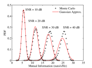
(a) $n_{t}=n_{r}=3$

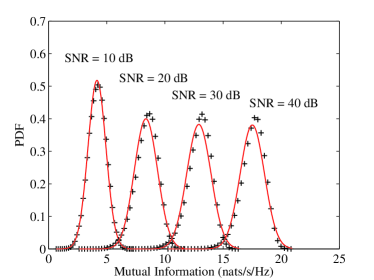
(b) $n_{t}=3,\;n_{r}=2$

Figure 1: PDF of the mutual information of MIMO Rayleigh fading channels for different antenna configurations and different SNRs.

As a second example, aside from the deviation observed in the bulk of the distribution for large SNR, it turns out that the Gaussian approximation is typically very inaccurate in the tail of the distribution when $n$ is finite and the SNR is either small or large. This is observed in Figs. 2(a)–2(b), where in both cases the Gaussian curve fails markedly in tracking the simulations for small but practical outage probabilities. This strong deviation from Gaussian was also discussed in [27], where a refined approximation was presented based on adopting an intuitive large-$n$ Coulomb fluid interpretation from statistical physics, leading to a set of coupled non-linear equations requiring numerical computation. As discussed therein, the main utility of the large deviations approach is that it allows one to capture the tail behavior in the regime of $O(n)$ deviations away from the mean, whilst the Gaussian is restricted to capturing deviations which are close to $O(1)$.

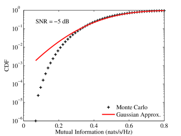
(a) $n_{t}=4,\;n_{r}=2$

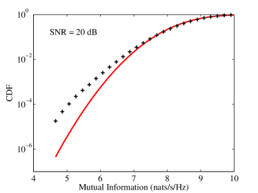
(b) $n_{t}=4,\;n_{r}=2$

Figure 2: CDF of mutual information of MIMO Rayleigh fading channels for small and large SNRs.

Obtaining a clear and rigorous understanding of the distributional behavior indicated above appears difficult with random matrix theoretic tools which are currently well known to information and communication theorists, such as those based on the Stieltjes transform [23] and the replica method [21, 26]. To address this problem, in our recent work [24] we introduced a powerful methodology involving orthogonal polynomials and their so-called “ladder operators” which led to a new and convenient exact characterization of the MGF of the mutual information in terms of a Painlevé differential equation. This valuable representation provides the machinery for systematically capturing the finite-$n$ corrections to the asymptotic Gaussian results, and thereby investigating deviations from Gaussian and correcting for them. Some related subsequent work for interference-limited multi-user MIMO systems was also presented in [28]. However, whilst the Painlevé MGF representation in [24] laid the platform for further analysis, the main focus of the analysis presented therein was restricted to the case $n_{t}=n_{r}$. Moreover, even for this case, a rigorous treatment of the large-deviations region considered in [27] was not pursued.

In this paper, we significantly expand upon our existing studies in [24] to provide a much broader characterization and understanding of the MIMO mutual information distribution. Starting with the exact Painlevé representation for the mutual information MGF derived in [24], for sufficiently large $n$ (but not assuming that $n_{t}=n_{r}$), we systematically compute new closed-form expansions for the higher order cumulants of the mutual information distribution. These series expansions reveal interesting fundamental differences between the two cases, $n_{t}\neq n_{r}$ and $n_{t}=n_{r}$. Notably, it is demonstrated that the typical approach of considering only the leading-order terms in the large-$n$ series expansions for each cumulant (e.g., (1) and (2) respectively for the mean and variance) is relatively stable for the asymmetric case $n_{t}\neq n_{r}$ compared with the symmetric case $n_{t}=n_{r}$, when the SNR $P$ becomes large. This is because the correction series for each cumulant (i.e., comprising all terms other than the leading $n$ term) is shown to converge to a bounded constant as $P$ increases, and therefore becomes quite small relative to the leading term when $P$ is large. For the symmetric case, on the other hand, the situation is very different—the correction series for each cumulant not only grows with $P$, but also at a faster rate than the leading term; a phenomenon which was discussed at length in [24]. These results allow us to provide a technical explanation for the intriguing large-SNR phenomena observed in Figs. 1(a) and 1(b).

In addition to gaining fundamental insight into the behavior of the mutual information distribution, we also provide new accurate analytical characterizations for the distribution by employing two different approaches, each being useful in their own region of interest. First, we draw upon the Edgeworth expansion technique along with our derived cumulant expressions to give a simple refined closed-form distribution approximation which is shown to be very accurate around the mean and also for certain moderate deviations into the tails. These results generalize previous Edgeworth expansions which were derived for the specific case of $n_{t}=n_{r}$ in [24]. It is shown that in contrast to the Gaussian approximation, which is only capable of successfully characterizing near $O(1)$ deviations around the mean (or the bulk) as $n$ increases, the Edgeworth expansion captures deviations of up to $O(n^{\epsilon})$, where $0<\epsilon\leq 1$. Here, $\epsilon$ is a key parameter which, as it increases, allows the approximation to capture the correct distribution further into the tails, however it also requires the addition of more cumulants to be included in the Edgeworth series, thereby increasing the complexity. In the extreme case, as $\epsilon\to 1$, all cumulants must be included; thus, the Edgeworth technique becomes unwieldy and alternative methods are required. In this scenario, in order to capture such “large deviations” into the tail, we exploit the saddle point method along with asymptotic integration tools to give further analytical representations. Very simple formulas are obtained for the cases of high and low SNR which, taken together, are shown to be very accurate over almost the entire range of SNR values. We point out that our saddle point results provide, in effect, an alternative characterization to the results proposed in [27], which also considered the “large deviations” regime, focusing on $O(n)$ deviations from the mean. Our results, however, are based on a more rigorous footing, stemming from the exact Painlevé representation for the mutual information MGF, as opposed to intuitive statistical physics analogies. Quite surprisingly, they are also found to be simpler.

As a final step, to further emphasize the utility of our results and methodology, we use our analytical framework to extract the well known diversity-multiplexing-tradeoff (DMT) formula of Zheng and Tse [29] which relates to the large deviations region in the left tail at large SNR, whilst also deriving similar results for the right tail. These results are found to be consistent with those obtained via the Coulomb fluid analogy in [27].

The rest of the paper is structured as follows. Section II describes the system model under consideration and introduces the Painlevé representation for the MGF of the mutual information, which is the key tool underpinning our analysis. Then, in Section III, we provide a systematic derivation of the mutual information cumulants to leading order in $n$, as well as finite-$n$ correction terms, giving closed-form expressions in both cases. Based on these new results, Section IV analyzes the $n$-asymptotic Gaussian approximation at large SNR, revealing fundamental differences between the two scenarios, $n_{t}=n_{r}$ and $n_{t}\neq n_{r}$. In Section V, we draw upon our cumulant expressions and the Edgeworth expansion technique to provide a refined approximation to the mutual information distribution, both around the mean and for moderate deviations into the tails. Subsequently, Section VI exploits the saddle point method and asymptotic integration tools to characterize the “large deviations” region, extracting key behavior such as the DMT. In the Appendix, correspondences are drawn between our analytical framework and the Coulomb fluid large deviations method used in [27].

II System Model

Considering a point-to-point communication system with $n_{t}$ transmit and $n_{r}$ receive antennas, under flat-fading, the linear MIMO channel model takes the form:

$${\bf y}={\bf Hx}+{\bf n}$$ (3)

where ${\bf y}\in\mathbb{C}^{n_{r}}$ and ${\bf x}\in\mathbb{C}^{n_{t}}$ denote the received and transmitted vector respectively, whilst ${\bf H}\in\mathbb{C}^{n_{r}\times n_{t}}$ represents the channel matrix, and ${\bf n}_{n_{r}\times 1}\in\mathbb{C}^{n_{r}}$ represents noise. Assuming rich scattering, ${\bf H}$ is modeled as Rayleigh fading, having IID entries $h_{i,j}\sim\mathcal{CN}(0,1)$, known to the receiver only. The noise is assumed ${\bf n}\sim\mathcal{CN}({\bf 0,I}_{n_{r}})$. The input is selected to be the ergodic-capacity-achieving input distribution ${\bf x}\sim\mathcal{CN}\left(0,\frac{P}{n_{t}}{\bf I}_{n_{t}}\right)$, where $P$ is the transmitted power constraint and also represents the SNR due to the normalized noise. For the model under consideration, the mutual information between the channel input and output is [30]:

$$\mathcal{I}\left({\bf x};{\bf y}\right)=\left\{\begin{array}[]{ll}\ln\det\left({\bf I}_{n}+\frac{P}{m}{\bf HH^{\dagger}}\right),\quad n_{t}\geq n_{r}\\[2.84526pt] \ln\det\left({\bf I}_{n}+\frac{P}{n}{\bf H^{\dagger}H}\right),\quad n_{t}<n_{r}\end{array}.\right.$$ (6)

According to (6), we can assume $n_{t}\geq n_{r}$ without loss of generality; otherwise, if $n_{t}<n_{r}$, we only need replace $P$ with $\beta P$.

Throughout the paper, we make the well known assumption that the channel exhibits block-fading, such that the fading coefficients vary independently from one coding block to another, but remain constant for the duration of each block. In this case, the outage probability becomes an important performance indicator, and the “capacity-versus-outage” tradeoff comes into play [31]. Quantifying this tradeoff requires the entire distribution of the mutual information (6). Consequently, a common approach is to investigate the MGF of $\mathcal{I}({\bf x;y})$:

$$\mathcal{M}(\lambda) :=E\left[\exp\left(\lambda\mathcal{I}(\mathbf{x;y})\right)\right]$$

$$=E_{\bf H}\left\{\left[\det\left({\bf I}_{n}+\frac{P}{m}\bf HH^{\dagger}\right)\right]^{\lambda}\right\}.$$ (7)

With this, the cumulant generating function (CGF) can be expressed as a power series about $\lambda=0$:

$$\mathcal{K}(\lambda) :=\ln\mathcal{M}(\lambda)=\sum_{\ell=1}^{\infty}\kappa_{\ell}\frac{\lambda^{\ell}}{\ell!}$$ (8)

where the coefficient $\kappa_{\ell}$ is the $\ell$-th cumulant of $\mathcal{I}(\mathbf{x;y})$.

To lay the foundation of our analysis, we first quote the following exact representation for the MGF (II) (or equivalently, the CGF) in [24]; a key result derived by the authors by drawing upon methods from random matrix theory (see e.g., [32, 33, 34]).

Proposition 1

The MGF (II) admits the following compact representation:

$${\cal M}(\lambda)=\exp\left(\int_{\infty}^{\beta/P}\frac{G_{n}(x)}{x}dx\right)\;$$ (9)

where $G_{n}(x)$ satisfies a version of the Painlevé V continuous $\sigma$–form:

$$\left(xG_{n}^{\prime\prime}\right)^{2}= n^{2}\left(xG_{n}^{\prime}+G_{n}^{\prime}\left(n+m+\lambda\right)/n-G_{n}\right)^{2}$$

$$-4\left(xG_{n}^{\prime}-G_{n}+nm\right)\left(G_{n}^{\prime 2}+\lambda nG^{\prime}_{n}\right),$$ (10)

with ^′ denoting the derivative with respect to (w.r.t.) $x$.

Whilst an explicit solution to the Painlevé V differential equation does not exist in general, we will show in the next subsection that it can be used to great effect to extract deep insight into the behavior of the mutual information distribution. In particular, we will use it to provide a systematic method for computing closed-form expressions for the leading-order and correction terms to the mean, variance, and higher order cumulants, as the numbers of antennas grow large. This will allow us to obtain more accurate characterizations than the asymptotic Gaussian approximation, which is based on only the leading order terms of the mean and variance.

III Systematic Derivation of the Mutual Information Statistics

In this section, we further elaborate upon our work in [24, Section IV] by making use of the Painlevé representation (i.e., Proposition 1) to obtain closed-form expressions for the higher order cumulants to leading order in $n$, as well as first-order correction terms, which apply for arbitrary $\beta$. Computing the mutual information distribution in terms of its cumulants enables us to obtain insights into the shape of the distribution, for example, studying its “Gaussianity”. Furthermore, by invoking an Edgeworth expansion approach, we will evaluate approximations for the outage probability in closed-form, avoiding explicit computation of the inverse MGF (i.e., an inverse Laplace Transform). A key contribution in this section is the generalization of the results in [24, Section IV] beyond the case $\beta=1$, and, based on these results, we will see that the mutual information distribution exhibits some key differences in the two scenarios, $\beta=1$ and $\beta>1$.

III-A Power Series Method: Valid for Small P

For a preliminary study, we use the power series method to seek solutions to (10). Noting that $\lim_{P\to 0}\ln\mathcal{M}(\lambda)=0$, we assume that for sufficiently small $P$, and thus sufficiently large $x$, that $G_{n}(x)$ admits an expansion of the form:

$$G_{n}(x)=\sum_{k=1}^{\infty}\frac{b_{k}}{x^{k}}\;$$ (11)

for some $b_{1},b_{2},\ldots$. Substituting this power series into (10) and solving for the $b_{k}$’s by matching the coefficients of $1/x^{k}$ on the left and right-hand sides, we write the first few $b_{k}$’s as follows:

$$b_{1}=-n^{2}\beta\lambda\;,$$

$$b_{2}=n^{3}\beta\left(\beta+1\right)\lambda-n^{2}\beta\lambda^{2}\;,$$

$$b_{3}=-n^{2}\beta\left(n^{2}\beta^{2}+3n^{2}\beta+n^{2}+1\right)\lambda+3n^{3}\beta\left(\beta+1\right)\lambda^{2}-n^{2}\beta\lambda^{3}\;,$$

$$b_{4}=\left[5n^{3}\beta\left(\beta+1\right)+n^{5}\beta\left(\beta+1\right)\left(\beta^{2}+5\beta+1\right)\right]\lambda$$

$$\qquad-\left[n^{4}\beta\left(6\beta^{2}+17\beta+6\right)+5n^{2}\beta\right]\lambda^{2}+6n^{3}\beta\left(\beta+1\right)\lambda^{3}-n^{2}\beta\lambda^{4}\;,$$

$$b_{5}=-\left[8n^{2}\beta+n^{4}\beta\left(15\beta^{2}+40\beta+15\right)+n^{6}\beta\left(\beta^{4}+10\beta^{3}+20\beta^{2}+10\beta+1\right)\right]\lambda$$

$$\qquad+\left[n^{5}\beta\left(10\beta^{3}+55\beta^{2}+55\beta+10\right)+40n^{3}\beta\left(\beta+1\right)\right]\lambda^{2}$$

$$\qquad-\left[n^{4}\beta\left(20\beta^{2}+55\beta+20\right)+15n^{2}\beta\right]\lambda^{3}+10n^{3}\beta\left(\beta+1\right)\beta\lambda^{4}-n^{2}\beta\lambda^{5}\;.$$

Introducing a rearrangement of the power series (11) according to the order of $\lambda$, we obtain an expression akin to the power series representation of the CGF (8): $G_{n}(x)=\lambda g_{1}(x)+\lambda^{2}g_{2}(x)+\lambda^{3}g_{3}(x)+\cdots$ where $g_{\ell},\ell=1,2,\ldots$ are each a power series in $1/x$, which we omit for the sake of conciseness. By using (9), the $\ell$-th cumulant $\kappa_{\ell}$ is then computed by

$$\kappa_{l}=l!\int_{\infty}^{\beta/P}\frac{g_{l}(x)}{x}{\rm d}x.$$ (12)

As a result of this procedure, here we write the first few $\kappa_{\ell}$’s, showing the leading order and first-order correction terms in $n$:

$$\mu=n\left(P-\frac{\beta+1}{2\beta}P^{2}+\frac{\beta^{2}+3\beta+1}{3\beta^{2}}P^{3}-\cdots\right)$$

$$\qquad+\frac{1}{n}\left(\frac{P^{3}}{3\beta^{2}}-\frac{5\left(\beta+1\right)}{4\beta^{3}}P^{4}+\frac{15\beta^{2}+40\beta+15}{5\beta^{4}}P^{5}-\cdots\right)+O\left(\frac{1}{n^{3}}\right),$$ (13)

$$\sigma^{2}=\left(\frac{P^{2}}{\beta}-\frac{2\left(\beta+1\right)}{\beta^{2}}P^{3}+\frac{6\beta^{2}+17\beta+6}{2\beta^{3}}P^{4}+\cdots\right)$$

$$\qquad+\frac{1}{n^{2}}\left(\frac{5P^{4}}{2\beta^{3}}-\frac{16\left(\beta+1\right)}{\beta^{4}}P^{5}+\frac{175\beta^{2}+456\beta+175}{3\beta^{5}}P^{6}-\cdots\right)+O\left(\frac{1}{n^{4}}\right),$$ (14)

$$\kappa_{3}=\frac{1}{n}\left(\frac{2P^{3}}{\beta^{2}}-\frac{9\left(\beta+1\right)}{\beta^{3}}P^{4}+\frac{24\beta^{2}+66\beta+24}{\beta^{4}}P^{5}-\cdots\right)$$

$$\qquad+\frac{1}{n^{3}}\left(\frac{18P^{5}}{\beta^{4}}-\frac{175\left(\beta+1\right)}{\beta^{5}}P^{6}+\frac{30\left(30\beta^{2}+77\beta+30\right)}{\beta^{6}}P^{7}-\cdots\right)+O\left(\frac{1}{n^{5}}\right),$$ (15)

$$\kappa_{4}=\frac{1}{n^{2}}\left(\frac{6P^{4}}{\beta^{3}}-\frac{48\left(\beta+1\right)}{\beta^{4}}P^{5}+\frac{4\left(50\beta^{2}+135\beta+50\right)}{\beta^{5}}P^{6}-\cdots\right)+O\left(\frac{1}{n^{4}}\right),$$ (16)

$$\kappa_{5}=\frac{1}{n^{3}}\left(\frac{24P^{5}}{\beta^{4}}-\frac{300\left(\beta+1\right)}{\beta^{5}}P^{6}+\frac{120\left(15\beta^{2}+40\beta+15\right)}{\beta^{6}}P^{7}-\cdots\right)+O\left(\frac{1}{n^{5}}\right)\;.$$ (17)

III-B General Method: Valid for Arbitrary P

From the power series expressions (13)–(17), we observe the following large $n$ series structure:

$$\mu=n\;C_{1,0}\phantom{C_{1,1}}+\frac{1}{n}C_{1,1}\phantom{+\frac{1}{n^{2}}C_{1,1}}+\frac{1}{n^{3}}C_{1,2}\phantom{+\frac{1}{n^{4}}C_{1,1}}+\frac{1}{n^{5}}C_{1,3}\phantom{+}\cdots$$

$$\sigma^{2}=\phantom{nC_{1,1}+}C_{2,0}\phantom{+\frac{1}{n}C_{1,1}}+\frac{1}{n^{2}}C_{2,1}\phantom{+\frac{1}{n^{3}}C_{1,1}}+\frac{1}{n^{4}}C_{2,2}\phantom{+\frac{1}{n^{5}}C_{1,1}}+\cdots$$

$$\kappa_{3}=\phantom{nC_{1,1}+C_{1,1}+\!\!\!}\frac{1}{n}C_{3,0}\phantom{+\frac{1}{n^{2}}C_{1,1}}+\frac{1}{n^{3}}C_{3,1}\phantom{+\frac{1}{n^{4}}C_{1,1}}+\frac{1}{n^{5}}C_{3,2}\phantom{+}\cdots$$

$$\kappa_{4}=\phantom{nC_{1,1}+C_{1,1}+\frac{1}{n}C_{1,1}+\!}\frac{1}{n^{2}}C_{4,0}\phantom{+\frac{1}{n^{3}}C_{1,1}\!\!}+\frac{1}{n^{4}}C_{4,1}\phantom{+\frac{1}{n^{5}}C_{1,1}}+\cdots$$

$$\;\vdots\phantom{=nC_{1,1}+C_{1,1}+\frac{1}{n}C_{1,1}+\frac{1}{n^{2}}C_{1,1}}\ddots\phantom{+\frac{1}{n^{4}}C_{1,1}+\frac{1}{n^{5}}}\ddots\phantom{+++\quad}$$ (18)

Note that $C_{i,j}$ is independent of $n$, but depends on $P$ and $\beta$. This structure gives an important general understanding of the mutual information distribution in terms of cumulants, and also paves the way for our arbitrary $P$ analysis. As seen from (III-B), as $n$ grows large with other parameters fixed, only the leading terms of the mean and variance survive, hence the mutual information distribution approaches Gaussian with increasing $n$. This agrees with previous results, see e.g., [16, 22, 23].

In the previous subsection we solved $C_{i,j}$ for small $P$. Here, we present a more general approach to compute these quantities in closed-form for arbitrary $P$. First, we establish a recursive computation for all cumulants to leading order in $n$ (i.e., generating $C_{\ell,0},\ell=1,2,\ldots$ along the leading diagonal in (III-B)). Then, employing the same machinery, we obtain a recursion for systematically computing the first-order correction terms for all cumulants, allowing us to derive closed-form expressions for $C_{\ell,1},\ell=1,2,\ldots$ along the second main diagonal in (III-B). This, in turn, allows us to capture improved accuracy for finite $n$. In addition to computing the terms along the diagonals of (III-B), we also demonstrate how our machinery based on the Painlevé MGF representation can be employed to systematically compute the horizontal power series expansion in (III-B) for a given cumulant, to arbitrary degree of accuracy. For this, we focus on the series computation of the mean by way of example, with the other cumulant series being computable in a similar way.

III-B1 Cumulants to Leading Order in $n$

Recalling the definition of the cumulants in (8) and their large-$n$ series structure in (III-B), we start by making the replacement $\lambda\to n\lambda$ and taking $n$ large, such that $G_{n}(x)$ admits

$$G_{n}(x)=n^{2}Y(x)+O\left(1\right)$$ (19)

where $Y(x)=\lambda y_{1}(x)+\lambda^{2}y_{2}(x)+\cdots$, independent of $n$. Here, $y_{\ell}(x)$ corresponds to the leading-order term (in $n$) for the $\ell$-th cumulant by the following integral:

$$C_{\ell,0}\!=\!\ell!\int_{\infty}^{\beta/P}\frac{y_{\ell}(x)}{x}{\rm d}x,\qquad\ell=1,2,\ldots$$ (20)

The remaining challenge is to compute closed-form formulas for $y_{\ell}(x)$, $\ell=1,2,\ldots$, in order to obtain the corresponding $C_{\ell,0}$. Substituting (19) for $G_{n}(x)$ into (10) (with $\lambda\to n\lambda$) and keeping only the leading-order terms in $n$ (i.e., $O(n^{6})$), we obtain the following equation involving $Y(x)$:

$$\left[\left(x+\beta+\lambda+1\right)Y^{\prime}-Y\right]^{2}=4\left(xY^{\prime}-Y+\beta\right)\left(Y^{\prime}+\lambda\right)Y^{\prime}\;.$$ (21)

Note that this equation completely characterizes all of the cumulants to leading order in $n$ (i.e., based on this, we may compute $C_{\ell,0},\ell=1,2,\ldots$ in the structure (III-B)). This can be done upon substituting $Y(x)=\lambda y_{1}(x)+\lambda^{2}y_{2}(x)+\cdots$ into (21) and matching the coefficients of $\lambda^{k}$ on the left and right-hand side. Using this approach, we systematically obtain equations involving $y_{k}(x),k=1,2,\ldots$ which are elaborated upon below.

The case $k=1$ characterizes the mean of the mutual information. In this case, we obtain the non-linear differential equation involving $y_{1}(x)$:

$$\left[x^{2}+2\left(\beta+1\right)x+\left(\beta-1\right)^{2}\right]\left(y_{1}^{\prime}\right)^{2}-2\left(x+\beta+1\right)y_{1}^{\prime}y_{1}-4\beta y_{1}^{\prime}+y_{1}^{2}=0\;,$$ (22)

which can be explicitly solved to give

$$y_{1}(x)=\frac{\sqrt{x^{2}+2\left(\beta+1\right)x+\left(\beta-1\right)^{2}}-x-\left(\beta+1\right)}{2}\;.$$ (23)

Integrating $y_{1}(x)$ via (20), we find a closed-form expression for $C_{1,0}$. With this expression, we find that $nC_{1,0}$ agrees precisely with the $n$-asymptotic mean of the mutual information (i.e., $\mu_{0}$ in (1)).

The case $k=2$ characterizes the variance of the mutual information. In this case, we obtain the non-linear differential equation involving $y_{1}(x)$ and $y_{2}(x)$:

$$\left\{-2\left[x^{2}+2\left(\beta+1\right)x+\left(\beta-1\right)^{2}\right]y_{1}^{\prime}+2\left(x+\beta+1\right)y_{1}+4\beta\right\}y_{2}^{\prime}$$

$$+2\left[\left(x+\beta+1\right)y_{1}^{\prime}-y_{1}\right]y_{2}+y_{1}^{\prime}\left\{4x\left(y_{1}^{\prime}\right)^{2}+2\left(x-\beta-1\right)y_{1}^{\prime}-4y_{1}^{\prime}y_{1}-2y_{1}\right\}=0.$$ (24)

Whilst seemingly complicated, quite remarkably, once we substitute $y_{1}(x)$ with (23), the coefficient of $y_{2}^{\prime}(x)$ vanishes, i.e.,

$$-2\left[x^{2}+2\left(\beta+1\right)x+\left(\beta-1\right)^{2}\right]y_{1}^{\prime}+2\left(x+\beta+1\right)y_{1}+4\beta=0\;,$$ (25)

and the differential equation (III-B1) collapses to a simple algebraic equation in $y_{2}(x)$. The solution is then easily obtained as:

$$y_{2}(x)=\frac{x}{2\sqrt{x^{2}+2\left(\beta+1\right)x+\left(\beta-1\right)^{2}}}-\frac{1}{2}\;\frac{x^{2}+\left(\beta+1\right)x}{x^{2}+2\left(\beta+1\right)x+\left(\beta-1\right)^{2}}\;.$$ (26)

Integrating $y_{2}(x)$ via (20), we obtain a closed-form expression for $C_{2,0}$ which is found to agree precisely with the approximation for the $n$-asymptotic variance of the mutual information (i.e., $\sigma^{2}$ in (2)).

The higher order cumulants, beyond the mean and variance, are characterized by the case $k>2$. Evaluating and investigating these cumulants is important, since it allows one to study deviations from Gaussian for finite dimensions. As we will see, these higher order cumulants may also be used to “refine” the Gaussian approximation to provide increased accuracy.

For $k>2$, $y_{k}(x)$ are found to satisfy the following recursion:

$$\sum_{i=1}^{k}y_{i}^{\prime}\left\{\left[x^{2}\!+\!2\left(\beta\!+\!1\right)x\!+\!\left(\beta\!-\!1\right)^{2}\right]y_{k-i+1}^{\prime}\!-\!2\left(x\!+\!\beta\!+\!1\right)y_{k-i+1}\right\}\!+\!\sum_{i=1}^{k}y_{i}y_{k-i+1}\!-\!4\beta y_{k}^{\prime}$$

$$=2\sum_{i=1}^{k-1}y_{i}^{\prime}\left[\sum_{j=1}^{k-i}\left(2xy_{j}^{\prime}y_{k-i-j+1}^{\prime}\!-\!2y_{j}^{\prime}y_{k-i-j+1}\right)\!+\!\left(x\!-\!\beta\!-\!1\right)y_{k-i}^{\prime}\!-\!y_{k-i}\right]\!-\!\sum_{i=1}^{k-2}y_{i}^{\prime}y_{k-i-1}^{\prime}\;$$ (27)

with initial conditions $y_{1}(x)$ and $y_{2}(x)$ given in (23) and (26) respectively. In theory, the recursive equation (III-B1) enables us to systematically compute the leading order expressions (in $n$) in closed-form for any desired number of higher order cumulants, in sequence. In its current form, however, (III-B1) appears very complicated. Fortunately, this expression can be simplified considerably by observing that the only term in (III-B1) which involves $y_{k}(x)$ (or its derivative) is:

$$\left\{\left[x^{2}+2\left(\beta+1\right)x+\left(\beta-1\right)^{2}\right]y_{1}^{\prime}-\left(x+\beta+1\right)y_{1}-2\beta\right\}y_{k}^{\prime}-\left[\left(x+\beta+1\right)y_{1}^{\prime}-y_{1}\right]y_{k}\;,$$ (28)

with all other terms involving the previously computed $y_{i}(x),i<k$. As for the variance, quite remarkably, the term (28) simplifies considerably upon noting that the coefficient of $y_{k}^{\prime}(x)$ is precisely zero, by virtue of (25). This interesting observation indicates that the computation of the higher cumulants, for $k>2$, only involves solving simple algebraic equations in $y_{k}(x)$, rather than non-linear differential equations involving $y_{k}(x)$ and $y_{k}^{\prime}(x)$. More specifically, the recursive equation (III-B1) collapses to the following:

$$y_{k}=\frac{R_{k}\!-\!\sum_{i=2}^{k-1}\left\{\left[x^{2}\!+\!2\left(\beta\!+\!1\right)x\!+\!\left(\beta\!-\!1\right)^{2}\right]y_{i}^{\prime}y_{k-i+1}^{\prime}\!-\!2\left(x+\beta+1\right)y_{i}^{\prime}y_{k-i+1}+y_{i}y_{k-i+1}\right\}}{2\left[\left(x+\beta+1\right)y_{1}^{\prime}-y_{1}\right]}$$ (29)

for $k=3,4,\ldots$, where $R_{k}$ represents the right-hand side of (III-B1), which depends only on the previously computed $y_{i}(x),i<k$. With this result, $y_{k}(x)$ can be easily computed, systematically in closed-form, for any value of $k$. We simply write down $y_{3}(x)$ and $y_{4}(x)$ here by way of example:

$$y_{3}(x)=-\frac{1}{2}\;x\left(x+1-\beta\right)\left(x-1+\beta\right)\left(\frac{x+\beta+1-\sqrt{x^{2}+2\left(\beta+1\right)x+\left(\beta-1\right)^{2}}}{\left(x^{2}+2\left(\beta+1\right)x+\left(\beta-1\right)^{2}\right)^{5/2}}\right)\;,$$ (30)

$$y_{4}(x)=\frac{x}{2}\frac{3x^{4}+\left(\beta+1\right)x^{3}-\left(\beta-1\right)^{2}\left[6x^{2}+3\left(\beta+1\right)x-\left(\beta-1\right)^{2}\right]}{\left(x^{2}+2\left(\beta+1\right)x+\left(\beta-1\right)^{2}\right)^{7/2}}$$

$$\quad+\frac{x}{2}\frac{-3x^{5}\!-\!4\left(1\!+\!\beta\right)x^{4}\!+\!\left(\beta\!-\!1\right)^{2}\left[5x^{3}\!+\!9\left(\beta\!+\!1\right)x^{2}\!+\!2\left(\beta\!+\!1\right)^{2}x\!-\!\left(\beta\!+\!1\right)\left(\beta\!-\!1\right)^{2}\right]}{\left(x^{2}+2\left(\beta+1\right)x+\left(\beta-1\right)^{2}\right)^{4}}\;.$$ (31)

Integrating $y_{k}(x)$ via (20), we obtain $C_{3,0}$ and $C_{4,0}$ in (III-B) in closed form:

$$C_{3,0}=\frac{\beta+1}{2\beta}-\frac{3\beta P}{\beta^{2}+2\left(\beta+1\right)\beta P+\left(\beta-1\right)^{2}P^{2}}$$

$$\qquad-\frac{1}{2}\frac{\left(\beta-1\right)^{2}\left[\left(\beta^{2}+1\right)P^{3}+3\beta\left(\beta+1\right)P^{2}\right]+3\beta^{2}\left(\beta^{2}+1\right)P+\beta^{3}\left(\beta+1\right)}{\beta\left(\beta^{2}+2\left(\beta+1\right)\beta P+\left(\beta-1\right)^{2}P^{2}\right)^{3/2}}\;,$$ (32)

$$C_{4,0}=-\!\frac{\beta^{2}\!+\!1}{2\beta^{2}}\!+\!\frac{18\beta^{4}\!+\!28\beta^{3}\left(\beta\!+\!1\right)P\!+\!\left(\beta\!-\!1\right)^{2}\left[3\beta^{2}P^{2}\!-\!6\beta\left(\beta\!+\!1\right)P^{3}\!+\!\left(\beta\!-\!1\right)^{2}P^{4}\right]}{\left(\beta^{2}+2\left(\beta+1\right)\beta P+\left(\beta-1\right)^{2}P^{2}\right)^{3}}P^{2}$$

$$\qquad\qquad+\frac{1}{2\beta^{2}\left(\beta^{2}+2\left(\beta+1\right)\beta P+\left(\beta-1\right)^{2}P^{2}\right)^{5/2}}\bigg{[}\left(\beta^{2}+1\right)\beta^{5}+5\beta^{4}\left(\beta+1\right)\left(\beta^{2}+1\right)P$$

$$\qquad\qquad+\left(10\beta^{4}+10\beta^{3}-16\beta^{2}+10\beta+10\right)\beta^{3}P^{2}+10\beta^{2}\left(\beta+1\right)\left(\beta^{2}+\beta+1\right)\left(\beta-1\right)^{2}P^{3}$$

$$\qquad\qquad+\beta\left(5\beta^{4}+14\beta^{2}+5\right)\left(\beta-1\right)^{2}P^{4}+\left(\beta+1\right)\left(\beta-1\right)^{6}P^{5}\bigg{]}\;.$$ (33)

As expected, expanding (32) and (33) about $P=0$ gives exactly the same power series as the leading terms in (15) and (16).

III-B2 Cumulants to Second Order in $n$

In addition to computing the cumulants to leading order in $n$, it is also of interest to compute the correction terms (in $n$), to capture deviations and achieve higher accuracy at finite $n$. To this end, similar to before, we consider

$$G_{n}(x)=n^{2}Y(x)+Z(x)+O\left(n^{-2}\right)$$ (34)

where $Y(x)$ is defined as in (19) whilst $Z(x)=\lambda z_{1}(x)+\lambda^{2}z_{2}(x)+\cdots$, independent of $n$. Here, $z_{\ell}(x)$ corresponds to the first-order correction term for the $\ell$-th cumulant (i.e., characterized by $C_{\ell,1},\ell=1,2,\ldots$ in (III-B)) by the following integral:

$$C_{\ell,1}\!=\!\ell!\int_{\infty}^{\beta/P}\frac{z_{\ell}(x)}{x}{\rm d}x,\qquad\ell=1,2,\ldots$$ (35)

Substituting (34) into (10) (with $\lambda\to n\lambda$) and setting the second leading-order terms (in $n$) to be zero, we obtain the simple algebraic equation involving $Z(x)$:

$$\Big{\{}2\beta\lambda-\left[\lambda^{2}+2(1+\beta-x)\lambda+x^{2}+2(1+\beta)x+(\beta-1)^{2}\right]Y^{\prime}+(x-\lambda+\beta+1)Y$$

$$-4Y^{\prime}Y+6xY^{\prime 2}\Big{\}}Z^{\prime}=\left(2\left(Y^{\prime}\right)^{2}-\left(x+\beta+1-\lambda\right)Y^{\prime}-Y\right)Z-\frac{x^{2}}{2}\left(Y^{\prime\prime}\right)^{2}\;.$$ (36)

This equation captures the exact first-order corrections to all leading order cumulant approximations. Substituting $Y(x)=\lambda y_{1}(x)+\lambda^{2}y_{2}(x)+\cdots$ and $Z(x)=\lambda z_{1}(x)+\lambda^{2}z_{2}(x)+\cdots$ into (III-B2) and matching the coefficients of $\lambda^{k}$, we are able compute the $z_{k}(x)$’s systematically.

The case $k=1$ corresponds to the correction term for the mean. In this case, we obtain the equation involving $z_{1}(x)$:

$$\left\{2\beta-[x^{2}+2(\beta+1)x+(\beta-1)^{2}]y_{1}^{\prime}+(x+\beta+1)y_{1}\right\}z_{1}^{\prime}$$

$$\qquad\qquad\qquad\qquad+\left[\left(x+\beta+1\right)y_{1}^{\prime}-y_{1}\right]z_{1}+\frac{x^{2}}{2}y_{1}^{\prime\prime 2}=0\;.$$ (37)

Again, once we substitute $y_{1}(x)$ with (23), the coefficient of the $z_{1}^{\prime}(x)$ vanishes and (III-B2) collapses to an algebraic equation whose solution is

$$z_{1}(x)=\frac{-\beta x^{2}}{\left(x^{2}+2\left(\beta+1\right)x+\left(\beta-1\right)^{2}\right)^{5/2}}\;.$$ (38)

The case $k=2$ corresponds to the correction term for the variance. In this case, we obtain the equation involving $z_{2}(x)$:

$$\left\{2\beta-[x^{2}+2(\beta+1)x+(\beta-1)^{2}]y_{1}^{\prime}+(x+\beta+1)y_{1}\right\}z_{2}^{\prime}+\left[(x+\beta+1)y_{1}^{\prime}-y_{1}\right]z_{2}$$

$$\!+\!\left\{2\beta\!-\![x^{2}+2(\beta+1)x\!+\!(\beta\!-\!1)^{2}]y_{2}^{\prime}\!+\!(x+\beta+1)y_{2}\!+\!6x(y_{1}^{\prime})^{2}\!-\!2(1+\beta-x)y_{1}^{\prime}\!-\!4y_{1}^{\prime}y_{1}\!-\!y_{1}\right\}z_{1}^{\prime}$$

$$+\left[(x+\beta+1)y_{1}^{\prime}-y_{1}\right]z_{1}+\left[(x+\beta+1)y_{2}^{\prime}-2(y_{1}^{\prime})^{2}-y_{2}-y_{1}^{\prime}\right]=0\;.$$ (39)

The coefficient of $z_{2}^{\prime}(x)$ is the same as in (III-B2) and vanishes, which means (III-B2) is an algebraic equation for $z_{2}(x)$. More interestingly, after substituting $y_{1}(x)$ with (23) and $y_{2}(x)$ with (III-B1), the coefficient of $z_{1}^{\prime}(x)$ also becomes zero, which further simplifies the computation. Thus we obtain $z_{2}(x)$ as follows:

$$z_{2}(x) =\frac{\left[(x+\beta+1)y_{1}^{\prime}-y_{1}\right]z_{1}+\left[(x+\beta+1)y_{2}^{\prime}-2(y_{1}^{\prime})^{2}-y_{2}-y_{1}^{\prime}\right]}{(x+\beta+1)y_{1}^{\prime}-y_{1}}$$

$$=-\frac{x^{2}}{2}\frac{\left(\beta+1\right)x^{2}+2\left(\beta^{2}-3\beta+1\right)x+\left(\beta+1\right)\left(\beta-1\right)^{2}}{\left(x^{2}+2\left(\beta+1\right)x+\left(\beta-1\right)^{2}\right)^{7/2}}$$

$$\quad+\frac{x^{2}}{2}\frac{\left(\beta\!+\!1\right)x^{3}\!+\!\left(3\beta^{2}\!-\!14\beta\!+\!3\right)x^{2}\!+\!\left(3\beta\!-\!1\right)\left(\beta\!-\!3\right)\left(\beta\!+\!1\right)x\!+\!\left(\beta^{2}\!+\!10\beta\!+\!1\right)\left(\beta\!-\!1\right)^{2}}{\left(x^{2}\!+\!2\left(\beta\!+\!1\right)x\!+\!\left(\beta\!-\!1\right)^{2}\right)^{4}}\;.$$ (40)

For the case $k>2$, we can derive a recursive equation as follows:

$$\sum_{i=1}^{k}z_{i}^{\prime}\left\{[x^{2}+2(\beta+1)x+(\beta-1)^{2}]y_{k-i+1}^{\prime}+(x+\beta+1)y_{k-i+1}\right\}+2\beta z_{k}^{\prime}$$

$$=\sum_{i=1}^{k-1}z_{i}^{\prime}\left\{y_{k-i}+2(1+\beta-x)y_{k-i}^{\prime}+4\sum_{j=1}^{k-i}y_{k-i-j+1}^{\prime}y_{j}-6x\sum_{j=1}^{k-j}y_{k-i-j+1}^{\prime}y_{j}^{\prime}\right\}+\sum_{i=1}^{k-2}z_{i}^{\prime}y_{k-i-1}^{\prime}$$

$$-\sum_{i=1}^{k}z_{i}\left[\left(x\!+\!\beta\!+\!1\right)y_{k-i+1}^{\prime}\!-\!y_{k-i+1}\right]+\sum_{i=1}^{k-1}z_{i}\left[2\sum_{j=1}^{k-i}y_{j}^{\prime}y_{k-i-j+1}^{\prime}\!+\!y_{k-i}^{\prime}\right]\!-\!\frac{x^{2}}{2}\sum_{i=1}^{k}y_{i}^{\prime\prime}y_{k-i+1}^{\prime\prime}\;.$$ (41)

The only term in (III-B2) which involves $z_{k}(x)$ (or its derivative) is:

$$\left\{-\left[x^{2}+2(\beta+1)x+(\beta-1)^{2}\right]y_{1}^{\prime}+(x+\beta+1)y_{1}+2\beta\right\}z_{k}^{\prime}+[(x+\beta+1)y_{1}^{\prime}-y_{1}]z_{k}$$ (42)

where the coefficient of $z_{k}^{\prime}(x)$ is exactly the same as the one of $y_{k}^{\prime}(x)$ in (28), which has been shown to be zero. This observation indicates that we only need to solve an algebraic equation for $z_{k}(x)$. Interestingly, apart from $z_{k}^{\prime}(x)$, it is found that the coefficients of $z_{i}^{\prime}(x),i=1,2,\dots,k-1$ in (III-B2) are also identically equal to zero.

Given that this vanishing property holds for any $k$, eliminating terms involving $z_{i}^{\prime}(x),i=1,2,\dots,k$ in (III-B2) immediately leads to the general recursive solution:

$$z_{k}=\frac{\sum_{i=1}^{k-1}z_{i}\left[2\sum_{j=1}^{k-i}y_{j}^{\prime}y_{k-i-j+1}^{\prime}\!+\!y_{k-i}^{\prime}\!-\!\left(x\!+\!\beta\!+\!1\right)y_{k-i+1}^{\prime}+y_{k-i+1}\right]\!-\!\frac{x^{2}}{2}\sum_{i=1}^{k}y_{i}^{\prime\prime}y_{k-i+1}^{\prime\prime}}{\left(x\!+\!\beta\!+\!1\right)y_{1}^{\prime}\!-\!y_{1}}\;.$$ (43)

With this result, we can compute $z_{k}(x)$ in closed-form for any value of $k$. For example, $z_{3}(x)$ is evaluated as follows:

$$z_{3}(x)=-\frac{x^{2}}{2\left(x^{2}+2\left(\beta+1\right)x+\left(\beta-1\right)^{2}\right)^{6}}\Bigg{[}-x^{7}+8\left(\beta+1\right)x^{6}+\left(49\beta^{2}-38\beta+49\right)x^{5}$$

$$+6\left(\beta+1\right)\left(15\beta^{2}-38\beta+15\right)x^{4}+\left(65\beta^{4}-76\beta^{3}-42\beta^{2}-76\beta+65\right)x^{3}$$

$$+4\left(\beta+1\right)\left(\beta^{2}+26\beta+1\right)\left(\beta-1\right)^{2}x^{2}-\left(17\beta^{2}-46\beta+17\right)\left(\beta-1\right)^{4}x-6\left(\beta+1\right)\left(\beta-1\right)^{6}\Bigg{]}$$

$$-\frac{x^{2}}{2\left(x^{2}+2\left(\beta+1\right)x+\left(\beta-1\right)^{2}\right)^{11/2}}\Bigg{[}x^{6}-9\left(\beta+1\right)x^{5}-8\left(5\beta^{2}-11\beta+5\right)x^{4}$$

$$-10\left(\beta+1\right)\left(5\beta^{2}-13\beta+5\right)x^{3}-\left(15\beta^{4}+134\beta^{3}-330\beta^{2}+134\beta+15\right)x^{2}$$

$$+\left(\beta+1\right)\left(11\beta^{2}-100\beta+11\right)\left(\beta-1\right)^{2}x+6\left(\beta^{2}+5\beta+1\right)\left(\beta-1\right)^{4}\Bigg{]}.$$ (44)

Integrating $z_{k}(x)$ via (35), we obtain the first-order correction terms in closed-form. For example, $C_{1,1}$ and $C_{2,1}$ are given as follows:

$$C_{1,1}=-\frac{\beta\!+\!1}{24\beta}\!+\!\frac{\beta^{3}\left(\beta\!+\!1\right)\!+\!3\beta^{2}\left(\beta\!+\!1\right)^{2}P\!+\!3\beta\left(\beta\!+\!1\right)\left(\beta^{2}\!+\!1\right)P^{2}\!+\!\left(\beta^{2}\!+\!1\right)\left(\beta\!-\!1\right)^{2}P^{3}}{24\beta\left(\beta^{2}+2\beta\left(\beta+1\right)P+\left(\beta-1\right)^{2}P^{2}\right)^{3/2}}\;,$$ (45)

$$C_{2,1}=\frac{\beta^{2}\!+\!1}{24\beta^{2}}\!-\!\frac{4\left(\beta\!+\!1\right)\beta^{3}P^{3}\!+\!\left(9\beta^{2}\!-\!42\beta\!+\!9\right)\beta^{2}P^{4}\!+\!6\beta\left(\beta\!+\!1\right)\left(\beta\!-\!1\right)^{2}P^{5}\!+\!\left(\beta\!-\!1\right)^{4}P^{6}}{12\left(\beta^{2}+2\beta\left(\beta+1\right)P+\left(\beta-1\right)^{2}P^{2}\right)^{3}}$$

$$-\frac{1}{24\beta^{2}\left(\beta^{2}+2\beta\left(\beta+1\right)P+\left(\beta-1\right)^{2}P^{2}\right)^{7/2}}\Bigg{[}\left(\beta^{2}+1\right)\beta^{7}+7\beta^{6}\left(\beta+1\right)\left(\beta^{2}+1\right)P$$

$$+7\beta^{5}\left(\beta^{2}+1\right)\left(3\beta^{2}+4\beta+3\right)P^{2}+\left(\beta+1\right)\left(35\beta^{4}+62\beta^{2}+35\right)\beta^{4}P^{3}$$

$$+\left(35\beta^{6}\!+\!9\beta^{4}\!+\!8\beta^{3}\!+\!9\beta^{2}\!+\!35\right)\beta^{3}P^{4}\!+\!\left(\beta\!+\!1\right)\left(\beta\!-\!1\right)^{2}\left(21\beta^{4}\!-\!14\beta^{3}\!-\!2\beta^{2}\!-\!14\beta\!+\!21\right)\beta^{2}P^{5}$$

$$+7\left(\beta+1\right)^{2}\left(\beta-1\right)^{6}\beta P^{6}+\left(\beta+1\right)\left(\beta-1\right)^{8}P^{7}\Bigg{]}.$$ (46)

The first-order correction terms to the higher cumulants $\kappa_{3},\kappa_{4},\ldots$ are omitted here in order to keep the presentation concise, though they follow trivially. Again, expanding (45) and (46) about $P=0$ yields exactly the same power series as the $O(n^{-1})$ term in (13) and the $O(n^{-2})$ term in (46). Note that if we aim to compute further high order correction terms (i.e., $C_{i,j},i=1,2,\ldots,j\geq 2$) for each cumulant, we can invoke the same procedure as what has been used for computing the two leading-order terms, which only takes more algebraic effort.

III-B3 Large-$n$ Series Computation for a Given Cumulant

In addition to the machinery used in the previous subsection for systematically computing the high order cumulants one after the other for a given order in $n$, we can also derive recursions for systematically computing the large-$n$ series for a given cumulant. Here we give the computation of the mean as an example, with the corresponding computations for the higher cumulants following similarly. More details for the specific case $n_{t}=n_{r}$ can be found in [24].

Based on the power series representation of the CGF (in $\lambda$), substituting

$$G_{n}(x)=\lambda g_{1}(x)+\lambda^{2}g_{2}(x)+\lambda^{3}g_{3}(x)+\cdots$$ (47)

into (10) and matching the coefficients of $\lambda^{k}$, we obtain the equations for $g_{i}(x),i=1,2,\ldots$. For the mean we are interested in $g_{1}(x)$, which takes the form:

$$x^{2}\left(g_{1}^{\prime\prime}\right)^{2}- n^{2}\left(x^{2}+2\left(\beta+1\right)x+\left(\beta-1\right)^{2}\right)\left(g_{1}^{\prime}\right)^{2}$$

$$+2n^{2}\left[\left(x+\beta+1\right)g_{1}+2\beta n\right]g_{1}^{\prime}-n^{2}g_{1}^{2}=0\;.$$ (48)

Making use of the large-$n$ series structure in (III-B), we assume

$$g_{1}(x)=nQ_{0}(x)+\frac{1}{n}Q_{1}(x)+\frac{1}{n^{3}}Q_{2}(x)+\ldots$$ (49)

where $Q_{\ell}(x),\ell=0,1,\ldots$ are independent of $n$ and are related to the large-$n$ series expansion for the mean via the following integral:

$$C_{1,\ell}=\int_{\infty}^{\beta/P}\frac{Q_{\ell}(x)}{x}{\rm d}x,\qquad\ell=1,2,\ldots$$ (50)

Substituting (49) into (III-B3) and matching the coefficients of $n^{k}$, equations involving $Q_{\ell}(x),\ell=0,1,\ldots$ are obtained successively. Considering the highest order in $n$, we have

$$\left[x^{2}+2\left(\beta+1\right)+\left(\beta-1\right)^{2}\right]\left(Q_{0}^{\prime}\right)^{2}-2\left[\left(x+\beta+1\right)Q_{1}+2\beta\right]Q_{0}^{\prime}+Q_{0}^{2}=0\;.$$ (51)

Note that this equation is exactly the same as (22), because they both characterize the leading order term (in $n$) of the mean and lead to the same solution (23). For $k\geq 1$, we derive the following recursion

$$4\beta Q_{k}^{\prime}+2(x+\beta+1)\sum_{i=0}^{k}Q_{k-i}Q_{i}^{\prime}+x^{2}\sum_{i=0}^{k-1}Q_{k-i-1}^{\prime\prime}Q_{i}^{\prime\prime}$$

$$=\sum_{i=0}^{k}Q_{k-i}Q_{i}+\sum_{i=0}^{k}\left[x^{2}+2(\beta+1)x+(\beta-1)^{2}\right]Q_{k-i}^{\prime}Q_{i}^{\prime}.$$ (52)

Interestingly enough, we find again that in (III-B3), the only term which involves $Q_{k}(x)$ (or its derivative) is

$$\left\{-2\left[x^{2}+2(\beta+1)x+(\beta-1)^{2}\right]Q_{0}^{\prime}+2(x+\beta+1)Q_{0}+4\beta\right\}Q_{k}^{\prime}+2\left[(x+\beta+1)Q_{0}^{\prime}-Q_{0}\right]Q_{k}$$

where the coefficient of $Q_{k}^{\prime}(x),k=1,2,\ldots$ vanishes identically. Setting $k=1$ results in exactly the same equation as (III-B2), since they both correspond to $C_{1,1}$ in (III-B). For $k\geq 2$ we obtain the general recursion of $Q_{k}(x)$:

$$Q_{k}=$$

$$\frac{\sum_{i=1}^{k-1}\!\left[Q_{k-i}Q_{i}\!+\!\left(x^{2}\!+\!2(\beta\!+\!1)x\!+\!(\beta\!-\!1)^{2}\right)Q_{k-i}^{\prime}Q_{i}^{\prime}\!-\!2(x\!+\!\beta\!+\!1)Q_{k-i}Q_{i}^{\prime}\right]\!-\!x^{2}\!\sum_{i=0}^{k-1}\!Q_{k-i-1}^{\prime\prime}Q_{i}^{\prime\prime}}{2\left[(x+\beta+1)Q_{0}^{\prime}-Q_{0}\right]}.$$ (53)

Note that this recursion is a generalization of [24, Eq. (132)] which was derived for $\beta=1$. Integrating $Q_{k}(x)$ via (50) gives us closed-form expressions for $C_{1,\ell},\ell=0,1,\ldots$. We write $C_{1,2}$ here as an example, and omit the presentation of the higher order correction formulas for the sake of conciseness:

$$C_{1,2}=\frac{1+\beta^{3}}{240\beta^{3}}-\frac{1}{240\beta^{3}\left((\beta-1)^{2}P^{2}+2(\beta+1)P+\beta^{2}\right)^{9/2}}\Big{[}\left(1+{\beta}^{3}\right){\beta}^{9}+9\left({\beta}^{2}-\beta+1\right)\left(\beta+1\right)^{2}{\beta}^{8}P$$

$$+18\left(\beta+1\right)\left(2{\beta}^{2}+3\beta+2\right)\left({\beta}^{2}-\beta+1\right){\beta}^{7}{P}^{2}+42\,\left(2{\beta}^{2}+\beta+2\right)\left({\beta}^{2}-\beta+1\right)\left(\beta+1\right)^{2}{\beta}^{6}{P}^{3}$$

$$+42\left(2{\beta}^{2}+\beta+2\right)\left({\beta}^{2}-\beta+1\right)\left(\beta+1\right)^{2}{\beta}^{5}{P}^{4}+\left(126+126{\beta}^{8}-384{\beta}^{4}+126{\beta}^{5}+126{\beta}^{3}\right){\beta}^{4}{P}^{5}$$

$$+6\left(\beta+1\right)\left(14{\beta}^{8}-35{\beta}^{7}+35{\beta}^{6}-21{\beta}^{5}-16{\beta}^{4}-21{\beta}^{3}+35{\beta}^{2}-35\beta+14\right){\beta}^{3}{P}^{6}$$

$$+6\left(6{\beta}^{8}-9{\beta}^{7}-3{\beta}^{6}+9{\beta}^{5}+56{\beta}^{4}+9{\beta}^{3}-3{\beta}^{2}-9\beta+6\right)\left(\beta-1\right)^{2}{\beta}^{2}{P}^{7}$$

$$+9\left(\beta+1\right)\left({\beta}^{6}-3{\beta}^{5}+3{\beta}^{4}+3\,{\beta}^{2}-3\beta+1\right)\left(\beta-1\right)^{4}\beta\,{P}^{8}+\left({\beta}^{6}-3{\beta}^{5}+3{\beta}^{4}+3{\beta}^{2}-3\beta+1\right)\left(\beta-1\right)^{6}{P}^{9}\Big{]}.$$ (54)

Systematic derivations of the series expansions for the variance and higher order cumulants follow similarly, using the same approach. In this way, one can obtain the large-$n$ series for each cumulant to arbitrary degree of accuracy.

IV Large SNR Analysis of the Gaussian Deviation

The systematic high order cumulant expansions derived in the previous section allow us to closely investigate the behavior of the mutual information distribution under various conditions. For example, our analysis in Section III-B1 recovered the fact that as the number of antennas $n$ grows large, with the SNR $P$ kept fixed, the distribution approaches a Gaussian. However, in practice, the number of antennas is finite and is not typically huge (though some recent trends have considered such systems [35, 36, 37, 38, 39]), whilst the SNR may vary significantly depending on the application. Thus, a natural question is, for asymptotically high SNR, if and by how much the mutual information distribution deviates from Gaussian.

In this section, we focus on the high SNR regime of the mutual information. In this case, as shown in Figs. 1(a)–1(b), the distribution appears to deviate from Gaussian as the SNR becomes large, whilst the deviation appears to be much stronger for the case of equal numbers of transmit and receive antennas (i.e., $n=m$) compared with the case $n\neq m$. This is an interesting observation which thus far has resisted theoretical validation or explanation. Here we draw insight into this phenomenon by employing our new closed-form high order cumulant expansions given in the previous section.

Interestingly, by taking $P$ large in (1), (2), (32), (45) and (46), it turns out that we obtain very different limiting results depending on whether $\beta=1$ (i.e., $n_{t}=n_{r}$) or not. For $\beta=1$, as $P$ grows large we obtain:

$$\mu\sim n\ln P+\frac{1}{16}\frac{\sqrt{P}}{n}+\frac{3}{1024}\left(\frac{\sqrt{P}}{n}\right)^{3}+\frac{45}{32768}\left(\frac{\sqrt{P}}{n}\right)^{5}+\cdots\;$$ (55)

$$\sigma^{2}\sim\frac{1}{2}\ln\left(\frac{P}{2}\right)+\frac{1}{32}\left(\frac{\sqrt{P}}{n}\right)^{2}+\cdots\;$$ (56)

$$\kappa_{3}\sim\frac{1}{4n}+\frac{1}{32}\left(\frac{\sqrt{P}}{n}\right)^{3}+\cdots$$ (57)

These large-$n$—large-$P$ series expansions were also documented in [24], which focused primarily on the case $n_{t}=n_{r}$. From these expressions, we see that for each cumulant the correction terms grow with $P$, and indeed grow faster than the leading order terms. As such, approximating each cumulant via their leading order term will be inaccurate when $P$ is large.

Now, considering $\beta\neq 1$, we obtain:

$$\mu\sim n\left[\ln P-\left(\beta-1\right)\ln\left(\frac{\beta-1}{\beta}\right)-1\right]+\frac{1}{n}\left[\frac{1}{12\left(\beta-1\right)}-\frac{1}{12\beta}\right]$$

$$\qquad+\frac{1}{n^{3}}\left[-\frac{1}{120(\beta-1)^{3}}+\frac{1}{120\beta^{3}}\right]+\frac{1}{n^{5}}\left[-\frac{1}{252(\beta-1)^{5}}+\frac{1}{252\beta^{5}}\right]+\cdots\;,$$ (58)

$$\sigma^{2}\sim\ln\left(\frac{\beta}{\beta-1}\right)+\frac{1}{n^{2}}\left[-\frac{1}{12\left(\beta-1\right)^{2}}+\frac{1}{12\beta^{2}}\right]+\cdots\;,$$ (59)

$$\kappa_{3}\sim\frac{1}{n}\left[-\frac{1}{\left(\beta-1\right)}+\frac{1}{\beta}\right]+\frac{1}{n^{3}}\left[\frac{1}{6\left(\beta-1\right)^{3}}-\frac{1}{6\beta^{3}}\right]+\cdots\;\;.$$ (60)

From these we can make some key observations, which we summarize in the following remarks:

Remark 1

In contrast to the results in (55)–(57), for $n_{t}\neq n_{r}$, all terms other than the leading term of $\mu$ are strictly bounded as $P$ increases, converging to constants depending on $\beta$. Moreover, as $n$ or $\beta$ increase, the correction terms have less effect, eventually becoming negligible, even when $P$ is very large.

Remark 2

For $n_{t}\neq n_{r}$, the $n$-asymptotic power series representations for the cumulants remain valid for arbitrary SNR $P$; whilst in contrast, for $n_{t}=n_{r}$ they break down for sufficiently large $P$. This clearly indicates that the commonly-assumed Gaussian approximation (based on the leading order terms of $\mu$ and $\sigma$ only) is quite robust at high SNRs for the case $n_{t}\neq n_{r}$, but not for the case $n_{t}=n_{r}$.

These remarks are illustrated in Figs. 3(a)–3(c), showing $\sigma^{2}$ and $\kappa_{3}$. Fig. 3(a) shows that when $n_{t}=n_{r}$, the leading order term of $\sigma^{2}$ (i.e., representing the variance of the Gaussian approximation) and the leading order term of $\kappa_{3}$ both deviate strongly from simulations when $P$ is sufficiently large. In contrast, when $n_{t}\neq n_{r}$ (i.e., Figs. 3(b)–3(c)), the leading order cumulants capture the simulations accurately for arbitrary $P$, even with smaller $n$. We also see that increasing $\beta$ enhances the accuracy of the leading order results, whilst including the first-order correction term provides improved accuracy as well. These observations explain technically why the Gaussian approximation, based purely on the leading order terms of $\mu$ and $\sigma^{2}$, is relatively more robust to increasing SNRs in Fig. 1(b), compared with the results in Fig. 1(a). Nevertheless, even in the former case, the higher cumulants (e.g., of order $O(1/n)$) still contribute to some deviations from Gaussian. These deviations become particularly significant in the tail region, yielding the Gaussian approximation unsuitable for capturing low outage probabilities of practical interest. This will be considered further in the subsequent sections, where we will make use of our closed-form cumulant expansions to “correct” for these deviations, both in the tail and around the mean, and thereby refine the Gaussian approximation.

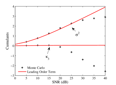
(a) $n_{t}=4,n_{r}=4$

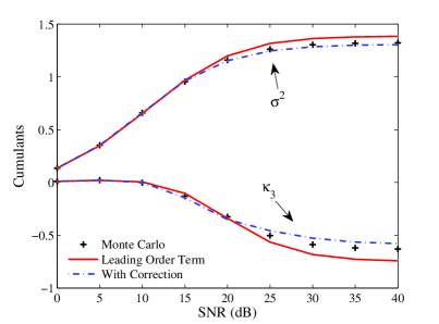
(b) $n_{t}=4,n_{r}=3$

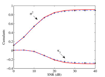
(c) $n_{t}=5,n_{r}=3$

Figure 3: Comparison of $\sigma^{2}$ to leading order (in $n$) and with first-order correction, $\kappa_{3}$ to leading order and with first-order correction, and Monte Carlo simulations. Results are shown for different antenna configurations.

Before presenting these refinements, we would like to briefly connect our large-$n$–large-$P$ cumulant expansions with existing results, which were obtained via different means by considering $n$ fixed and taking $P$ large at the beginning. This approach was used to obtain the leading-order terms of $\mu$ and $\sigma^{2}$ in [22], and these results coincide exactly with the leading-order terms in (55) and (56). In addition, the first few terms of the mean and variance expansions (i.e., (58) and (59) respectively) match exactly with the results in [40, Eq. (134)] and [41, Lemma A.2]. For example, [40] has the large-$P$ mean representation:

$$\mu \sim n\ln\left(\frac{P}{m}\right)-n+m\psi(m)-(m-n)\psi(m-n),\quad P\to\infty\;$$ (61)

which gives (58) by expanding the digamma function $\psi(x)$ at large $x$ as

$$\psi(x)=\ln{x}-\frac{1}{2x}-\frac{1}{12x^{2}}+\frac{1}{120x^{4}}-\frac{1}{252x^{6}}+O\left(\frac{1}{x^{8}}\right),\quad x\to\infty.$$ (62)

Our results can also be shown to be consistent with the large-$P$ MGF representation derived in [18].

V Characterization with the Edgeworth Expansion

Armed with closed-form expressions for $C_{i,j}$ in (III-B), in this section we draw upon the Edgeworth expansion technique. This approach allows us to start with a Gaussian distribution and to systematically correct this by including higher cumulant effects (i.e., other than the mean and variance), giving an explicit expression for the corrected PDF. Moreover, the CDF, which directly defines the outage probability, can be obtained explicitly through a straightforward integration.

We first write the MGF in the following form

$$\mathcal{M}(\lambda)=\exp\left(\sum_{\ell=3}^{\infty}\frac{\kappa_{\ell}}{\ell!}\lambda^{\ell}\right)\mathcal{M}^{(G)}(\lambda)$$ (63)

where $\mathcal{M}^{(G)}(\lambda)$ represents the MGF of a Gaussian distribution with mean $\mu$ and variance $\sigma^{2}$. Note that the MGF is, in effect, the Laplace transform of a PDF (evaluated along the real axis), thus in the PDF domain (63) is equivalent to

$$p_{\mathcal{I}(\mathbf{x};\mathbf{y})}(t)=\exp\left(\sum_{\ell=3}^{\infty}\frac{\kappa_{\ell}}{\ell!}\left(-\partial_{t}\right)^{\ell}\right)p_{\mathcal{I}(\mathbf{x};\mathbf{y})}^{(G)}(t)$$ (64)

where $p_{\mathcal{I}(\mathbf{x};\mathbf{y})}^{(G)}(t)=\frac{1}{\sqrt{2\pi}\sigma}e^{-z^{2}/2},\;z:=(t-\mu)/\sigma$ and $\partial_{t}:={\rm d}/{\rm d}t$. Expanding the exponent in (64) and collecting terms according to the powers of $\sigma$, the PDF of the mutual information takes the form [42, Eq.43]:

$$p_{\mathcal{I}(\mathbf{x};\mathbf{y})}(t)\approx\frac{1}{{\sqrt{2\pi}\sigma}}{\rm e}^{-z^{2}/2}\left[1+\mathcal{D}(z)\right]$$ (65)

where

$$\mathcal{D}(z)=\sum_{s=1}^{L}\sum_{\{k\}}\frac{{\rm He}_{s+2r}\left(z\right)}{\sigma^{s+2r}}\prod_{\ell=1}^{s}\frac{1}{k_{\ell}!}\left(\frac{\kappa_{\ell+2}}{(\ell+2)!}\right)^{k_{\ell}}$$ (66)

is the quantity which determines any deviation from Gaussian. Here, $L$ is a positive integer characterizing how many cumulants are included in the corrected PDF (i.e., $\kappa_{\ell},\ell=3,4,\ldots,L+2$ are involved). Note that the second summation enumerates all sets $k=\{k_{1},k_{2},\cdots,k_{s}\}$ containing the non-negative integer solutions of the Diophantine equation $k_{1}+2k_{2}+\cdots+sk_{s}=s$. For each of these solutions, a corresponding constant $r$ is defined as $r=k_{1}+k_{2}+\cdots+k_{s}$. In [42], a practical algorithm for computing the $\{k\}$ solutions is proposed in general. ${\rm He}_{\ell}(z)$ is the $\ell$-th Chebyshev-Hermite polynomial, with the explicit form [42, Eq. (13)]

$${\rm He}_{\ell}(z)=\ell!\sum_{k=0}^{\lfloor\ell/2\rfloor}\frac{(-1)^{k}z^{\ell-2k}}{k!(\ell-2k)!2^{k}}\;$$ (67)

where $\lfloor\cdot\rfloor$ denotes the floor function. These are generated by differentiating the standard normal distribution:

$${\rm He}_{\ell}\left(z\right)=\left(-1\right)^{\ell}g_{0}^{\left(\ell\right)}(z)/g_{0}(z)$$ (68)

where $g_{0}(z)=\exp\left(-z^{2}/2\right)/\sqrt{2\pi}$ and the superscript $(\ell)$ denotes the $\ell$-th derivative w.r.t. $z$. Here we list some specific polynomials that we are going to use subsequently:

$${\rm He}_{3}(z)=z^{3}-3z,\quad{\rm He}_{4}(z)=z^{4}-6z^{2}+3,\quad{\rm He}_{6}(z)=z^{6}-15z^{4}+45z^{2}-15\;.$$ (69)

In theory, we can approximate the mutual information distribution with arbitrary accuracy, by taking $L$ sufficiently large in $\mathcal{D}(z)$. We first set $L=2$ (i.e., including $\kappa_{3}$ and $\kappa_{4}$):

$$p_{\mathcal{I}(\mathbf{x};\mathbf{y})}(t)\approx\frac{p_{I(\mathbf{x},\mathbf{y})}^{(G)}(t)}{\sigma}\biggl{[}1+\frac{\kappa_{3}}{6\sigma^{3}}{\rm He}_{3}\left(z\right)+\frac{\kappa_{4}}{24\sigma^{4}}{\rm He}_{4}\left(z\right)+\frac{\kappa_{3}^{2}}{72\sigma^{6}}{\rm He}_{6}\left(z\right)\biggr{]}$$ (70)

and compare the Edgeworth expansion with the Monte Carlo simulations and the Gaussian approximation in Fig. 4. Note that for the Edgeworth expansion curves we only use the leading order terms of the cumulants (i.e., $C_{\ell,0}/n^{2-\ell}$ in (III-B)), since as we have shown, the leading order terms of the first few cumulants give valid approximations for arbitrary $P$ if $\beta\neq 1$ (c.f. Remark 2).

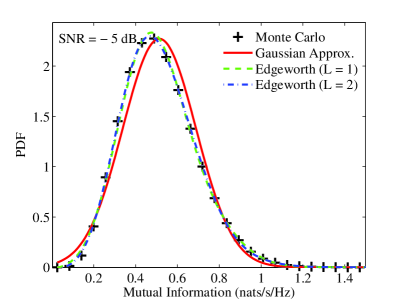
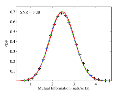
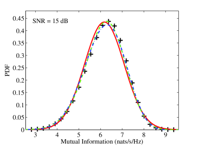
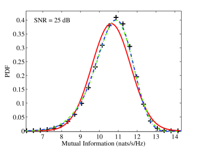
Figure 4: PDF of mutual information, comparing the Gaussian approximation, Edgeworth expansions (with $L=1$ and $L=2$), and Monte Carlo simulations. Results are shown for $n_{t}=3,n_{r}=2$ and for different SNRs.

To examine the outage probability, we need to derive the CDF of the mutual information. Recalling (68), we have

$$\int_{-\mu/\sigma}^{z}{\rm He}_{\ell}\left(u\right)g_{0}\left(u\right){\rm d}u\approx\int_{-\infty}^{z}{\rm He}_{\ell}\left(u\right)g_{0}\left(u\right){\rm d}u =-{\rm He}_{\ell-1}(z)g_{0}(z).$$ (71)

Therefore, the Edgeworth PDF formula (65) can be immediately integrated to give the CDF:

$$F_{\mathcal{I}(\mathbf{x};\mathbf{y})}(t)\approx 1-Q\left(z\right)-g_{0}(z)\sum_{s=1}^{L}\sum_{\{k\}}\frac{{\rm He}_{s+2r-1}\left(z\right)}{\sigma^{s+2r}}\prod_{\ell=1}^{s}\frac{1}{k_{\ell}!}\left(\frac{\kappa_{\ell+2}}{(\ell+2)!}\right)^{k_{\ell}}$$ (72)

where $Q(z):=\frac{1}{\sqrt{2\pi}}\int^{\infty}_{z}e^{-u^{2}/2}{\rm d}u$. Comparisons between the CDF curves computed by the Edgeworth expansion and the Gaussian approximation are made in Fig. 5. We see that in the tail region, the Edgeworth expansions with higher cumulants nicely approach the simulations (in this case, $L=6$ was required to achieve good accuracy), whilst the Gaussian curve strongly deviates. This confirms that, by the virtue of our new cumulant expressions and the Edgeworth expansion, we can compute the outage probability of MIMO systems with high accuracy in closed-form for arbitrary SNR.

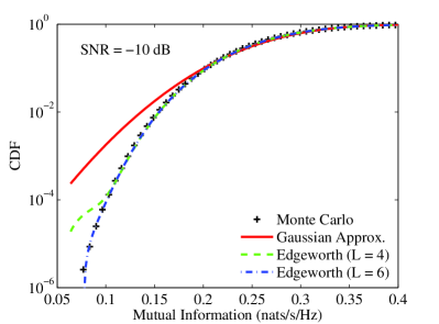
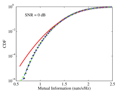
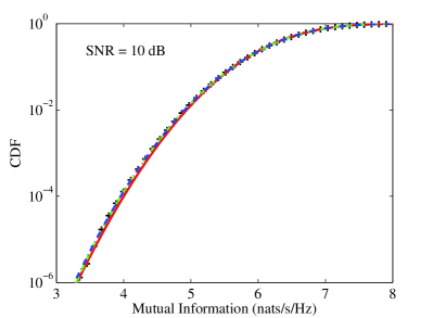
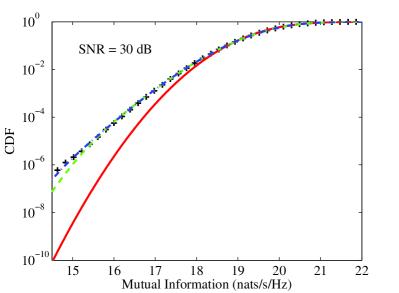
Figure 5: CDF of mutual information, comparing the Gaussian approximation, Edgeworth expansions (with $L=4$ and $L=6$), and Monte Carlo simulations. Results are shown for $n_{t}=6,n_{r}=3$ and for different SNRs.

Moreover, from these numerical tests, for small SNR (i.e., ${\rm SNR}=-10\,{\rm dB},0\,{\rm dB}$), we see that the Gaussian approximation overestimates the outage probability in the tail, whilst for large SNR, the outage probability is underestimated. These tail deviations can be analyzed as follows. For points far away from the mean (i.e., large $z$), we approximate

$${\rm He}_{\ell}\left(z\right)\sim z^{\ell},$$ (73)

and the Edgeworth expansion (66) becomes

$$\mathcal{D}(z) \approx\sum_{s=1}^{L}\sum_{\{k\}}\left(\frac{z}{\sigma}\right)^{s+2r}\prod_{\ell=1}^{s}\frac{1}{k_{\ell}!}\left(\frac{\kappa_{\ell+2}}{(\ell+2)!}\right)^{k_{\ell}}.$$ (74)

For large $z$, the highest order of $(z/\sigma)^{s+2r}$ will dominate the lower order terms. Since $r$ is maximized for $r=s$ with $\{k_{1},k_{2},\cdots,k_{s}\}=\{s,0,\cdots,0\}$, letting $L\to\infty$, $\mathcal{D}(z)$ can be further estimated as

$$\mathcal{D}(z) \approx\sum_{s=1}^{\infty}\frac{1}{s!}\left(\frac{\kappa_{3}}{6\sigma^{3}}\;z^{3}\right)^{s}$$

$$=\exp\left(\frac{\kappa_{3}}{6\sigma^{3}}\;z^{3}\right)-1\;.$$ (75)

With this, the PDF of the mutual information becomes:

$$p_{\mathcal{I}(\mathbf{x};\mathbf{y})}(t)\approx\frac{1}{{\sqrt{2\pi}\sigma}}e^{-\frac{\left(t-\mu\right)^{2}}{2\sigma^{2}}+\frac{\kappa_{3}}{6\sigma^{6}}\left(t-\mu\right)^{3}}$$ (76)

which gives a more accurate distribution than the Gaussian in the tails for finite $n$, since the effect of $\kappa_{3}$ is considered. The same formula was presented in [24], which focused on the case $n_{t}=n_{r}$. Here, we provide more general insights with our new cumulant expressions which apply for both $n_{t}=n_{r}$ and $n_{t}\neq n_{r}$.

First, (76) indicates that the Gaussian approximation is accurate under the condition:

$$|t-\mu|<<\sqrt[3]{\left|\frac{6\sigma^{6}}{\kappa_{3}}\right|}\approx\sqrt[3]{\left|\frac{6\sigma_{0}^{6}}{C_{3,0}}\right|}\;n^{1/3}\;.$$ (77)

Thus, the large-$n$ Gaussian approximation is valid for deviations of $|t-\mu|\sim O(n^{1/3})$ or less from the mean. Outside this regime, the second term of the exponent in (76) becomes non-negligible. In this case, by examining the factor $\kappa_{3}/\sigma^{6}$ in (76), we can further understand how the distribution behaves compared with the Gaussian approximation. To this end, considering the variance and third cumulant to leading order in $n$ (i.e., $\sigma_{0}^{2}$ given in (2), and $C_{3,0}/n$ with $C_{3,0}$ given in (32)), for small $P$,

$$\frac{\kappa_{3}}{\sigma^{6}}\approx\frac{2\beta}{n\,P^{3}}\;,\qquad P\to 0\;,$$ (78)

whilst for large $P$,

$$\frac{\kappa_{3}}{\sigma^{6}}\approx\left\{\begin{array}[]{ll}\frac{2}{n\,\left(\ln P\right)^{3}}\;,&\beta=1\\ \frac{1}{n\,\beta\left(\beta-1\right)\left(\ln\left(1-\beta^{-1}\right)\right)^{3}}\;,&\beta>1\end{array}\right.\;,\qquad P\to\infty\;.$$ (81)

These results are in perfect agreement with [27, Eq. (70)] obtained via Coulomb fluid arguments, and also [24, Eq. (218)] obtained for the special case $\beta=1$. Therefore, seen from (76), for small SNR, $\kappa_{3}/\sigma^{6}>0$, and the left tail of the PDF should be always above the Gaussian approximation (similarly for the CDF in the left tail). For large SNR and $\beta>1$ on the other hand, $\kappa_{3}/\sigma^{6}<0$, and the situation is the opposite.

Note that the interpretation of the large SNR results above for the particular case $\beta=1$ should be taken with caution since, as discussed in Section IV and also in [24], the leading order expressions for $\sigma^{2}$ and $\kappa_{3}$ (upon which the arguments are based) become inaccurate in that scenario, unless $n$ is also very large. For the case $\beta\neq 1$ however, there is no such problem.

VI Refining the Tail Distribution via the Saddle Point Method

Whilst the Edgeworth expansion technique provides an accurate closed-form characterization of the mutual information distribution, it becomes unwieldy when too many cumulants are needed for obtaining the desired accuracy. Particularly, in the case when one is interested in the tail region of $O(n)$ away from the mean (i.e., the “large deviation” region discussed in [27]), we need to consider the effect of all cumulants to obtain high accuracy. Therefore, to supplement the Edgeworth expansion results, in this section we will draw upon the saddle point method and the cumulant results from Section III to further investigate the large deviation scenario.

VI-A Saddle Point Method

Assuming that the MGF (equivalently, the CGF) is known, the PDF of the mutual information can be derived through the inversion formula:

$$p_{\bf\mathcal{I}(x;y)}(t)=\frac{1}{2\pi i}\int_{\tau-i\infty}^{\tau+i\infty}e^{\mathcal{K}(\lambda)-\lambda t}{\rm d}\lambda,$$ (82)

where $\mathcal{K}(\lambda)$ is the CGF and $\tau$ is a real number defining the integration path. In most cases, it is infeasible to evaluate (82) in closed-form. However, noting that $\mathcal{K}(\lambda)-\lambda t\sim O(n)$ (given $\mu\sim O(n)$, thus $\mathcal{K}(\lambda)=\mu\lambda+\frac{\sigma^{2}}{2}\lambda^{2}+\cdots\sim O(n)$ and $t=\mu+O(n)\sigma\sim O(n)$), if $n$ is large, the saddle point method in [43] can be used to provide an accurate approximation for this integral. This is done by choosing the path of integration to pass through a saddle point $\lambda^{\star}$ such that the integrand is negligible outside the neighborhood of this point. More specifically, for a given $t$, $\lambda^{\star}$ is computed as the real-valued root of

$$t=\mathcal{K}^{\prime}(\lambda)\;,$$ (83)

where ^′ denotes derivative w.r.t. $\lambda$. Defining the so-called rate function,

$$I(t):=t\lambda^{\star}(t)-\mathcal{K}(\lambda^{\star}(t))\;,$$ (84)

the PDF to leading order in $n$ admits [43]

$$p_{\bf\mathcal{I}(x;y)}(t)\approx\frac{e^{-I(t)}}{\sqrt{2\pi\mathcal{K}^{\prime\prime}(\lambda^{\star}(t))}}\;.$$ (85)

By the virtue of the saddle point equation (83), we can examine how the large-$n$ behavior of the mutual information varies in different regimes of $|t-\mu|\sim O(n^{\epsilon}),0\leq\epsilon\leq 1$. Substituting the cumulant power series expansion of the CGF (8) into both $I(t)$ and (83) gives

$$I(t)=(t-\mu)\lambda^{\star}(t)-\frac{\sigma^{2}}{2}(\lambda^{\star}(t))^{2}-\frac{\kappa_{3}}{3!}(\lambda^{\star}(t))^{3}+O((\lambda^{\star}(t))^{4}),$$ (86)

with $\lambda^{\star}(t)$ the solution to the saddle point equation

$$t=\mu+\sigma^{2}\lambda^{\star}(t)+\kappa_{3}\frac{(\lambda^{\star}(t))^{2}}{2}+\kappa_{4}\frac{(\lambda^{\star}(t))^{3}}{3!}+O((\lambda^{\star}(t))^{4}).$$ (87)

Based on (86) and (87), we draw the following remarks:

• In the region $|t-\mu|\sim O(1)$, as $n\to\infty$, recalling that $\mu=O(n)$, $\sigma^{2}=O(1)$, whilst $\kappa_{\ell}=O(n^{2-\ell})$ for $\ell\geq 3$, (87) results in $\lambda^{\star}(t)\approx(t-\mu)/\sigma^{2}$ which yields the Gaussian exponent $I(t)\approx(t-\mu)^{2}/(2\sigma^{2})$ in (86). We see that the higher cumulants (e.g., $\kappa_{3},\kappa_{4},$ etc.) vanish for large $n$ in (87) and (86). This is the region where, as argued in [27], the central limit theorem is valid, and thus the Gaussian approximation is asymptotically accurate.

• Looking at further (sub-linear) deviations from the mean, in the region $|t-\mu|\sim O(n^{\epsilon}),\epsilon<1$, (87) generates the same saddle point $\lambda^{\star}(t)=(t-\mu)/\sigma^{2}$ as $n\to\infty$. However, since $\lambda^{\star}(t)\sim O(n^{\epsilon})$, in this case some of the terms in (86) involving the higher cumulants ($\kappa_{\ell}$, $\ell\geq 3$) do not vanish. More specifically, this includes all cumulants $\kappa_{\ell}$ for which $(\ell-2)/\ell\leq\epsilon$. For example, for large $n$, $\kappa_{3}$ becomes effective (provides a non-negligible contribution) for deviations of $O(n^{1/3})$ or more, $\kappa_{4}$ is effective for deviations of $O(n^{1/2})$ or more, $\kappa_{5}$ is effective for deviations of $O(n^{3/5})$ or more, and so on. This behavior is consistent with the discussion in the previous section and in [24]. In these scenarios, our Edgeworth expansion results presented in the previous section provide an accurate closed-form approximation, by accounting for a fixed number of higher cumulant effects. However, when the deviations become stronger (e.g., as $\epsilon$ increases towards $1$), more and more terms are required in the Edgeworth expansion in order to account for the increasing number of non-negligible high order cumulants, thereby significantly increasing the computational complexity.

• Looking at even further (linear) deviations from the mean, in the region $|t-\mu|\sim O(n)$, as $n\to\infty$, (87) indicates $\lambda^{\star}(t)\sim O(n)$. In this case, all cumulants to leading order in $n$ (i.e., an infinite number) contribute in (87) and (86). In addition, we find that $I(t)\sim O(n^{2})$. In this “large deviation” region which is sufficiently deep in the tails of the distribution, the Gaussian approximation strongly misses the correct behavior, whilst the Edgeworth expansion in (72) also becomes intractable.

Importantly, the above discussions provide a unified picture of the mutual information distribution for large-$n$. Specifically, they show that the well known Gaussian approximation, our Edgeworth expansion approximation, and the large deviation results (also considered in [27]) have their own region of validity, depending on how far one looks into the tail of the distribution as $n$ increases. Whilst the Gaussian approximation and the Edgeworth expansion have been well characterized in the previous sections, further work is required in relation to the large deviation region, which is now considered. First, we note that a key problem encountered with (85) is how to compute $I(t)$. In addition, whilst in principle the CDF of the mutual information can be obtained by integrating the PDF expression (85) (i.e., $F_{\mathcal{I}\bf(x;y)}(t)=\int_{0}^{t}p_{\mathcal{I}\bf(x;y)}(u){\rm d}u$), this is difficult and generally does not yield a closed-form expression. We will first address this integration problem, then deal with the problem of computing the rate function $I(t)$.

In order to integrate (85), we can derive an asymptotic expression for large $n$ via Laplace’s method (see e.g., [44, Chapter 2]). Recall that, as previously described, $I(u)\sim O(n^{2})$, whilst $\mathcal{K}^{\prime\prime}(\lambda^{\star})\sim O(1)$. Since $-I(u)$ is an increasing function for $u\leq\mu$ (decreasing function for $u>\mu$), to leading order in $n$, the integration of (85) is dominated by the region in the neighborhood of the upper limit $t$ for $u\leq\mu$ (lower limit $t$ for $u>\mu$). Thus we expand $I(u)$ about $t$ as

$$I(u)=I(t)+(u-t)I^{\prime}(t)+\frac{(u-t)^{2}}{2}I^{\prime\prime}(t)+O((u-t)^{3}).$$ (88)

Additionally, in the neighborhood of $t$, the function $\mathcal{K}^{\prime\prime}(\lambda^{\star}(u))$ is nearly constant and can be approximated by its value at $t$. Based on these arguments (see [44, Chapter 2] for more details), we obtain

$$\int_{0}^{t}\!\!\!\frac{e^{-I(u)}}{\sqrt{2\pi\mathcal{K}^{\prime\prime}(\lambda^{\star}(u))}}{\rm d}u\approx\left\{\begin{array}[]{ll}\frac{e^{-I(t)}}{\sqrt{2\pi\mathcal{K}^{\prime\prime}(\lambda^{\star}(t))}}\int_{0}^{t}e^{-I^{\prime}(t)(u-t)-I^{\prime\prime}(t)(u-t)^{2}/2+O((u-t)^{3})}\;{\rm d}u,\quad t<\mu\\ 1-\frac{e^{-I(t)}}{\sqrt{2\pi\mathcal{K}^{\prime\prime}(\lambda^{\star}(t))}}\int_{t}^{\infty}e^{-I^{\prime}(t)(u-t)-I^{\prime\prime}(t)(u-t)^{2}/2+O((u-t)^{3})}\;{\rm d}u,\quad t>\mu\end{array}\right.\;.$$ (91)

By neglecting the terms in the exponent of order $(u-t)^{2}$ or higher, we have

$$F_{\mathcal{I}({\bf x;y})}(t) \approx\left\{\begin{array}[]{ll}-\frac{e^{-I(t)}}{I^{\prime}(t)\sqrt{2\pi\mathcal{K}^{\prime\prime}(\lambda^{\star}(t))}}\;,&t\leq\mu\\ 1+\frac{e^{-I(t)}}{I^{\prime}(t)\sqrt{2\pi\mathcal{K}^{\prime\prime}(\lambda^{\star}(t))}}\;,&t>\mu\end{array}\right.\;.$$ (94)

If one were to instead neglect the terms of order $(u-t)^{3}$ or higher in (91), then the (less) asymptotic formula proposed in [27, Eq. (63)–(64)] results. However, it is important to point out that (94) and [27, Eq. (63)–(64)] each involve the derivatives of $I(t)$ (e.g., $I^{\prime}(t)$ and $I^{\prime\prime}(t)$), which are difficult to handle, both analytically and computationally. Thus, it is of interest to derive a more manageable representation, which is now pursued.

Recall that the Gaussian approximation is accurate around the bulk of the distribution (which captures the vast majority of the area under the PDF curve), whilst the absolute difference between the true PDF and the Gaussian approximation is typically small outside of the bulk (since the PDF naturally takes extremely small values in this region). Thus, the Gaussian exponent (i.e., $(t-\mu)^{2}/(2\sigma^{2})$) should capture the leading effect in $I(t)$. As such, we expand the integrand around the mean (equivalently, around $\lambda^{\star}(t)=0$), giving:

$$F_{\bf\mathcal{I}(x;y)}(t)\approx\int_{0}^{t}\frac{1}{\sqrt{2\pi\mathcal{K}^{\prime\prime}(0)}}e^{-\frac{(u-\mu)^{2}}{2\sigma^{2}}-O((u-\mu)^{3})}{\rm d}u=\frac{1}{\sqrt{2\pi}\sigma}\int_{0}^{t}e^{-\widetilde{I}(u)}e^{-\frac{(u-\mu)^{2}}{2\sigma^{2}}}{\rm d}u$$ (95)

where

$$\widetilde{I}(u):=I(u)-\frac{(u-\mu)^{2}}{2\sigma^{2}}\;\;.$$ (96)

Noting that $|\widetilde{I}(u)|\ll(u-\mu)^{2}/(2\sigma^{2})$, we adopt Laplace’s expansion method again as follows. Since $(u-\mu)^{2}/\sigma^{2}$ is a decreasing function for $u\leq\mu$ (increasing function for $u>\mu$), to leading order in $n$, the integral (95) is dominated by the region in the neighborhood of the upper limit $t$ for $u\leq\mu$ (lower limit $t$ for $u>\mu$). In this neighborhood, the function $\widetilde{I}(u)$ can be regarded as effectively a constant and can be approximated by its value at $t$, which leads to the following:

$$\frac{1}{\sqrt{2\pi}\sigma}\int_{0}^{t}e^{-\widetilde{I}(u)}e^{-\frac{(u-\mu)^{2}}{2\sigma^{2}}}{\rm d}u\approx\left\{\begin{array}[]{ll}e^{-\widetilde{I}(t)}\left[\frac{1}{\sqrt{2\pi}\sigma}\int^{t}_{0}e^{-\frac{(u-\mu)^{2}}{2\sigma^{2}}}{\rm d}u\right],\quad t\leq\mu\\ 1-e^{-\widetilde{I}(t)}\left[\frac{1}{\sqrt{2\pi}\sigma}\int^{\infty}_{t}e^{-\frac{(u-\mu)^{2}}{2\sigma^{2}}}{\rm d}u\right],\quad t>\mu\end{array}\right.\;.$$ (99)

Thus the CDF of the mutual information is represented by the concise formula

$$F_{\mathcal{I}({\bf x;y})}(t) \approx\left\{\begin{array}[]{ll}{Q}\left(-\frac{t-\mu}{\sigma}\right)e^{-\widetilde{I}(t)},&t\leq\mu\\ 1-{Q}\left(\frac{t-\mu}{\sigma}\right)e^{-\widetilde{I}(t)},&t>\mu\end{array}\right.\;\;.$$ (102)

In the next subsection, we will show that this asymptotic CDF captures the distributional behavior very accurately.

Now we address the remaining challenge: computing a manageable expression for $I(t)$, and therefore $\widetilde{I}(t)$ via (96). Recalling the large-$n$ expansion structure in (III-B), summing up the leading terms of the cumulants (i.e., $C_{\ell,0}/n^{2-\ell},\ell=1,2,\ldots$) gives us the $n$-asymptotic CGF. However, in general, the complexity of the expressions for the $C_{\ell,0}$’s makes it difficult to derive a generic closed-form formula for this asymptotic CGF. Thus, to make solid analytical progress, we focus on the scenarios of small-$P$ and large-$P$.

VI-B Asymptotic CGF at Low SNR

We first consider the $n$-asymptotic cumulants for small-$P$. In this case, (13)–(17) indicate the generic cumulant expression

$$\kappa_{\ell}\sim{\left(\ell-1\right)!}\;mn\left(\frac{P}{m}\right)^{\ell}\;,\quad\ell=1,2,\ldots$$ (103)

Here $\kappa_{1}=\mu$ and $\kappa_{2}=\sigma^{2}$. Thus the CGF is obtained as

$$\mathcal{K}\left(\lambda\right)\sim \sum_{\ell=1}^{\infty}\frac{mn}{\ell}\left(\frac{P}{m}\lambda\right)^{\ell}=-mn\ln\left(1-\frac{P}{m}\lambda\right).$$ (104)

In fact, we can also recover (104) by scaling and solving the exact equation for the $n$-asymptotic CGF in (21), where the derivatives are taken w.r.t. $x$. To this end, knowing that $Y(x)=\lambda y_{1}(x)+\lambda^{2}y_{2}(x)+\cdots$, and $y_{\ell}(x)\sim O(x^{-\ell})$ (indicated by the small $P$ expansion results in Section III-A), in order to keep the terms to leading order in $x$ of $Y(x)$, we introduce the following variable substitution:

$$\frac{n\lambda}{x}:=y\;.$$ (105)

With this, equation (21) becomes

$$\left[-y\left(1+\frac{\beta+1}{x}+y\right)Y^{\prime}-Y\right]^{2}=4y\left(yY^{\prime}+Y-\beta\right)\left(-\frac{y}{x^{2}}Y^{\prime}+y\right)Y^{\prime}$$ (106)

where ^′ is the derivative w.r.t. $y$. Note that here we consider the large $x$ (equivalently, small $P$) but finite $y$ scenario. Letting $x\to\infty$, we have

$$\left[Y^{\prime}\left(y^{2}+y\right)+Y\right]^{2}=4y^{2}\left(yY^{\prime}+Y-\beta\right)Y^{\prime}$$ (107)

with the solution

$$Y(y)=\frac{\beta y}{y-1}\;.$$ (108)

Integrating $Y(y)$, we obtain the large-$n$–small-$P$ CGF:

$$\mathcal{K}(\lambda) \sim n^{2}\int_{\infty}^{\beta/P}\frac{Y(\frac{\lambda}{nx})}{x}{\rm d}x$$

$$=-mn\ln\left(1-\frac{P}{m}\lambda\right),\quad\lambda<\frac{m}{P}$$ (109)

in agreement with (104), which was obtained by summing the cumulants. Note that the CGF in (VI-B) corresponds to that of a chi-square distribution, indicating that in this low-$P$ scenario:

$$\mathcal{I}({\bf x;y})\overset{d}{\sim}\frac{P}{2m}\chi^{2}\left(2mn\right).$$ (110)

This approximation is in fact quite well known, and it can be readily established by noting that $\ln\det({\bf I}_{n}+\frac{P}{m}{\bf HH^{\dagger}})\approx\frac{P}{m}{\rm tr}({\bf HH^{\dagger}})$ for small $P$ (i.e., obtained by expanding $\ln\det({\bf I}_{n}+\frac{P}{m}{\bf HH^{\dagger}})$ around $P=0$, and keeping the first term), and the obvious fact that ${\rm tr}({\bf HH^{\dagger}})\overset{d}{\sim}\chi^{2}(2mn)/2$.

As depicted in Fig. 6, if $P$ is very small (e.g., $P=-5\;{\rm dB}$), then the chi-square approximation lines up quite well with the simulations; however beyond this very small regime (e.g., for $P=5\;{\rm dB}$), it is inaccurate. Thus, for greater validity, further refinement beyond the leading-order chi-square approximation is necessary.

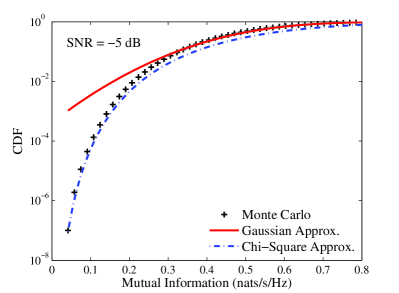
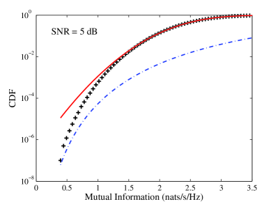
Figure 6: CDF of mutual information for small SNRs, comparing the Gaussian approximation, chi-square approximation, and Monte Carlo simulations. Results are shown for $n_{t}=4$, $n_{r}=2$.

This requires computing the higher order correction terms (in $P$), a task which appears difficult via direct expansion of the $\ln\det({\bf I}_{n}+\frac{P}{m}{\bf HH^{\dagger}})$ formula, as indicated above for the leading order chi-square approximation. To our knowledge, such refinement has not been computed thus far.

To develop a systematic method for solving this refinement problem, we may once again make use of our Painlevé representation. Noting that $x$ is large whilst the new variable $y$ is finite, we assume the following large-$x$ expansion:

$$Y(y)=Y_{0}(y)+\frac{Y_{1}(y)}{x}+\frac{Y_{2}(y)}{x^{2}}+\cdots\;.$$ (111)

Substituting (111) into (21) and matching the coefficient of $x^{-k}$, we can compute $Y_{k}(y)$ systematically in closed-form. For example,

$$Y_{1}(y)=-\frac{\beta(\beta+1)y}{(y-1)^{3}}\;.$$ (112)

Integrating $Y_{1}(y)$ through (VI-B), we obtain the CGF with first-order correction term (in $P$):

$$\mathcal{K}(\lambda)\approx-mn\ln\left(1-\frac{P}{m}\lambda\right)-\frac{n}{2}\frac{(1+1/\beta)\lambda P^{2}}{\left(\lambda P/m-1\right)^{2}}\;.$$ (113)

With this, the saddle point (83) is obtained as

$$t=\frac{mnP\left[-2\lambda^{\star 2}P^{2}+(nP^{2}+mP^{2}+4mP)\lambda^{\star}-2m^{2}+mnP+m^{2}P\right]}{2\left(\lambda^{\star}P-m\right)^{3}}\;.$$ (114)

This expression can be solved in closed-form, with the resulting expression involving a cubic equation. Alternatively, one may trivially compute the solution numerically for any given value of $t$. With $\lambda^{\star}$ solved for a given $t$, the value of the rate function $I(t)$ and thus $\widetilde{I}(t)$ follow immediately according to the definitions (84) and (96) respectively (with $\mu$ and $\sigma^{2}$ in (96) approximated via $\mu_{0}$ and $\sigma_{0}^{2}$). By invoking the CDF formula (102), we can then compute the saddle point approximation for the mutual information distribution. This approximation is illustrated in Fig. 7. Compared with the chi-square approximation, it is shown that this refined CDF is remarkably accurate, even for moderate $P$ values (e.g., $P=10\,{\rm dB}$). As $P$ further increases (beyond, for example, $P=15{\rm dB}$), we have found that the saddle point approximation starts to miss the correct behavior, and higher order correction terms (equivalently, $Y_{2}(y),Y_{3}(y),\ldots$) are needed. These can be systematically computed using the same procedure as before.

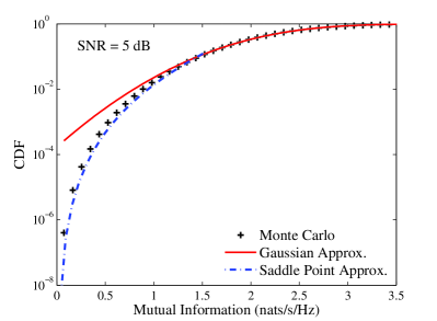
(a) $n_{t}=2,\;n_{r}=2$

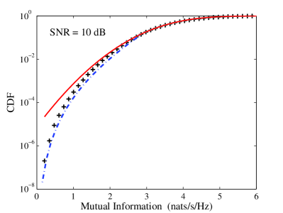
(b) $n_{t}=2,\;n_{r}=2$

Figure 7: CDF of mutual information for small SNRs, comparing the Gaussian approximation, saddle point approximation, and Monte Carlo simulations. Results are shown for $n_{t}=2$, $n_{r}=2$ and for different SNRs.

VI-C Asymptotic CGF at Large SNR

Now we consider the large-$n$–large-$P$ scenario. Based on the expressions which have been computed for $C_{\ell,0},\ell=1,2,\ldots$ for $P\to\infty$ (e.g., (58)–(60)), we obtain the generic expression for the leading term of the $\ell$-th cumulant ($\ell\geq 3$):

$$\kappa_{\ell}\sim\left(-1\right)^{\ell}\left(\ell-3\right)!\left[\frac{1}{\left(m-n\right)^{\ell-2}}-\frac{1}{m^{\ell-2}}\right]\;,\quad\ell=1,2,\ldots\;.$$ (115)

With this, upon summing the CGF series, the asymptotic CGF is computed in closed form:

$$\mathcal{K}(\lambda) \approx\mu_{0}\lambda+\frac{\sigma_{0}^{2}}{2}\lambda^{2}+\sum_{\ell=3}^{\infty}\frac{\left(\ell-3\right)!}{\ell!}\left(-\lambda\right)^{\ell}\left[\frac{1}{\left(m-n\right)^{\ell-2}}-\frac{1}{m^{\ell-2}}\right]$$ (116)

$$=\left(\mu_{0}\!-\!\frac{n}{2}\right)\lambda\!+\!\frac{\sigma^{2}_{0}}{2}\lambda^{2}\!+\!\frac{(\lambda\!+\!m)^{2}}{2}\ln\left(1\!+\!\frac{\lambda}{m}\right)\!-\!\frac{(\lambda\!+\!m\!-\!n)^{2}}{2}\ln\left(1\!+\!\frac{\lambda}{m\!-\!n}\right).$$ (117)

Now, from (1) and (2), we have

$$\mu_{0}\approx n\ln{P}-(m-n)\ln\left(\frac{m-n}{m}\right)-n\;,\qquad P\to\infty,$$ (118)

$$\sigma_{0}^{2}\approx\ln\left(\frac{m}{m-n}\right)\;,\qquad P\to\infty,$$ (119)

giving the following large-$n$–large-$P$ CGF:

$${\cal K}\left(\lambda\right) \approx\left[n\ln\left(\frac{P}{m}\right)-\frac{3}{2}n\right]\lambda+\frac{\left(m+\lambda\right)^{2}}{2}\ln\left(m+{\lambda}\right)$$

$$-\frac{\left(m-n+\lambda\right)^{2}}{2}\ln\left(m-n+{\lambda}\right)-\frac{m^{2}}{2}\ln{m}+\frac{(m-n)^{2}}{2}\ln{(m-n)}\;,$$ (120)

valid for $\lambda\in(n-m,+\infty)$.

Remark 3

Interestingly, although (VI-C) was obtained based on the cumulant expressions which are valid only for $\beta\neq 1$ (i.e., since a singularity exists for $\beta=1$ in the $n$-asymptotic cumulants, as seen in (58)–(60)), by setting $\beta=1$, we have

$${\cal K}\left(\lambda\right) \approx n\lambda\ln\left(\frac{P}{n}\right)-\frac{3}{2}n\lambda+\frac{\left(n+\lambda\right)^{2}}{2}\ln\left(n+{\lambda}\right)$$

$$-\frac{\lambda^{2}}{2}\ln{\lambda}-\frac{n^{2}}{2}\ln{n}\;.$$ (121)

This will be shown to describe the correct behavior of the mutual information.

The saddle point (83) can be computed by

$$t=n\ln P-n\ln m-n+(m+\lambda^{\star})\ln(m+\lambda^{\star})-(m-n+\lambda^{\star})\ln(m-n+\lambda^{\star}).$$ (122)

Whilst a closed-form solution for (122) is intractable, it can be trivially computed numerically for any given value of $t$.

By invoking (85) and (102), we can compute the distribution (both the PDF and CDF) of the mutual information. We should point out that $t$ in (122) is a monotonically increasing function of $\lambda$ (i.e., ${\rm d}t(\lambda)/{\rm d}\lambda>0$), thus for any $t\geq n\ln\left(P/\beta\right)-n$, there exists a real root $\lambda^{\star}$. This, in turn, implies that the distribution cannot be captured explicitly by (122) if $t$ is sufficiently small such that $\mu-t>m\ln\left({\beta}\right)-(m-n)\ln(\beta-1)$ (i.e., when looking sufficiently far into the left tail region). Nevertheless, the right-hand side of this inequality is increasing with $m$ (fixed $n$); thus as $m$ grows, the valid region of (122) extends further into the left tail, allowing smaller outage probabilities to be calculated. In fact, scenarios for which $m$ is reasonably large compared with $n$ is quite realistic in many applications; for example, in cellular systems, for which the base station may be equipped with a reasonably large number of antennas, whilst the number of antennas on the mobile device is more restricted due to limited space constraints.

Fig. 8 depicts the saddle point approximation of the PDF (85) with $I(t)$ computed from (VI-C) and (122), comparing with the Gaussian approximation and Monte Carlo simulations. The saddle point result is clearly much more accurate than the Gaussian, and lines up almost perfectly with the simulations when the SNR is sufficiently large (i.e., at $30$ dB). Similar observations are made in Fig. 9, which shows the corresponding CDF curves based on (102) and the same $I(t)$. Note that for these results we have chosen $m=6,\;n=2$, where $m$ is comparatively large enough such that the validity of (122) extends deep enough into the left tail region to capture outage probabilities of interest.

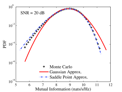
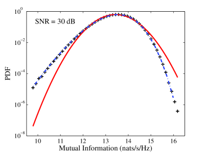
Figure 8: PDF of mutual information, comparing the Gaussian approximation, saddle point approximation, and Monte Carlo simulations. Results are shown for $n_{t}=6,\;n_{r}=2$ and for different SNRs.

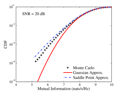
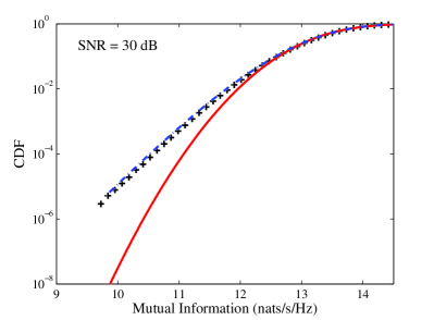
Figure 9: CDF of mutual information, comparing the Gaussian approximation, saddle point approximation, and Monte Carlo simulations. Results are shown for $n_{t}=6,\;n_{r}=2$ and for different SNRs.

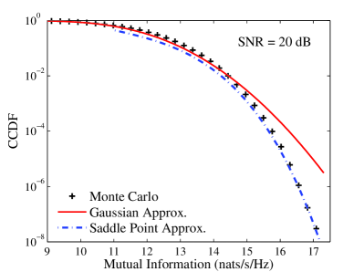
(a) $n_{t}=n_{r}=3$

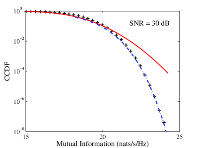
(b) $n_{t}=n_{r}=3$

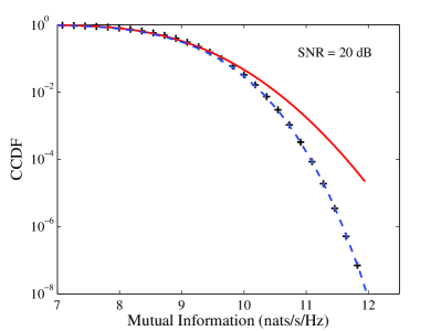
(c) $n_{t}=4,\;n_{r}=2$

Figure 10: CCDF of mutual information, comparing the Gaussian approximation, saddle point approximation, and Monte Carlo simulations. Results are shown for different antenna configurations and different SNRs.

Fig. 10 depicts the complementary CDF (CCDF) of the mutual information, comparing the saddle point approximation based on $I(t)$ computed from (VI-C) and (122), the Gaussian approximation, and Monte Carlo simulations. As for the left tail, we see that the saddle point approximation becomes extremely accurate when the SNR is sufficiently high, and significantly outperforms the Gaussian approximation. In fact, quite surprisingly, even for moderate SNRs of $20$ dB, the saddle point approximation in the right-hand tail traces the simulated curve very closely.

As done for the small-SNR scenario, for large-SNR we can also evaluate the higher order correction terms (in $P$) in order to draw insight into the accuracy of the leading-order results. To this end, it is convenient to first introduce the change of variables $x\to\beta/x$ in the Painlevé representation of the CGF (9) and the large-$n$ equation (21). The CGF to leading order in $n$ can then be written as

$$\mathcal{K}(n\lambda)\sim-n^{2}\int_{0}^{P}\frac{Y(\beta/x)}{x}{\rm d}x,\qquad n\to\infty,$$ (123)

with $Y(\beta/x)$ satisfying

$$\left[xY^{\prime}+\left(1+\frac{\lambda+1}{\beta}\right)x^{2}Y^{\prime}+Y\right]^{2}=4\left(-xY^{\prime}-Y+\beta\right)\left(\frac{x^{2}}{\beta}Y^{\prime}-\lambda\right)\left(\frac{x^{2}}{\beta}Y^{\prime}\right)$$ (124)

where $Y^{\prime}:={\rm d}Y(\beta/x)/{\rm d}x$. By noting that in (VI-C) there exists first-order terms in $P$ which are $O(\ln P)$ and second-order terms which are $O(1)$, we assume that the CGF admits the following generic large-$P$ expansion:

$$\mathcal{K}(n\lambda)=n^{2}\left(\lambda\ln P+b_{0}+\frac{b_{1}}{P}+\frac{b_{2}}{P^{2}}+\cdots\right)$$ (125)

where the coefficient $b_{0}$ denotes the constant term in (VI-C) and $b_{i},i=1,2,\ldots$ depend on $\beta$ and $\lambda$. Taking the derivative of $\mathcal{K}(n\lambda)$ w.r.t. $P$, we obtain the following power series expansion:

$$Y\left(\frac{\beta}{P}\right) =-P\frac{\rm d}{{\rm d}P}\left(\frac{\mathcal{K}(n\lambda)}{n^{2}}\right),\qquad n\to\infty$$

$$=-\lambda+\frac{b_{1}}{P}+\frac{2b_{2}}{P^{2}}+\cdots$$ (126)

Substituting (VI-C) into (124) and matching coefficients of the powers series of $P$ on the left and right-hand sides, we solve the $b_{i}$’s:

$$b_{1}=\frac{\lambda\beta}{\beta+\lambda-1}\;,$$

$$b_{2}=-\frac{\beta^{2}\lambda\left(\beta-1\right)\left(\beta+\lambda\right)}{2\left(\beta+\lambda-1\right)^{4}}\;,$$

$$b_{3}=\frac{\beta^{3}\lambda(\beta-1)(\beta+\lambda)(\beta+\lambda+1)(\beta-1-\lambda)}{3\left(\beta+\lambda-1\right)^{7}}\;,$$

$$\;\,\vdots$$ (127)

Together with (125), we obtain the large-$n$–large-$P$ CGF with higher correction terms in $P$:

$$\mathcal{K}(\lambda)\sim\mathcal{K}_{0}(\lambda)+\frac{mn\lambda}{m-n+\lambda}\frac{1}{P}-\frac{m^{2}(m-n)(m+\lambda)}{2n(m-n+\lambda)^{4}}\frac{1}{P^{2}}+\cdots\quad n\to\infty,\quad P\to\infty$$ (128)

where $\mathcal{K}_{0}(\lambda)$ denotes the leading-order large-$n$–large-$P$ CGF expression in (VI-C). Based on this formula, we draw the following remarks:

• First, we see that the higher correction terms vanish rapidly as $m-n+\lambda$ increases (equivalently, $\lambda$ grows for fixed $m$ and $n$). Meanwhile, as $\lambda$ decreases and approaches $n-m$, the correction terms become large and eventually invalidate the expansion. This indicates that the leading-order large-$n$–large-$P$ approximation for the right-hand tail (corresponding to positive $\lambda$) is more robust for finite values of $P$, compared with the approximation for the left-hand tail (corresponding to negative $\lambda$). This is consistent with the results shown in Figs. 9 and 10.

• Interestingly, as we keep computing $b_{i}$’s, it is found that $b_{i},i>1$ have the common factor of $m-n$. Assuming this is true for all higher correction terms, then for equal antenna arrays (i.e., $m=n$), we have

  $$\mathcal{K}(\lambda)\sim\mathcal{K}_{0}(\lambda)+\frac{n^{2}}{P}\;,\qquad n\to\infty\;.$$ (129)

  Note that the single correction term $n^{2}/P$ is independent of $\lambda$, meaning that the saddle point equation (122) (after setting $m=n$) is unaffected by including correction terms for finite $P$. This agrees with the formula in [27, Eq. (53)] and the corresponding argument made therein.

Based on (128), we plot the saddle point approximation with first-order correction term (in $P$) in Fig. 11. The refinement brought by including the correction term is clearly evident. Moreover, we find that the right-hand tail is captured accurately for moderate $P=15\;{\rm dB}$ even without the first-order correction, which is in line with the discussion in the first point above.

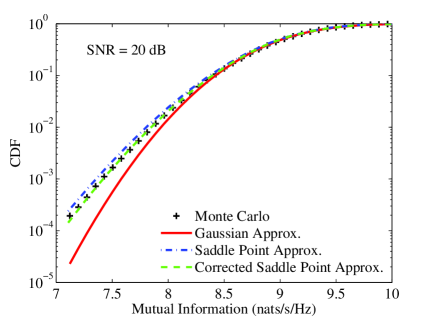
(a) $n_{t}=10,n_{r}=2$

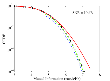
(b) $n_{t}=4,n_{r}=2$

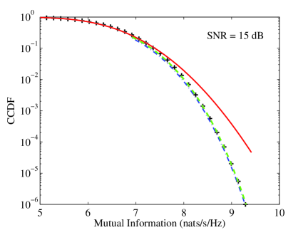
(c) $n_{t}=4,n_{r}=2$

Figure 11: CDF and CCDF of mutual information, comparing the Gaussian approximation, the saddle point approximation with and without the first order corrections (in $P$), and Monte Carlo simulations. Results are shown for different antenna configurations and different SNRs.

VI-D Important Large SNR Behavior in Left and Right Tails (Including DMT)

In this section, we develop further our analytical results under the assumption that $t=qn\ln P,\;P\to\infty$, where $q>0$ is a fixed constant. This represents the setting where the data rate is specified to grow as a non-vanishing fraction (i.e., $q$) of the mean mutual information for large $P$ (i.e., $n\ln P$). This assumption is important in various contexts; for example, in specifying the fundamental DMT [29], as well as capturing the scheduling gains in opportunistic multi-user downlink transmissions [22].

We begin with the scenario $q\geq 1$, in which case we are interested in the mutual information distribution at the right-hand side of the mean. This scenario is relevant for evaluating the performance of scheduling algorithms for which the multi-antenna base-station transmits to the multi-antenna user with the best channel (i.e., $\mathcal{I}_{\rm best}=\max\{\mathcal{I}_{1},\mathcal{I}_{2},\ldots\}$, with $\mathcal{I}_{k}$ denoting the mutual information between the base-station and the $k$th user, all of which are assumed to be independent and to undertake the same distribution). In this case, the mutual information achieved by the system will typically be above the mean mutual information for each user $\mu$, and the performance gains of such “best user” selection algorithms can be characterized by studying the distribution of the per-user mutual information in the regime $t\geq\mu$. See [22] and [27].

Substituting $t=qn\ln P,q\geq 1$ into (122), we have the following asymptotic solution:

$$\lambda^{\star}\sim nP^{q-1}\;,\quad P\to\infty$$ (130)

which further yields

$$I(t) \sim n^{2}P^{q-1}\ln P^{q}$$

$$=\frac{nt}{P}e^{t/n}\;,\qquad P\to\infty.$$ (131)

Therefore, for high $P$, the CCDF admits

$${\Pr(\mathcal{I}({\bf x;y})>t})\sim e^{-\frac{nt}{P}e^{t/n}},\quad t\geq\mu\;.$$ (132)

This agrees with a result derived recently in [27, Eq. (79)], by asymptotically solving a set of coupled equations obtained via a Coulomb fluid formulation. From (132), we find the probability of the mutual information taking greater values than the mean drops very sharply (doubly exponentially with $t$), indicating that for large SNR, the best-user scheduling algorithm indicated above will not enhance the overall data rate significantly.

Now we consider the alternative regime, $q<1$, corresponding to the DMT framework seminally proposed by [29]. In this case, however, we find that one cannot simply adopt the direct approach of substituting $t=qn\ln P$ with $q<1$ into (122), since a solution for the asymptotic $\lambda^{\star}$ does not exist. This can be explained by noting that the solution in fact lies in the range $\lambda^{\star}<n-m$ which can not be described by (VI-C), because $t=qn\ln P<n\ln(P/\beta)-n$ (i.e., the smallest value of $t$ that can be covered by (122)) for $q<1$ and large $P$. Nevertheless, in the following, we are able to draw upon the exact characterization of the large-$n$–large-$P$ CGF (21) to derive the DMT formula.

Since in the large deviation regime, $\lambda^{\star}\sim O(n)$ such that all the cumulants to leading order in $n$ remain effective for large $n$, we scale the CGF variable $\lambda\to n\lambda$ before taking $n\to\infty$ in (133). Further, by recalling the definition of the CGF, its leading order representation in $P$ should be $O(\ln P)$. Consequently, the asymptotic characterization of the CGF admits

$$\mathcal{K}(n\lambda)\approx-n^{2}\;\int_{0}^{P}\frac{Y(\beta/x)}{x}{\rm d}x\approx\;A\;n^{2}\ln P,\qquad n\to\infty,\quad P\to\infty$$ (133)

where $Y(\beta/x)$ satisfies (124) and $A$ denotes a certain function of $\beta$ and $\lambda$. In light of the DMT formulation [29], we require the coefficient of the $O(n^{2}\ln P)$ term of the CGF, i.e., the quantity

$$A=\lim_{P\to\infty}\left(-\frac{1}{\ln P}\int_{0}^{P}\frac{Y(\beta/x)}{x}{\rm d}x\right)\;.$$ (134)

Note here that we cannot employ the assumption $Y(\beta/x)=\sum_{k=0}^{\infty}b_{k}/x^{k}$, since integrating this power series diverges for each term. This motivates us to introduce suitable variable transformations to (123) and (124) as described below, which are aimed at scaling $x$ to increase with $P$, whilst keeping the new variable of integration finite. To this end, observe that

$$-\frac{1}{\ln P}\int_{0}^{P}\frac{Y(\beta/x)}{x}{\rm d}x =-\frac{1}{\ln P}\int_{\epsilon}^{P}\frac{Y(\beta/x)}{x}{\rm d}x-\frac{1}{\ln P}\int_{0}^{\epsilon}\frac{Y(\beta/x)}{x}{\rm d}x$$ (135)

$$=-\int_{\ln\epsilon/\ln P}^{1}Y(\beta/x){\rm d}\left(\frac{\ln x}{\ln P}\right)-\frac{1}{\ln P}\int_{0}^{\epsilon}\frac{Y(\beta/x)}{x}{\rm d}x$$ (136)

$$\sim-\int_{0}^{1}Y(\beta/P^{s})\;{\rm d}s\;,\quad P\to\infty$$ (137)

where the new variable $s:=\ln x/\ln P$ and $\epsilon$ is an arbitrarily small constant. Here $\epsilon$ is introduced to avoid the singularity at the lower limit when changing ${\rm d}x/x$ on the right-hand side of (135) to ${\rm d}(\ln x)$ in (136). Nevertheless, for fixed $\epsilon$, the second integral in (136) vanishes as $P\to\infty$ and the lower limit of the first integral becomes zero, thus we arrive to the asymptotic formula (137). With (137) we have

$$A=\lim_{P\to\infty}\left(-\int_{0}^{1}Y(\beta/P^{s})\;{\rm d}s\right)$$ (138)

with $Y(\beta/P^{s})$ satisfying

$$\left[\frac{Y^{\prime}}{\ln P}+\left(\frac{\beta+\lambda+1}{\beta}\right)\frac{P^{s}}{\ln P}Y^{\prime}+Y\right]^{2}=4\left(-\frac{Y^{\prime}}{\ln P}-Y+\beta\right)\left(\frac{P^{s}}{\beta\ln P}Y^{\prime}-\lambda\right)\frac{P^{s}}{\beta\ln P}Y^{\prime}$$ (139)

where $Y^{\prime}:={\rm d}Y(\beta/P^{s})/{\rm d}s$. By comparing the coefficient of $P^{s}/\ln P$ (i.e., the terms corresponding to the leading order in $P$) in (139), we have the equation involving $Y(\beta/P^{s})$:

$$\left(\frac{P^{s}}{\beta\ln P}Y^{\prime}\right)^{2}\left[4Y-4\beta+\left(\beta+\lambda+1\right)^{2}\right]=0,$$ (140)

which gives a constant solution

$$Y(\beta/P^{s})=-\frac{(\beta+\lambda+1)^{2}}{4}+\beta\;.$$ (141)

Thus we obtain the large-$n$–large-$P$ CGF via (137) and (133):

$$\mathcal{K}(n\lambda)\sim n^{2}\left[\frac{(\beta+\lambda+1)^{2}}{4}-\beta\right]\ln P\;,\qquad n\to\infty,\quad P\to\infty\;.$$ (142)

By invoking the saddle point equation (83): $qn\ln P=\frac{\rm d}{{\rm d}(n\lambda)}\mathcal{K}(n\lambda)$, we have $\lambda^{\star}=2q-\beta-1$. This result reconfirms our statement that the DMT cannot be described by (122), which implicitly requires $n\lambda^{\star}>n-m$. With this saddle point, the rate function $I(t)$ (with $t=qn\ln P,\;q<1$) is evaluated as

$$I(qn\ln P)=qn^{2}\lambda^{\star}\ln P-\mathcal{K}(n\lambda^{\star})=n^{2}\left[q^{2}-q(\beta+1)+\beta\right]\ln P\;.$$ (143)

Consequently, the CDF of the mutual information in the left tail for large $P$ (and large $n$) becomes

$$\ln{\rm Pr}(\mathcal{I}({\bf x;y})<qn\ln P)\sim-\left(qn-m\right)\left(qn-n\right)\ln P,\quad x<\mu\;.$$ (144)

This agrees precisely with the well known DMT result in [29].

VII Conclusion

Capitalizing upon the exact Painlevé based representation for the MGF of the MIMO mutual information in [24], we have systematically computed new expansions for the high order cumulants of the mutual information distribution which apply for arbitrary SNRs and for asymmetric antenna arrays. In particular, closed-form expressions were given for the leading order terms (in $n$), as well as the first-order correction terms which capture finite-antenna deviations. Based on these new expressions, we established key novel insights into the behavior of the distribution under different conditions; for example, explaining why the $n$-asymptotic Gaussian approximation is more robust to increasing SNRs for asymmetric systems compared with symmetric systems. This is an interesting phenomenon which appears difficult to capture with other methods. In addition, we called upon the Edgeworth expansion technique along with the high order cumulant formulas to provide closed-form refinements to the Gaussian approximation for the tail region corresponding to $O(n^{\epsilon})$ ($0<\epsilon\leq 1$) deviations from the mean. For deviations of $O(n)$, the so-called “large deviations” region, the Edgeworth expansion requires summing over all cumulants and becomes unwieldy; thus, in this region we employed a saddle point approximation technique along with asymptotic integration tools to derive very simple and concise formulas for the CDF for the cases of low and high SNRs. Simulations showed that our results captured the tail distribution very accurately for outage probabilities of practical interest. Moreover, whilst formally derived based on a large-antenna framework, they were shown to be very accurate even when the antenna numbers are small. To emphasize the utility of our framework even further, in the end we recovered well known properties of the tail distribution of the MIMO mutual information, including the DMT.

We conclude by noting that the key analytical tool underpinning the analysis in this paper, the Painlevé based MGF representation in Proposition 1, is extremely valuable since, as we have shown, it facilitates a “unified” investigation of the mutual information distribution under a wider range of scenarios than appear possible with previous existing tools. To the best of our knowledge, together with our recent work [24], this is the first time that such tools have been applied to problems in information theory. It turns out that these tools are also applicable to other problems in information theory and wireless communications, and such topics are currently being pursued.

Appendix: Relation with Coulomb Fluid Method in [27]

Here we draw the connections between our saddle point results and those derived based on a Coulomb fluid large deviation approximation in [27]. We start by recasting the formulation of [27] in terms of the MGF of the mutual information. To this end, consider the exact MGF (II) represented in multi-integral form:

$$\mathcal{M}(\lambda) =\frac{\int_{\mathbb{R}^{n}_{+}}\prod_{k=1}^{n}(1+Py_{k})^{\lambda}y_{k}^{\alpha}e^{-ny_{k}}\prod_{i<j}(y_{i}-y_{j})^{2}{\rm d}\mathbf{y}}{\int_{\mathbb{R}^{n}_{+}}\prod_{k=1}^{n}y_{k}^{\alpha}e^{-ny_{k}}\prod_{i<j}(y_{i}-y_{j})^{2}{\rm d}\mathbf{y}}:=\frac{Z(\lambda)}{Z(0)}$$ (145)

where ${\bf y}=(y_{1},\ldots,y_{n})$ denotes the eigenvalues of ${\bf HH^{\dagger}}$ and

$$Z(\lambda)=\int_{\mathbb{R}^{n}_{+}}\exp\left\{\lambda\sum_{k=1}^{n}(1+Py_{k})+\sum_{k=1}^{n}\left[(m-n)\ln y_{k}-ny_{k}\right]+2\sum_{i<j}\ln\lvert y_{i}-y_{j}\rvert\right\}{\rm d}\mathbf{y}\;.$$ (146)

Based on the Coulomb fluid interpretation (see [45, 46, 47, 48, 49] for details), as $n$ grows large, the CGF associated with (145) is anticipated to be well approximated with the following:

$$\mathcal{K}(\lambda):=\ln\mathcal{M}(\lambda)\approx-\min_{\sigma(y)}F[\sigma(y),\lambda]+\min_{\sigma(y)}F[\sigma(y),0]$$ (147)

where

$$F[\sigma,\lambda]=\int_{a}^{b}\sigma(y) \left\{n^{2}[y-(\beta-1)\ln y]\right\}{\rm d}y-\lambda n\int_{a}^{b}\ln(1+Py)\sigma(y){\rm d}y$$

$$\phantom{n^{2}[y-(\beta-1)}-n^{2}\int_{a}^{b}\int_{a}^{b}\ln\lvert y-z\rvert\sigma(y)\sigma(z){\rm d}y{\rm d}z\;$$ (148)

is the so-called “free energy”, whilst $\sigma(y)$ is a PDF with support $[a,b]$. Meanwhile, we have the saddle point approximation of the density function:

$$p_{\mathcal{I}({\bf x;y})}(t)\sim\exp\{-\max_{\lambda}[t\lambda-\mathcal{K}(\lambda)]\}\;,$$ (149)

which, combined with (147), is equivalent to

$$p_{\mathcal{I}({\bf x;y})}(t)\sim\exp\left\{-\max_{\lambda}\min_{\sigma(y)}\left\{F[\sigma,\lambda]+t\lambda\right\}+\min_{\sigma(y)}F[\sigma,0]\right\}.$$ (150)

Recalling that in the “large deviations” regime of interest, $t\sim O(n),\lambda\sim O(n)$ (see the discussions in Section VI-A), we scale $t\to nt,\lambda\to n\lambda$, and (150) becomes

$$p_{\mathcal{I}({\bf x;y})}(nt)\sim\exp\left\{n^{2}\left\{-\max_{\lambda}\min_{\sigma(y)}f[\sigma,\lambda,t]+\min_{\sigma(y)}f[\sigma,0,0]\right\}\right\}\;,$$ (151)

with

$$f[\sigma,\lambda,t]= \frac{F(n\lambda)}{n^{2}}+t\lambda$$

$$= \int_{a}^{b}\sigma(y)\left([y-(\beta-1)\ln y]\right){\rm d}y+\lambda\left[t-\int_{a}^{b}\ln(1+Py)\sigma(y){\rm d}y\right]$$

$$\qquad\qquad\qquad\qquad-\int_{a}^{b}\int_{a}^{b}\ln\lvert y-z\rvert\sigma(y)\sigma(z){\rm d}y{\rm d}z\;.$$ (152)

We find that (151) coincides exactly with [27, Eq. (23)], where the optimization problems $\max_{\lambda}\min_{\sigma(y)}(\cdot)$ are solved jointly, eventually resulting in three coupled non-linear equations in general.

In contrast, our method first employs the Painlevé equation to obtain the $n$-asymptotic CGF as

$$\mathcal{K}(n\lambda)\sim n^{2}\int_{\infty}^{\beta/P}\frac{G(x)}{x}{\rm d}x,\qquad n\to\infty$$

with $G(x)$ exactly characterized by (10). This representation corresponds to evaluating (147) explicitly, without any intuitive Coulomb fluid analogy. Then, armed with this CGF result, we separately draw upon the saddle point equation to capture the tail distribution, which corresponds to solving (149). Thus, in essence, our saddle point approximation is solving the equivalent problem to that considered in [27] by explicitly finding the asymptotic CGF (whilst in [27] it is implicit). Quite remarkably, under the high and low SNR regimes considered, it also leads to simplified results.

References

- [1] H. Bölcskei, R. U. Nabar, Ö. Oyman, and A. J. Paulraj, “Capacity scaling laws in MIMO relay networks,” IEEE Trans. Wireless Commun., vol. 5, no. 6, pp. 1433–1444, Jun. 2006.
- [2] Y. Fan and J. Thompson, “MIMO configurations for relay channels: Theory and practice,” IEEE Trans. Wireless Commun., vol. 6, no. 5, pp. 1774–1786, May 2007.
- [3] J. Wagner, B. Rankov, and A. Wittneben, “Large analysis of amplify-and-forward MIMO relay channels with correlated Rayleigh fading,” IEEE Trans. Inf. Theory, vol. 54, no. 12, pp. 5735–5746, Dec. 2008.
- [4] P. Dharmawansa, M. R. McKay, and R. K. Mallik, “Analytical performance of amplify-and-forward MIMO relaying with orthogonal space-time block codes,” IEEE Trans. Inf. Theory, vol. 58, no. 7, pp. 2147–2158, Jul. 2010.
- [5] S. Jin, M. R. McKay, C. Zhong, and K.-K. Wong, “Ergodic capacity analysis of amplify-and-forward MIMO dual-hop systems,” IEEE Trans. Inf. Theory, vol. 56, no. 5, pp. 2204–2224, May 2010.
- [6] M. Yuksel and E. Erkip, “Multiple-antenna cooperative wireless systems: A diversity-multiplexing tradeoff perspective,” IEEE Trans. Inf. Theory, vol. 53, no. 10, pp. 3371–3393, Oct. 2007.
- [7] D. Gesbert, S. Hanly, H. Huang, S. Shamai (Shitz), O. Simeone, and W. Yu, “Multi-cell MIMO cooperative networks: A new look at interference,” vol. 28, no. 9, pp. 1380–1408, Dec. 2010.
- [8] H. Dahrouj and W. Yu, “Coordinated beamforming for the multicell multi-antenna wireless system,” IEEE Trans. Wireless Commun., vol. 9, no. 5, pp. 1748–1759, May 2010.
- [9] T. Liu and S. Shamai (Shitz), “A note on the secrecy capacity of the multiple-antenna wiretap channel,” IEEE Trans. Inf. Theory, vol. 55, no. 6, pp. 2547–2553, Jun. 2009.
- [10] A. Mukherjee and A. L. Swindlehurst, “Robust beamforming for security in MIMO wiretap channels with imperfect CSI,” IEEE Trans. Signal Process., vol. 59, no. 1, pp. 351–361, Jan. 2011.
- [11] F. Oggier and B. Hassibi, “The secrecy capacity of the MIMO wiretap channel,” IEEE Trans. Inf. Theory, vol. 57, no. 8, pp. 4961–4972, Aug. 2011.
- [12] B. Chen and M. J. Gans, “MIMO communications in ad hoc networks,” IEEE Trans. Signal Process., vol. 54, no. 7, pp. 2773–2783, Jul. 2006.
- [13] A. M. Hunter, J. G. Andrews, and S. Weber, “Transmission capacity of ad hoc networks with spatial diversity,” IEEE Trans. Wireless Commun., vol. 7, no. 12, pp. 5058–5071, Dec. 2008.
- [14] R. H. Y. Louie, M. R. Mckay, and I. B. Collings, “Open-loop spatial multiplexing and diversity communications in ad hoc networks,” IEEE Trans. Inf. Theory, vol. 57, no. 1, pp. 317–344, Jan. 2011.
- [15] Y. Wu, R. H. Y. Louie, M. R. McKay, and I. B. Collings, “Generalized framework for the analysis of linear MIMO transmission schemes in decentralized wireless ad hoc networks,” IEEE Trans. Wireless Commun., 2012, to appear. [Online]. Available: http://ieeexplore.ieee.org/stamp/stamp.jsp?tp=&arnumber=6205593.
- [16] Z. Wang and G. B. Giannakis, “Outage mutual information of space-time MIMO channels,” IEEE Trans. Inf. Theory, vol. 50, pp. 657–662, Apr. 2004.
- [17] H. Shin, M. Z. Win, and J. H. Lee, “Saddlepoint approximation to the outage capacity of MIMO channels,” IEEE Trans. Wireless Commun., vol. 5, no. 10, pp. 2697–2684, Oct. 2006.
- [18] Ö. Oyman, R. U. Nabar, H. Bölcskei, and A. J. Paulraj, “Characterizing the statistical properties of mutual information in MIMO channels,” IEEE Trans. Signal Process., vol. 51, no. 11, pp. 2784–2795, Nov. 2003.
- [19] P. J. Smith, L. M. Garth, and S. Loyka, “Exact capacity distribution for MIMO systems with small numbers of antennas,” IEEE Commun. Lett., vol. 7, no. 10, pp. 481–483, Oct. 2003.
- [20] P. J. Smith and L. M. Garth, “Exact capacity distribution for dual MIMO systems in Ricean fading,” IEEE Commun. Lett., vol. 8, no. 1, pp. 18–20, Jan. 2004.
- [21] A. L. Moustakas, S. H. Simon, and A. M. Sengupta, “MIMO capacity through correlated channels in the presence of correlated interferers and noise: A (not so) large analysis,” IEEE Trans. Inf. Theory, vol. 49, no. 10, pp. 2545–2561, Oct. 2003.
- [22] B. M. Hochwald, T. L. Marzetta, and V. Tarokh, “Multi-antenna channel hardening and its implications for rate feedback and scheduling,” IEEE Trans. Inf. Theory, vol. 50, no. 9, pp. 1893–1909, Sep. 2004.
- [23] W. Hachem, O. Khorunzhiy, P. Loubaton, J. Najim, and L. Pastur, “A new approach for capacity analysis of large dimensional multiantenna channels,” IEEE Trans. Inf. Theory, vol. 54, pp. 3987–4004, Sep. 2008.
- [24] Y. Chen and M. R. McKay, “Coulomb fluid, Painlevé transcendents and the information theory of MIMO systems,” IEEE Trans. Inf. Theory, vol. 58, no. 7, pp. 4594–4634, Jul. 2012.
- [25] P. B. Rapajic and D. Popescu, “Information capacity of a random signature multiple-input multiple-output channel,” IEEE Trans. Commun., vol. 48, no. 8, pp. 1245–1248, Aug. 2000.
- [26] A. L. Moustakas, S. H. Simon, and A. M. Sengupta, “Statistical mechanics of multi-antenna communications: Replicas and correlations,” Acta Physica Polonica Series B, vol. 36, no. 9, pp. 2719–2732, Sep. 2005.
- [27] P. Kazakopoulos, P. Mertikopoulos, A. L. Moustakas, and G. Caire, “Living at the edge: A large deviations approach to the outage MIMO capacity,” IEEE Trans. Inf. Theory, vol. 57, no. 4, pp. 1984–2007, Apr. 2011.
- [28] S. Li, Y. Chen, and M. R. McKay, “Mutual information distribution of interference-limited MIMO: A joint Coulomb fluid and Painlevé based approach,” in Proc. of the th Asilomar Conference on Signals, Systems and Computers, Pacific Grove, CA, USA, Nov. 6-Nov. 9, 2011, pp. 774–778.
- [29] L. Zheng and D. N. C. Tse, “Diversity and multiplexing: A fundamental tradeoff in multiple-antenna channels,” IEEE Trans. Inf. Theory, vol. 49, no. 5, pp. 1073–1096, May 2003.
- [30] İ. E. Telatar, “Capacity of multi-antenna Gaussian channels,” Europ. Trans. Telecommun., vol. 10, no. 6, pp. 585–595, Nov-Dec. 1999.
- [31] E. Biglieri, J. Proakis, and S. Shamai, “Fading channels: Information-theoretic and communications aspects,” IEEE Trans. Inf. Theory, vol. 44, no. 6, pp. 2619–2692, Oct. 1998.
- [32] A. Magnus, “Painlevé-type differential equations for the recurrence coefficients of semi-classical orthogonal polynomials,” J. Comput. Appl. Math., vol. 57, no. 1-2, pp. 215–237, 1995.
- [33] Y. Chen and A. R. Its, “Painlevé III and a singular linear statistics in Hermitian random matrix ensembles,” J. Approx. Theory, vol. 162, no. 2, pp. 270–297, 2010.
- [34] E. Basor and Y. Chen, “Perturbed Hankel determinants,” J. Phys. A: Math. Gen., vol. 38, no. 47, pp. 10 101–10 106, 2005.
- [35] T. L. Marzetta, “Noncooperative cellular wireless with unlimited numbers of base station antennas,” IEEE Trans. Wireless Commun., vol. 9, no. 11, pp. 3590–3600, Nov. 2010.
- [36] H. Q. Ngo, E. G. Larsson, and T. L. Marzetta, “Analysis of the pilot contamination effect in very large multicell multiuser MIMO systems for physical channel models,” in Proc. of IEEE International Conference on Acoustics Speech and Signal Processing, Prague, Czech Repulic, May 2011, pp. 3464–3467.
- [37] ——, “Energy and spectral efficiency of very large multiuser MIMO systems,” IEEE Trans. Commun., submitted. [Online]. Available: http://arxiv.org/abs/1112.3810.
- [38] F. Rusek, D. Persson, B. K. Lau, E. G. Larsson, T. L. Marzetta, O. Edfors, and F. Tufvesson, “Scaling up MIMO: Opportunities and challenges with very large arrays,” IEEE Signal Processing Mag., 2012, to appear. [Online]. Available: http://liu.diva-portal.org/smash/get/diva2:450781/FULLTEXT01.
- [39] B. Gopalakrishnan and N. Jindal, “An analysis of pilot contamination on multi-user MIMO cellular systems with many antennas,” in Proc. of IEEE 12th International Workshop in Signal Processing Advances in Wireless communications, San Francisco, CA, USA, Jun. 2011, pp. 381–385.
- [40] A. Lozano, A. M. Tulino, and S. Verdú, “High-SNR power offset in multi-antenna communication,” IEEE Trans. Inf. Theory, vol. 51, no. 12, pp. 4134–4151, Dec. 2005.
- [41] A. Grant, “Rayleigh fading multiple-antenna channels,” EURASIP J. Applied Signal Processing, Special Issue on Space-Time Coding (Part I), vol. 2002, no. 3, pp. 316–329, Mar. 2002.
- [42] S. Blinnikov and R. Moessner, “Expansions for nearly Gaussian distributions,” Astron. Astrophys. Suppl. Ser., no. 130, pp. 193–205, May 1998.
- [43] H. E. Daniels, “Saddlepoint approximations in statistics,” Ann. Math. Statistics, vol. 25, no. 4, pp. 631–650, 1954.
- [44] I. Avramidi, “Lecture notes on asymptotic expansion,” Oct. 2000, [Online]. Available: http://www.nmt.edu/~iavramid/notes/asexp.pdf.
- [45] F. J. Dyson, “Statistical theory of energy levels of complex systems I-III,” J. Math. Phys., vol. 3, no. 1, pp. 140–175, 1962.
- [46] Y. Chen and S. M. Manning, “Asymptotic level spacing of the Laguerre ensemble: A Coulomb fluid approach,” J. Phys. A.:Math. Gen., vol. 27, no. 11, pp. 3615–3620, 1994.
- [47] Y. Chen and N. D. Lawrence, “On the linear statistics of Hermitian random matrices,” J. Phys. A: Math. Gen., vol. 31, no. 4, pp. 1141–1152, 1998.
- [48] Y. Chen and S. M. Manning, “Distribution of linear statistics in random matrix models (metallic conductance fluctuations),” J. Phys.: Condens. Matter, vol. 6, no. 16, pp. 3039–3044, 1994.
- [49] Y. Chen and M. E. H. Ismail, “Thermodynamic relations of the Hermitian matrix ensembles,” J. Phys. A: Math. Gen., vol. 30, no. 19, pp. 6633–6654, 1997.