The cosmological information of shear peaks: beyond the abundance

Abstract

We study the cosmological information of weak lensing (WL) peaks, focusing on two other statistics besides their abundance: the stacked tangential-shear profiles and the peak-peak correlation function. We use a large ensemble of simulated WL maps with survey specifications relevant to future missions like $\it{Euclid}$ and lsst, to measure and examine the three peak probes. We find that the auto-correlation function of peaks with high signal-to-noise (${\mathcal{S}}/{\mathcal{N}}$) ratio measured from fields of size 144 $\rm deg^{2}$ has a maximum of $\sim 0.3$ at an angular scale $\vartheta\sim 10$ arcmin. For peaks with smaller ${\mathcal{S}}/{\mathcal{N}}$, the amplitude of the correlation function decreases, and its maximum occurs on smaller angular scales. The stacked tangential-shear profiles of the peaks also increase with their ${\mathcal{S}}/{\mathcal{N}}$. We compare the peak observables measured with and without shape noise and find that for ${\mathcal{S}}/{\mathcal{N}}\sim 3$ only $\sim 5\%$ of the peaks are due to large-scale structures, the rest being generated by shape noise. The correlation function of these small peaks is therefore very weak compared to that of small peaks measured from noise-free maps, and also their mean tangential-shear profile is a factor of a few smaller than the noise-free one. The covariance matrix of the probes is examined: the correlation function is only weakly covariant on scales $\vartheta<30$ arcmin, and slightly more on larger scales; the shear profiles are very correlated for $\vartheta>2$ arcmin, with a correlation coefficient as high as 0.7. The cross-covariance of the three probes is relatively weak: the peak abundance and profiles have the largest correlation coefficient $\sim 0.3$. Using the Fisher-matrix formalism, we compute the cosmological constraints for $\{{\Omega_{\rm m}},\,{\sigma_{8}},\,w,\,{n_{\rm s}}\}$ considering each probe separately, as well as in combination. We find that the peak-peak correlation and shear profiles yield marginalized errors which are larger by a factor of $2-4$ for $\{{\Omega_{\rm m}},\,{\sigma_{8}}\}$ than the errors yielded by the peak abundance alone, while the errors for $\{w,\,{n_{\rm s}}\}$ are similar. By combining the three probes, the marginalized constraints are tightened by a factor of $\sim 2$ compared to the peak abundance alone, the least contributor to the error reduction being the correlation function. This work therefore recommends that future WL surveys use shear peaks beyond their abundance in order to constrain the cosmological model.

1 Introduction

With the approach of large weak gravitational lensing (WL) missions, such as $\it{Euclid}$ and lsst (LSST Science Collaborations et al., 2009; Laureijs et al., 2011), it is imperative to optimize the extraction of cosmological information from WL probes. Until now, the WL community has been using mainly the 2-point function of the shear field in order to obtain cosmological constraints (Jarvis et al., 2003; Hoekstra et al., 2006; Semboloni et al., 2006; Hetterscheidt et al., 2007; Kilbinger et al., 2012), and also to plan and forecast coming missions (Laureijs et al., 2011). Whilst a lot of effort is concentrated on scrutinizing the systematics of WL surveys – a most essential endeavour for the success of the next-generation missions, and indeed for the future of WL as a cosmology probe – the task of selecting the most efficient statistics for parameter estimation is also a crucial aspect that should not be neglected.

One of the possible WL observables involves the ‘peaks’ of the shear field, i.e. regions of high signal-to-noise (${\mathcal{S}}/{\mathcal{N}}$) of the field, produced by overdense regions of the density field projected along the line of sight. Shear peaks are the imprint of clusters in WL maps, and can be used to detect and measure cluster masses (Hamana et al., 2004; Wang et al., 2004; Maturi et al., 2005; Hennawi & Spergel, 2005; Dahle, 2006; Marian & Bernstein, 2006; Schirmer et al., 2007; Maturi et al., 2007; Abate et al., 2009). The peak abundance scales with cosmological parameters in the same way as the halo mass function (Reblinsky et al., 1999; Marian et al., 2009, 2010), and therefore can be used to constrain the cosmological model (Dietrich & Hartlap, 2010; Kratochvil et al., 2010; Marian et al., 2012; Bard et al., 2013). The shear-peak abundance can also constrain primordial non-Gaussianity (Marian et al., 2011; Maturi et al., 2011; Hilbert et al., 2012), and so far seems to be possibly the most effective WL observable suitable for that purpose – although more work must be done on this subject.

Whilst the abundance of peaks has been investigated by a number of studies, higher-order statistics of the shear peaks have until now been overlooked. Yet, since the abundance of peaks can be used as a cosmological tool, one would expect their clustering to also be valuable. In analogy with 3D observables, just as both the halo correlation function and the halo mass function are very sensitive to cosmology, the same could be true about the shear peaks.

The main goal of this study is to investigate the correlation function of WL peaks, and in particular to quantify the improvements that it yields on cosmological constraints relative to the peak abundance. As a secondary line of inquiry, we shall also pursue the cosmological information contained in the tangential-shear profiles of the peaks. While these statistics – correlations and stacked profiles of overdensities – have been already studied in various theoretical works, as well as by using real and simulated data (Sheldon et al., 2004; Sheldon et al., 2009; Mandelbaum et al., 2010; Oguri & Takada, 2011; Mandelbaum et al., 2012; Cacciato et al., 2012), here we explore the characteristics of shear-selected overdensities for which the only known information is the redshift distribution of the source galaxies. This might seem a somewhat unlikely and conservative scenario for future surveys, but here we just examine the intrinsic information contained in the peaks, even if our results will be sub-optimal on this account. We defer to a near-future study a more realistic scenario, where prior information on the peaks is available, and where we can account for various survey uncertainties, such as intrinsic alignments, masked regions, calibration errors of the source galaxies, etc.

We shall present measurements of the peak function, peak-peak correlation function, and peak profiles from an ensemble of WL maps generated with ray-tracing through $N$-body simulations with varying cosmologies, as described in §2. We shall use the Fisher-matrix formalism to establish the cosmological sensitivity of the above-mentioned probes. We underscore that our results are drawn from collaborative efforts, which involved generating the $N$-body simulations, the ray-tracing maps, developing the hierarchical algorithm for WL peaks; the present study is part of a larger research program, which has also yielded the results published in Marian et al. (2011, 2012) and Hilbert et al. (2012). Therefore, we shall not give a full description of all our tools, but simply refer to these publications.

The paper is partitioned as follows: in §2, we provide a description of the ray-tracing maps used in this study; in §3 we illustrate our measurements of the three peak probes; in §4 we present the cosmological constraints extracted from the three probes; in §5 we summarize and conclude.

2 Simulated WL maps

We generated WL maps from ray-tracing through $N$-body simulations. We used 8 simulations which are part of a larger suite performed on the zBOX-2 and zBOX-3 supercomputers at the University of Zürich. For all realizations 11 snapshots were output between redshifts $z=[0,2]$; further snapshots are at redshifts $z=\{3,4,5\}$. We shall refer to these simulations as the zHORIZON simulations, and they were described in detail in Smith (2009); Smith et al. (2012). Each of the zHORIZON simulations was performed using the publicly available Gadget-2 code (Springel, 2005), and followed the nonlinear evolution under gravity of $N=750^{3}$ equal-mass particles in a comoving cube of length $L_{\rm sim}=1500\,h^{-1}{\rm Mpc}$; the softening length was $l_{\rm soft}=60\,\,h^{-1}{\rm kpc}$. The cosmological model was similar to that determined by the WMAP experiment (Komatsu et al., 2009). We refer to this cosmology as the fiducial model. The transfer function for the simulations was generated using the publicly available cmbfast code (Seljak & Zaldarriaga, 1996), with high sampling of the spatial frequencies on large scales. Initial conditions were set at redshift $z=50$ using the serial version of the publicly available 2LPT code (Scoccimarro, 1998; Crocce et al., 2006). Table 1 summarizes the cosmological parameters that we simulated. We also use another series of simulations, identical in every way to the fiducial model, except that we have varied one of the cosmological parameters by a small amount. For each new set we have generated 4 simulations, matching the random realization of the initial Gaussian field with the corresponding one from the fiducial model. The four parameter variations were: $\{n\rightarrow(0.95,1.05),\,{\sigma_{8}}\rightarrow(0.7,0.9),\,{\Omega_{\rm m}}\rightarrow(0.2,0.3),\,w\rightarrow(-1.2,-0.8)\}$, and we refer to each of the sets as zHORIZON-V1a,b,…,zHORIZON-V4a,b, respectively.

For the WL simulations, we considered a survey similar to $\it{Euclid}$ (Laureijs et al., 2011) and to lsst (LSST Science Collaborations et al., 2009), with: an rms $\sigma_{\gamma}=0.3$ for the intrinsic image ellipticity, a source number density $\bar{n}=40\,\mathrm{arcmin}^{-2}$, and a redshift distribution of source galaxies given by ${\mathcal{P}}(z)={\cal N}(z_{0},\beta)\,z^{2}\exp[-(z/z_{0})^{\beta}],$

Table 1: zHORIZON cosmological parameters. Columns are: density parameters for matter, dark energy and baryons; the equation of state parameter for the dark energy; normalization and primordial spectral index of the power spectrum; dimensionless Hubble parameter.

Cosmological parameters	${\Omega_{\rm m}}$	$\Omega_{\rm DE}$	$\Omega_{b}$	$w$	${\sigma_{8}}$	$n$	$H_{0}[{\rm km}s^{-1}{\rm Mpc}^{-1}]$
zHORIZON-I	0.25	0.75	0.04	-1	0.8	1.0	70.0
zHORIZON-V1a/V1b	0.25	0.75	0.04	-1	0.8	0.95/1.05	70.0
zHORIZON-V2a/V2b	0.25	0.75	0.04	-1	0.7/0.9	1.0	70.0
zHORIZON-V3a/V3b	0.2/0.3	0.8/0.7	0.04	-1	0.8	1.0	70.0
zHORIZON-V4a/V4b	0.25	0.75	0.04	-1.2/-0.8	0.8	1.0	70.0

where the normalization constant ${\cal N}$ ensures that the integral of the source distribution over the source redshift is unity. If this interval extended to infinity, then the normalization could be written analytically as: ${\cal N}=3/(z_{0}^{3}\,\Gamma[(3+\beta)/\beta])$. There is a small difference between this value and what we actually used, due to the fact that we considered a source interval of $[0,3]$. We took $\beta=1.5$, and required that the median redshift of this distribution be $z_{\mathrm{med}}=0.9$, which fixed $z_{0}\approx 0.64$, and gave a mean of $z_{\rm mean}=0.95$.

From each $N$-body simulation we generated 16 independent fields of view. Each field had an area of $12\times 12\,\rm deg^{2}$ and was tiled by $4096^{2}$ pixels, yielding an angular resolution $\theta_{\mathrm{pix}}=10\,\mathrm{arcsec}$. For each variational model, the total area was of $\approx 9000\,\rm deg^{2}$, while for the fiducial model it was of $\approx 18000\,\rm deg^{2}$. The effective convergence $\kappa$ in each pixel was calculated by tracing a light ray back through the simulation with a multiple-lens-plane ray-tracing algorithm (Hilbert et al., 2007, 2009). Gaussian shape noise with variance $\sigma_{\gamma}^{2}/(\bar{n}\,\theta_{\mathrm{pix}}^{2})$ was then added to each pixel, creating a realistic noise level and correlation in the filtered convergence field (Hilbert et al., 2007). We keep the shape noise configuration fixed for each field in different cosmologies, in order to minimize its impact on the comparisons of the peak abundances measured for each cosmology.

3 WL peaks as a cosmological probe

As stated in §1, we shall consider the cosmological information contained in three shear peak probes: the abundance, the profiles, and the correlation function. Until now, only the abundance of peaks has been examined as a probe for cosmology; in this study we shall investigate the cosmological information contained in the clustering of peaks and their profiles, as well as various combinations of the three probes.

The peaks are detected with an aperture-mass filter, i.e. a compensated filter Schneider (1996), as points of maxima in the smoothed convergence field. They are assigned a unique ${\mathcal{S}}/{\mathcal{N}}$ and mass using the hierarchical algorithm. This method, as well as the NFW-shaped filter function, were described in detail in our previous work Marian et al. (2012). The hierarchical algorithm uses a hierarchy of filters of different size, from the largest down to the smallest, to determine the size of the NFW filter that best matches each peak. For every filter used, we write the aperture mass and the ${\mathcal{S}}/{\mathcal{N}}$ at a given point ${\mbox{\boldmath$\theta$}}_{0}$ as

$${M_{\rm ap}}({\mbox{\boldmath$\theta$}}_{0})={M_{\rm m}}\frac{\int d^{2}\theta\,[{\kappa_{\rm m}}(\theta)-{\bar{\kappa}_{\rm m}}(\theta_{\rm A})]\kappa({\mbox{\boldmath$\theta$}}_{0}-{\mbox{\boldmath$\theta$}})}{\int d^{2}\theta\,{\kappa^{2}_{\rm m}}(\theta)-\pi\theta^{2}_{A}{\bar{\kappa}^{2}_{\rm m}}(\theta_{A})},$$ (1)

$${\mathcal{S}}/{\mathcal{N}}({\mbox{\boldmath$\theta$}}_{0})=\sqrt{\frac{\bar{n}}{\sigma_{\gamma}^{2}}}\,\frac{\int d^{2}\theta\,[{\kappa_{\rm m}}(\theta)-{\bar{\kappa}_{\rm m}}(\theta_{\rm A})]\kappa({\mbox{\boldmath$\theta$}}_{0}-{\mbox{\boldmath$\theta$}})}{\sqrt{\int d^{2}\theta\,[{\kappa_{\rm m}}(\theta)-{\bar{\kappa}_{\rm m}}(\theta_{\rm A})]^{2}}},$$ (2)

where ${M_{\rm m}}$ is the mass of the NFW halo used as a model for the filter, and $\theta_{\rm A}$ is the aperture radius of the filter, which in our case was chosen to be the angular size of its NFW radius. ${\kappa_{\rm m}}$ is the convergence profile of the model, ${\bar{\kappa}_{\rm m}}$ is the mean convergence inside a certain radius, and $\kappa$ is the measured convergence field. If ${\mbox{\boldmath$\theta$}}_{0}$ is the location of a peak generated by an NFW halo matching the filter, then the above equations become

$${M_{\rm ap}}({\mbox{\boldmath$\theta$}}_{0})={M_{\rm m}},$$ (3)

$${\mathcal{S}}/{\mathcal{N}}({\mbox{\boldmath$\theta$}}_{0})=\sqrt{\frac{\bar{n}}{\sigma_{\gamma}^{2}}\,\int d^{2}\theta\,[{\kappa_{\rm m}}(\theta)-{\bar{\kappa}_{\rm m}}(\theta_{\rm A})]^{2}}.$$ (4)

The hierarchical method enhances the detection of peaks, their abundance as a function of mass or ${\mathcal{S}}/{\mathcal{N}}$ is independent of any particular choice of filter size, and the cosmological constraints arising from the peak counts are tighter compared to the case when a single-sized filter is used. It is also instructive to present measurements of the peak function, the profiles and the peak-peak correlation function from noise-free maps. In that case, the peaks are selected based on their aperture-mass values, and they are assigned a hierarchical mass through Eq. (3), as described in Marian et al. (2012). For the purpose of comparison with the results from the noisy maps, we can assign the noise-free peaks a fictitious ${\mathcal{S}}/{\mathcal{N}}$ value, using Eqs (3) and (4) with the same level of shape noise as in the noisy maps.

3.1 The peak-peak correlation function

Figure 1: The correlation function of the peaks detected in the maps corresponding to the fiducial cosmological model. The results show the average of 128 fields of $12\times 12\,\rm deg^{2}$ and the error bars represent errors on the mean. Left panel: The orange squares/green triangles denote measurements in the absence of shape noise, for peaks with ${\mathcal{S}}/{\mathcal{N}}\geq 3.4$, and $3.4>{\mathcal{S}}/{\mathcal{N}}\geq 2.6$ respectively. Right panel: Measurements from the noisy maps: the solid red circles, blue squares, green triangles represent the auto-correlation of peaks with ${\mathcal{S}}/{\mathcal{N}}\geq 4.75$, $4.75>{\mathcal{S}}/{\mathcal{N}}\geq 3.4$, $3.4>{\mathcal{S}}/{\mathcal{N}}\geq 2.6$ respectively. In both panels, the purple crosses depict the cross-correlation of the peak populations with $3.4>{\mathcal{S}}/{\mathcal{N}}\geq 2.6$ and ${\mathcal{S}}/{\mathcal{N}}\geq 4.75$, where we have used Eqs (3) and (4) to assign an ${\mathcal{S}}/{\mathcal{N}}$ value to the peaks.

Figure 2: Tangential-shear profiles for the peaks detected in the maps corresponding to the fiducial cosmological model. Left panel: The effect of shape noise on the profiles. The red solid pentagons represent peaks detected in the noise-free maps, with ${\mathcal{S}}/{\mathcal{N}}\geq 4.75$. The green empty squares depict the profiles of these very same peaks, detected in the noisy maps. Similarly, the orange solid squares show the profiles of all the peaks that we detected in the noise-free maps, while the purple stars show the profiles of the same peaks when detected and measured in the noisy maps. Right panel: The profiles measured from the noisy maps: the solid red circles, blue squares, and green triangles represent peaks with ${\mathcal{S}}/{\mathcal{N}}$ indicated in the legend. The purple circles depict all the measured peaks binned together.

We have measured the correlation function of the peaks using the minimum-variance and unbiased estimator introduced by Landy & Szalay (1993). The estimator is:

$$\hat{\omega}_{\rm pp}=(DD-2DR+RR)/RR,$$ (5)

where $DD$, $DR$, and $RR$ represent the peak-peak, peak-random peak, and random peak-random peak pair counts, respectively. The correlation function is measured in 10 angular bins, logarithmically spaced between $\vartheta\in\left[4,90\right]$ arcmin. The lower bound was chosen to be the smallest possible without discreteness effects contaminating the measurements – the latter appear when the size of the lower bins is only a small multiple of the size of the pixels of the map. The random catalogue that we created in order to build the correlation function estimator contained a million random peaks placed in a field of $12\times 12\,\rm deg^{2}$, i.e. the same size as the simulated maps.

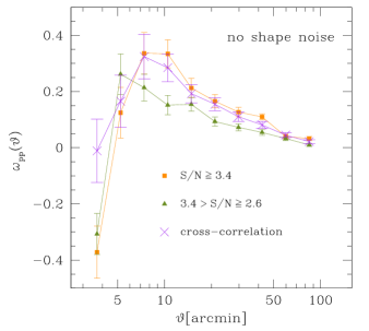
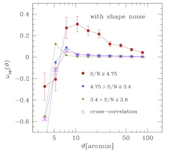
In Figure 1 we present measurements of the correlation function of peaks detected from the maps corresponding to the fiducial cosmology. All symbols denote the average of 128 realizations, the errors being on the mean. The estimator of the average correlation function is defined by Eq. (12); a similar estimator will also be used to obtain the average tangential-shear profile of the peaks and the average peak function presented later in this section.

The left panel of Figure 1 shows the noise-free results, while in the right one shape noise is included. The solid orange squares/green triangles in the left panel depict the auto-correlation $\omega_{\rm pp}^{\rm a}$ of the peaks with $3.4\geq{\mathcal{S}}/{\mathcal{N}}\geq 2.6$ and ${\mathcal{S}}/{\mathcal{N}}\geq 3.4$, respectively. The solid red circles, blue squares, and green triangles in the right panel correspond to peaks with ${\mathcal{S}}/{\mathcal{N}}\geq 4.75$, $4.75\geq{\mathcal{S}}/{\mathcal{N}}\geq 3.4$, and $3.4\geq{\mathcal{S}}/{\mathcal{N}}\geq 2.6$ respectively. The total number of peaks in these bins is $\sim 10,000,\,72,000,\,324,000$ respectively. In both panels, the violet crosses depict the cross-correlation $\omega_{\rm pp}^{\rm c}$ of the bins $3.4\geq{\mathcal{S}}/{\mathcal{N}}\geq 2.6$ and ${\mathcal{S}}/{\mathcal{N}}\geq 4.75$.

The correlation functions are strongly negative for the smallest bins due to an exclusion effect arising from our peak selection: we discard those peaks whose centres are separated from the centre of a larger peak by a distance smaller than approximately one virial radius. The reason for this choice is to avoid classifying substructures as independent peaks.

In general, the peaks with higher/lower ${\mathcal{S}}/{\mathcal{N}}$ have higher/lower correlations, similar to the clustering properties displayed by 3D halos. For the noiseless measurements, the maximum of the auto-correlation of peaks with ${\mathcal{S}}/{\mathcal{N}}\geq 3.4$ is reached at $\sim 8\,\mathrm{arcmin}$ and is about 0.35, while for the peaks with $3.4\geq{\mathcal{S}}/{\mathcal{N}}\geq 2.6$ the maximum is about 0.25 and it is shifted towards smaller scales $\sim 5\,\mathrm{arcmin}$. The auto-correlation functions decrease monotonically to $0$ with increasing angular scales. The same pattern is followed by the correlation functions of the peaks measured from the noisy maps: the higher the ${\mathcal{S}}/{\mathcal{N}}$ bin, the larger the amplitude of the function and the angular position of its maximum. For the largest peaks, a maximum of $\sim 0.3$ is reached at $\sim 10$ arcmin. Comparing the measurements from noise-free and noisy maps allows us to understand how shape noise impacts the correlation function of the peaks. For example, the green triangles in the left and right panels of Figure 1 are dissimilar, although peaks from the same ${\mathcal{S}}/{\mathcal{N}}$ bin are used for the measurements. The noise-free correlation function is significantly higher, dropping to 0 only at $\sim 100\,\mathrm{arcmin}$, unlike its noisy counterpart, which vanishes at $\sim 8\,\mathrm{arcmin}$. The vanishing owes to the fact that most peaks in this ${\mathcal{S}}/{\mathcal{N}}$ bin are generated by shape noise – see also Figure 3 – and behave essentially like random points. The genuine signal seen in the left panel of the figure is ‘drowned’ by the large number of shape-noise pair counts. The same is true for the cross-correlation signal depicted by the purple crosses in both panels. The noise-free signal is quite high, similar to the auto-correlation of peaks with ${\mathcal{S}}/{\mathcal{N}}\geq 3.4$, and the error bars are significantly smaller than for the auto-correlation of the peaks with ${\mathcal{S}}/{\mathcal{N}}\geq 4.75$ – high-${\mathcal{S}}/{\mathcal{N}}$ peaks are very scarce in the noise-free maps, hence the errors on their correlation function are quite large, which is the reason why we do not even show it in the figure. Regarding the noisy maps, whilst the cross-correlation function has a smaller signal-to-noise than the auto-correlation of the largest peaks, it can be used to constrain cosmology, as shown in §4.

3.2 The tangential-shear profiles of the peaks

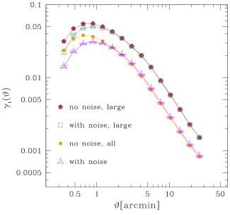
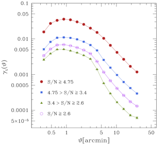
We measure the tangential-shear profiles $\gamma_{T}$ around the centres of the peaks, as found through our filtering method. We use 15 angular bins, logarithmically spanning the interval $\vartheta\in[0.3,26]\,\mathrm{arcmin}$. In Figure 2 we present the average of the stacked profiles, measured from 128 fields corresponding to the fiducial cosmology.

The left panel shows the impact of shape noise on the peak profiles. The solid red pentagons and orange squares depict the stacked profiles of the largest peaks (${\mathcal{S}}/{\mathcal{N}}\geq 4.75$), and all the peaks identified in the noise-free maps. The number of peaks contributing to the two curves are $\sim 4,500$ and $\sim 39,000$ respectively. The noise-free peaks are generated by lensing of large-scale structures (LSS); therefore, they are also present in the noisy maps, albeit with slightly different centre coordinates and amplitude. We match the coordinates of the noise-free peaks to the coordinates of the peaks in the noisy maps. This is done on a field-by-field basis, allowing for a displacement of 5 pixels around the centre of the noise-free peaks. The green empty squares and purple stars indicate the stacked profiles of the same peaks depicted by the solid red pentagons and orange squares, when measured from the noisy maps. The shape noise renders the measured profiles shallower on small scales, $\vartheta\leq\,2\,\mathrm{arcmin}$, due to the shift in the centre coordinates. On scales $\vartheta>\,2\,\mathrm{arcmin}$ there is no significant difference between the noise-free and noisy profiles.

Figure 3: The peak function measured from the maps corresponding to the fiducial cosmological model. The results show the average of 128 fields of 144 $\rm deg^{2}$. The red points denote measurements in the absence of shape noise; the blue squares represent measurements from noisy maps, with an ${\mathcal{S}}/{\mathcal{N}}$-threshold of 2.6.

The right panel shows measurements from the noisy maps. The ${\mathcal{S}}/{\mathcal{N}}$-bins are similar to those used for the correlation function: $3.4>{\mathcal{S}}/{\mathcal{N}}\geq 2.6$ – green solid triangles; $4.75>{\mathcal{S}}/{\mathcal{N}}\geq 3.4$ – blue solid squares; and ${\mathcal{S}}/{\mathcal{N}}\geq 4.75$ – red solid circles. For illustration purposes, we also include the stacked profiles of all peaks binned together, represented by the purple empty circles. The more massive the peaks, the higher their profiles: there is about an order of magnitude difference between the average tangential shear corresponding to the highest and lowest ${\mathcal{S}}/{\mathcal{N}}$-bins. Similar to the correlation function, the stacked profiles of the noisy peaks are significantly lower than the noiseless ones. For example, compare the average profile of all peaks from the two panels, i.e. the orange solid squares on the left with the empty purple circles on the right: there is a factor of $\sim\,5$ difference on small scales, and less on larger scales. This is a consequence of several factors: i) most of the low-${\mathcal{S}}/{\mathcal{N}}$ peaks are caused by shape noise and they represent random points in the shear maps, thereby lowering the profile average of the real peaks; ii) some small genuine LSS peaks are boosted by shape noise above the detection threshold, and so they are included in the right panel, but not in the left one; iii) as shown in the left panel, shape noise does tend to lower the average profiles due to the shifting of the peak centre.

3.3 The peak function

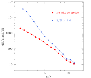
Figure 3 illustrates the peak function $\Phi$, i.e. the number of peaks per unit ${\mathcal{S}}/{\mathcal{N}}$, in a field with area 144 $\rm deg^{2}$. We considered 15 logarithmic ${\mathcal{S}}/{\mathcal{N}}$ bins, in the interval $[2.6,14]$. The red solid circles denote the noiseless peak function measured from 128 fields corresponding to the fiducial cosmology, while the blue solid squares are the same measurement in the presence of shape noise. The two peak functions are very similar at the high-${\mathcal{S}}/{\mathcal{N}}$ end, and differ by a factor of at least 20 at the low-${\mathcal{S}}/{\mathcal{N}}$ end, where peaks generated by shape-noise completely dominate the genuine LSS peaks. Modelling the effect of shape noise on the peak function is the subject of a work in progress, so we shall not dwell on it any longer here. We merely mention that the dominance of shape-noise peaks at the low-${\mathcal{S}}/{\mathcal{N}}$ end of the peak function is in agreement with the behaviour of the peak-peak correlation function, and the tangential-shear profiles displayed in Figures 1 and 2.

4 Fisher matrix calculations

In this section we employ the Fisher-matrix formalism to derive cosmological constraints from the three peak probes presented in the preceding section. We shall make use of the cosmology dependence of our simulated maps, and measure the peak statistics corresponding to the models varying cosmological parameters around the fiducial values. These measurements can then be used to obtain Fisher predictions.

Throughout this work we shall assume the likelihood function of the peak probes to be a multivariate Gaussian. Consider a vector of measurements of the peak-peak correlation function, peak abundance, and peak profiles $\mbox{\boldmath$m$}=\{\omega_{1},\dots,\omega_{n_{\rm B}^{\omega}},\Phi_{1}\dots,\Phi_{n_{\rm B}^{\Phi}},\gamma_{T}^{1},\dots,\gamma_{T}^{\rm n_{\rm B}^{\gamma_{T}}}\}$, where $n_{\rm B}^{\omega},\,n_{\rm B}^{\Phi},\,n_{\rm B}^{\gamma_{T}}$ are the number of bins for the respective measurements. If we similarly define a vector $\bar{\mbox{\boldmath$m$}}$ of the mean of the measurements, we write the likelihood as

$${\cal L}(\mbox{\boldmath$m$}|\,\bar{\mbox{\boldmath$m$}}(\mbox{\boldmath$p$}),\mbox{\boldmath$C$}(\mbox{\boldmath$p$}))=\frac{1}{(2\pi)^{n_{\rm B}/2}|\mbox{\boldmath$C$}|^{1/2}}\hskip 73.97733pt{}$$

$$\times\exp\left[-\frac{1}{2}(\mbox{\boldmath$m$}-\bar{\mbox{\boldmath$m$}})^{t}\mbox{\boldmath$C$}^{-1}(\mbox{\boldmath$m$}-\bar{\mbox{\boldmath$m$}})\right],$$ (6)

where the variable $p$ indicates the dependence on the cosmological model of the mean and covariance matrix of the measurements, in this case specified by: $\{n,\,{\sigma_{8}},\,{\Omega_{\rm m}},\,w\}$. We have also introduced the total number of bins $n_{\rm B}=n_{\rm B}^{\omega}+n_{\rm B}^{\Phi}+n_{\rm B}^{\gamma_{T}}$, as well as the total covariance matrix of the measurements in bins $i$ and $j$:

$$C_{ij}=\langle(m_{i}-\bar{m}_{i})\,(m_{j}-\bar{m}_{j})\rangle,\hskip 14.22636pti,j=\overline{1,n_{\rm B}}$$ (7)

The Fisher matrix is defined as the ensemble-averaged Hessian of the logarithm of the likelihood function,

$${\mathcal{F}}_{\alpha\beta}=-\left<\frac{\partial^{2}\ln{\cal L}}{\partial p_{\alpha}\,\partial p_{\beta}}\right>.$$ (8)

Note that we shall also use Eqs (7) and (8) for each probe individually, case in which the vectors $\mbox{\boldmath$m$},\,\bar{\mbox{\boldmath$m$}}$ and matrix $C$ will implicitly contain only the measurements of the respective probe, and $n_{\rm B}$ will be the number of bins for that same probe. We shall make no further specification on this subject and rely on the context for clarity.

Figure 4: The derivatives of the peak correlation function measured from the noisy maps. The left panel shows the auto-correlation function $\omega_{\rm pp}^{\rm a}$ for peaks with ${\mathcal{S}}/{\mathcal{N}}\geq 4.75$, while in the right one we present the cross-correlation $\omega_{\rm pp}^{\rm c}$ between two bins with low and high ${\mathcal{S}}/{\mathcal{N}}$.

Figure 5: The derivatives of the tangential-shear profiles $\gamma_{T}$ measured from the noisy maps. The left panel corresponds to the peaks detected with ${\mathcal{S}}/{\mathcal{N}}\geq 2.6$, while in the right one, peaks have ${\mathcal{S}}/{\mathcal{N}}\geq 4.75$.

The general expression of Eq. (8) can be rewritten as (Tegmark et al., 1997)

$${\mathcal{F}}_{\alpha\beta}=\frac{1}{2}{\rm Tr}\left[\mbox{\boldmath$C$}^{-1}\mbox{\boldmath$C$}_{,p_{\alpha}}\mbox{\boldmath$C$}^{-1}\mbox{\boldmath$C$}_{,p_{\beta}}\right]+\bar{\mbox{\boldmath$m$}}_{,p_{\alpha}}^{T}{\mbox{\boldmath$C$}}^{-1}\bar{\mbox{\boldmath$m$}}_{,p_{\beta}}.$$ (9)

Here we have denoted by $x_{,p_{\alpha}}=\partial x/\partial p_{\alpha}$. We shall ignore the first term in Eq. (9) for two reasons: i) it is considered to contribute little to the Fisher information – for a discussion on this see Tegmark et al. (1997); ii) an accurate determination of the derivatives of the covariance with respect to the cosmological parameters would require more realizations of the variational cosmologies than we currently have. Therefore we shall follow the standard approach to Fisher-matrix forecasting in the literature and ignore the trace-term in the above equation.

From the Fisher matrix, one may obtain an estimate of the marginalized errors and covariances of the parameters:

$$\sigma^{2}_{p_{\alpha}p_{\beta}}=[{\mathcal{F}}^{-1}]_{\alpha\beta},$$ (10)

as well as the unmarginalized errors:

$$\sigma_{p_{\alpha}}=[{\mathcal{F}}_{\alpha\alpha}]^{-1/2}.$$ (11)

We now turn our attention to the estimation of each element contributing to the simplified expression of the Fisher matrix, discussed above. For each cosmological model, the mean auto- and cross-correlation functions are evaluated as an average of the correlation functions for each field,

$$\hat{\bar{\omega}}(\vartheta)=\frac{1}{n}\sum_{k=1}^{n}\hat{\omega}_{k}(\vartheta),$$ (12)

where $\hat{\omega}_{k}$ is the correlation function measured from the $k^{\rm th}$ field, and $n$ is the number of fields considered. Similarly, we compute the mean of the peak function and the tangential-shear profiles. An unbiased, maximum-likelihood estimator for the covariance is

$$\hat{C}_{ij}=\frac{1}{n-1}\sum_{k=1}^{n}(\hat{m}_{i}^{k}-\hat{\bar{m}}_{i})\,(\hat{m}_{j}^{k}-\hat{\bar{m}}_{j}).$$ (13)

We use this estimator to compute the fiducial-model-covariance matrix for each of the three probes, as well as for any combination of them. The estimate of the inverse covariance is corrected in the following way (Anderson, 1958; Hartlap et al., 2007):

$$\widehat{\mbox{\boldmath$C$}^{-1}}=\frac{n-n_{\rm B}-2}{n-1}(\hat{\mbox{\boldmath$C$}})^{-1},\>n_{\rm B}<n-2,$$ (14)

In order to obtain low-noise estimates of the derivatives with respect to the cosmological parameters, we take advantage of the matched initial conditions of the simulations, and use the double-sided derivative estimator

$$\widehat{\frac{\partial\bar{m}_{i}}{\partial p_{\alpha}}}=\frac{1}{n}\sum_{k=1}^{n}\frac{\hat{m}_{i}^{k}(p_{\alpha}+\Delta\alpha)-\hat{m}_{i}^{k}(p_{\alpha}-\Delta\alpha)}{2\Delta\alpha},$$ (15)

where $\Delta\alpha$ represents the $\pm$ step in the cosmological parameter $p_{\alpha}$, e.g. Table 1. Note that whilst this approach reduces the cosmic variance in the derivatives, the estimated Fisher matrix is still noisy due to the inverse covariance estimator.

Finally, we mention a technical point regarding the joined constraints presented in the next section. Since we evaluate the combined covariance for the three probes, we are concerned that its elements might be very different, hence introducing numerical instabilities in its inversion, and possibly leading to an inaccurate estimate of the inverse. To prevent this, we apply the same strategy recently used in (Smith et al., 2012): instead of using the covariance matrix, we use the correlation matrix, defined by

$$r_{ij}=C_{ij}/\sigma_{i}\,\sigma_{j}\ ,$$ (16)

where $\sigma_{i}=\sqrt{C_{ii}}$ is the rms variance. The inverse correlation and covariance are related by:

$$r^{-1}_{ij}=\sigma_{i}\sigma_{j}C^{-1}_{ij}$$ (17)

We can rewrite the Fisher matrix from Eq. (9) as:

$${\mathcal{F}}_{\alpha\beta}=\sum_{i,j=1}^{n_{\rm B}}\frac{\bar{m}_{i,p_{\alpha}}}{\sigma_{i}}\,{r}_{ij}^{-1}\,\frac{\bar{m}_{j,p_{\beta}}}{\sigma_{j}},$$ (18)

It is this last equation that we shall be using for our forecast, scaling the measured derivatives of the probes by the rms variance of the fiducial functions, and employing the inverse correlation matrix, instead of the inverse covariance.

Figure 6: The derivatives of the peak function $\Phi$ measured from the noisy maps and scaled by the peak function corresponding to the fiducial cosmological model.

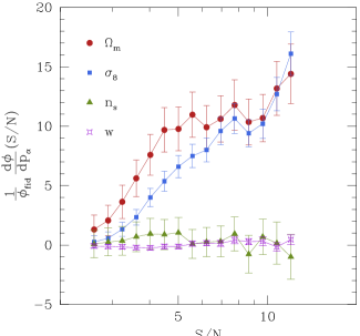
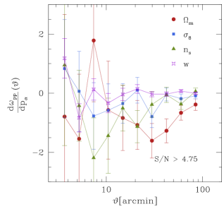
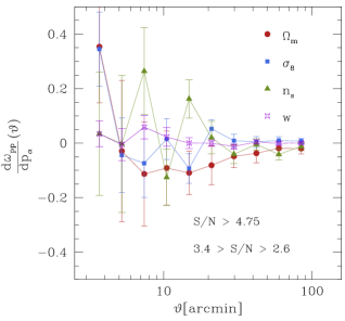
Figure 4 depicts the derivatives of the auto- and cross-correlation function with respect to the cosmological parameters that we investigate in this work – left and right panels, respectively. The auto-correlation derivatives are quite noisy – primarily due to the relatively small number of peaks with ${\mathcal{S}}/{\mathcal{N}}\geq 4.75$, a characteristic also visible in Figure 1, the noise being largest on small scales, $\vartheta<20\,\mathrm{arcmin}$. The ${\Omega_{\rm m}}$- derivative has the largest amplitude, while $w$ has the smallest. All derivatives tend to 0 on larger scales, signifying that there is no information in the peak-peak correlation function for $\vartheta\geq 2\,{\rm deg}$. Compared to the auto-correlation function, the derivatives of the cross-correlation are less noisy, with the exception of ${n_{\rm s}}$. They are also significantly smaller, just like the cross-correlation signal is much smaller than the auto-correlation one. In both panels, the ${\Omega_{\rm m}}$-derivative is negative for $\vartheta\geq 10\,\mathrm{arcmin}$, whilst for the other parameters, the derivatives cross the 0-line a few times.

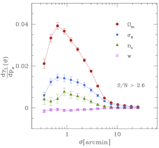
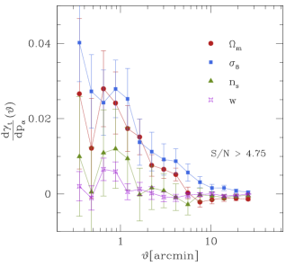
Figure 5 presents the shear-profile derivatives with respect to the cosmological parameters: the left panel corresponds to peaks with ${\mathcal{S}}/{\mathcal{N}}\geq 2.6$, while the right one is for ${\mathcal{S}}/{\mathcal{N}}\geq 4.75$, hence the larger measurement noise present there. In both panels, the derivatives decrease to 0 for increasing angular scales, e.g. $\vartheta\sim 20\,\mathrm{arcmin}$. In the left panel, all derivatives are positive, with the only exception of $w$, which has a barely-noticeable transition from slightly negative to slightly positive. The ${\Omega_{\rm m}}$-derivative is the largest, while the $w$-one is the smallest. For the higher-${\mathcal{S}}/{\mathcal{N}}$ peaks, the derivatives are less smooth, but the general trends are preserved: ${\Omega_{\rm m}}$ and ${\sigma_{8}}$ still have the highest derivatives, followed by ${n_{\rm s}}$ and $w$. They all seem to peak on the scales $0.8-1\,\mathrm{arcmin}$, which suggests that a significant amount of information arises from these scales. We shall mostly be using the larger peaks for our constraints.

Figure 6 depicts the derivatives of the peak function with respect to the cosmological parameters, scaled by the peak abundance corresponding to the fiducial cosmology, as a function of ${\mathcal{S}}/{\mathcal{N}}$. Again ${\Omega_{\rm m}}$ has the largest derivative, followed closely by ${\sigma_{8}}$ – both of them positive. The derivatives with respect to ${n_{\rm s}}$ and $w$ are much smaller and less smooth.

Since in this study we use numerical derivatives to estimate the Fisher errors, as opposed to analytical ones, we need to ask what the resulting uncertainty on the Fisher errors is. This is particularly needed for our noisiest measurements, i.e. for the correlation function. We address this question in the appendix §A, and refer the interested reader to that discussion.

One point of interest – useful mainly to develop one’s intuition – is to explore which are the highest contributing scales to the Fisher information. Naturally, we expect a combination of scales to be the most effective at constraining the cosmological model; the most common approach to determine such a combination is to diagonalize the covariance matrix and determine its eigenvalues: the eigenvectors corresponding to the largest eigenvalues will represent the most constraining linear combinations of scales. To see if there is a particular scale which helps to significantly reduce the errors, we shall take two approaches.

Figure 7: Left panels: Cumulative unmarginalized Fisher errors for $\omega_{\rm pp}^{\rm a}$, $\gamma_{T}$, and $\Phi$ – top, middle, and bottom panels respectively. Bins are added progressively, from small to large scales for the angular bins, and from large to small ${\mathcal{S}}/{\mathcal{N}}$. The cumulative errors are scaled by the final error, i.e. the error obtained when all bins have been included. For the auto-correlation and the profiles, only peaks with ${\mathcal{S}}/{\mathcal{N}}\geq 4.75$ are included. Right panels: The contribution of different scales to the Fisher information, estimated as the rms of Eq. (20).

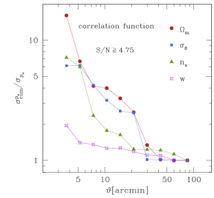
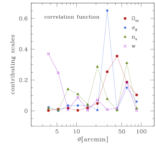
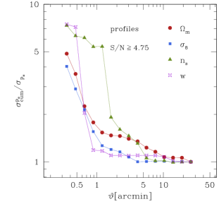
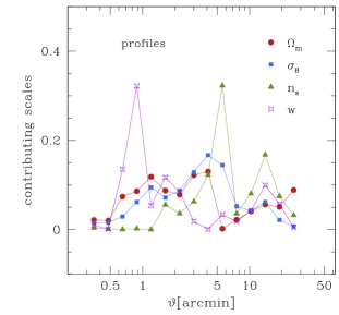
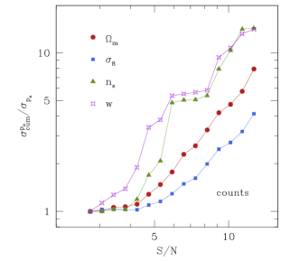
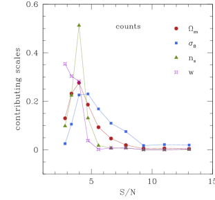
First, we compute the cumulative Fisher matrix, i.e. we monitor how the errors evolve when bins are included one-by-one in the calculation of Eq. (9). We choose as starting bins those containing measurements expected to be easier to perform in real surveys. For example, for the peak counts, we start with the highest-${\mathcal{S}}/{\mathcal{N}}$ bins, and then add progressively smaller-${\mathcal{S}}/{\mathcal{N}}$ bins. For the profiles and correlation functions, we start with small-scale measurements, and progressively include large angular scales. The results of this exercise are presented in the left panels of Figure 7: from top to bottom, we show the cumulative unmarginalized Fisher errors arising from $\omega_{\rm pp}^{\rm a},\,\gamma_{T},$ and $\Phi$, scaled by the final errors – when all bins are included – as a function of bins. For the auto-correlation function, the information seems to saturate at $\sim 40\,\mathrm{arcmin}$: the inclusion of larger-scale measurements does not further improve the constraints. For the profiles, the saturation occurs at $\sim 10\,\mathrm{arcmin}$, while for the peak counts, the inclusion of peaks with ${\mathcal{S}}/{\mathcal{N}}<4$ still improves the constraint on $w$, though not on the other parameters. This is in line with our findings from Marian et al. (2012).

Figure 8: Total cross-correlation matrix of the peak abundance $\Phi$, the peak-peak correlation function $\omega_{\rm pp}^{\rm a}$, and the stacked peak profiles $\gamma_{T}$. $\omega_{\rm pp}^{\rm a}$ and $\gamma_{T}$ are evaluated for peaks with ${\mathcal{S}}/{\mathcal{N}}\geq 4.75$, while $\Phi$ contains the peaks with ${\mathcal{S}}/{\mathcal{N}}\geq 2.6$. From left-right and down-up, we plot the correlations of $\Phi,\,\omega_{\rm pp}^{\rm a},\,\gamma_{T}$, with the ${\mathcal{S}}/{\mathcal{N}}$ and angular scales (measured in $\mathrm{arcmin}$) increasing in the same directions. The correlation matrix is computed from 128 fields of $12\times 12\,\rm deg^{2}$ corresponding to the fiducial cosmology and is rescaled to match a sky coverage of $\sim 18000\,\rm deg^{2}$.

The second approach involves two approximations: i) for each probe we neglect the covariance of the parameters, i.e. we consider only unmarginalized errors – this was also done for the first approach. ii) we disregard the off-diagonal elements of the covariance matrix of each probe. The Fisher matrix can then be written as

$${\mathcal{F}}_{\alpha\alpha}=\sum_{i=1}^{n_{\rm B}}\bar{m}_{i,p_{\alpha}}^{2}/C_{ii}.$$ (19)

We can quantify the contribution of each bin $j$ to the total Fisher constraints through the ratio:

$$\frac{{\mathcal{F}}^{j}_{\alpha\alpha}}{{\mathcal{F}}_{\alpha\alpha}}=\frac{\bar{m}_{j,p_{\alpha}}^{2}/C_{jj}}{\sum_{i=1}^{n_{\rm B}}\bar{m}_{i,p_{\alpha}}^{2}/C_{ii}}.$$ (20)

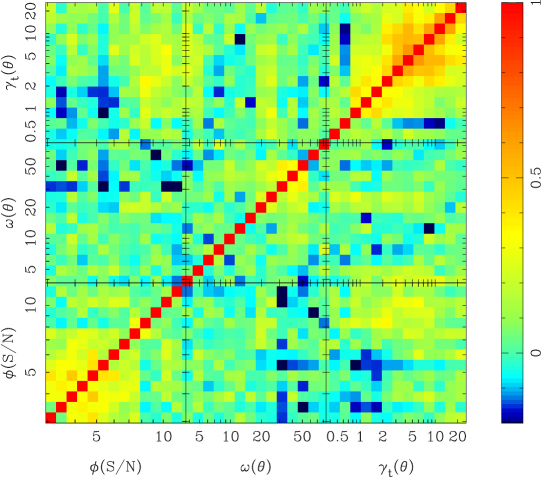
By construction, this ratio works best as a contributing-scales indicator for those probes which have a covariance matrix with as few off-diagonal elements as possible. In our case, this is the auto-correlation function, as can be seen from Figure 8. The rms of the above ratio is shown in the right panels of Figure 7, ordered in the same way as the left ones. For the correlation function, the most contributing scales to the ${\sigma_{8}}$- and ${\Omega_{\rm m}}$-constraints are $\sim 30$ and $\sim 40\,\mathrm{arcmin}$ respectively. This is in agreement with the left panel of the figure: the errors on those two parameters are lowered significantly when the respective bins are included in the Fisher estimates. The constraints from stacked profiles receive contributions from all scales below $10\,\mathrm{arcmin}$, while for the counts the smaller bins (${\mathcal{S}}/{\mathcal{N}}\leq 5$) tighten the errors – though notice that the agreement between the left and right panel is not so good as for the correlation function, due to the high correlations between the low-${\mathcal{S}}/{\mathcal{N}}$ bins. These correlations are included in the left panel, but not in the right one.

5 Cosmological constraints

Figure 9: 2-$\sigma$ Fisher ellipses for the peak probes. The auto-correlation function is depicted by the green dot-dashed ellipse; the red dashed ellipse represents the profiles, while the dotted blue line corresponds to the peak abundance. The combination of the three is given by the black ellipse.

Figure 10: 2-$\sigma$ Fisher ellipses for the peak probes, with a planck-like prior. The colors and symbols are the same as in the previous figure. The prior has been added to each peak probe separately.

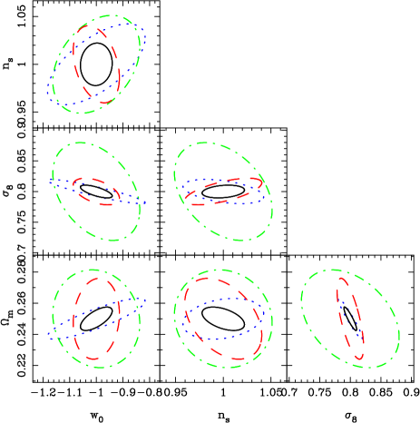
Using all the ingredients described in section §4, we now proceed to constraining the cosmological model using the three peak probes individually, as well as in combination. To this avail, we shall employ only noisy maps, and consider the auto-correlation $\omega_{\rm pp}^{\rm a}$ of peaks with ${\mathcal{S}}/{\mathcal{N}}\geq 4.75$, the cross-correlation $\omega_{\rm pp}^{\rm c}$ of peaks with ${\mathcal{S}}/{\mathcal{N}}\geq 4.75$ and $3.4\geq{\mathcal{S}}/{\mathcal{N}}\geq 2.6$, the stacked profiles $\gamma_{T}$ of peaks with ${\mathcal{S}}/{\mathcal{N}}\geq 4.75$, and the abundance of peaks $\Phi$ with ${\mathcal{S}}/{\mathcal{N}}\geq 2.6$. The Fisher matrix errors are estimated using the covariance on the mean of the fiducial model for the three probes of interest to us here. Thus, our estimated covariance from Eq. (13), which corresponds to an area of $144\,\rm deg^{2}$, is rescaled to correspond to an area 128 times larger, i.e. $\sim 18000\,\rm deg^{2}$. Together with the survey specifications given in section §2, this makes our study representative for two future surveys, lsst and $\it{Euclid}$.

Figure 8 presents the cross-correlation matrix ${\bf r}$ of these probes. By far, $\gamma_{T}$ has the strongest correlation coefficient of the three: $\sim 0.7$ on scales $2-20\,\mathrm{arcmin}$. For the peak function, the low-${\mathcal{S}}/{\mathcal{N}}$ bins are the most correlated $\sim 0.5$ for ${\mathcal{S}}/{\mathcal{N}}\leq 5$. This was already established in our earlier work (Marian et al., 2012), and it can be explained through the better-known behaviour of halos: small-mass halos are sample-variance dominated, while the large and rare halos follow the Poisson distribution (Hu & Kravtsov, 2003; Smith & Marian, 2011). Note however how the smallest-${\mathcal{S}}/{\mathcal{N}}$ bins in Figure 8 seem to be completely uncorrelated: this is most likely due to the overwhelming number of shape-noise peaks, which are random, unclustered, and therefore uncorrelated. $\omega_{\rm pp}^{\rm a}$ displays the smallest correlation coefficient of the three, $\sim 0.3-0.4$ on the scales $20-60\,\mathrm{arcmin}$, with weaker correlations on smaller scales. We further note the weak cross-correlation of $\omega_{\rm pp}^{\rm a}$ and $\Phi$, as well as $\omega_{\rm pp}^{\rm a}$ and $\gamma_{T}$. There is a visible cross-correlation of $\Phi$ and $\gamma_{T}$, of $\sim 0.3$ for peaks with ${\mathcal{S}}/{\mathcal{N}}>7$. This is most likely due to the stacked profiles being dominated by the most massive peaks, which also dominate the high-${\mathcal{S}}/{\mathcal{N}}$ end of the peak function.

Table 2: Fisher-matrix constraints using $\omega_{\rm pp}^{\rm a},\,\omega_{\rm pp}^{\rm c}$, $\gamma_{T}$, and $\Phi$. All errors are presented as percentages of the fiducial values of the parameters, ${{\Omega_{\rm m}}=0.25,\,{\sigma_{8}}=0.8,\,w=-1,\,{n_{\rm s}}=1}$.

Unmarginalized errors [%]

$\omega_{\rm pp}^{\rm a}$ $\omega_{\rm pp}^{\rm c}$ $\gamma_{T}$ $\Phi$ $\omega_{\rm pp}^{\rm a}+\Phi$ $\omega_{\rm pp}^{\rm a}+\gamma_{T}$ $\omega_{\rm pp}^{\rm c}+\Phi$ $\omega_{\rm pp}^{\rm c}+\gamma_{T}$ $\Phi+\gamma_{T}$ $\omega_{\rm pp}^{\rm a}+\Phi+\gamma_{T}$ $\omega_{\rm pp}^{\rm c}+\Phi+\gamma_{T}$ ${\Omega_{\rm m}}$ 3.7 6.7 3.3 0.3 0.3 2.4 0.3 3 0.3 0.3 0.3 ${\sigma_{8}}$ 3.2 3.4 1.8 0.2 0.2 1.4 0.2 1.6 0.2 0.2 0.2 $w$ 5.6 10.2 3.5 1.6 1.5 3 1.5 3.2 1.3 1.3 1.4 ${n_{\rm s}}$ 1.9 1.7 1.6 0.7 0.6 1.1 0.7 1.1 0.6 0.6 0.6

Marginalized errors [%]

$\omega_{\rm pp}^{\rm a}$ $\omega_{\rm pp}^{\rm c}$ $\gamma_{T}$ $\Phi$ $\omega_{\rm pp}^{\rm a}+\Phi$ $\omega_{\rm pp}^{\rm a}+\gamma_{T}$ $\omega_{\rm pp}^{\rm c}+\Phi$ $\omega_{\rm pp}^{\rm c}+\gamma_{T}$ $\Phi+\gamma_{T}$ $\omega_{\rm pp}^{\rm a}+\Phi+\gamma_{T}$ $\omega_{\rm pp}^{\rm c}+\Phi+\gamma_{T}$ ${\Omega_{\rm m}}$ 4.4 6.8 4 1.9 1.4 3 1.5 3.7 1.2 1.1 1.1 ${\sigma_{8}}$ 4.1 4 2 1 0.7 1.8 0.7 1.8 0.6 0.5 0.5 $w$ 6.4 11.5 4 6.7 4.5 3.2 4.5 3.4 2.9 2.7 2.7 ${n_{\rm s}}$ 2.1 2.1 2 1.6 1.2 1.2 1.1 1.3 1 0.8 0.9

Table 2 presents the unmarginalized and marginalized 1-$\sigma$ errors resulting from the three peak probes. Each probe taken by itself, the abundance of peaks has the greatest constraining power, followed by the profiles, and then by the correlation function. Regarding the latter, we note that $\omega_{\rm pp}^{\rm a}$ and $\omega_{\rm pp}^{\rm c}$ yield very similar constraints, the auto-correlation being more effective for $w$ and ${\Omega_{\rm m}}$ – a reduction by factors of $\sim 2$ and $\sim 1.5$ respectively in these errors, compared to the cross-correlation. However, when combined with the other two probes, there is little difference between $\omega_{\rm pp}^{\rm a}$ and $\omega_{\rm pp}^{\rm c}$. The greatest benefit to adding the correlation function or the profiles to the abundance of peaks concerns the time-independent equation-of-state for dark energy: after marginalizing over the other parameters, the errors on $w$ resulting from $\Phi$ and $\omega_{\rm pp}^{\rm a}$ taken individually are similar, while the profiles seem to yield a constraint tighter by a factor of $\sim 1.7$. When all three probes are combined, the constraints on ${\Omega_{\rm m}},\,{\sigma_{8}},\,{n_{\rm s}}$ improve by a factor of $\sim 1.5-2$ compared to using $\Phi$ alone, while for $w$ the improvement is $\sim 2.5$. Lastly, combining $\Phi$ and $\gamma_{T}$ is almost as efficient as using all three probes: the contribution of the correlation functions to reducing the errors is negligible, if both the abundance and the profiles are used.

This is further detailed by Figure 9 which shows the forecasted likelihood contours, at 95% confidence level. The largest ellipses – green, dot-dashed – represent the $\omega_{\rm pp}^{\rm a}$ constraints; for many of the parameter combinations, the red, dashed ellipses depicting $\gamma_{T}$ are almost perpendicularly oriented relative to the $\omega_{\rm pp}^{\rm a}$ ellipses, and also quite tilted with respect to the $\Phi$ ellipses, shown by the blue dotted lines. The greatest gain in combining all three probes is for the case of $w$, where the resulting ellipse is smaller by a factor of $\sim 3$ compared to the $\Phi$ ellipse.

We compare our Fisher constraints to those of Hilbert et al. (2012), derived for an identical survey scenario from the same simulated WL maps. That analysis combines the shear correlation functions, the third moment of the aperture mass, and the peak abundance, and accounts also for local primordial non-Gaussianity. The percentage unmarginalized combined 1-$\sigma$ errors found in Hilbert et al. (2012) for $\{{\Omega_{\rm m}},\,{\sigma_{8}},\,w,\,{n_{\rm s}}\}$ were $\{0.2,\,0.15,\,0.9,\,0.4\}$. The marginalized errors were $\{0.7,\,0.4,\,2.6,\,0.7\}$. Their constraints are tighter, particularly for ${\Omega_{\rm m}}$, but the combination of peak probes performs nonetheless very well.

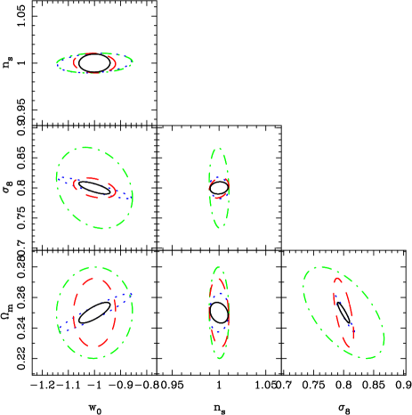
Figure 10 presents the 95%-likelihood contours of the three probes, after we have added cosmic microwave background (CMB) information resulting from an experiment similar to planck. For the latter, we assume that the CMB temperature and polarization spectra can constrain 9 parameters: the dark energy equation-of-state parameters $w_{0}$ and $w_{a}$; the density parameter for dark energy $\Omega_{\rm DE}$; the CDM and baryon density parameters scaled by the square of the dimensionless Hubble parameter $\omega_{\rm CDM}=\Omega_{\rm CDM}\,h^{2}$ and $\omega_{\rm b}=\Omega_{\rm b}\,h^{2}$ ($h=H_{0}/[100\,{\rm km\,s^{-1}\,Mpc^{-1}}]$); the primordial spectral index of scalar perturbations ${n_{\rm s}}$; the primordial amplitude of scalar perturbations $A_{s}$; the running of the spectral index $\alpha$; and the optical depth to the last scattering surface $\tau$. We compute the CMB Fisher matrix as described by Eisenstein et al. (1999):

$${\mathcal{F}}_{\alpha\beta}=\sum_{l}\sum_{X,Y}\frac{\partial C_{l,X}}{\partial p_{\alpha}}{\rm Cov}^{-1}\left[C_{l,X},C_{l,Y}\right]\frac{\partial C_{l,Y}}{\partial p_{\beta}}\ ,$$ (21)

where $\{X,Y\}\in\{{\rm TT},\,{\rm EE},\,{\rm TE},\,{\rm BB}\}$, where $C_{l,\rm TT}$ is the temperature power spectrum, $C_{l,\rm EE}$ is the E-mode polarization power spectrum, $C_{l,\rm TE}$ is the temperature-E-mode polarization cross-power spectrum, and $C_{l,\rm BB}$ is the B-mode polarization power spectrum. The assumed sky coverage is $f_{\rm sky}=0.8$ In order to make the CMB Fisher matrix compatible with our parameters, we rotate it to a new set ${\bf q}^{T}=\{w_{0},w_{a},\Omega_{m},h,f_{b},\tau,{n_{\rm s}},{\sigma_{8}},\alpha\}\ ,$ where for us $w_{0}=w$. We marginalize over the 5 parameters absent from our analysis, and then add the resulting $4\times 4$ matrix to the Fisher matrix for each of the probes, and their combination. This way of implementing the planck prior follows the same steps taken in our previous studies (Marian et al., 2012; Hilbert et al., 2012). Figure 10 shows that combining the peak probes with the CMB dramatically alters all the ellipses involving ${n_{\rm s}}$: they are shrunken and almost completely aligned. This is hardly surprising, as the CMB constrains ${n_{\rm s}}$ much better than any WL probe, so the ellipses are then dominated by the CMB information. For the other parameters, the changes are small, and there is still a significant gain to be obtained by combining the peak probes, compared to using only one of them, for instance the abundance.

6 Summary and conclusion

In this paper we have investigated cosmological constraints from WL peaks, beyond using just counts. We have measured for the first time the peak-peak correlation function, and estimated its constraining power on the following cosmological parameters: $\{{\Omega_{\rm m}},\,{\sigma_{8}},\,w,\,{n_{\rm s}}\}$. We have also measured the tangential-shear profiles of the peaks, and explored their cosmological utility. Whilst both the correlation function and stacked profiles of galaxies/clusters are standard tools for cosmology, our study applies them to shear-selected objects, detected only through their gravitational lensing effects. We employed mostly numerical methods, performing measurements of the peak abundance, peak profiles, and peak-peak correlation functions in simulated WL maps. To estimate the cosmological constraints, we used the Fisher-matrix formalism, computing the derivatives with respect to cosmological parameters and the combined covariance of the three peak probes from the simulated maps. The latter have been generated with ray-tracing through a large suite of $N$-body simulations, varying the cosmological model around some fiducial values. Given the distribution of source galaxies and the level of shape noise considered, our simulated maps are relevant for future large WL missions, such as $\it{Euclid}$ and lsst.

To measure the correlation function of peaks, we used the Landy & Szalay (1993) estimator, known for two essential properties: i) minimum variance; ii) lack of bias due to the unknown mean density of the measured objects. We have shown that the correlation function has its maximum on scales $\vartheta\leq 10\,\mathrm{arcmin}$, with the position and height of the latter depending on the ${\mathcal{S}}/{\mathcal{N}}$ of the considered peaks. For angular scales $\vartheta\geq 8\,\mathrm{arcmin}$, the correlation function of ‘large’ peaks (${\mathcal{S}}/{\mathcal{N}}\geq 4.75$) has a greater amplitude than that of ‘medium’ and ‘small’ peaks ($4.75>{\mathcal{S}}/{\mathcal{N}}\geq 3.4$ and ${\mathcal{S}}/{\mathcal{N}}<3.4$), mirroring the clustering behaviour of dark-matter halos. We have shown that the low-${\mathcal{S}}/{\mathcal{N}}$ end of the peak function is completely dominated by shape-noise peaks – only $\sim 5\%$ of peaks with ${\mathcal{S}}/{\mathcal{N}}\sim 3$ are genuine LSS peaks. This is the reason why the correlation function of the small peaks quickly declines to $0$: shape-noise peaks are random, and therefore uncorrelated. On the contrary, the correlation function of the peaks measured from noise-free maps is quite high, even with all peaks, small and large, binned together: this is just a statement that peaks due genuinely to projected LSS are quite clustered. The cross-correlation of small- and large-${\mathcal{S}}/{\mathcal{N}}$ peaks measured from noisy maps is also smaller than its noise-free counterpart, but it can still be used for cosmological constraints.

We have measured the tangential-shear profiles of the peaks using their WL centre, as detected by our hierarchical method. We found that the larger the ${\mathcal{S}}/{\mathcal{N}}$ of the peaks, the higher their average profile. A comparison of the results from noise-free and noisy maps showed that: i) the ratio of the average profile of high-${\mathcal{S}}/{\mathcal{N}}$ peaks to the average profile of all peaks combined together is $\sim 2$ for noise-free maps, and $\sim 5$ for noisy maps; ii) the profile average of all noisy peaks binned together is a factor of $\sim 5$ smaller than that of the noiseless profiles; iii) the profiles of genuine LSS peaks are shallower on scales $\vartheta<2\,\mathrm{arcmin}$ when the peaks are detected and measured from noisy maps, rather than noise-free maps – this owes to a coordinate shift of the peak centres in the presence of shape noise. The first two findings are mostly due to the overwhelming number of shape-noise peaks which dominate the low-${\mathcal{S}}/{\mathcal{N}}$ end of the peak function: measurements of the tangential-shear profiles around random points in the map bring down the average of the stacked profiles of genuine LSS structures.

The Fisher-matrix analysis that we performed revealed the forecasted errors on the cosmological parameters from the auto- and cross-correlation functions of the peaks, as well as from the stacked profiles to be larger by at least a factor of $2$ than those obtained using the peak function. Nevertheless, combining the peak function with any of the other three probes reduces the errors significantly, particularly for $w$. The ratio of the marginalized 1-$\sigma$ constraints from $\Phi$ alone to the constraints from $\omega_{\rm pp}^{\rm a}+\Phi$ is $\{1.36,\,1.43,\,1.5,\,1.3\}$, corresponding to $\{{\Omega_{\rm m}},\,{\sigma_{8}},\,w,\,{n_{\rm s}}\}$; for $\gamma_{T}+\Phi$ the ratio is $\{1.6,\,1.7,\,2.3,\,1.6\}$; and for $\omega_{\rm pp}^{\rm a}+\gamma_{T}+\Phi$, the result is $\{1.7,\,2,\,2.5,\,2\}$. Therefore, one of the main conclusions of this study is that future WL surveys should use peak statistics beyond the 1-point function. Note that our $\omega_{\rm pp}^{\rm a}+\gamma_{T}+\Phi$ constraints are quite competitive with those derived by Hilbert et al. (2012) from combining the shear correlation functions, the third moment of the aperture mass, and the peak abundance. For the parameters that we have investigated, the stacked tangential-shear profiles seem slightly more constraining than the correlation function. However, if other parameters were to be included in the analysis, particularly those quantifying primordial non-Gaussianities, the peak-peak correlation function might be more powerful. This however, is the subject of an ongoing work, to be presented in the near future.

We have briefly examined the ${\mathcal{S}}/{\mathcal{N}}$ and angular scales contributing most to the Fisher information. The cosmology constraints from the peak-peak correlation function benefit significantly from measurements at scales $\vartheta\sim 20-40\,\mathrm{arcmin}$, and saturate for $\vartheta>50\,\mathrm{arcmin}$. For the tangential-shear profiles, measurements at $\vartheta\sim 1-10\,\mathrm{arcmin}$ are important, and the constraints saturate for $\vartheta>10\,\mathrm{arcmin}$. The peak abundance benefits from the inclusion of small-${\mathcal{S}}/{\mathcal{N}}$ bins.

In this study, we have not exhaustively investigated the properties of the clustering of the peaks. Measuring the correlation function was only the first step of such a study. It would also be interesting to examine the biasing of the peaks with respect to the shear/convergence field, and also to compare the clustering of the peaks with that of the halos in the simulations. Our goal for the near-future is to determine the full constraining power of the shear-selected WL peaks on an expanded set of cosmological parameters, i.e. to extend the recent study of Hilbert et al. (2012) to include the 2-point statistics of the peaks, as well as tomographic techniques.

Acknowledgements

We are grateful to the Institute for Theoretical Physics of the University of Zürich for its hospitality. We thank V. Springel for making public Gadget-2 and for providing his B-FoF halo finder. LM and PS are supported by the Deutsche Forschungsgemeinschaft (DFG) through the grant MA 4967/1-2, through the Priority Programme 1177 ‘Galaxy Evolution’ (SCHN 342/6 and WH 6/3), and through the Transregio TR33 ‘The Dark Universe’. SH acknowledges support by the National Science Foundation (NSF) grant number AST-0807458-002.

Appendix A Estimating the error on the Fisher constraints

In Fisher forecasts as well as real-data analysis, the derivatives of observables with respect to cosmological parameters are usually estimated analytically. However, due to the lack of analytical predictions for peak observables, in this study we employ numerical derivatives. As discussed in §4, the latter are estimated as double-sided derivatives (Eq. (15)), which reduces the impact of cosmic variance and the dependence on the step $\Delta p_{\alpha}$ in the cosmological parameters around the fiducial value. One natural question is: what is the impact of the uncertainties in the measured derivatives on the resulting Fisher constraints? We shall address this issue in an approximate manner, just for the unmarginalized errors.

The unmarginalized Fisher constraints are computed from Eqs (11) and (18). Their variance can be written as

$${\rm Var}[\sigma_{p_{\alpha}}]=\frac{1}{4}{\mathcal{F}}_{\alpha\alpha}^{-3}\,{\rm Var}[{\mathcal{F}}_{\alpha\alpha}].$$ (22)

Since we are interested in the impact of the uncertainties in the derivative estimates on the Fisher matrix, we ignore the uncertainties in the covariance matrix of the probes. In any case, we would not be able to reliably estimate the latter from just 128 realizations, so this approximation is quite necessary. Note that the impact of uncertainties in the covariance matrix on Fisher constraints was explored in the recent study of Taylor et al. (2012). The variance of the Fisher-matrix elements can then be written as

$${\rm Var}[{\mathcal{F}}_{\alpha\beta}]=\sum_{i,j=1}^{n_{\rm B}}\left(\frac{r_{ij}^{-1}}{\sigma_{i}\sigma_{j}}\right)^{2}\,\{\bar{m}_{j,p_{\beta}}^{2}{\rm Var}[\bar{m}_{i,p_{\alpha}}]{}\hskip 28.45274pt$$

$$+\bar{m}_{i,p_{\alpha}}^{2}{\rm Var}[\bar{m}_{j,p_{\beta}}]+2\,\bar{m}_{i,p_{\alpha}}\bar{m}_{j,p_{\beta}}{\rm Cov}[\bar{m}_{i,p_{\alpha}}\bar{m}_{j,p_{\beta}}]\}.$$ (23)

The rms of the variance of the derivatives represents the error bars shown in Figures 4,  5 and 6. The covariance in the above equation must be estimated separately from the data. Since we have only 64 realizations corresponding to each of the variational cosmologies, this estimate is bound to be very noisy. Whilst $\bar{\mbox{\boldmath$m$}}$ can be any of the three peak observables, we actually perform the above calculation for the correlation function alone. The derivatives of the latter have the largest error bars and they also float around the 0 line, which could yield spurious Fisher information. Here we mention that increasing the number of bins to 12 and 15 did not significantly change our parameter constraints for $\omega_{\rm pp}^{\rm a}$. The uncertainties in the unmarginalized 1-$\sigma$ Fisher constraints for $\omega_{\rm pp}^{\rm a}$, expressed as percentages of the values given in Table 2 are for $\{{\Omega_{\rm m}},\,{\sigma_{8}},\,w,\,{n_{\rm s}}\}$: $\{26\%,\,31\%,\,17\%,\,26\%\}$ respectively – if we ignore the noisy covariance term in Eq. (23); and $\{38\%,\,43\%,\,24\%,\,36\%\}$ – if we do take into account the covariance term.

We leave to a future work a more complete treatment of the Fisher-matrix constraints from numerical measurements. We would like to analytically model the peak probes so as not to be vulnerable to numerical effects when computing their derivatives with respect to cosmological parameters.

References

- Abate et al. (2009) Abate A., Wittman D., Margoniner V. E., Bridle S. L., Gee P., Tyson J. A., Dell’Antonio I. P., 2009, ApJ, 702, 603
- Anderson (1958) Anderson T. W., 1958, An introduction to multivariate statistical analysis. John Wiley & Sons, Inc., New York
- Bard et al. (2013) Bard D., Kratochvil J. M., Chang C., May M., et.al. 2013, arXiv:1301.0830
- Cacciato et al. (2012) Cacciato M., van den Bosch F. C., More S., Mo H., Yang X., 2012, arXiv:1207.0503
- Crocce et al. (2006) Crocce M., Pueblas S., Scoccimarro R., 2006, MNRAS, 373, 369
- Dahle (2006) Dahle H., 2006, ApJ, 653, 954
- Dietrich & Hartlap (2010) Dietrich J. P., Hartlap J., 2010, MNRAS, 402, 1049
- Eisenstein et al. (1999) Eisenstein D. J., Hu W., Tegmark M., 1999, ApJ, 518, 2
- Hamana et al. (2004) Hamana T., Takada M., Yoshida N., 2004, MNRAS, 350, 893
- Hartlap et al. (2007) Hartlap J., Simon P., Schneider P., 2007, A&A, 464, 399
- Hennawi & Spergel (2005) Hennawi J. F., Spergel D. N., 2005, ApJ, 624, 59
- Hetterscheidt et al. (2007) Hetterscheidt M., Simon P., Schirmer M., Hildebrandt H., Schrabback T., Erben T., Schneider P., 2007, A&A, 468, 859
- Hilbert et al. (2009) Hilbert S., Hartlap J., White S. D. M., Schneider P., 2009, A&A, 499, 31
- Hilbert et al. (2012) Hilbert S., Marian L., Smith R. E., Desjacques V., 2012, MNRAS, 426, 2870
- Hilbert et al. (2007) Hilbert S., Metcalf R. B., White S. D. M., 2007, MNRAS, 382, 1494
- Hilbert et al. (2007) Hilbert S., White S. D. M., Hartlap J., Schneider P., 2007, MNRAS, 382, 121
- Hoekstra et al. (2006) Hoekstra H., Mellier Y., van Waerbeke L., Semboloni E., Fu L., Hudson M. J., Parker L. C., Tereno I., Benabed K., 2006, ApJ, 647, 116
- Hu & Kravtsov (2003) Hu W., Kravtsov A. V., 2003, ApJ, 584, 702
- Jarvis et al. (2003) Jarvis M., Bernstein G. M., Fischer P., Smith D., Jain B., Tyson J. A., Wittman D., 2003, Astronomical Journal, 125, 1014
- Kilbinger et al. (2012) Kilbinger M., Fu L., Heymans C., Simpson F., et.al. 2012, arXiv:1212.3338
- Komatsu et al. (2009) Komatsu E., Dunkley J., The WMAP Team 2009, ApJS, 180, 330
- Kratochvil et al. (2010) Kratochvil J. M., Haiman Z., May M., 2010, PRD, 81, 043519
- Landy & Szalay (1993) Landy S. D., Szalay A. S., 1993, ApJ, 412, 64
- Laureijs et al. (2011) Laureijs et al. 2011, arXiv:astro-ph/1110.3193
- LSST Science Collaborations et al. (2009) LSST Science Collaborations Abell P. A., Allison J., Anderson S. F., Andrew J. R., Angel J. R. P., Armus L., Arnett D., Asztalos S. J., Axelrod T. S., et al. 2009, arXiv:0912.0201
- Mandelbaum et al. (2010) Mandelbaum R., Seljak U., Baldauf T., Smith R. E., 2010, MNRAS, 405, 2078
- Mandelbaum et al. (2012) Mandelbaum R., Slosar A., Baldauf T., Seljak U., Hirata C. M., Nakajima R., Reyes R., Smith R. E., 2012, ArXiv e-prints
- Marian & Bernstein (2006) Marian L., Bernstein G. M., 2006, PRD, 73, 123525
- Marian et al. (2011) Marian L., Hilbert S., Smith R. E., Schneider P., Desjacques V., 2011, ApJL, 728, L13+
- Marian et al. (2009) Marian L., Smith R. E., Bernstein G. M., 2009, ApJL, 698, L33
- Marian et al. (2010) Marian L., Smith R. E., Bernstein G. M., 2010, ApJ, 709, 286
- Marian et al. (2012) Marian L., Smith R. E., Hilbert S., Schneider P., 2012, MNRAS, p. 2969
- Maturi et al. (2011) Maturi M., Fedeli C., Moscardini L., 2011, MNRAS, 416, 2527
- Maturi et al. (2005) Maturi M., Meneghetti M., Bartelmann M., Dolag K., Moscardini L., 2005, A&A, 442, 851
- Maturi et al. (2007) Maturi M., Schirmer M., Meneghetti M., Bartelmann M., Moscardini L., 2007, A&A, 462, 473
- Oguri & Takada (2011) Oguri M., Takada M., 2011, PRD, 83, 023008
- Reblinsky et al. (1999) Reblinsky K., Kruse G., Jain B., Schneider P., 1999, A&A, 351, 815
- Schirmer et al. (2007) Schirmer M., Erben T., Hetterscheidt M., Schneider P., 2007, A&A, 462, 875
- Schneider (1996) Schneider P., 1996, MNRAS, 283, 837
- Scoccimarro (1998) Scoccimarro R., 1998, MNRAS, 299, 1097
- Seljak & Zaldarriaga (1996) Seljak U., Zaldarriaga M., 1996, ApJ, 469, 437
- Semboloni et al. (2006) Semboloni E., Mellier Y., van Waerbeke L., Hoekstra H., Tereno I., Benabed K., Gwyn S. D. J., Fu L., Hudson M. J., Maoli R., Parker L. C., 2006, A&A, 452, 51
- Sheldon et al. (2004) Sheldon E. S., Johnston D. E., Frieman J. A., Scranton R., McKay T. A., Connolly A. J., Budavári T., Zehavi I., Bahcall N. A., Brinkmann J., Fukugita M., 2004, Astronomical Journal, 127, 2544
- Sheldon et al. (2009) Sheldon E. S., Johnston D. E., Scranton R., Koester B. P., McKay T. A., Oyaizu H., Cunha C., Lima M., Lin H., Frieman J. A., Wechsler R. H., Annis J., Mandelbaum R., Bahcall N. A., Fukugita M., 2009, ApJ, 703, 2217
- Smith (2009) Smith R. E., 2009, MNRAS, 400, 851
- Smith & Marian (2011) Smith R. E., Marian L., 2011, MNRAS, 418, 729
- Smith et al. (2012) Smith R. E., Reed D. S., Potter D., Marian L., Crocce M., Moore B., 2012, arXiv:1211.6434
- Springel (2005) Springel V., 2005, MNRAS, 364, 1105
- Taylor et al. (2012) Taylor A., Joachimi B., Kitching T., 2012, arXiv:1212.4359
- Tegmark et al. (1997) Tegmark M., Taylor A. N., Heavens A. F., 1997, ApJ, 480, 22
- Wang et al. (2004) Wang S., Khoury J., Haiman Z., May M., 2004, PRD, 70, 123008