Kibble–Zurek mechanism in a trapped ferromagnetic Bose–Einstein condensate

Abstract

Spontaneous spin vortex formation in the magnetic phase transition of a trapped spin-1 Bose–Einstein condensate is investigated using mean-field theory. In a harmonic trapping potential, an inhomogeneous atomic density leads to spatial variations of the critical point, magnetization time scale, and spin correlation length. The Kibble–Zurek phenomena are shown to emerge even in such inhomogeneous systems, when the quench of the quadratic Zeeman energy is fast enough. For slow quench, the magnetized region gradually expands from the center of the trap pushing out spin vortices, which hinders the Kibble–Zurek mechanism from occurring. A harmonic trap with a plug potential is also taken into account.

I Introduction

Symmetry breaking phase transitions are considered to play crucial roles in the early universe. As the hot universe cooled down, the phase transitions broke the symmetries of the vacuum fields. Since causally disconnected regions acquire independent values of the order parameter in the course of the phase transition, topological defects can be left behind Kibble , such as monopoles, strings, and domain walls. It was proposed that this cosmological scenario of topological defect formation can be tested by the normal fluid–superfluid phase transition of liquid helium Zurek . Such a mechanism of topological defect formation is called Kibble–Zurek (KZ) mechanism, which has been studied in a wide variety of systems Chuang ; Bowick ; Hendry ; Ruutu ; Bauerle ; Ducci ; Carmi ; Monaco ; Maniv .

Bose–Einstein condensates (BECs) of atomic gases are highly controllable quantum systems and suitable for studying the KZ mechanism in a controlled manner. The BEC transition breaks the U(1) symmetry for a single-component system, and quantized vortices can be formed by the KZ mechanism. This has been demonstrated in the experiments reported in Refs. Scherer ; Weiler . Spinor BECs (BECs of atoms with spin degrees of freedom) have a rich variety of magnetic phases with different symmetry groups, and thus have various kinds of topological defects Kawaguchi ; Kurn . In the experiments reported in Refs. Sadler ; Leslie , the transition from the polar state to the ferromagnetic state in a spin-1 ${}^{87}{\rm Rb}$ was observed, which was controlled by an external magnetic field. Formation of spin vortices by the KZ mechanism in this magnetic transition has been investigated in Refs. Lamacraft ; Uhlmann ; Damski ; SaitoKZ . It is predicted that the KZ mechanism can also be tested by the Mott transition of cold atoms in an optical lattice Dziarmaga , soliton formation in the BEC transition in a one-dimensional gas Witkowska , a miscible–immiscible transition in a binary BEC Sabbatini , and a magnetic transition in an antiferromagnetic spinor BEC Swislocki .

In Ref. SaitoKZ , we studied the KZ mechanism in the magnetic transition of a spin-1 ${}^{87}{\rm Rb}$ BEC and numerically demonstrated the KZ scaling properties. However, the numerical simulations in Ref. SaitoKZ were restricted to the systems with uniform atomic density. In the present paper, we perform numerical simulations of the magnetization dynamics of a spin-1 BEC confined in a harmonic trapping potential to show that the KZ mechanism can be observed in realistic experiments. We will show that the inhomogeneity of the trapped system has two effects on the KZ properties. The first one is caused by the spatial dependence of the spin correlation length. The number of spin vortices created by the KZ mechanism depends on the spin correlation length, and therefore, depends on the position. The second one originates from the competition between two velocities. Since the density is high around the center of the atomic cloud, the magnetization starts from the center and the magnetized region expands outward. If this expansion velocity is slower than the velocity of the spin wave, the magnetized region can be causally connected with the region that is going to magnetize, and the KZ mechanism breaks down. A plug potential applied to the center of the trap is shown to resolve this problem.

This paper is organized as follows. Section II formulates the problem and provides mean-field and Bogoliubov analyses. Sections III.1 and III.2 show the numerical results for sudden quench and gradual quench of the magnetic field, respectively. Section III.3 examines the case of a harmonic potential with a plug potential. Section IV concludes this paper.

II Mean-field analysis of spin correlations

We consider bosonic atoms with mass $M$ and hyperfine spin $F=1$ confined in an external potential $V_{\rm trap}(\bm{r})$. The magnetic field $B$ is applied in the $z$ direction, and the linear and quadratic Zeeman effects change the energies of spin sublevels $m=\pm 1$ by

$$p=\mp g_{F}\mu_{\rm B}B,\qquad q=\frac{\mu_{\rm B}^{2}B^{2}}{4E_{\rm hf}},$$ (1)

respectively, where $g_{F}$ is the hyperfine $g$ factor, $\mu_{\rm B}$ is the Bohr magneton, and $E_{\rm hf}$ is the hyperfine splitting energy. For ${}^{87}{\rm Rb}$ atoms, $g_{F}=1/2$ for $F=1$ and $E_{\rm hf}/h\simeq 6.8$ GHz. The interaction between atoms is characterized by spin-independent and spin-dependent interaction coefficients given by

$$c_{0}=\frac{4\pi\hbar^{2}}{M}\frac{a_{0}+2a_{2}}{3},\qquad c_{1}=\frac{4\pi\hbar^{2}}{M}\frac{a_{2}-a_{0}}{3},$$ (2)

respectively, where $a_{S}$ is the $s$-wave scattering length for two colliding atoms with total spin $S$. We use the values of $a_{0}=101.8a_{\rm B}$ and $a_{2}=100.4a_{\rm B}$ Kempen for $F=1$ ${}^{87}{\rm Rb}$ atoms, where $a_{\rm B}$ is the Bohr radius.

We employ the mean-field theory at zero temperature. The state of the system is described by the macroscopic wave functions $\psi_{m}(\bm{r},t)$. The mean-field energy is given by

$$E = \int d\bm{r}\biggl{[}\sum_{m}\psi_{m}^{*}\left(-\frac{\hbar^{2}}{2M}\nabla^{2}+V_{\rm trap}+mp+m^{2}q\right)\psi_{m}$$ (3)

$$+\frac{c_{0}}{2}\rho^{2}+\frac{c_{1}}{2}\bm{F}\cdot\bm{F}\biggr{]},$$

where

$$\rho(\bm{r},t) = |\psi_{1}|^{2}+|\psi_{0}|^{2}+|\psi_{-1}|^{2},$$ (4)

$$\bm{F}(\bm{r},t) = \sum_{m,m^{\prime}}\psi_{m}^{*}\bm{f}_{mm^{\prime}}\psi_{m^{\prime}},$$ (5)

with $\bm{f}=(f_{x},f_{y},f_{z})$ being the spin-1 matrices. The dynamics is given by the Gross-Pitaevskii (GP) equation,

$$i\hbar\frac{\partial\psi_{m}}{\partial t}=\frac{\delta E}{\delta\psi_{m}^{*}},$$ (6)

where the right-hand side indicates functional derivative. In the rotating frame of the spin space ($\psi_{\pm 1}\rightarrow e^{\mp ipt/\hbar}\psi_{\pm 1}$), the linear Zeeman terms in Eq. (6) can be eliminated, and we neglect them in the following calculations.

To study the behaviors of the system analytically, we consider a uniform system with density $\rho=n_{0}$. When $c_{1}<0$ and $q>0$, which is the case of spin-1 ${}^{87}{\rm Rb}$, the ground state of Eq. (3) satisfying $F_{z}=0$ is given by

$$\left(\begin{array}[]{c}\psi_{1}\\ \psi_{0}\\ \psi_{-1}\end{array}\right)=\sqrt{n_{0}}e^{i\alpha}\left(\begin{array}[]{c}0\\ 1\\ 0\end{array}\right)$$ (7)

for $q>q_{\rm c}$ and

$$\left(\begin{array}[]{c}\psi_{1}\\ \psi_{0}\\ \psi_{-1}\end{array}\right)=\sqrt{n_{0}}e^{i\alpha}\left(\begin{array}[]{c}e^{i\beta}\frac{1}{2}\sqrt{1-\frac{q}{q_{\rm c}}}\\ \frac{1}{\sqrt{2}}\sqrt{1+\frac{q}{q_{\rm c}}}\\ e^{-i\beta}\frac{1}{2}\sqrt{1-\frac{q}{q_{\rm c}}}\end{array}\right)$$ (8)

for $q\leq q_{\rm c}$, where

$$q_{\rm c}=2|c_{1}|n_{0},$$ (9)

and $\alpha$ and $\beta$ are arbitrary phases. The states in Eqs. (7) and (8) are called the polar state and broken axisymmetry state Murata , respectively. The transverse magnetization of the polar state (7) is $(F_{x}^{2}+F_{y}^{2})^{1/2}=0$ and that of the broken axisymmetry state (8) is $(F_{x}^{2}+F_{y}^{2})^{1/2}=(1-q^{2}/q_{\rm c}^{2})^{1/2}$.

We study the stability of the polar state (7) using the Bogoliubov analysis. Substituting

$$\psi_{0}(\bm{r},t) = e^{-ic_{0}n_{0}t/\hbar}\sqrt{n_{0}},$$ (10)

$$\psi_{\pm 1}(\bm{r},t) = e^{-ic_{0}n_{0}t/\hbar}\sum_{\bm{k}}\frac{1}{\sqrt{V}}e^{i\bm{k}\cdot\bm{r}}a_{\pm 1,\bm{k}}(t),$$ (11)

into the GP equation (6), where $V$ is the volume of the system, and keeping the first order terms in $a_{\pm 1,\bm{k}}$, we obtain

$$i\hbar\frac{da_{\pm 1,\bm{k}}(t)}{dt}=(\varepsilon_{k}+q+c_{1}n_{0})a_{\pm 1,\bm{k}}(t)+c_{1}n_{0}a_{\mp 1,-\bm{k}}^{*}(t),$$ (12)

where $\varepsilon_{k}=\hbar^{2}k^{2}/(2M)$. The solution is given by

$$a_{\pm 1,\bm{k}}(t) = \left(\cos\frac{E_{k}t}{\hbar}-i\frac{\varepsilon_{k}+q+c_{1}n_{0}}{E_{k}}\sin\frac{E_{k}t}{\hbar}\right)a_{\pm 1,\bm{k}}(0)$$ (13)

$$-\left(i\frac{c_{1}n_{0}}{E_{k}}\sin\frac{E_{k}t}{\hbar}\right)a_{\mp 1,-\bm{k}}^{*}(0),$$

where

$$E_{k}=\sqrt{(\varepsilon_{k}+q)(\varepsilon_{k}+q-q_{\rm c})}.$$ (14)

When $q\geq q_{\rm c}$, $E_{k}$ is real for all $\bm{k}$, and Eq. (13) is an oscillating function. In this case, the polar state (7) is stable against small deviations. When $q<q_{\rm c}$, $E_{k}$ is imaginary for $0<\varepsilon_{k}<q_{\rm c}-q$. The modes with imaginary $E_{k}$ exponentially grow, which make the polar state (7) dynamically unstable.

If the initial state is prepared in the stable polar state (7) with $q\geq q_{\rm c}$ and $q$ is decreased to $q<q_{\rm c}$, the system becomes dynamically unstable and the transverse magnetization $F_{\pm}$ emerges Sadler ; Leslie . Using Eq. (11) with Eq. (13), the correlation function of the transverse magnetization $F_{\pm}=F_{x}\pm iF_{y}$ is calculated to be

$$\langle F_{+}(\bm{r},t)F_{-}(\bm{r}^{\prime},t)\rangle$$

$$=\frac{2n_{0}}{V}\sum_{\bm{k}}\left|\cos\frac{E_{k}t}{\hbar}+i\frac{\varepsilon_{k}+q}{E_{k}}\sin\frac{E_{k}t}{\hbar}\right|^{2}e^{-i\bm{k}\cdot(\bm{r}-\bm{r}^{\prime})}$$

$$\times\left[\langle|a_{1,\bm{k}}(0)|^{2}\rangle+\langle|a_{-1,-\bm{k}}(0)|^{2}\rangle\right],$$ (15)

where $\langle\cdots\rangle$ indicates the average with respect to different initial values $a_{\pm 1,\pm\bm{k}}(0)$. They include quantum and thermal fluctuations, residual atoms in the $m=\pm 1$ states, and other experimental noises, and therefore we assume that $a_{\pm 1,\pm\bm{k}}(0)$ are independent complex random numbers. For the dynamically unstable modes, Eq. (II) contains the exponentially growing factor $\exp(2|E_{k}|t/\hbar)$, which has a sharp peak at the most unstable wave number $k_{\rm mu}$. We can thus approximate Eq. (II) as SaitoKZ

$$\langle F_{+}(\bm{r},t)F_{-}(\bm{r}^{\prime},t)\rangle$$

$$\propto\int d{\bm{k}}\exp\left[\frac{t}{\tau}\left(1-\frac{1}{4}\xi_{\rm corr}^{2}\Delta k^{2}\right)+i\bm{k}\cdot(\bm{r}-\bm{r}^{\prime})\right],$$

where $\Delta k=k-k_{\rm mu}$, and $\tau$ and $\xi_{\rm corr}$ are defined by

$$\frac{2|E_{k}|t}{\hbar}=\frac{t}{\tau}\left(1-\frac{1}{4}\xi_{\rm corr}^{2}\Delta k^{2}\right)+O(\Delta k^{4}).$$ (17)

For $q_{\rm c}/2<q<q_{\rm c}$, the most unstable wave number is $k_{\rm mu}=0$ with

$$\tau = \frac{\hbar}{2\sqrt{q(q_{\rm c}-q)}},$$ (18)

$$\xi_{\rm corr} = \sqrt{\frac{\hbar^{2}}{M}\frac{2q-q_{\rm c}}{q(q_{\rm c}-q)}}.$$ (19)

In this case, the integral in Eq. (II) for a two-dimensional system can be performed to yield

$$\langle F_{+}(\bm{r},t)F_{-}(\bm{r}^{\prime},t)\rangle\propto\exp\left(\frac{t}{\tau}-\frac{\tau|\bm{r}-\bm{r}^{\prime}|^{2}}{t\xi_{\rm corr}^{2}}\right).$$ (20)

For $q<q_{\rm c}/2$, the most unstable wave number is

$$k_{\rm mu}=\sqrt{\frac{2M}{\hbar^{2}}\left(\frac{q_{\rm c}}{2}-q\right)}$$ (21)

with

$$\tau = \frac{\hbar}{q_{\rm c}},$$ (22)

$$\xi_{\rm corr} = \sqrt{\frac{8\hbar^{2}}{M}\frac{q_{\rm c}-2q}{q_{\rm c}^{2}}}.$$ (23)

The integral in Eq. (II) for a two-dimensional system becomes

$$\langle F_{+}(\bm{r},t)F_{-}(\bm{r}^{\prime},t)\rangle\propto\int kJ_{0}(k|\bm{r}-\bm{r}^{\prime}|)e^{-\frac{t}{4\tau}\xi_{\rm corr}^{2}\Delta k^{2}}dk,$$ (24)

where $J_{0}$ is the Bessel function. For $k_{\rm mu}|\bm{r}-\bm{r}^{\prime}|\gg 1$, this expression can be evaluated to be

$$\langle F_{+}(\bm{r},t)F_{-}(\bm{r}^{\prime},t)\rangle$$

$$\sim\cos(k_{\rm mu}r-\pi/4)\exp\left(\frac{t}{\tau}-\frac{\tau|\bm{r}-\bm{r}^{\prime}|^{2}}{t\xi_{\rm corr}^{2}}\right).$$ (25)

III Numerical results

We restrict ourselves to two-dimensional (2D) systems confined in a harmonic potential $V_{\rm trap}=M\omega^{2}(x^{2}+y^{2})/2$ with $\omega/(2\pi)=2$ Hz. When the system is tightly confined in the $z$ direction and the thickness of the cloud is smaller than the spin healing length (typically a few micrometers), the spin dynamics are effectively 2D. We assume that the thickness in the $z$ direction is $\simeq 1$ $\mu{\rm m}$, and use 2D interaction coefficients as $c_{j}^{\rm 2D}=c_{j}/(1\mu{\rm m})$.

We numerically solve the 2D GP equation using the pseudospectral method Recipes . The initial state is the ground state of Eq. (3) with $\psi_{\pm 1}=0$, which is obtained by the imaginary time propagation method. We add small random noises to the initial state of $\psi_{\pm 1}$ to trigger the magnetization. We take a sufficiently large space so that the boundary condition does not affect the results.

We define the transverse and longitudinal autocorrelation functions as

$$G_{\rm T}=\frac{\int|F_{+}|^{2}d\bm{r}}{\int\rho^{2}d\bm{r}},\qquad G_{\rm L}=\frac{\int F_{z}^{2}d\bm{r}}{\int\rho^{2}d\bm{r}}.$$ (26)

We also define the transverse autocorrelation function along a circle with radius $r$ as

$$G_{\rm T}(r)=\frac{\int_{0}^{2\pi}|F_{+}|^{2}(r,\theta)d\theta}{\int_{0}^{2\pi}\rho^{2}(r,\theta)d\theta}.$$ (27)

The transverse spin winding number along a circle with radius $r$ is defined as

$$w(r)=\frac{1}{2\pi}\int_{0}^{2\pi}\frac{\partial}{\partial\theta}{\rm arg}F_{+}(r,\theta)d\theta.$$ (28)

III.1 Sudden quench

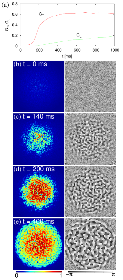
Figure 1: (a) Time evolutions of the autocorrelation functions $G_{\rm T}(t)$ and $G_{\rm L}(t)$ for sudden quench to $q=0$. (b)–(e) Snapshots of the transverse magnetization $|F_{+}(\bm{r},t)|$ (left panels) and its direction ${\rm arg}F_{+}(\bm{r},t)$ (right panels). The unit of $|F_{+}(\bm{r},t)|$ is $1.2\times 10^{14}$ ${\rm m}^{-2}$. The field of view of each panel is $400\times 400$ $\mu{\rm m}$. The number of atoms is $N=10^{7}$. See the supplementary data file for the movie showing the dynamics.

We first investigate the magnetization dynamics for sudden quench of the quadratic Zeeman energy to $q=0$. This corresponds to the situation in which the stable polar state is prepared at sufficiently large $q$, and the magnetic field is suddenly switched off at $t=0$. Figure 1(a) shows the time evolution of the autocorrelation functions $G_{\rm T}(t)$ and $G_{\rm L}(t)$. The transverse magnetization starts to grow at $t\simeq 100$ ms and the longitudinal magnetization follows. Figures 1(b)–1(e) show the profiles of the transverse magnetization. The transverse magnetization emerges around the center and grows outward. This is because the growth time in Eq. (22) is inversely proportional to the atomic density and the magnetization grows fast at which the density is large. The total density distribution $\rho(\bm{r})$ is almost unchanged during the time evolution, since $c_{0}$ is much larger than $c_{1}$.

Many spin vortices can be seen in Figs. 1(c)–1(e) (the holes in the $|F_{+}|$ profiles, around which ${\rm arg}F_{+}$ rotate by $\pm 2\pi$). In terms of the spin components in Eq. (8), $\beta$ changes by $\pm 2\pi$ around the vortex core, which is occupied by the $m=0$ component. Such a spin vortex is called a polar-core vortex. The spin winding number $w(r)$ defined in Eq. (28) represents the difference between the numbers of polar-core vortices with opposite circulations within the radius $r$.

We note that the spin vortices are produced by two distinct mechanisms in Fig. 1 with $q=0$: the KZ mechanism and the spin conservation dynamics SaitoKZ ; Saito07 . Since the spin correlation function in Eq. (II) has a finite correlation length $\xi_{\rm corr}$, the directions of magnetization at $\bm{r}$ and $\bm{r}^{\prime}$ are independent for $|\bm{r}-\bm{r}^{\prime}|\gg\xi_{\rm corr}$, giving rise to the KZ mechanism. On the other hand, when $q=0$, the total magnetization $\int\bm{F}d\bm{r}$ must be conserved at zero, since Eq. (3) is invariant with respect to spin rotation in the rotating frame $\psi_{\pm 1}\rightarrow e^{\mp ipt/\hbar}\psi_{\pm 1}$. In the present case, however, the conservation law is more strict because of the finite spin correlation length. Since the spin directions at $\bm{r}$ and $\bm{r}^{\prime}$ are independent for $|\bm{r}-\bm{r}^{\prime}|\gg\xi_{\rm corr}$, not only the total magnetization but also the local magnetization $\int_{\rm local}\bm{F}d\bm{r}$ integrated over the size of $\sim\xi_{\rm corr}$ must be conserved in each spatial region. The magnetization thus occurs in such a way that the local magnetization is conserved at zero, i.e., spin textures are formed Saito05 . Among various spin textures, the polar-core vortices are favorable, since the excess energy at the defect can be minimized Saito06 . This is the second mechanism of the spin vortex formation in Fig. 1. Thus, to see the effect of the KZ mechanism, we must take spatial region much larger than $\xi_{\rm corr}$. The correlation length is $\xi_{\rm corr}\simeq 10$ $\mu{\rm m}$ around the center of the trap and $\xi_{\rm corr}\simeq 20$ $\mu{\rm m}$ at $r=200$ $\mu{\rm m}$ for Fig. 1.

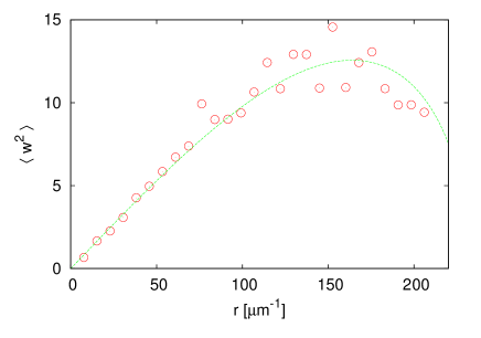
Figure 2: Variance of the winding number $\langle w^{2}(r)\rangle$ along the circumference of a circle of radius $r$ for sudden quench, where the parameters are the same as those in Fig. 1. The data for each $r$ is taken when $G_{\rm T}(r)$ exceeds 0.1. The average $\langle\cdots\rangle$ is taken over 400 runs of simulations for the different initial states produced by random numbers. The dashed curve is the least square fit of Eq. (29).

We consider the $r$-dependence of the spin winding number $w(r)$. According to the KZ theory, the number of domains along the circle of radius $r$ is $\sim r/\xi_{\rm corr}$ and hence $w^{2}(r)\sim r/\xi_{\rm corr}$. Substituting $q=0$ and $q_{\rm c}=2|c_{1}|n_{\rm TF}(r)$ into $\xi_{\rm corr}$ in Eq. (23), where $n_{\rm TF}(r)\propto R_{\rm TF}^{2}-r^{2}$ with $R_{\rm TF}$ being the Thomas–Fermi radius, we obtain

$$w^{2}(r)\propto r\sqrt{R_{\rm TF}^{2}-r^{2}}.$$ (29)

To compare Eq. (29) with the numerical simulation, we perform many runs of time evolution with different initial random noises, and take the average of $w^{2}(r)$ with respect to the runs, which is shown in Fig. 2. Since the time at which the magnetization emerges depends on $r$, each $w(r)$ is calculated when $G_{\rm T}(r)$ in Eq. (27) exceeds a certain value (0.1 in Fig. 2). The numerical result and Eq. (29) (circles and dashed curve in Fig. 2, respectively) are in good agreement, where the fitting parameter is only the proportionality coefficient in Eq. (29).

III.2 Gradual quench

We next consider the case of gradual quench of the magnetic field. The quadratic Zeeman energy $q$ is linearly decreased in the time scale $\tau_{\rm Q}$ as

$$q(t)=q_{0}(1-t/\tau_{\rm Q}),$$ (30)

for $0<t<\tau_{\rm Q}$ and $q(t)=0$ for $t\geq\tau_{\rm Q}$. As seen in the previous subsection, the critical value $q_{\rm c}(r)$ for magnetization depends on the position $r$, and $q_{0}$ is chosen to be the maximum of $q_{\rm c}(r)$. We define the time $T(r)$ at which $q$ reaches a local critical value as $q(T(r))=q_{\rm c}(r)$. The magnetization at position $r$ is expected to emerge at $t=T(r)+\Delta t(r)$ satisfying Zurek

$$\Delta t(r)\sim\tau(r,t).$$ (31)

Using Eqs. (18) and (31) with $q_{0}\Delta t(r)/[q_{\rm c}(r)\tau_{\rm Q}]\ll 1$, we obtain

$$\Delta t(r)\sim\left[\frac{\hbar^{2}}{q_{\rm c}(r)q_{0}}\right]^{1/3}\tau_{\rm Q}^{1/3}.$$ (32)

Substituting this time into Eq. (19), we obtain the $\tau_{\rm Q}$-dependence of the correlation length as

$$\xi_{\rm corr}(r)\sim\sqrt{\frac{\hbar^{2}}{Mq_{0}}}\left[\frac{q_{\rm c}(r)q_{0}}{\hbar^{2}}\right]^{1/6}\tau_{\rm Q}^{1/3}.$$ (33)

The winding number thus obeys

$$w^{2}(r)\propto\tau_{\rm Q}^{-1/3}.$$ (34)

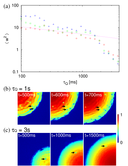
Figure 3: (a) Variance of the winding number $\langle w^{2}(r)\rangle$ along the circumference of a circle of radius $r=200$ $\mu{\rm m}$ (circles), $r=250$ $\mu{\rm m}$ (squares), and $r=300$ $\mu{\rm m}$ (triangles) for gradual quench given by Eq. (30). The data for each $r$ is taken when $G_{\rm T}(r_{\rm w})$ exceeds 0.1. The average $\langle\cdots\rangle$ is taken over 100 runs of simulations for the different initial states produced by random numbers. The dashed line is proportional to $\tau_{\rm Q}^{-1/3}$. The number of atoms is $N=10^{8}$. (b), (c) Snapshots of the transverse magnetization $|F_{+}(\bm{r},t)|$ for $\tau_{\rm Q}=$ 1 s and 3 s. The arrows trace the vortex motion. The unit of $|F_{+}(\bm{r},t)|$ is $3.4\times 10^{14}$ ${\rm m}^{-2}$. The field of view of each panel is $300\times 300$ $\mu{\rm m}$. See the supplementary data files for the movies showing the dynamics.

Figure 3 (a) shows $\langle w^{2}(r)\rangle$ obtained by numerical simulations of the GP equation (6). The variance of the winding number $\langle w^{2}(r)\rangle$ is roughly proportional to $\tau_{\rm Q}^{-1/3}$ for $100$ ${\rm ms}\lesssim\tau_{\rm Q}\lesssim 1$ s, which agrees with the above theoretical argument (34). For $\tau_{\rm Q}\lesssim 100$ ms, the assumption of $t/\tau_{\rm Q}\ll 1$ is violated; $\langle w^{2}(r)\rangle$ approaches the values for sudden quench in the limit of $\tau_{\rm Q}\rightarrow 0$. For $\tau_{\rm Q}\gtrsim 1$ s, $\langle w^{2}(r)\rangle$ significantly deviates from $\tau_{\rm Q}^{-1/3}$ and steeply drops in Fig. 3 (a). To understand this behavior, we compare the dynamics of $|F_{+}(\bm{r})|$ for $\tau_{\rm Q}=1$ s and $\tau_{\rm Q}=3$ s shown in Figs. 3(b) and 3(c). When $\tau_{\rm Q}=1$ s, new spin vortices are produced one after another as the magnetization grows outward. When $\tau_{\rm Q}=3$ s, by contrast, the spin vortex created around the center is pushed outward, and no new spin vortices are created at the front of the magnetization growth.

In the dynamics in Figs. 3(b) and 3(c), there are two characteristic velocities: the velocity $v_{\rm m}$ at which the magnetization front spreads out and the sound velocity $v_{\rm s}$ of the spin wave. The former is roughly obtained from

$$q(t)=q_{\rm c}(r_{\rm M}(t)),$$ (35)

where $r_{\rm M}(t)$ is the radius of the magnetization front. Using the Thomas–Fermi density distribution, the right-hand side is $q_{\rm c}(r_{\rm M}(t))=2|c_{1}|n_{\rm TF}(r_{\rm M}(t))\simeq q_{0}[1-r_{\rm M}^{2}(t)/R_{\rm TF}^{2}]$. The velocity $v_{\rm m}$ is thus given by

$$v_{\rm m}=\frac{dr_{\rm M}(t)}{dt}=\frac{R_{\rm TF}}{2\sqrt{\tau_{\rm Q}t}}.$$ (36)

The transverse spin wave for the broken axisymmetry state (8) is a phonon-like mode in the limit of $k\rightarrow 0$, whose velocity is given by Kawaguchi ; Murata

$$v_{\rm s}=\sqrt{\frac{q}{2M}},$$ (37)

where $q(t)$ in Eq. (30) should be used on the right-hand side. If $v_{\rm m}$ is always faster than $v_{\rm s}$, the region that is going to magnetize is causally disconnected with the magnetized region, and therefore the KZ mechanism works. It follows from Eqs. (36) and (37) that this condition is satisfied for

$$\tau_{\rm Q}<\sqrt{\frac{2M}{q_{0}}}R_{\rm TF}.$$ (38)

For the parameters in Fig. 3, the right-hand side of this inequality is $\simeq 1.7$ s, which agrees well with the time at which the plots in Fig. 3(a) deviates from $\tau_{\rm Q}^{-1/3}$.

III.3 Gradual quench with a plug potential

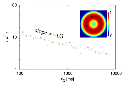
Figure 4: Variance of the winding number $\langle w^{2}(r)\rangle$ along the circumference of a circle of radius $r=250$ $\mu{\rm m}$ (dashed circle) for gradual quench given by Eq. (30). The potential has a form of Eq. (39). The data for each $r$ is taken when $G_{\rm T}(r_{\rm w})$ exceeds 0.1. The average $\langle\cdots\rangle$ is taken over 100 runs of simulations for the different initial states produced by random numbers. The dashed line is least square fit of the plots by using a function proportional to $\tau_{\rm Q}^{-1/3}$. The number of atoms is $N=10^{8}$. The inset shows the initial density profile with the unit of density $2.4\times 10^{14}$ ${\rm m}^{-2}$ and the field of view $900\times 900$ $\mu{\rm m}$.

In the previous subsection, we showed that the KZ scenario breaks down when the magnetized region expands slowly. This is because the region that is going to magnetize is causally connected to the initially magnetized region at the trap center. To eliminate this effect, we remove atoms around the trap center by adding a plug potential as

$$V_{\rm trap}(\bm{r})=\frac{1}{2}M\omega^{2}r^{2}+Ae^{-r^{2}/d^{2}},$$ (39)

where the values of the parameters are chosen to be $A=1500\hbar\omega$ and $d=222$ $\mu{\rm m}$. For these parameters, the potential $V_{\rm trap}(\bm{r})$ has a minimum at $r\simeq 250$ $\mu{\rm m}$ and the atomic density becomes maximal around this radius. As a result, the magnetization starts from the annulus around $r\simeq 250$ $\mu{\rm m}$. Therefore, magnetic domains on this radius are always causally disconnected, and the KZ mechanism is expected to work even for large $\tau_{\rm Q}$. Figure 4 shows the results of the numerical simulations. The density at $r\simeq 250$ $\mu{\rm m}$ is almost the same as the density at the same radius in the system of Fig. 3, and $\langle w^{2}(r)\rangle$ is similar to the corresponding data in Fig. 3(a) (squares) for $\tau_{\rm Q}\lesssim 1$ s. However, $\langle w^{2}(r)\rangle$ in Fig. 4 obeys the KZ scaling $\tau_{\rm Q}^{-1/3}$ even for $\tau_{\rm Q}\gtrsim 1$ s, as expected.

IV Conclusions

We have investigated the spin vortex formation due to the KZ mechanism in a quenched ferromagnetic BEC confined in a trapping potential. Since the atomic density is inhomogeneous in a harmonic trap, the spin correlation length depends on the radius $r$. In fact, the numerical simulations showed that the spin winding number depends on $r$, which was in good agreement with the theoretical prediction (Fig. 2). When the quadratic Zeeman energy $q$ is gradually quenched with the time scale $\tau_{\rm Q}$, the magnetized region gradually expands from the center to the periphery of the atomic cloud. If the expansion velocity is much faster than the spin wave velocity, the system exhibits the KZ scaling law, and if the former is slower than the latter, the KZ scenario breaks down (Fig. 3). When a plug potential is added to the harmonic trap, the geometry of the system is changed and the KZ power law can be observed over a wide range of $\tau_{\rm Q}$ (Fig. 4).

- (1) Kibble T W B 1976 J. Phys. A 9 1387
- (2) Zurek W H 1985 Nature 317 505; 1996 Phys. Rep. 276 177
- (3) Chuang I, Durrer R, Turok N, and Yurke B 1991 Science 251 1336
- (4) Bowick M J, Chandar L, Schiff E A, and Srivastava A M 1994 Science 263 943
- (5) Hendry P C, Lawson N S, Lee R A M, McClintock P V E, and Williams C D H 1994 Nature 368 315; Dodd M E, Hendry P C, Lawson N S, McClintock P V E, and Williams C D H 1998 Phys. Rev. Lett. 81 3703
- (6) Ruutu V M H, Eltsov V B, Gill A J, Kibble T W B, Krusius M, Makhlin Yu G, Plaçais B, Volovik G E, and Xu W 1996 Nature 382 334; Ruutu V M H, Eltsov V B, Krusius M, Makhlin Yu G, Plaçais B, and Volovik G E 1998 Phys. Rev. Lett. 80 1465
- (7) Bäuerle C, Bunkov Yu M, Fisher S N, Godfrin H, and Pickett G R 1996 Nature 382 332
- (8) Ducci S, Ramazza P L, González-Viñas W, and Arecchi F T 1999 Phys. Rev. Lett. 83 5210
- (9) Carmi R, Polturak E, and Koren G 2000 Phys. Rev. Lett. 84 4966
- (10) Monaco R, Mygind J, and Rivers R J 2002 Phys. Rev. Lett. 89 080603
- (11) Maniv A, Polturak E, and Koren G 2003 Phys. Rev. Lett. 91 197001
- (12) Scherer D R, Weiler C N, Neely T W, and Anderson B P 2007 Phys. Rev. Lett. 98 110402
- (13) Weiler C N, Neely T W, Scherer D R, Bradley A S, Davis M J, and Anderson B P 2008 Nature 455 948
- (14) Kawaguchi Y and Ueda M 2012 Phys. Rep. 520 253
- (15) Stamper-Kurn D M and Ueda M arXiv:1205.1888
- (16) Sadler L E, Higbie J M, Leslie S R, Vengalattore M, and Stamper-Kurn D M 2006 Nature 443 312
- (17) Leslie S R, Guzman J, Vengalattore M, Sau J D, Cohen M L, and Stamper-Kurn D M 2009 Phys. Rev. A 79 043631
- (18) Lamacraft A 2007 Phys. Rev. Lett. 98 160404
- (19) Uhlmann M, Schützhold R, and Fischer U R 2007 Phys. Rev. Lett. 99 120407
- (20) Damski B and Zurek W H 2007 Phys. Rev. Lett. 99 130402; 2008 New J. Phys. 10 045023
- (21) Saito H, Kawaguchi Y, Ueda M 2007 Phys. Rev. A 76 043613
- (22) Dziarmaga J, Meisner J, and Zurek W H 2008 Phys. Rev. Lett. 101 115701
- (23) Witkowska E, Deuar P, Gajda M, and Rzażewski K 2011 Phys. Rev. Lett. 106 135301
- (24) Sabbatini J, Zurek W H, and Davis M J 2011 Phys. Rev. Lett. 107 230402
- (25) Świsłocki T, Witkowska E, Dziarmaga J, and Matuszewski M arXiv:1208.4931
- (26) van Kempen E G M, Kokkelmans S J J M F, Heinzen D J, and Verhaar B J 2002 Phys. Rev. Lett. 88 093201
- (27) Murata K, Saito H, and Ueda M 2007 Phys. Rev. A 75 013607
- (28) Press W H, Teukolsky S A, Vetterling W T, Flannery B P 2007 Numerical Recipes, 3rd ed, Sec. 20.7 (Cambridge Univ. Press, Cambridge)
- (29) Saito H, Kawaguchi Y, and Ueda M 2007 Phys. Rev. A 75 013621
- (30) Saito H, Kawaguchi Y, and Ueda M 2005 Phys. Rev. A 72 023610
- (31) Saito H, Kawaguchi Y, and Ueda M 2006 Phys. Rev. Lett. 96 065302