The planetary spin and rotation period: A modern approach

Abstract

Using a new approach, we have obtained a formula for calculating the rotation period and radius of planets. In the ordinary gravitomagnetism the gravitational spin ($S$) orbit ($L$) coupling, $\vec{L}\cdot\vec{S}\propto L^{2}$, while our model predicts that $\vec{L}\cdot\vec{S}\propto\frac{m}{M}\,L^{2}$, where $M$ and $m$ are the central and orbiting masses, respectively. Hence, planets during their evolution exchange $L$ and $S$ until they reach a final stability at which $MS\propto mL$, or $S\propto\frac{m^{2}}{v}$, where $v$ is the orbital velocity of the planet. Rotational properties of our planetary system and exoplanets are in agreement with our predictions. The radius ($R$) and rotational period ($D$) of tidally locked planet at a distance $a$ from its star, are related by, $D^{2}\propto\sqrt{\frac{M}{m^{3}}}\,\,R^{3}$ and that $R\propto\sqrt{\frac{m}{M}}\,\,a$.

1 Introduction

Kepler’s laws best describe the dynamics of our planetary system as regards to the orbital motion. However, Newton’s law of gravitation provided the theoretical framework of these laws. In central potential the orbital angular momentum is conserved. In polar coordinates, the gravitational force consists of the ordinary attraction gravitational force and a repulsive centripetal force. The Newton’s law of gravitation has been successful in many respect. However, this law fails to account for very minute gravitational effect like deflection of light by an intervening star, precession of the perihelion of the planetary orbit and the gravitational red-shift of light passing a differential gravitational potential. Einstein’s general theory of gravitation generalizes Newton’s theory of gravitational to give a full account for all these observed gravitational phenomena. Einstein treats these phenomena as arising from the curvature of space. Hence, Einstein’s theory has become now the only accepted theory of gravitation. The inclusion of energy and momentum of matter (mass) in question leads to the curvature of space, while the inclusion of spin leads to torsion in space. Einstein’s theory deals with matter of the former case, while Einstein-Cartan deals with the latter case. Thus, Einstein space if torsion free. In classical electrodynamics the spin of a particle is a quantum effect with no classical analogue. However, the spin of a gravitating object (e.g., planets) is defined as a rotation of an object relative to its center of mass. This is expressed as $S=I\omega$, where $I$ and $\omega$ are the moment of inertia and angular velocity of the rotating object, respectively. The spin is generally a conserved quantity in physics. Besides the spin, an object ($m$) revolving at a distant $r$ around a central mass ($M$) with speed $v$ is described by its orbital angular momentum. This is defined as $L=\vec{r}\times m\vec{v}$. This quantity is also conserved, except when an external torque is acting on the object. In quantum mechanics, the spin and angular momentum of a fundamental particle are quantized. No such quantization is deemed to exist in gravitation. To incorporate quantum mechanics in gravitation we invoke a Planck-like constant characterizing every gravitational system [1, 2]. This would facilitate a bridging to quantum gravity that has not yet been uniquely formulated so far.

The spin and orbital angular momentum may couple to each other as the case in the Earth-Moon system. Therefore, neither the spin nor the orbital angular momentum are separately conserved. Their sum is always conserved. A similar coupling occurs in atomic system. For instance, because of the spin of the electron such effect is found to be present in hydrogen-like atoms.

Owing to the existing similarities between gravitation and electromagnetism, some analogies were drawn which led to gravitomagnetism paradigm. It is believed that an effect occurring in electromagnetism will have its counter analogue in gravitomagnetism.

In this paper we formulate the proper spin-orbit coupling in a gravitational system, and then deduce a formula for the spin of a gravitating object. This is done by equating the spin-orbit coupling energy to the gravitomagnetic energy. The resulting equation relates the spin of a gravitating object to its orbital angular momentum. While in standard gravitomagnetism, the gravitational spin-orbit coupling, $\vec{L}\cdot\vec{S}\propto L^{2}$, in our model of gravitomagnetism one has $\vec{L}\cdot\vec{S}\propto\frac{m}{M}\,L^{2}$. This relation suggests a balance equation, $mL\sim MS$. For this reason any orbiting object must spin in order to be dynamically stable. So planets during their course of evolution exchange $L$ and $S$, but eventually come to a state of stability. The bigger the planet the larger its spin. Hence, Jupiter spins faster than other planets in the solar system. Equivalently, the spin $S\propto\frac{Gm^{2}}{v}$, where $G$ is the gravitational constant, and $v$ is the orbital velocity. This formula is found to be consistent when applied to our planetary system and exoplanetary system. Astronomers have discovered so far more than 800 new giants planets, but couldn’t identify all of their radii and spin periods. The present formulation helps identify these latter properties. We consider here all possibilities to account for the observationally derived data pertaining to the exoplanetary system and their consistency.

2 The gravitational spin-orbit coupling

The spin - orbit interaction resulting from an interaction of the electron spin with the magnetic field arising from electron motion in hydrogen-like atom is given by

$$U_{SO}=\frac{g_{s}}{4m^{2}c^{2}r^{2}}\frac{dV}{dr}\,\vec{L}\cdot\vec{S}=-\frac{kZe^{2}}{2m^{2}c^{2}r^{3}}\vec{L}\cdot\vec{S}\,,$$ (1)

where $V=\frac{kZe^{2}}{r}$, $Z$ is the atomic number, $k$ is the Coulomb constant, $m$ is the electron mass, $c$ is the speed of light, $r$ is the radial distance of the electron from the nucleus, and $g_{s}=2$ is the gyromagnetic ratio.

In gravitomagnetism theory, we have shown that [3],

$$U_{SO-gm}=\frac{\pi g^{\prime}_{s}GM^{2}}{4m^{2}c^{2}r^{3}}\vec{L}\cdot\vec{S}\,,$$ (2)

$g\,^{\prime}_{s}$ is the gravitational gyromagnetic ratio, which corresponds to a gravitomagnetic energy

$$U_{gm}=-\frac{\pi}{3}\,\frac{GML^{2}}{2mc^{2}r^{3}}\,,$$ (3)

However, Einstein’s theory of gravitation employing Schwartzchild metric shows that because of space curvature a term of

$$U_{GR}=-\,\frac{GML^{2}}{2mc^{2}r^{3}}\,,$$ (4)

appears in the total energy of the gravitating object.

Thus, eq.(3) and (4) are very close to each other. This minute difference between the two paradigms should be further explored. Notice that the inclusion of energy momentum tensor in Einstein relativity equations leads to the space curvature, whereas the inclusion of spin would lead to the space torsion. Einstein’s general relativity respects the former but not the latter case. While Einstein attributed the precession of planets to the curvature of space, we ascribe it to the interaction of the spin of planets with the gravitomagnetic field induced by the Sun in the planet frame of reference.

Assuming the spin-orbit coupling as the one responsible for precession of perihelion of planetary orbits, the spin of a planet of mass $m$ orbiting a star of mass $M^{\prime}$ can be obtained by equating eqs.(2) and (3), i.e., spin-orbit interaction energy equals to gravitomagnetic energy, which yields

$$S=\frac{\alpha}{\cos\theta}\frac{m}{M}\,L\,,$$ (5)

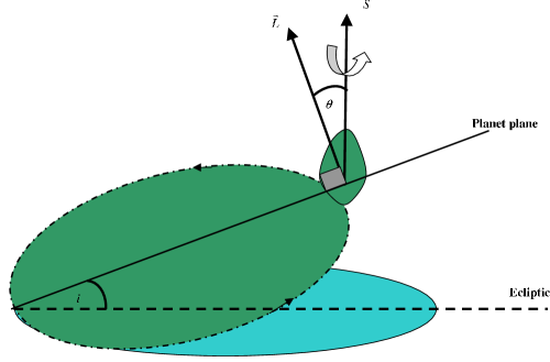
Figure 1: The inclination angle ($i$), the angle ($\theta$), the spin ($S$), and angular momentum $L$.

where $L$ is the orbital angular momentum of the orbiting planet, $\alpha=\frac{2g^{\prime}_{s}}{3}$, $\theta$ is the angle between $L$ and $S$ directions, and $M=(M^{\prime}+m)^{\dagger}$ is the total mass of the system (see figure 1). However, the orbital plane of most planets is inclined to their ecliptic with an angle ($i$). We have to decompose $L$ along the direction that is perpendicular to the ecliptic (our reference plane), hence $L\rightarrow L\cos i$ (see figure 1). Therefore, eq.(5) becomes

$$S=\alpha\frac{\cos i}{\cos\theta}\,\mu\,\,L\,,\qquad\mu=\frac{m}{M}\,.$$ (6)

Equation (6) indicates that for a system of particles each having a mass $m_{i}$, and an angular momentum $L_{i}$, the the center of mass of the angular momentum is

$$L_{C}=\frac{\Sigma_{i}\,m_{i}\,L_{i}}{\Sigma_{i}\,m_{i}}\,,$$ (7)

so that the spin could be related to a center of mass of the angular momenta of the system.

Owing to the apparent analogy between electromagnetism and gravitomagnetism, one has

$$G\rightarrow k\,,\qquad M\rightarrow Ze\,,\qquad m\rightarrow e\,,$$ (8)

so that eq.(1) would become

$$U\,^{\prime}_{SO}=\frac{g_{g}G}{4\mu\,c^{2}r^{3}}\vec{L}\cdot\vec{S}\,,$$ (9)

where $g_{g}$ is gravitational gyromagnetic ratio analogue. It is not known whether $g_{g}=2$ or not. According to the standard theory of gravitomagnetism, we can equate eqs.(4) and (9) to obtain $S=\frac{L}{\cos\theta}$ for $g_{g}=2$. This is however not correct for the planetary system. Equation (9) agrees with eq.(2) only if $g_{g}=\pi\frac{M}{m}\,g^{\prime}_{s}$.

We remark that several authors have considered the gravitational spin-orbit coupling comparing it with the atomic analogue [4, 5]. None of them have derived it from first principle, or equivalently didn’t show how the gravitational spin magnetic moment is related to the spin. This is only done in our recent publication [3]. Mashhoon proposed that the analogy between gravity and electromagnetism dictates that charge, $q\rightarrow-2m$. Hence, he concluded that the gravitational magnetic moment due to spin is related to spin by $\mu_{s}=-S$ [6]. In our gravitomagnetic theory, this is however related by the relation $\mu_{g}=\frac{M}{2m}\,S$.

Applying eq.(8) in eq.(3) dictates that the curvature term lead to a potential (interaction) energy in the atomic system

$$U_{em}=-\frac{\pi}{3}\,\frac{kZe^{2}L^{2}}{2m^{2}c^{2}r^{3}}\,.$$ (10)

Therefore, one can write the total potential energy for an electron in hydrogen-like atoms in an electric space as

$$E=-\frac{kZe^{2}}{r}+\frac{L^{2}}{2mr^{2}}-\frac{\pi}{3}\,\frac{kZe^{2}L^{2}}{2m^{2}c^{2}r^{3}}\,.$$ (11)

Comparing eqs.(1) and (10) reveals that $\vec{L}\cdot\vec{S}=\frac{\pi}{3}\,L^{2}$ for an atomic system. Thus, with this understanding the space inside an atom is not flat space (Minkowskian), but follows Schwarzschild pattern, where $\frac{2GM}{c^{2}}\rightarrow\frac{2kZe^{2}}{mc^{2}}$ is the electrical Schwarzschild radius. Hence, the metric for a spherically symmetric distribution of nuclear matter can be written as

$$ds^{2}=c^{2}(1-\frac{2kZe^{2}}{mc^{2}r})\,dt^{2}-\frac{dr^{2}}{1-\frac{2kZe^{2}}{mc^{2}r}}-r^{2}(d\theta^{2}+\sin\theta^{2}d\varphi^{2})\,.$$ (12)

One can then interpret the Rutherford-$\alpha$ deflection as a consequence of the electrical curvature inside the atom. This is tantamount to deflection of light by the Sun curvature. The electric Schwarzschild radius is equal to twice classical electron radius, $R_{s}=2r_{c}=\frac{2kZe^{2}}{mc^{2}}$. Similarly, one would expect a photon to be electrically redshifted in an electrical potential of the nucleus by an amount, $z=\frac{kZe^{2}}{mc^{2}r}$ in hydrogen-like atoms. Hence, in an analogous manner when light passe near a central charge it will experience a redshift. This can be written as, $z=\alpha\,Z\left(\frac{\lambda_{C}}{r}\right)$, where $\lambda_{C}=\frac{\hbar}{mc}$ is Compton wavelength of the electron. Now, when $r=\lambda_{C}$, then $z_{m}=\alpha\,Z$. This case represents a maximal (quantum) redshift. Thus, owing to the one-to-one analogy between gravitation and electromagnetism, one can use Einstein’s general relativity to describe electromagnetic phenomena, and Maxwell’s equation to describe gravitational phenomena.

3 The planetary spin and radius

The origin of spin of planets has not been known exactly. One can easily determine the orbital angular momentum of a planet. The spin of a planet however requires knowledge of the planet mass, radius, its rotation period and its mass distribution inside the planet. Since some planets are solid (rocky) and other are gaseous, it is not easily to identify precisely their internal structure. The former ones have generally higher rotation rate than the latter. However, orbital periods of planets depend on their distance from the Sun and the Sun mass only. We provide here a formula for spin or rotational period from its orbital motion only. Or equivalently, we relate the spin to the orbital angular momentum for the first time in history.

Equation (6) can be used to express the planetary spin as

$$S=\alpha\frac{\cos i}{\cos\theta}\,\,\frac{G\,m^{2}}{v}\,.$$ (13)

This is a very interesting and useful formula that can be used to calculate the spin of a planet without resort to its rotation period and its radius. Delauney and Flammarion related the spin period of a planet to a host of planetary physical characteristics concluding that there is a direct relationship between spin period and mean density [7]. Furthermore, Brosche noticed that some planets in a similar size range had spin angular momenta, $S$, that were proportional to the squares of their masses, $m$ [7, 8]

$$S\propto m^{2}\,.$$ (14)

Equation (14) agree partially with eq.(13). In rotational dynamics the spin of a rigid body (planet) is defined by

$$S=I\omega\,,\qquad\omega=\frac{2\pi}{D}\,,\qquad I=\lambda\,mR^{2}\,,$$ (15)

where $\lambda$ is the coefficient of inertia, $R$ the planet’s radius, and $D$ is the rotational period of the planet. Equation (13) and (15) states that the radius of the planet is

$$R=\left(\frac{\alpha\cos i}{2\pi\lambda\cos\theta}\,\frac{G\,m\,D}{v}\right)^{1/2}\,.$$ (16)

Using eqs. (6) and (15) one can write

$${\color[rgb]{0.00,0.00,1.00}\frac{D}{P}=\frac{1}{C^{2}}\,\left(\frac{R}{a}\right)^{2}\frac{1}{\mu}}\,,\qquad C=\left(\frac{\alpha\,\cos i\sqrt{1-e^{2}}}{\lambda\,\cos\,\theta}\,\right)^{1/2}\,,$$ (17)

where $P$ and $a$ are, respectively, the orbital period and the semi-major axis of the orbiting planet. Equation (17) can be written as

$${\color[rgb]{0.00,0.00,1.00}D=\frac{1}{C^{2}}\,\left(\frac{4\pi^{2}}{GM}\right)^{2/3}\left(\frac{1}{\mu}\right)\,R^{2}\,\,P^{-1/3}\,.}$$ (18)

An educated guess can relate $\alpha$ to the ellipticity (flattening/oblateness) of the planet, or to the eccentricity of the orbit. If the value of $\alpha$ is not universal for all planets, we suggest that it will depend on some geometrical factors related to a given planet. This particular relation will require more analysis that can be tackled in future work. Using eq.(15), the rotation spin rate can be written as

$$\omega=\alpha\frac{\cos i}{\cos\theta}\left(\frac{\mu\sqrt{G\,M\,a(1-e^{2})}}{\lambda\,R^{2}}\right)\,\,,$$ (19)

Equation (19) can be written as

$$\omega=\alpha\frac{\cos i}{\cos\theta}\frac{L}{I_{\lambda}}\,\,,\qquad I_{\lambda}=\lambda MR^{2}\,,\qquad L=\sqrt{G\,M\,m^{2}\,a(1-e^{2})}\,.$$ (20)

The radius of a planet that is tidally locked to its star, i.e., $P=D$, is given by (see eq.(17))

$${\color[rgb]{1.00,0.00,0.00}R_{t}=C\,\sqrt{\mu}\,\,a}\,\,.$$ (21)

Equation (18) can also be written as, for $P=D$,

$${\color[rgb]{1.00,0.00,0.00}P_{t}^{2}=C^{-3}\,\left(\frac{4\pi^{2}}{GM}\right)\left(\frac{1}{\mu}\right)^{3/2}\,R_{t}^{3}}\,.$$ (22)

It is of prime interest to mention that a hypothetical satellite that had a circular orbit radius equals to the radius of the planet, $R$, its orbital period $P$ is given by [7]

$$P_{R}^{2}=\left(\frac{4\pi}{GM}\right)\,R^{3}\,.$$ (23)

Flammarion calculated $P_{R}$ values for Earth, Jupiter, Saturn, Uranus and Neptune, by extrapolating Kepler’s Harmonic Law, as applied to their known satellites [7]. Only some of these period are in agreement with observation.

The radius of a black hole is related to its mass, $m$, by

$$R=\frac{2Gm}{c^{2}}\,.$$ (24)

Therefore, the gravitational force for such a planet (spinning black hole) is given by

$$F_{N}=\frac{G\,m\,M}{r^{2}}=C^{2}(1-e^{2})\,\frac{c^{4}}{4G}\,\frac{D}{P}\,,$$ (25)

where $r=a(1-e^{2})$. This clearly shows that a spinning black hole will experience a huge gravitational force when orbits any central massive object. It is shown by [10] that the spin of black hole ($m_{B}$) is given by $S=\chi\,Gm_{B}^{2}/c$, where $\chi$ is some constant. This agrees with eq.(13) where $v$ replaces $c$ for a black hole.

This force is maximum when the planet is tidally-locked to its star, i.e., $P=D$. Hence, one has

$$F^{\,max.}_{N}=C^{2}(1-e^{2})\frac{c^{4}}{4\,G}\,.$$ (26)

This force is of the order of $\frac{c^{4}}{G}$. It is however shown that the maximal force in nature is defined by $F_{max.}=\frac{c^{4}}{4\,G}$ [1, 2, 11]. It also represents the maximum self-gravitating mass. It is thus interesting to see that the gravitational force arising from this case is of the same order of this maximal force. For a black hole planet of radius $R_{p}$ tidally-locked with a black hole star with radius $R_{s}$, one has

$$R_{p}R_{s}=C^{2}\,a^{2}\,.$$ (27)

This is an interesting relation connecting the two radii of orbiting black that are tidally-locked to their semi major axis. Moreover, it is clear that the existence of such a system awaits the future astronomical exploration.

4 Results and discussions

We consider here the planetary system, Jupiter satellites, and Saturn satellites. The constant $C$ is calculated using eq.(18) and Tabulated in Tables 3 and 4. The average value of $C$ are 0.089, 0.077, and 0.068, for Jupiter satellites, Saturn satellites, and planetary system, respectively. Notice that for exoplanet and asteroids the constant $C$ takes the average values 7 and 0.5, respectively. The higher values of $C$ for asteroids may be attributed to the uncertainty associated with the observational data related to them. Table6 can be used to identify exoplanets that are tidally locked by comparing the values of $C$, for a given system, with that of the Moon. Since our Moon is tidally locked, and well-known, we can consider $C=0.041$ for tidally locked planets. With this value, we complete table 7. Assuming the exoplanetary system is similar to our planetary system, we suggest that $C=0.1$, as evident from table 1. With this value we calculate the day for some exoplanets as shown in table 7. Notice that Mercury is very closed to tidally-locked system envisaged in Tables 2 and 6.

5 Conclusion

Einstein’s general theory of relativity modifies the Newton’s law of gravitational by adding an extra term that Einstein attributed to the space curvature. We have shown in this work that this term could also arise from the spin-orbit interaction of spinning gravitating (planets) objects with the gravitomagnetic field. This assumption yields spin values for the planetary systems that are in agreement with observations. The equations associated with spin are then used to identify and calculate the astronomical data related to the newly discovered planets (exoplanets).

References

$[1]$ Arbab, A. I., Gen. Relativ. Gravit., 36, 2004, 2465.
$[2]$ Arbab, A. I., African J. Math. Phys., 2, 2005, 1.
$[3]$ Arbab, A. I., J. Mod. Phys., 3, 2012, 1231; Arbab, A. I., Astrophys. Space Sc., 330, 2010, 61
$[4]$ Lee, T. -Y., Physics Letters A, 291, 2001, 1.
$[5]$ Faruque, S. B., Physics Letters A, 359, 2006, 252.
$[6]$ Mashhoon, B., Physics Letters A, 173, 1993, 347.
$[7]$ Hughes, D.W., Planetary and Space Science, 51, 2003, 517.
$[8]$ Brosche, P., Icarus, 7, 1967, 132.
$[9]$ Data are obtained from http://www.wolframalpha.com, http://nssdc.gsfc.nasa.gov/planetary/factsheet/, and http://exoplanet.eu
$[10]$ Kramer, M., General Relativity with Double Pulsars, SLAC Summer Institute on Particle Physics (SSI04), Aug. 2-13, 2004, pg.1.
$[11]$ Massa, C., Astrophys. Space Sci., 232, 1995, 143.

Name	$m(\times 10^{24}\rm kg)$	$P(day)$	$D\,(hr)$	$e$	$a\,(au)$	$R\,(km)$	$C$
Mercury	0.3302	87.969	1407.6	0.2056	57.91	2439.7	0.036390953
Venus	4.8685	224.701	5832.5	0.0067	108.21	6051.8	0.009877991
Earth	5.9736	365.256	23.9345	0.0167	149.6	6378.1	0.13530133
Mars	0.64185	686.98	24.6229	0.0935	227.92	3396.2	0.195060979
Jupiter	1898.60	4332.59	9.925	0.04093	778.57	71492	0.087422946
Saturn	568.46	10759.22	10.656	0.0489	1433.53	60268	0.111249286
Uranus	86.832	30685.40	17.24	0.0565	2872.46	25559	0.079987318
Neptune	102.43	60189	16.11	0.0457	24764	4495.06	0.066062714
Pluto	0.01305	89866	153	0.244671	5874	5874	0.082682797

Table 1: The planetary system primary data

Name	$m(\times 10^{22}\rm kg)$	$a\,(\,\rm km)$	$P\,(day)$	$D(day)$	$e$	$R\,(km)$	$C$
Moon	7.3477	384400	27.321582	27.321582	0.0549	1738.14	0.041

Table 2: The Moon (tidally locked to the Earth) primary data

Name	$m(\times 10^{20}\rm kg)$	$a\,(10^{3}\,\rm km)$	$P\,(day)$	$D(day)$	$e$	$R\,(km)$	$C$
Io	893.2	421.6	1.769138	1.769138	0.004	1821.6	0.0116
Europa	480	670.9	3.551181	3.551181	0.0101	1560.8	0.0085
Ganymede	1481.9	1070.4	7.1545535	7.154553	0.0015	2631.2	0.0051
Callisto	1075.9	1882.7	16.689018	16.689018	0.007	2410.3	0.0031
Elara	0.008	11740	259.6528	0.5	0.217	40	0.0695
Himalia	0.095	11460	250.5662	0.4	0.162	85	0.0483
Metis	0.001	128	0.294779	0.294779	0.0002	20	0.3959

Table 3: Jupiter Satellites primary data

Name	$m(\times 10^{20}\rm kg)$	$a\,(10^{3}\,\rm km)$	$P\,(day)$	$D(day)$	$e$	$R\,(km)$	$C$
Miranda	0.66	129.39	1.413479	1.413479	0.0027	235.8	0.1797
Ariel	13.5	191.02	2.520379	2.520379	0.0034	578.9	0.0661
Umbriel	11.7	266.3	4.144177	4.144177	0.005	584.7	0.0514
Titania	35.2	435.91	8.705872	8.705872	0.0022	788.9	0.0244
Oberon	30.1	583.52	13.463239	13.463239	0.0008	761.4	0.0191

Table 4: Saturn Satellites (tidally locked) primary data

Name	$m(\times 10^{19}\rm kg)$	$a\,$(au)	$P\,(year)$	$D(day)$	$e$	$R\,(km)$	$C$
Ceres	87	2.767	4.6	9.075	0.0789	487.3	3.75
Juno	2	2.669	4.36	7.21	0.2579	120	6.90
Vesta	30	2.362	3.63	5.342	0.0895	265	4.71
Eugenia	0.61	2.721	4.49	5.699	0.0831	113	13.16
Siwa	0.15	2.734	4.51	18.5	0.2157	51.5	6.70
Chiron	0.4	13.633	50	5.9	0.3801	90	8.48
Haumea	41.79	43.335	285.4	3.912	0.18874	718	6.11
Pallas	3.18	2.7707	3.62	7.8132	0.231	261	10.03
Eris	1.62	2.385	3.68	7.14	0.231	199.8	13.18

Table 5: Asteroids primary data

Name	$m(M_{J})$	$M(M_{\odot})$	$a\,$(au)	$R(R_{J})$	$P(day)$	$C$
Kepler-34(AB) b	0.22	2.0687	1.0896	0.76	288.822	0.0350
Kepler-9 c	0.171	1	0.225	0.823	38.9086	0.0395
KOI-55 c	0.0021	0.496	0.0076	0.078	0.34289	0.0395
HD 97658 b	0.02	0.85	0.0797	0.262	9.4957	0.0329
GJ 3470 b	0.044	0.541	0.0348	0.376	3.33714	0.0453
Kepler-22b	0.11	0.97	0.85	0.214	289.9	0.0425
Gl 581 g	0.01	0.31	0.14601	0.0678	36.652	0.0429

Table 6: Tidally-locked Exoplanets primary data [9]

Name	$m(M_{J})$	$M(M_{\odot})$	$a\,$(au)	$P\,(day)$	$R(R_{J})$	$D(day)$
WASP-10 b	3.06	0.71	0.0371	3.09276	1.08	0.6566
XO-5 b	1.077	0.88	0.0487	4.18775	1.03	0.4783
WASP-16 b	0.855	1.022	0.042	3.1186	1.008	0.1891
KOI-204 b	1.02	1.19	0.0455	3.24674	1.24	0.1564
XO-2 b	0.62	0.98	0.0369	2.61584	0.973	0.0993
TrES-1	0.761	0.88	0.0393	3.03007	1.099	0.1398
WASP-1 b	0.86	1.24	0.0382	2.51995	1.484	0.0483
HAT-P-17 b	0.534	0.857	0.0882	10.3385	1.01	2.051
WASP-55 b	0.57	1.01	0.0533	4.46563	1.3	0.1768
WASP-6 b	0.503	0.888	0.0421	3.36101	1.224	0.0940
55 Cnc e	0.0263	0.905	0.0156	0.736546	0.194	0.00578
OGLE2-TR-L9 b	4.34	1.52	0.0308	2.48553	1.614	0.1079
OGLE-TR-10 b	0.68	1.18	0.04162	3.10129	1.72	0.04368
XO-3 b	11.79	1.213	0.0454	3.19152	1.217	1.802
PSR 1719-14 b	1	1.4	0.0044	0.0907063	0.4	0.000327
WASP-14 b	7.341	1.211	0.036	2.24377	1.281	0.4484
HD 80606 b	3.94	0.98	0.449	111.436	0.921	4444.9

Table 7: Some non-tidally locked Exoplanets primary data [9]. The day is obtained for $C=0.1$ as can be guessed from table 2 for planetary system.