Two-Way Training for Discriminatory Channel Estimation in Wireless MIMO Systems

Abstract

This work examines the use of two-way training to efficiently discriminate the channel estimation performances at a legitimate receiver (LR) and an unauthorized receiver (UR) in a multiple-input multiple-output (MIMO) wireless system. This work improves upon the original discriminatory channel estimation (DCE) scheme proposed by Chang et al where multiple stages of feedback and retraining were used. While most studies on physical layer secrecy are under the information-theoretic framework and focus directly on the data transmission phase, studies on DCE focus on the training phase and aim to provide a practical signal processing technique to discriminate between the channel estimation performances (and, thus, the effective received signal qualities) at LR and UR. A key feature of DCE designs is the insertion of artificial noise (AN) in the training signal to degrade the channel estimation performance at UR. To do so, AN must be placed in a carefully chosen subspace based on the transmitter’s knowledge of LR’s channel in order to minimize its effect on LR. In this paper, we adopt the idea of two-way training that allows both the transmitter and LR to send training signals to facilitate channel estimation at both ends. Both reciprocal and non-reciprocal channels are considered and a two-way DCE scheme is proposed for each scenario. For mathematical tractability, we assume that all terminals employ the linear minimum mean square error criterion for channel estimation. Based on the mean square error (MSE) of the channel estimates at all terminals, we formulate and solve an optimization problem where the optimal power allocation between the training signal and AN is found by minimizing the MSE of LR’s channel estimate subject to a constraint on the MSE achievable at UR. Numerical results show that the proposed DCE schemes can effectively discriminate between the channel estimation and hence the data detection performances at LR and UR.

Index terms$-$ Two-way training, Channel estimation, Physical layer secrecy, MIMO

I Introduction

Due to the broadcast nature of the wireless medium, communication between wireless terminals is often susceptible to potential eavesdropping by unauthorized receivers. Therefore, as wireless technology becomes more prevalent, the need for discriminating between the signal reception performance at a legitimate receiver (LR) and that at an unauthorized receiver (UR) has increased. Motivated by this demand, the concept of physical layer secrecy have been studied extensively in recent years and methods that utilize properties of the wireless channels to achieve the desired performance discrimination have been proposed. From an information-theoretic viewpoint, the difference in the channel condition at different receivers can be exploited to ensure a non-zero communication rate between the transmitter and LR under the perfect secrecy constraint [1, 2, 3, 4], where the notion of perfect secrecy means that no UR is able to infer any information from the received signal broadcasted by the transmitter. From a signal processing perspective, artificial-noise-aided multiuser beamforming schemes [5, 6, 7] and space-time coding schemes [8] can be adopted to enhance signal reception at LR while limiting the received signal quality at UR.

I-A Motivation and Related Work

Most studies in the literature on physical layer secrecy, e.g., [1, 2, 3, 4, 5, 6, 7, 8], focus on the design of the data transmission phase while often assuming the availability of perfect channel state information. In practice, channel knowledge is typically obtained through training and channel estimation, and its quality can have a significant impact on the receiver performance [9, 10]. Intuitively, if UR has a poorer channel estimation performance than LR, then UR would have a higher detection error probability when overhearing the transmission of secret messages. Motivated by this observation, the authors in [11] proposed a novel training scheme, called discriminatory channel estimation (DCE), that can provide a better channel estimation performance for LR compared to that for UR. Different from the information-theoretic works [1, 2, 3], the DCE scheme in [11] takes a more practical viewpoint and is a signal processing technique for discriminating between the channel conditions of LR and UR.

The key feature of the DCE scheme [11] is the insertion of artificial noise (AN) in the training signal. The AN is carefully placed in a subspace so that it jams UR while the interference caused to LR is minimized. To this end, the transmitter requires knowledge of LR’s channel. In the original DCE scheme proposed in [11], this was achieved by using a preliminary training stage followed by multiple stages of feedback-and-retraining. Specifically, in the preliminary training stage, a pure pilot signal is first sent by the transmitter to allow for a rough channel estimate at LR. Then, LR feeds back this channel estimate to the transmitter, who then sends a new pilot signal inserted with AN to disrupt the channel estimation at UR. The pilot signal power used in the preliminary training stage must be relatively small since, otherwise, UR is also able to obtain a good channel estimate. In addition, the AN signal used in the retraining stage must be placed in the null-space of LR’s estimated channel to minimize its effect on LR. Through each stage of feedback and retraining, knowledge of LR’s channel at the transmitter is gradually refined, allowing AN to be placed more precisely in the desired signal subspace and the pilot signal power to be increased without benefiting the channel estimation at UR. The main drawback of this multi-stage feedback-and-retraining scheme [11] is the large training overhead and the high design complexity required. The cost and the quality of the feedback link may also limit its application in practice, but was not considered in [11].

I-B Our Approach and Contribution

The main contribution of this work is to propose new and efficient DCE schemes based on the two-way training methodology. The idea of two-way training, which has been studied for non-secrecy applications, e.g., in [19, 20, 21, 22, 23, 24], allows both the transmitter and the receiver to send pilot signals in a collaborative manner so that channel estimation is enabled at both ends. This is particularly useful in achieving DCE since the reverse training signal sent by LR in a two-way training scheme will not benefit UR in obtaining any information about the channel between itself and the transmitter. This advantage is not enjoyed by conventional one-way training schemes since any pilot signal sent by the transmitter will help UR improve its estimate of the channel between itself and the transmitter. In this work, two-way DCE schemes are designed for both reciprocal and non-reciprocal channel models. The former is a reasonable model for time-division duplex (TDD) systems whereas the latter is often used to model frequency-division duplex (FDD) systems. For reciprocal channels, the proposed two-way DCE scheme requires only two stages of training, that is, a reverse training stage and a forward training stage. For non-reciprocal channels, only an additional round-trip training stage is needed, in which the transmitter first broadcasts a random signal only known to itself and LR echoes the signal back using an amplify-and-forward strategy. In both cases, AN is inserted into the pilot signal in the (final) forward training stage to achieve the desired DCE performance. Compared to the multi-stage feedback-and-retraining scheme proposed in [11], the newly proposed two-way training schemes drastically reduce the overall training overhead.

The proposed two-way DCE schemes can conceptually be derived under any channel estimation criterion at the three terminals. For tractability and for gaining useful insights, in this paper, we assume that all terminals employ the linear minimum mean square error (LMMSE) channel estimator, and derive the resulting mean square error (MSE) of the channel estimates obtained at both LR and UR. These analysis results are then used to compute the optimal power allocation between the pilot signals and AN across different training stages. This is obtained by solving an optimization problem that aims to minimize the MSE of LR’s channel estimate subject to a constraint on the MSE of UR’s channel estimate and individual training energy constraints at the transmitter and LR. For reciprocal channels, we show that the optimal transmit powers of reverse training, forward training, and AN have simple close-form expressions. For non-reciprocal channels, the power allocation problem cannot be easily solved, but an approximate solution can be obtained by employing the monomial approximation and the condensation method [25, 26] often used in the field of geometric programming (GP). Numerical results are provided to demonstrate the effectiveness of the proposed schemes.

The remainder of this paper is organized as follows. In Section II, the system model and the proposed two-way DCE scheme for reciprocal channels are presented. In Section III, the two-way DCE scheme is extended to non-reciprocal channels. Numerical results are provided in Section IV and, finally, the conclusion is given in Section V.

Notations: Upper-case and lower-case boldfaced letters are used for matrices, e.g., $\mathbf{X}$, and vectors, e.g., $\mathbf{x}$, respectively. Moreover, $\mathbf{X}^{T}$, $\mathbf{X}^{*}$ and $\mathbf{X}^{H}$ denote the transpose, the complex conjugate and the Hermitian of the matrix $\mathbf{X}$, respectively. Let $\mathbf{0}_{M\times N}$ be the $M$-by-$N$ zero matrix and let $\mathbf{I}_{M}$ be the $M$-by-$M$ identity matrix. $\mbox{Tr}(\cdot)$ denotes the trace of a square matrix, $\|\cdot\|$ denotes the Frobenius norm, and $\mbox{vec}(\cdot)$ is the operator which stacks the columns of a matrix into a vector. The symbol $\otimes$ denotes the Kronecker matrix product, $\mathbb{E}\{\cdot\}$ denotes the expectation operator and ${\rm diag}(a_{1},\dots,a_{N})$ is the $N\times N$ diagonal matrix with diagonal elements $a_{1},\dots,a_{N}$.

II Two-Way DCE Design for Reciprocal Channels

II-A System Model

Consider a wireless MIMO system that consists of a transmitter, a legitimate receiver (LR), and an unauthorized receiver (UR), which are equipped with ${N_{t}}$, $N_{L}$ and $N_{U}$ antennas, respectively, as shown in Fig. 1. We assume that ${N_{t}}>{N_{L}}$. Moreover, the channel fading coefficients are assumed to remain constant during each transmission block, which consists of a training phase and a data transmission phase. In this work, we focus on the training phase and aim to discriminate the channel estimation performances at LR and UR. Let the downlink channel matrix from the transmitter to LR be denoted by ${\mathbf{H}_{d}}\in\mathbb{C}^{{N_{t}}\times{N_{L}}}$. The entries of ${\mathbf{H}_{d}}$ are assumed to be independent and identically distributed (i.i.d.) complex Gaussian random variables with zero mean and variance $\sigma_{h_{d}}^{2}$ (i.e., ${\mathcal{C}}{\mathcal{N}}(0,\sigma_{h_{d}}^{2})$). Similarly, the uplink channel from LR to the transmitter is denoted by ${\mathbf{H}_{u}}\in\mathbb{C}^{{N_{L}}\times{N_{t}}}$, whose entries are i.i.d. with distribution ${\mathcal{C}}{\mathcal{N}}(0,\sigma_{h_{u}}^{2})$. The forward channel from the transmitter to UR is denoted by ${\mathbf{G}}\in\mathbb{C}^{{N_{t}}\times{N_{U}}}$ with entries being i.i.d. ${\mathcal{C}}{\mathcal{N}}(0,\sigma_{g}^{2})$; while the channel from LR to UR is denoted by ${\mathbf{F}}\in\mathbb{C}^{{N_{L}}\times{N_{U}}}$. In the rest of the paper, we assume that the transmitter, LR and UR are separated enough so that ${\mathbf{H}_{d}}$ (${\mathbf{H}_{u}}$), ${\mathbf{G}}$ and ${\mathbf{F}}$ are distinct and statistically independent of each other.

In the case of reciprocal channels, the uplink and downlink channel matrices can be specified by a single channel matrix ${\mathbf{H}}$ such that ${\mathbf{H}}\triangleq{\mathbf{H}_{d}}=\mathbf{H}^{T}_{u}\in\mathbb{C}^{{N_{t}}\times N_{L}}$. The variance of each entry can be denoted by ${\sigma_{h}^{2}}$, where ${\sigma_{h}^{2}}=\sigma_{h_{d}}^{2}=\sigma_{h_{u}}^{2}$. With such channel reciprocity, the transmitter can obtain an estimate of the downlink channel by taking the transpose of the estimated channel matrix obtained through reverse training, i.e., training based on the pilot signals sent from LR to the transmitter. In the following subsections, we show the detailed steps of the proposed two-way DCE scheme and the associated LMMSE channel estimation performance in reciprocal channels.

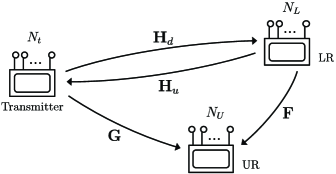
Figure 1: A wireless MIMO system consisting of a transmitter, a legitimate receiver (LR) and an unauthorized receiver (UR).

II-B Training Scheme and Channel Estimation Performance

Step I (Channel Acquisition at Transmitter via Reverse Training): The first step of the two-way DCE scheme is to allow the transmitter to obtain a reliable estimate of its downlink channel to LR without benefiting the channel estimation process at UR. Different from [11], where the availability of a noiseless feedback link was considered, our proposed two-way DCE scheme requires the transmitter to estimate the downlink channel by itself through the exchange of training signals between the transmitter and LR. In the reciprocal channel case, this can be simply achieved by having LR send a reverse training signal to the transmitter. Specifically, in the reverse training stage, LR first sends a training signal

$${\mathbf{X}}_{L}=\sqrt{\frac{\mathcal{P}_{R}\tau_{R}}{N_{L}}}{\mathbf{C}}_{L}$$ (1)

to the transmitter, where ${\mathbf{C}}_{L}\in\mathbb{C}^{\tau_{R}\times{N_{L}}}$ is the pilot matrix that satisfies ${\mathbf{C}}^{H}_{L}{\mathbf{C}}_{L}=\mathbf{I}_{N_{L}}$, $\mathcal{P}_{R}$ is the transmission power for reverse training, and $\tau_{R}$ is the reverse training length. Note that the choice of using an orthonormal pilot matrix (i.e., ${\mathbf{C}}^{H}_{L}{\mathbf{C}}_{L}=\mathbf{I}_{N_{L}}$) is due to its optimality in minimizing the channel estimation error in point-to-point channels, as shown in [10]. In the remainder of this paper, we shall sometimes denote the reverse training energy by $\mathcal{E}_{R}$ while keeping in mind that

$${\mathcal{E}_{R}\triangleq\mathcal{P}_{R}\tau_{R}.}$$

The signal received at the transmitter is given by

$$\mathbf{Y}_{t}={\mathbf{X}}_{L}{\mathbf{H}}^{T}+\widetilde{\mathbf{W}},$$ (2)

where $\widetilde{\mathbf{W}}\in\mathbb{C}^{\tau_{R}\times{N_{t}}}$ is the AWGN matrix with elements being i.i.d. $\mathcal{CN}(0,\sigma_{\tilde{w}}^{2})$.

The reverse training signal sent by LR allows the transmitter to obtain an estimate of the downlink channel by taking the transpose of its uplink channel estimate. By employing the LMMSE estimator [27], the estimate of ${\mathbf{H}}$ at the transmitter can be written as

$$\widehat{\mathbf{H}}=\left({\sigma_{h}^{2}}\mathbf{X}_{L}^{H}({\sigma_{h}^{2}}\mathbf{X}_{L}\mathbf{X}_{L}^{H}+\sigma_{\tilde{w}}^{2}\mathbf{I}_{\tau_{R}})^{-1}\mathbf{Y}_{t}\right)^{T}\triangleq{\mathbf{H}}+\Delta{\mathbf{H}}$$ (3)

where $\Delta{\mathbf{H}}\in\mathbb{C}^{{N_{t}}\times{N_{L}}}$ is the estimation error matrix with

$$\mathbb{E}\{\Delta{\mathbf{H}}(\Delta{\mathbf{H}})^{H}\} ={N_{L}}\left(\frac{1}{\sigma_{h}^{2}}+\frac{\mathcal{E}_{R}}{N_{L}\sigma_{\tilde{w}}^{2}}\right)^{-1}\mathbf{I}_{{N_{t}}},$$ (4)

and $\sigma_{\tilde{w}}^{2}$ is the noise power at the transmitter.

Step II (Forward Training with AN): After obtaining the downlink channel estimate, i.e., $\widehat{{\mathbf{H}}}$, in Step I, the transmitter then sends a forward training signal to enable channel estimation at LR in Step II. To degrade the channel estimation performance of UR while not jamming LR, the transmitter carefully inserts AN in the training signal. The forward training signal is given by

$${{\mathbf{X}}_{t}=\sqrt{\frac{\mathcal{P}_{F}\tau_{F}}{{N_{t}}}}{\mathbf{C}}_{t}+{\mathbf{A}}\mathbf{K}_{\widehat{{\mathbf{H}}}}^{H}},$$ (5)

where ${\mathbf{C}}_{t}\in\mathbb{C}^{\tau_{F}\times{N_{t}}}$ is the pilot matrix with $\text{Tr}({\mathbf{C}}_{t}^{H}{\mathbf{C}}_{t})={N_{t}}$, $\mathcal{P}_{F}$ is the pilot signal power in this stage, and $\tau_{F}$ is the training length. For ease of notation, we define

$$\mathcal{E}_{F}\triangleq\mathcal{P}_{F}\tau_{F}$$

as the forward pilot signal energy. Here ${\mathbf{A}}\in\mathbb{C}^{\tau_{F}\times({N_{t}}-{N_{L}})}$ is AN matrix whose entries are i.i.d. $\mathcal{CN}(0,{\sigma_{a}^{2}})$ and are statistically independent of the channels and noises at all terminals; $\mathbf{K}_{\widehat{{\mathbf{H}}}}\in\mathbb{C}^{{N_{t}}\times({N_{t}}-{N_{L}})}$ is a matrix whose column vectors form an orthonormal basis for the left null space of $\widehat{{\mathbf{H}}}$, that is, $\mathbf{K}_{\widehat{{\mathbf{H}}}}^{H}\widehat{{\mathbf{H}}}=\mathbf{0}_{({N_{t}}-{N_{L}})\times{N_{L}}}$ and $\mathbf{K}_{\widehat{{\mathbf{H}}}}^{H}\mathbf{K}_{\widehat{{\mathbf{H}}}}=\mathbf{I}_{{N_{t}}-{N_{L}}}$. Notice from (5) that AN is superimposed on the training signal and placed in the left null space of $\widehat{{\bf H}}$ to minimize its interference on LR. The received signals at LR and UR are respectively given by

$$\mathbf{Y}_{L} =\sqrt{\frac{\mathcal{E}_{F}}{{N_{t}}}}{\mathbf{C}}_{t}{\mathbf{H}}+{\mathbf{A}}\mathbf{K}_{\widehat{{\mathbf{H}}}}^{H}{\mathbf{H}}+\mathbf{W},$$ (6)

$$\mathbf{Y}_{U} =\sqrt{\frac{\mathcal{E}_{F}}{{N_{t}}}}{\mathbf{C}}_{t}{\mathbf{G}}+{\mathbf{A}}\mathbf{K}_{\widehat{{\mathbf{H}}}}^{H}{\mathbf{G}}+{\mathbf{V}},$$ (7)

where $\mathbf{W}\in\mathbb{C}^{\tau_{F}\times{N_{L}}}$ and ${\mathbf{V}}\in\mathbb{C}^{\tau_{F}\times{N_{U}}}$ are the additive white Gaussian noise (AWGN) matrices at LR and UR, respectively, with entries being i.i.d. ${\mathcal{C}}{\mathcal{N}}(0,\sigma_{w}^{2})$ and ${\mathcal{C}}{\mathcal{N}}(0,{\sigma_{v}^{2}})$, respectively. Note that, since $\widehat{\mathbf{H}}={\mathbf{H}}+\Delta{\mathbf{H}}$ and $\mathbf{K}_{\widehat{{\mathbf{H}}}}^{H}\mathbf{\widehat{H}}=\mathbf{0}$, equation (6) can be rewritten as

$$\mathbf{Y}_{L} =\sqrt{\frac{\mathcal{E}_{F}}{{N_{t}}}}{\mathbf{C}}_{t}{\mathbf{H}}-{\mathbf{A}}\mathbf{K}_{\widehat{{\mathbf{H}}}}^{H}\Delta{\mathbf{H}}+\mathbf{W}\triangleq\bar{\mathbf{C}}{\mathbf{H}}+\bar{\mathbf{W}},$$ (8)

where $\bar{\mathbf{C}}\triangleq\sqrt{\frac{\mathcal{E}_{F}}{{N_{t}}}}{\mathbf{C}}_{t}$ and $\bar{\mathbf{W}}\triangleq-{\mathbf{A}}\mathbf{K}_{\widehat{{\mathbf{H}}}}^{H}\Delta{{\mathbf{H}}}+\mathbf{W}$. Also note that, due to the presence of ${\bf A}$, $\bar{\mathbf{W}}$ is statistically uncorrelated with ${\mathbf{H}}$, i.e., ${\rm E}\{\bar{\mathbf{W}}^{H}{\bf H}\}={\bf 0}$.

By assuming the LMMSE estimator, the channel estimate at LR can be expressed as

$$\widehat{\mathbf{H}}_{L}={\mathbf{R}}_{{\mathbf{H}}}{\bar{\mathbf{C}}}^{H}(\bar{\mathbf{C}}{\mathbf{R}}_{{\mathbf{H}}}{\bar{\mathbf{C}}}^{H}+{\mathbf{R}}_{\bar{\mathbf{W}}})^{-1}\mathbf{Y}_{L},$$ (9)

where $\mathbf{R}_{\mathbf{H}}=\mathbb{E}\{{\mathbf{H}}{\mathbf{H}}^{H}\}={N_{L}}\sigma_{h}^{2}\mathbf{I}_{{N_{t}}}$ and $\mathbf{R}_{\bar{\mathbf{W}}}=\mathbb{E}\{\bar{\mathbf{W}}{\bar{\mathbf{W}}}^{H}\}$. The normalized mean squared error (NMSE) of $\mathbf{\widehat{H}}_{L}$ is defined as

$$\mbox{NMSE}_{L} \triangleq\frac{\mbox{Tr}\left(\mathbb{E}\{({\mathbf{H}}-\mathbf{\widehat{H}}_{L})({\mathbf{H}}-\mathbf{\widehat{H}}_{L})^{H}\}\right)}{{N_{t}}{N_{L}}}$$

$$=\frac{\mbox{Tr}\left(\left(\mathbf{R}_{\mathbf{H}}^{-1}+\bar{\mathbf{C}}^{H}\mathbf{R}_{\bar{\mathbf{W}}}^{-1}\bar{\mathbf{C}}\right)^{-1}\right)}{{N_{t}}{N_{L}}}.$$ (10)

By the fact that $\hat{\mathbf{H}}$ and $\Delta{\mathbf{H}}$ are uncorrelated due to the orthogonality principle [27], and by (4) and $\mathbf{K}_{\widehat{{\mathbf{H}}}}^{H}\mathbf{K}_{\widehat{{\mathbf{H}}}}=\mathbf{I}_{{N_{t}}-{N_{L}}}$, the covariance of $\bar{\mathbf{W}}$ can be written as

$$\mathbf{R}_{\bar{\bf W}} =\left(\mathbb{E}\{\lVert\mathbf{K}_{\widehat{H}}^{H}\Delta{\mathbf{H}}\rVert^{2}\}\sigma_{a}^{2}+{N_{L}}\sigma_{w}^{2}\right)\mathbf{I}_{\tau_{F}}$$

$$={N_{L}}\left[({N_{t}}-{N_{L}})\cdot\left(\frac{1}{\sigma_{H}^{2}}+\frac{\mathcal{E}_{R}}{{N_{L}}\sigma_{\tilde{w}}^{2}}\right)^{-1}\sigma_{a}^{2}+\sigma_{w}^{2}\right]\mathbf{I}_{\tau_{F}}.$$ (11)

Then, by substituting (11) into (II-B), we have

$$\mbox{NMSE}_{L}=\frac{1}{{N_{t}}}\mbox{Tr}\bigg{(}\bigg{(}\frac{1}{\sigma_{h}^{2}}\mathbf{I}_{{N_{t}}}+$$

$$~{}~{}~{}~{}~{}~{}~{}\frac{\mathcal{E}_{F}}{{N_{t}}}\frac{{\mathbf{C}}^{H}_{t}{\mathbf{C}}_{t}}{({N_{t}}-{N_{L}})\bigg{(}\frac{1}{\sigma_{h}^{2}}+\frac{\mathcal{E}_{R}}{{N_{L}}\sigma_{\tilde{w}}^{2}}\bigg{)}^{-1}\sigma_{a}^{2}+\sigma_{w}^{2}}\bigg{)}^{\!\!\!\!-1}\bigg{)}.$$ (12)

Similarly, the NMSE of the estimate of ${\mathbf{G}}$ at UR can be computed as

$$\mbox{NMSE}_{U}=$$

$$~{}~{}\frac{1}{{N_{t}}}\mbox{Tr}\left(\left(\frac{1}{\sigma_{g}^{2}}\mathbf{I}_{{N_{t}}}+\frac{\mathcal{E}_{F}}{{N_{t}}}\frac{\mathbf{C}^{H}_{t}{\mathbf{C}}_{t}}{({N_{t}}-{N_{L}})\sigma_{a}^{2}\sigma_{g}^{2}+\sigma_{v}^{2}}\right)^{-1}\right).$$ (13)

Notice, from (II-B) and (II-B), that increasing the AN power (i.e., ${\sigma_{a}^{2}}$) increases the NMSE at both receivers, but the effect can be reduced at LR by increasing the reverse training energy $\mathcal{E}_{R}$. Hence, under a total energy constraint, the training and AN powers must be carefully chosen to ensure sufficient discrimination between the channel estimation performances at the two receivers.

Remark 1.

In view of the fact that the proposed forward training signal in (5) contains AN, an important question to ask is that whether UR can ignore the AN-aided training signal and directly employ some blind data detection or channel estimation methods in the data transmission phase. For example, if the transmitter uses space-time coding schemes in the data transmission phase, UR may employ the blind detection methods in [12, 13, 14] or the blind channel estimation methods in [15, 16]. However, these blind methods cannot work properly without cooperation of the transmitter. Specifically, if the transmitter uses space-time codes that are not identifiable [16, 17], UR would suffer from nontrivial code and channel rotation ambiguities. It has been shown in [18] that the rotation ambiguities can make UR have a detection error probability equal to one, provided that the information symbols satisfy a constant modulus property. As a result, UR may still need to exploit the training signal for channel estimation, even though it is jammed by the AN signal. Further quantitative analysis evaluating the performance of other data transmission schemes and blind detection/channel estimation methods under the proposed DCE scheme will be an interesting direction for future research.

II-C Optimal Power Allocation between Pilot Signal and AN

The closed-form NMSE expressions obtained in the previous subsection show explicitly the effect of the reverse training power (or energy), the forward training power (or energy) and the AN power on the channel estimation performances at LR and UR. From a designer’s point of view, it is desirable to utilize the available power (or energy) in an efficient way whilst achieving a satisfactory DCE performance. In the following, we consider the problem of allocating the pilot signal and AN powers in the reverse and forward training stages with the goal of minimizing the channel estimation error at the LR whilst keeping the estimation error at UR above a certain threshold. The proposed optimization problem is given as follows:

$$\min_{\mathcal{E}_{R},\mathcal{E}_{F},\sigma_{a}^{2}\geq 0} \mbox{NMSE}_{L}$$ (14a)

subject to (s.t.) $$\mbox{NMSE}_{U}\geq\gamma,$$ (14b)

$$\mathcal{E}_{R}\leq\bar{\mathcal{E}}_{L},$$ (14c)

$$\mathcal{E}_{F}+({N_{t}}-{N_{L}})\sigma_{a}^{2}\tau_{F}\leq\bar{\mathcal{E}}_{t}.$$ (14d)

The optimization problem is constrained by a required lower limit on UR’s NMSE in (14b), and individual energy constraints at LR and the transmitter in (14c) and (14d), respectively.

It should be noted that UR’s NMSE constraint, i.e., $\gamma$, [11] should be chosen such that

$${\left(\frac{1}{\sigma_{g}^{2}}+\frac{\bar{\mathcal{E}}_{t}}{{N_{t}}\sigma_{v}^{2}}\right)^{-1}\leq\gamma\leq\sigma_{g}^{2},}$$ (15)

where the term on the left hand side is the minimum achievable NMSE at UR (when the transmitter does not use any AN, i.e., $\sigma_{a}^{2}=0$) and the term on the right hand side stands for the worst NMSE performance at UR (which is achieved when the mean of ${\bf G}$, i.e., zero, is taken as the channel estimate). For ease of use later, let us define

$${\tilde{\gamma}}\triangleq\left(\frac{1}{\gamma}-\frac{1}{\sigma_{g}^{2}}\right){N_{t}}\sigma_{v}^{2}\geq 0$$ (16)

so that the condition in (15) can be reduced to

$$0\leq{\tilde{\gamma}}\leq\bar{\mathcal{E}}_{t}.$$ (17)

The power allocation problem in (14) is a non-convex optimization problem involving three variables ($\mathcal{E}_{R},\mathcal{E}_{F},\sigma_{a}^{2}$). Interestingly, we show in the following proposition that, for the case of orthogonal forward pilot matrices (i.e., the case where ${\mathbf{C}}_{t}^{H}{\mathbf{C}}_{t}=\mathbf{I}_{{N_{t}}}$), problem (14) actually has simple closed-form solutions.

Proposition 1.

Consider problem (14) with $\gamma$ chosen according to (15). If

$$\mu\triangleq{N_{L}}\left(\frac{\sigma_{v}^{2}\sigma_{\tilde{w}}^{2}}{\sigma_{g}^{2}\sigma_{w}^{2}}-\frac{\sigma_{\tilde{w}}^{2}}{\sigma_{h}^{2}}\right)>\bar{\mathcal{E}}_{L},$$ (18)

the optimal $(\mathcal{E}_{R},\mathcal{E}_{F},{\sigma_{a}^{2}})$ is given by $\mathcal{E}_{R}^{\star}=0$, $\mathcal{E}_{F}^{\star}={\tilde{\gamma}}$ and $({\sigma_{a}^{2}})^{\star}=0$ (i.e., no need of reverse training and AN). On the other hand, if $\mu\leq\bar{\mathcal{E}}_{L}$, the transmitter and LR use all the available energy so that $\mathcal{E}^{\star}_{R}=\bar{\mathcal{E}}_{L}$,

$$\mathcal{E}^{\star}_{F}=\bar{\mathcal{E}}_{t}-\frac{(\bar{\mathcal{E}}_{t}-{\tilde{\gamma}})\tau_{F}}{\tau_{F}+{\tilde{\gamma}}\sigma_{g}^{2}/{\sigma_{v}^{2}}},$$

and

$$({\sigma_{a}^{2}})^{\star}=\frac{\bar{\mathcal{E}}_{t}-{\tilde{\gamma}}}{\left(\tau_{F}+{\tilde{\gamma}}\sigma_{g}^{2}/{\sigma_{v}^{2}}\right)({N_{t}}-{N_{L}})}.$$

Proposition 1 implies that, if UR has a relatively poor channel condition (i.e., sufficiently small ${\sigma_{g}^{2}}/{\sigma_{v}^{2}}$), then both AN and reverse training are not needed; otherwise, LR should use all its energy for reverse training and the transmitter needs to employ AN in order to constrain UR’s MSE above the required threshold value $\gamma$. The proof of Proposition 1 is given in Appendix A. Appendix A actually provides the proof for a more general formulation which, compared to problem (14), has an additional total energy constraint

$$\mathcal{E}_{R}+\mathcal{E}_{F}+({N_{t}}-{N_{L}})\sigma_{a}^{2}\tau_{F}\leq\bar{\mathcal{E}}_{tot},$$

where $\bar{\mathcal{E}}_{tot}$ represents the total energy budget. This total energy constraint limits the total amount of energy consumed by the transmitter and LR in the training phase. We are interested in such general formulation because it may be useful in the system design stage for understanding the power tradeoff between the transmitter and LR and that between the training phase and data transmission phase.

Two remarks regarding the proposed DCE scheme are in order.

Remark 2.

It is interesting to note that Proposition 1 gives the solution to the optimization problem for the orthogonal forward training matrix with full rank, i.e., ${\mathbf{C}}^{H}_{t}{\mathbf{C}}_{t}=\mathbf{I}_{{N_{t}}}$. However, the rank of ${\mathbf{C}}_{t}$ does not need to be ${N_{t}}$ in general. Given that the rank of ${\mathbf{C}}_{t}$ is equal to $K(<{N_{t}})$, it is shown in Appendix B that the optimal ${\mathbf{C}}_{t}$ must satisfy ${\mathbf{C}}^{H}_{t}{\mathbf{C}}_{t}=\mathbf{U}_{c}\mathbf{DU}_{c}^{H}$, where $\mathbf{D}={\rm diag}(d_{1},\dots,d_{K},$ $0,\dots,0)$ with $d_{1}=\dots=d_{K}=\frac{{N_{t}}}{K}$ and $\mathbf{U}_{c}$ is an ${N_{t}}\times{N_{t}}$ unitary matrix. If a rank deficient pilot matrix is considered instead, i.e., $K<{N_{t}}$, one can choose an arbitrary ${N_{t}}\times{N_{t}}$ unitary matrix for $\mathbf{U}_{c}$ and obtain the optimal $(\mathcal{E}_{R},\ \mathcal{E}_{F},\ {\sigma_{a}^{2}})$ for a given $K$ value by following the same derivations as in the proof of Proposition 1. The rank of the forward training matrix can be further optimized to minimize the NMSE at LR.

Remark 3.

The training lengths in the reverse and forward training stages, i.e., $\tau_{R}$ and $\tau_{F}$, can also be optimized. Note that training on the reverse link is not affected by the presence of UR and, thus, can be viewed as training on a point-to-point link. Therefore, by [10], the optimal reverse training length $\tau_{R}$ is equal to the number of antennas at LR (i.e., ${N_{L}}$) since it minimizes the training overhead without compromising the channel estimation performance. One can also show that the optimal forward training length $\tau_{F}$ is given by the number of antennas of the transmitter, i.e., ${N_{t}}$. To show this, observe that the optimal $(\mathcal{E}_{R}^{\star},\ \mathcal{E}_{F}^{\star},\ {\sigma_{a}^{2}}^{\star})$ of (14) for some $\tau_{F}=\tau_{F_{2}}$ satisfies the constraints of (14) even when $\tau_{F}$ reduces to a smaller value $\tau_{F_{1}}<\tau_{F_{2}}$, i.e., $(\mathcal{E}_{R}^{\star},\ \mathcal{E}_{F}^{\star},\ {\sigma_{a}^{2}}^{\star})$ is also feasible to (14) with $\tau_{F}=\tau_{F_{1}}$. This implies that a smaller $\tau_{F}$ corresponds to a larger feasible set for $(\mathcal{E}_{R},\ \mathcal{E}_{F},\ {\sigma_{a}^{2}})$ in (14), and thus a smaller value of optimal ${\rm NMSE}_{L}$ can be obtained. Consequently, the minimum ${\rm NMSE}_{L}$ is achieved when $\tau_{F}$ is equal to its minimum possible value, i.e., the number of antennas at the transmitter ${N_{t}}$.

III Two-Way DCE Design for Non-Reciprocal Channels

In this section, we consider the case of non-reciprocal channels. Without channel reciprocity, the downlink channel gain cannot be directly inferred from the uplink channel gain. In this case, the knowledge of the downlink channel at the transmitter can be obtained via reverse training plus an additional round-trip training stage that utilizes an echoed signal (from the transmitter to LR and back to the transmitter) to obtain the combined downlink-uplink channel at the transmitter. The proposed two-way DCE training scheme is detailed below.

III-A Training Scheme and Channel Estimation Performance

Step I (Channel Acquisition at the Transmitter with Round-Trip and Reverse Training): In the round-trip training stage, the transmitter first broadcasts a random signal, only known to itself, which is then echoed back to the transmitter by LR. The effective channel seen at the transmitter is equal to the composition of the uplink and downlink channels. Specifically, let ${\mathbf{C}}_{t0}\in\mathbb{C}^{\tau_{t0}\times{N_{t}}}$ be the pilot matrix that is randomly generated with normalized power, i.e., $\text{Tr}({\mathbf{C}}_{t0}^{H}{\mathbf{C}}_{t0})={N_{t}}$. The signal sent by the transmitter is given by

$${\mathbf{X}}_{t0}=\sqrt{\frac{{\mathcal{P}_{t0}\tau_{t0}}}{{N_{t}}}}{\mathbf{C}}_{t0},$$ (19)

where $\mathcal{P}_{t0}$ is the pilot signal power and $\tau_{t0}$ is the training length in this stage. Note that ${\mathbf{C}}_{t0}$ is known only to the transmitter (but not to LR or UR) since it is randomly generated before each transmission. For ease of notation, we define the round-trip training energy as $\mathcal{E}_{t0}\triangleq\mathcal{P}_{t0}\tau_{t0}$. The received signal at LR is given by

$$\mathbf{Y}_{L0}={\mathbf{X}}_{t0}{\mathbf{H}_{d}}+\mathbf{W}_{0},$$ (20)

where $\mathbf{W}_{0}\in\mathbb{C}^{\tau_{t0}\times{N_{L}}}$ is the AWGN matrix with entries that are i.i.d. with distribution ${\mathcal{C}}{\mathcal{N}}(0,\sigma_{w}^{2})$. Upon receiving $\mathbf{Y}_{L0}$, LR amplifies and forwards it back to the transmitter. The echoed signal at the transmitter is given by

$$\mathbf{Y}_{t1} =\alpha\mathbf{Y}_{L0}{\mathbf{H}_{u}}+{\mathbf{\widetilde{W}}}_{1}$$

$$=\alpha{\mathbf{X}}_{t0}{\mathbf{H}_{d}}{\mathbf{H}_{u}}+\alpha\mathbf{W}_{0}{\mathbf{H}_{u}}+{\mathbf{\widetilde{W}}}_{1},$$ (21)

where ${\mathbf{\widetilde{W}}}_{1}\in\mathbb{C}^{\tau_{t0}\times{N_{t}}}$ is the AWGN matrix at the transmitter with entries being i.i.d. with distribution ${\mathcal{C}}{\mathcal{N}}(0,\sigma_{\tilde{w}}^{2})$. The amplifying gain at LR is given by

$$\alpha =\sqrt{\frac{{\mathcal{P}_{L1}\tau_{t0}}}{\mathcal{P}_{t0}{\tau_{t0}}{N_{L}}\sigma_{h_{d}}^{2}+\tau_{t0}{N_{L}}\sigma_{w}^{2}}}$$

$$=\sqrt{\frac{{\mathcal{E}_{L1}}}{\mathcal{E}_{t0}{N_{L}}\sigma_{h_{d}}^{2}+{\tau_{t0}}{N_{L}}\sigma_{w}^{2}}},$$ (22)

where $\mathcal{P}_{L1}$ is LR’s transmission power and $\mathcal{E}_{L1}\triangleq\mathcal{P}_{L1}\tau_{t0}$ is the energy spent on echoing the signal. With the knowledge of ${\mathbf{X}}_{t0}$, the transmitter can obtain an estimate of the combined downlink and uplink channels, i.e., ${\mathbf{H}_{d}}{\mathbf{H}_{u}}$. However, to obtain an estimate of the downlink channel ${\mathbf{H}_{d}}$, the transmitter must first obtain an estimate of the uplink channel ${\mathbf{H}_{u}}$. This can be achieved through reverse training, which is the same as the one described in the reciprocal channel case.

In the reverse training stage, LR sends a training signal ${\mathbf{X}}_{L2}=\sqrt{\frac{\mathcal{E}_{L2}}{{N_{L}}}}{\mathbf{C}}_{L2}\in\mathbb{C}^{\tau_{L2}\times{N_{L}}}$ to enable uplink channel estimation at the transmitter. Here, ${\mathbf{C}}_{L2}$ is the pilot matrix satisfying ${\mathbf{C}}^{H}_{L2}{\mathbf{C}}_{L2}=\mathbf{I}_{{N_{L}}}$, $\mathcal{E}_{L2}$ is the reverse training energy, and $\tau_{L2}$ is the training length. The received signal at the transmitter is given by

$$\mathbf{Y}_{t2}={\mathbf{X}}_{L2}{\mathbf{H}_{u}}+{\mathbf{\widetilde{W}}}_{2}=\sqrt{\frac{\mathcal{E}_{L2}}{{N_{L}}}}{\mathbf{C}}_{L2}{\mathbf{H}_{u}}+{\mathbf{\widetilde{W}}}_{2},$$ (23)

where ${\mathbf{\widetilde{W}}}_{2}$ is the AWGN matrix with entries being i.i.d. with distribution ${\mathcal{C}}{\mathcal{N}}(0,\sigma_{\tilde{w}}^{2})$. The transmitter can then obtain the LMMSE estimate of the uplink channel as

$$\widehat{{\mathbf{H}}}_{u}=\sigma_{h_{u}}^{2}\mathbf{X}_{L2}^{H}(\sigma_{h_{u}}^{2}\mathbf{X}_{L2}\mathbf{X}_{L2}^{H}+\sigma_{\tilde{w}}^{2}\mathbf{I}_{\tau_{L2}})^{-1}\mathbf{Y}_{t2}.$$ (24)

Similar to that in (3) and (4), we can write

$$\widehat{{\mathbf{H}}}_{u}\triangleq{\mathbf{H}}_{u}+\Delta{\mathbf{H}}_{u},$$ (25)

where $\Delta{\mathbf{H}}_{u}$ is the estimation error matrix which is complex Gaussian distributed with zero mean and correlation matrix

$$\mathbb{E}\{\Delta{\mathbf{H}}_{u}^{H}(\Delta{\mathbf{H}}_{u})\}={N_{L}}\left(\frac{1}{\sigma_{h_{u}}^{2}}+\frac{\mathcal{E}_{L2}}{N_{L}\sigma_{\tilde{w}}^{2}}\right)^{-1}\mathbf{I}_{{N_{t}}}.$$ (26)

Note that $\Delta{\mathbf{H}}_{u}$ and $\widehat{{\mathbf{H}}}_{u}$ are statistically independent since they are both Gaussian and are uncorrelated with each other due to the orthogonality principle [27]. The transmitter can then utilize the uplink channel estimate $\widehat{\mathbf{H}}_{u}$ to compute an estimate of the downlink channel ${\mathbf{H}_{d}}$.

Specifically, given ${\mathbf{\widehat{H}}_{u}}$ at the transmitter, we can rewrite the echoed signal in (III-A) as

$$\mathbf{Y}_{t1} =\alpha{\mathbf{X}}_{t0}{\mathbf{H}_{d}}({\mathbf{\widehat{H}}_{u}}-\Delta{\mathbf{H}_{u}})+\alpha\mathbf{W}_{0}({\mathbf{\widehat{H}}_{u}}-\Delta{\mathbf{H}_{u}})+{\mathbf{\widetilde{W}}}_{1}$$

$$=\alpha{\mathbf{X}}_{t0}{\mathbf{H}_{d}}{\mathbf{\widehat{H}}_{u}}+(\alpha\mathbf{W}_{0}{\mathbf{\widehat{H}}_{u}}-\alpha{\mathbf{X}}_{t0}{\mathbf{H}_{d}}\Delta{\mathbf{H}_{u}}$$

$$~{}~{}~{}~{}-\alpha\mathbf{W}_{0}\Delta{\mathbf{H}_{u}}+{\mathbf{\widetilde{W}}}_{1}).$$ (27)

For ease of analysis, let us define $\mathbf{y}_{t1}=\text{vec}(\mathbf{Y}_{t1})$, $\mathbf{h}_{d}=\text{vec}({\mathbf{H}_{d}})$, $\mathbf{w}_{0}=\text{vec}(\mathbf{W}_{0})$, and $\mathbf{\tilde{w}}_{1}=\text{vec}({\mathbf{\widetilde{W}}}_{1})$ as the respective vector counterparts of $\mathbf{Y}_{t1}$, ${\mathbf{H}_{d}}$, $\mathbf{W}_{0}$ and ${\mathbf{\widetilde{W}}}_{1}$ obtained by stacking the column vectors of each corresponding matrix. By the Kronecker product property that $\text{vec}(\mathbf{ABC})=(\mathbf{C}^{T}\otimes\mathbf{A})\text{vec}(\mathbf{B})$, one can express (27) as

$$\mathbf{y}_{t1} =\alpha({\mathbf{\widehat{H}}_{u}}^{T}\otimes{\mathbf{X}}_{t0})\mathbf{h}_{d}+\alpha({\mathbf{\widehat{H}}_{u}}^{T}\otimes\mathbf{I}_{{N_{t}}})\mathbf{w}_{0}$$

$$-\alpha(\Delta\mathbf{H}_{u}^{T}\otimes{\mathbf{X}}_{t0})\mathbf{h}_{d}-\alpha(\Delta\mathbf{H}_{u}^{T}\otimes\mathbf{I}_{{N_{t}}})\mathbf{w}_{0}+\mathbf{\tilde{w}}_{1}.$$ (28)

Let ${\mathbf{C}}_{t0}$ be a unitary matrix such that ${\mathbf{C}}_{t0}{\mathbf{C}}^{H}_{t0}={\mathbf{C}}^{H}_{t0}{\mathbf{C}}_{t0}=\mathbf{I}_{{N_{t}}}$. By the fact that the equivalent noise term $\alpha({\mathbf{\widehat{H}}_{u}}^{T}\otimes\mathbf{I}_{{N_{t}}})\mathbf{w}_{0}-\alpha(\Delta\mathbf{H}_{u}^{T}\otimes{\mathbf{X}}_{t0})\mathbf{h}_{d}-\alpha(\Delta\mathbf{H}_{u}^{T}\otimes\mathbf{I}_{{N_{t}}})\mathbf{w}_{0}+\mathbf{\tilde{w}}_{1}$ in (III-A) is statistically uncorrelated with $\mathbf{h}_{d}$, the LMMSE estimate of the downlink channel $\mathbf{h}_{d}$ at the transmitter (denoted by $\mathbf{\hat{h}}_{d,t}$) can be computed as

$$\mathbf{\hat{h}}_{d,t} =\frac{1}{\alpha\sigma_{w}^{2}}\bigg{(}\frac{1}{\sigma_{h_{d}}^{2}}+\frac{\mathcal{E}_{t0}}{{N_{t}}\sigma_{w}^{2}}\bigg{)}^{-1}$$

$$~{}~{}~{}~{}\times\bigg{(}{\mathbf{\widehat{H}}_{u}}^{*}\bigg{(}({\mathbf{\widehat{H}}_{u}}^{T}{\mathbf{\widehat{H}}_{u}}^{*})+\beta\mathbf{I}_{{N_{t}}}\bigg{)}^{-1}\otimes{\mathbf{X}}_{t0}^{H}\bigg{)}\mathbf{y}_{t1}$$

$$\triangleq\mathbf{h}_{d}+\Delta\mathbf{h}_{d,t},$$ (29)

where

$$\beta={N_{L}}\left(\frac{1}{\sigma_{h_{u}}^{2}}+\frac{\mathcal{E}_{L2}}{{N_{L}}\sigma_{\tilde{w}}^{2}}\right)^{-1}\!\!\!+\frac{\sigma_{\tilde{w}}^{2}}{\alpha^{2}\sigma_{h_{d}}^{2}\sigma_{w}^{2}}\left(\frac{1}{\sigma_{h_{d}}^{2}}+\frac{\mathcal{E}_{t0}}{{N_{t}}\sigma_{w}^{2}}\right)^{-1}.$$ (30)

and $\Delta\mathbf{h}_{d,t}\in\mathbb{C}^{{N_{t}}{N_{L}}\times 1}$ is the estimation error vector at the transmitter. The corresponding matrix form of $\mathbf{\hat{h}}_{d,t}$ is given by

$${\mathbf{\widehat{H}}_{d,t}} =\frac{1}{\alpha\sigma_{w}^{2}}\left(\frac{1}{\sigma_{h_{d}}^{2}}+\frac{\mathcal{E}_{t0}}{{N_{t}}\sigma_{w}^{2}}\right)^{-1}$$

$$~{}~{}~{}~{}\times{\mathbf{X}}_{t0}^{H}\mathbf{Y}_{t1}\left(({\mathbf{\widehat{H}}_{u}}^{H}{\mathbf{\widehat{H}}_{u}})+\beta\mathbf{I}_{{N_{t}}}\right)^{-1}{\mathbf{\widehat{H}}_{u}}^{H}$$

$$\triangleq{\mathbf{H}_{d}}+\Delta\mathbf{H}_{d,t},$$ (31)

where ${\mathbf{H}_{d}}$ and $\Delta{\mathbf{H}}_{d,t}$ is the matrix form of $\mathbf{h}_{d}$ and $\Delta\mathbf{h}_{d,t}$, respectively. The covariance matrix of $\Delta\mathbf{h}_{d,t}$ conditioned on ${\mathbf{\widehat{H}}_{u}}$ is given by

$$\mathbb{E}\{\Delta\mathbf{h}_{d,t}(\Delta\mathbf{h}_{d,t})^{H}|{\mathbf{\widehat{H}}_{u}}\}=\bigg{[}\sigma_{h_{d}}^{2}\mathbf{I}_{{N_{L}}}-\sigma_{h_{d}}^{2}\frac{\sigma_{h_{d}}^{2}\mathcal{E}_{t0}}{\sigma_{h_{d}}^{2}\mathcal{E}_{t0}+{N_{t}}\sigma_{w}^{2}}$$

$$~{}~{}~{}~{}\times\bigg{(}\!\bigg{(}\frac{1}{\beta}{\mathbf{\widehat{H}}_{u}}^{*}{\mathbf{\widehat{H}}_{u}}^{T}\bigg{)}^{-1}\!\!\!\!+\!\mathbf{I}_{{N_{L}}}\!\bigg{)}^{-1}\bigg{]}\otimes\mathbf{I}_{{N_{t}}}.$$ (32)

Step II (Forward Training with AN): In the forward training stage, the transmitter sends AN along with the training signal to discriminate the channel estimation performances between LR and UR. The detailed description has been presented earlier in Section II-B. For notational consistency in this section, we modify the subscripts of the symbols in the expressions of the received signals at LR and UR as

$$\mathbf{Y}_{L3} =\sqrt{\frac{{\mathcal{E}_{t3}}}{{N_{t}}}}{\mathbf{C}}_{t3}{\mathbf{H}_{d}}+{\mathbf{A}}{\mathbf{K}^{H}_{\widehat{{\mathbf{H}}}_{d,t}}}{\mathbf{H}_{d}}+\mathbf{W}_{3},$$ (33)

$$\mathbf{Y}_{U3} =\sqrt{\frac{\mathcal{E}_{t3}}{{N_{t}}}}{\mathbf{C}}_{t3}{\mathbf{G}}+{\mathbf{A}}{\mathbf{K}^{H}_{\widehat{{\mathbf{H}}}_{d,t}}}{\mathbf{G}}+{\mathbf{V}}_{3},$$ (34)

and the forward training length is denoted as $\tau_{t3}$ instead of $\tau_{F}$.

Comparing with the design for reciprocal channels described in Section II, the DCE in the case of non-reciprocal channels requires more time to complete since an additional round-trip training stage is used. To keep the training overhead low, we consider a design with the minimum training lengths, i.e., $\tau_{t0}={N_{t}}$, $\tau_{L2}={N_{L}}$, $\tau_{t3}={N_{t}}$, and choose ${\mathbf{C}}_{t0}$ to be a unitary matrix such that ${\mathbf{C}}^{H}_{t0}{\mathbf{C}}_{t0}={\mathbf{C}}_{t0}{\mathbf{C}}^{H}_{t0}=\mathbf{I}_{{N_{t}}}$. Note that the choices of $\tau_{L2}={N_{L}}$ and $\tau_{t3}={N_{t}}$ are indeed optimal under a total and/or individual energy constraints as discussed in Remark 3 of Section II.

Unlike the reciprocal channel case in Section II-B, it is difficult to obtain a close-form expression for the NMSE at LR from (33). In Appendix C, we instead derive an approximate NMSE at LR by assuming that: 1) given $\widehat{{\bf H}}_{u}$, the LMMSE estimate of ${\bf H}_{d}$ in (III-A), i.e., $\widehat{{\bf H}}_{d,t}$, is statistically independent of the associated error matrix $\Delta{{\bf H}}_{d,t}$; 2) the transmitter and LR have sufficiently large numbers of antennas, i.e, ${N_{t}},N_{U}\gg 1$. The obtained approximation of the NMSE at LR is given by (35) which is at the top of the next page,

$$\text{NMSE}_{L}\approx\frac{1}{{N_{t}}}\mbox{Tr}\left(\frac{1}{\sigma_{h_{d}}^{2}}\mathbf{I}_{{N_{t}}}+\frac{\mathcal{E}_{t3}}{{N_{t}}}\frac{{\mathbf{C}}^{H}_{t3}{\mathbf{C}}_{t3}}{({N_{t}}-{N_{L}}){\sigma_{a}^{2}}\left(\sigma_{h_{d}}^{2}-\sigma_{h_{d}}^{2}\frac{\sigma_{h_{d}}^{2}\mathcal{E}_{t0}}{\sigma_{h_{d}}^{2}\mathcal{E}_{t0}+{N_{t}}\sigma_{w}^{2}}\frac{{N_{t}}\sigma^{2}}{\beta+{N_{t}}\sigma^{2}}\right)+\sigma_{w}^{2}}\right)^{-1}$$ (35)

where

$$\sigma^{2}\triangleq\frac{\sigma_{h_{u}}^{4}\mathcal{E}_{L2}}{\sigma_{h_{u}}^{2}\mathcal{E}_{L2}+{N_{L}}\sigma_{\tilde{w}}^{2}},$$ (36)

and $\beta$, as recalled from (30), is a function of the energy values $\mathcal{E}_{t0}$ and $\mathcal{E}_{L2}$. While the two assumptions are in general not true (in general $\widehat{{\bf H}}_{d,t}$ and $\Delta{{\bf H}}_{d,t}$ are only statistically uncorrelated, and ${N_{t}}$ and $N_{U}$ are finite), our numerical results show that the approximate $\text{NMSE}_{L}$ presented above is actually quite accurate under practical settings, as will be shown in the numerical result section.

The NMSE performance at UR can be computed in a similar fashion as in the reciprocal case, which is given by

$$\text{NMSE}_{U}=$$

$$~{}~{}\frac{1}{{N_{t}}}\mbox{Tr}\left(\left(\frac{1}{\sigma_{g}^{2}}\mathbf{I}_{{N_{t}}}+\frac{\mathcal{E}_{t3}}{{N_{t}}}\frac{{\mathbf{C}}^{H}_{t3}{\mathbf{C}}_{t3}}{({N_{t}}-{N_{L}}){\sigma_{a}^{2}}\sigma_{g}^{2}+{\sigma_{v}^{2}}}\right)^{-1}\right).$$ (37)

III-B Optimal Power Allocation between Training and AN Signals

The effect of power allocation on the NMSE performance is much more complex in the non-reciprocal case. Nonetheless, we can formulate an optimization problem, similar to that in the reciprocal case, where we aim to minimize the channel estimation error at LR whilst keeping the estimation error at UR above a threshold. The optimization problem is given as follows:

$$\underset{\begin{subarray}{c}\mathcal{E}_{t0},\mathcal{E}_{L1},\\ \mathcal{E}_{L2},\mathcal{E}_{t3},{\sigma_{a}^{2}}\geq 0\end{subarray}}{\min}\ \ \text{NMSE}_{L}$$ (38a)

s.t. $$\text{NMSE}_{U}\geq\gamma$$ (38b)

$$\mathcal{E}_{t0}+\mathcal{E}_{t3}+({N_{t}}-{N_{L}}){\sigma_{a}^{2}}{N_{t}}\leq\bar{\mathcal{E}}_{t}$$ (38c)

$$\mathcal{E}_{L1}+\mathcal{E}_{L2}\leq\bar{\mathcal{E}}_{L}.$$ (38d)

Here, $\bar{\mathcal{E}}_{t}$ and $\bar{\mathcal{E}}_{L}$ are the individual energy constraints at the transmitter and LR, respectively. Since this problem is not easily solvable, we resort to the monomial approximation and the condensation method often adopted in the field of GP[25, 26] to obtain an efficient solution. Detailed description of the numerical algorithm can be found in [28] and are omitted in this paper since these approaches are standard in the field of GP.

Remark 4.

Similar to the discussion in Remark 2 of Section II, one can also show that the optimal structure of ${\mathbf{C}}_{t3}$ is given by ${\mathbf{C}}^{H}_{t3}{\mathbf{C}}_{t3}=\mathbf{U}_{t3}\mathbf{D}\mathbf{U}^{H}_{t3}$, where $\mathbf{D}={\rm diag}(d_{1},\dots,d_{K},$ $0,\dots,0)$ with $d_{1}=\dots=d_{K}=\frac{{N_{t}}}{K}$ and $\mathbf{U}_{t3}$ is the matrix whose columns consist of eigenvectors of ${\mathbf{C}}^{H}_{t3}{\mathbf{C}}_{t3}$. For any choice of $K(\leq{N_{t}})$, the optimal power allocation can be obtained by performing the same monomial approximation and condensation method described in [28]. The optimal $K$ can then be found by comparing the solutions for all possible values of $K$.

Remark 5.

As the final remark, it would be interesting to qualitatively compare the proposed two-way DCE scheme and the original feedback-and-retraining DCE scheme in [11]. In terms of training overhead, it is easy to see that the proposed two-way DCE scheme is more efficient than the feedback-and-retraining DCE scheme, since the two-way DCE scheme requires at most three transmissions by the transmitter and/or LR (e.g., for the non-reciprocal channels, we require one round-trip transmission, one reverse training and one forward training with AN) while the feedback-and-retraining DCE scheme, even under the assumption of ideal feedback, usually requires around five stages of feedback and retraining (equivalent to 10 transmissions by the transmitter and LR) in order to achieve a comparable performance [11]. We should mention that, if the goal is solely to prevent UR from obtaining a good estimate of its channel from the transmitter, the feedback-and-retraining scheme actually provides no advantages over the two-way DCE scheme, even though it requires more complex operations. However, the two-way DCE scheme cannot be applied if the channel between LR and UR is also of interest at UR, e.g., when LR also has a secret message to transmit. In this scenario, the feedback-and-retraining scheme in [11] would be the preferred method. In summary, the two DCE schemes actually have their own values and limitations and should be deployed depending on the applications.

IV Numerical Results and Discussions

In this section, we present numerical results to demonstrate the effectiveness of the proposed DCE schemes. We consider a MIMO wireless system as described in Section II-A with ${N_{t}}=4$, ${N_{L}}=2$ and ${N_{U}}=2$. The elements of the channel matrices, ${\mathbf{H}}$, ${\mathbf{H}_{u}}$, ${\mathbf{H}_{d}}$ and ${\mathbf{G}}$, are i.i.d. complex Gaussian distributed with zero mean and unit variance, i.e., ${\sigma_{h}^{2}}=\sigma_{h_{u}}^{2}=\sigma_{h_{d}}^{2}=\sigma_{g}^{2}=1$. The entries of the receiver noise matrices, i.e., ${\mathbf{\widetilde{W}}}$, $\mathbf{W}$ and ${\mathbf{V}}$, are also assumed to be i.i.d. complex Gaussian with zero mean and unit variance, i.e., $\sigma_{\tilde{w}}^{2}=\sigma_{w}^{2}=\sigma_{v}^{2}=1$. The orthogonal forward pilot matrix is employed, i.e., ${\mathbf{C}}^{H}_{t}{\mathbf{C}}_{t}={\mathbf{C}}^{H}_{t3}{\mathbf{C}}_{t3}=\mathbf{I}_{{N_{t}}}$. Moreover, the training lengths are set to its minimum, that is, $\tau_{R}=N_{L}=2$ and $\tau_{F}={N_{t}}=4$ for the reciprocal case, and $\tau_{t0}=\tau_{t3}={N_{t}}=4$ and $\tau_{L2}=N_{L}=2$ for the non-reciprocal case. Let us denote the total training length spent by the transmitter as $\tau_{t}$ and that by LR as $\tau_{L}$. For the reciprocal case, $\tau_{t}=4~{}(=\tau_{F})$, $\tau_{L}=2~{}(=\tau_{R})$, and for the non-reciprocal case, $\tau_{t}=8~{}(=\tau_{t0}+\tau_{t3})$, $\tau_{L}=6~{}(=\tau_{t0}+\tau_{L2})$. Note that the overall training time would be longer than the sum of all training lengths due to the processing time at the transmitter and LR. In order to investigate the energy tradeoff between the transmitter and LR, we consider the general formulation as in (40) which has the additional total energy constraint in contrast to (14) and (38). We define the average transmit power as $P_{ave}\triangleq\frac{\bar{\mathcal{E}}_{tot}}{\tau_{t}+\tau_{L}}$ so that a total energy budget can be alternatively expressed in terms of an average power budget. For all simulation results, the individual power constraints at the transmitter and LR are respectively given by $\bar{P}_{t}\triangleq\frac{\bar{\mathcal{E}}_{t}}{\tau_{t}}=30$ dB and $\bar{P}_{L}\triangleq\frac{\bar{\mathcal{E}}_{L}}{\tau_{L}}=20$ dB (relative to its noise variance). We incorporate an NMSE lower bound for comparison. The lower bounds for the reciprocal and the non-reciprocal cases are both given by

$$\mbox{NMSE}_{\mbox{LB}}=\left(\frac{1}{\sigma_{H_{(d)}}^{2}}+\frac{\min\{\bar{\mathcal{E}}_{t},\ \bar{\mathcal{E}}_{tot}\}}{{N_{t}}\sigma_{w}^{2}}\right)^{-1}.$$ (39)

This is the minimum achievable NMSE at LR when $\sigma_{a}^{2}=0$, i.e., no AN is used.

\psfrag{Pave}[Bc][Bc]{ $P_{ave}$ (dB)}\psfrag{forwardgamma01forward}[Bl][Bl]{{\small$\mathcal{E}_{F}/\tau_{F}$,~{}$\gamma=0.1$}}\psfrag{reversegamma01}[Bl][Bl]{\small$\mathcal{E}_{R}/\tau_{R}$,~{}$\gamma=0.1$}\psfrag{angamma01}[Bl][Bl]{\small$({N_{t}}-N_{L})\sigma_{a}^{2}$,~{}$\gamma=0.1$}\psfrag{forwardgamma003}[Bl][Bl]{{\small$\mathcal{E}_{F}/\tau_{F}$,~{}$\gamma=0.03$}}\psfrag{reversegamma003}[Bl][Bl]{\small$\mathcal{E}_{R}/\tau_{R}$,~{}$\gamma=0.03$}\psfrag{angamma003}[Bl][Bl]{\small$({N_{t}}-N_{L})\sigma_{a}^{2}$,~{}$\gamma=0.03$}\psfrag{Powervalue}[Bc][Bc]{dB}\includegraphics[scale={0.57}]{Rec_PowAllo_bpt30bpl20_01003.eps}

(a) Reciprocal case

\psfrag{Pave}[Bc][Bc]{ $P_{ave}$ (dB)}\psfrag{powervalue}[Bc][Bc]{dB}\psfrag{aaaaaaaaaaa}[Bl][Bl]{{\small$\mathcal{E}_{0}/\tau_{t0}$}}\psfrag{bb}[Bl][Bl]{{\small$\mathcal{E}_{1}/\tau_{1}$}}\psfrag{cc}[Bl][Bl]{{\small$\mathcal{E}_{2}/\tau_{L2}$}}\psfrag{dd}[Bl][Bl]{{\small$\mathcal{E}_{3}/\tau_{t3}$}}\psfrag{ee}[Bl][Bl]{{\small$({N_{t}}-N_{L})\sigma_{a}^{2}$}}\psfrag{ff}[Bl][Bl]{{\small$\gamma=0.03$}}\psfrag{gg}[Bl][Bl]{{\small$\gamma=0.1$}}\includegraphics[scale={0.57}]{Nonrec_PowAllo_bpt30bpl2001003.eps}

(b) Non-reciprocal case

Figure 2: Power allocation between the pilot signal and AN powers of the proposed DCE schemes for the reciprocal and the non-reciprocal cases.

In Fig. 2, we show the results of the optimal power allocation among pilot and AN signals in different stages of the training process for both the reciprocal and the non-reciprocal cases. The results are shown for two different lower limits on UR’s NMSE, i.e., $\gamma=0.1$ (indicated by solid lines) and $\gamma=0.03$ (indicated by dashed lines). In the reciprocal case, the reverse training power, forward training power, and the AN power are defined as $\mathcal{E}_{R}/\tau_{R}$, $\mathcal{E}_{F}/\tau_{F}$ and $({N_{t}}-{N_{L}})\sigma_{a}^{2}$, respectively. We can see from Fig. 2(a) that, as the average power budget $P_{ave}$ increases, all the training powers and the AN power increase at roughly the same rate over the range of $P_{ave}$ from 18 dB to 26 dB. This suggests that the optimal percentages of total energy allocated to the reverse training, forward training, and AN do not change much over a wide range of energy budget. However, when $P_{ave}$ becomes sufficiently high, the curves in Fig. 2(a) start flattening out due to the individual power constraints at the transmitter and LR. Moreover, by comparing the optimal power allocation of the case with $\gamma=0.03$ and that with $\gamma=0.1$, we can see that it is desirable to allocate more power to AN and less power to the forward pilot signal as $\gamma$ increases (i.e., when a stricter constraint is imposed on UR’s performance). This is due to the fact that the forward pilot signal benefits both LR and UR while AN primarily degrades UR’s estimation. However, an increase in the AN power may also degrade the estimation performance at LR if it is not placed accurately in the null space of the channel to LR. To reduce this effect, the reverse training power should be increased in order to obtain a more accurate knowledge of the downlink channel. This explains why the reverse training power increases with $\gamma$ in Fig. 2(a). Note that, when $P_{ave}$ falls below $10$ dB, the value of $\gamma=0.03$ falls out of the feasible range given in (15) (because the value of $\gamma$ is not achievable by UR even without AN) and, therefore, is not shown in the figure. Similar trends also hold in the non-reciprocal case as shown in Fig. 2(b), where $\mathcal{E}_{t0}/\tau_{t0}$ and $\mathcal{E}_{L1}/\tau_{t0}$ are the round-trip training powers, $\mathcal{E}_{L2}/\tau_{L2}$ is the reverse training power, $\mathcal{E}_{t3}/\tau_{t3}$ is the forward pilot signal power, and $({N_{t}}-{N_{L}}){\sigma_{a}^{2}}$ is the AN power. Notice that, since the round-trip and the reverse training work together in this case to provide the transmitter with knowledge of the downlink channel, both powers should be increased to reduce AN’s interference on LR.

\psfrag{Pave}[Bc][Bc]{ $P_{ave}$ (dB)}\psfrag{NMSE}[Bc][Bc]{NMSE}\psfrag{URgamma01}[Bl][Bl]{\small UR,~{}$\gamma=0.1$}\psfrag{LRgamma01}[Bl][Bl]{\small LR,~{}$\gamma=0.1$}\psfrag{URgamma003}[Bl][Bl]{\small UR,~{}$\gamma=0.03$}\psfrag{LRgamma003}[Bl][Bl]{\small LR,~{}$\gamma=0.03$}\psfrag{NMSE lower boundbou}[Bl][Bl]{\small NMSE lower bound}\includegraphics[scale={0.57}]{Rec_NMSE_bpt30bpl2001003}

(a) Reciprocal case

\psfrag{Pave}[Bc][Bc]{ $P_{ave}$ (dB)}\psfrag{NMSE}[Bc][Bc]{NMSE}\psfrag{URgamma01}[Bl][Bl]{\small UR,~{}$\gamma=0.1$}\psfrag{LRmtgamma01}[Bl][Bl]{\small LR,~{}Monte Carlo, $\gamma=0.1$}\psfrag{LRappgamma01}[Bl][Bl]{\small LR,~{}approx, $\gamma=0.1$}\psfrag{URgamma003}[Bl][Bl]{\small UR,~{}$\gamma=0.03$}\psfrag{LRmtgamma003}[Bl][Bl]{\small LR,~{}Monte Carlo, $\gamma=0.03$}\psfrag{LRappgamma003}[Bl][Bl]{\small LR,~{}approx, $\gamma=0.03$}\psfrag{NMSE lower boundboundbou}[Bl][Bl]{\small NMSE lower bound}\includegraphics[scale={0.57}]{Nonrec_NMSE_bpt30bpl2001003}

(b) Non-reciprocal case

Figure 3: NMSE performance of the proposed DCE schemes for the reciprocal and the non-reciprocal cases.

In Fig. 3, we show the channel estimation performance at LR and UR for different values of average power budget $P_{ave}$. The reciprocal case is shown in Fig. 3(a) while the non-reciprocal case is in Fig. 3(b). Two different lower limits on the UR’s NMSE are considered in the figures, i.e., $\gamma=0.1$ and $\gamma=0.03$. We see that our proposed DCE schemes can indeed constrain the UR’s NMSE above $\gamma$ in both cases. In the case of non-reciprocal channels, we also compare the approximation of LR’s NMSE obtained in (35) with the exact value obtained from Monte-Carlo simulations in Fig. 3(b). We can see that the analytical approximation of the NMSE is very close to that obtained from Monte-Carlo simulations.

\psfrag{Pave}[Bc][Bc]{ $P_{ave}$ (dB)}\psfrag{SER}[Bc][Bc]{SER}\psfrag{URgamma01}[Bl][Bl]{\small UR,~{}$\gamma=0.1$}\psfrag{LRgamma01}[Bl][Bl]{\small LR,~{}$\gamma=0.1$}\psfrag{URgamma003}[Bl][Bl]{\small UR,~{}$\gamma=0.03$}\psfrag{LRgamma003}[Bl][Bl]{\small LR,~{}$\gamma=0.03$}\psfrag{Perfect CSI}[Bl][Bl]{\small Perfect CSI}\includegraphics[scale={0.61}]{Rec_SER64QAM_bpt30_01003.eps}

(a) Reciprocal case: 64-QAM OSTBC

\psfrag{Pave}[Bc][Bc]{ $P_{ave}$ (dB)}\psfrag{SER}[Bc][Bc]{SER}\psfrag{URgamma01}[Bl][Bl]{\small UR,~{}$\gamma=0.1$}\psfrag{LRgamma01}[Bl][Bl]{\small LR,~{}$\gamma=0.1$}\psfrag{URgamma003}[Bl][Bl]{\small UR,~{}$\gamma=0.03$}\psfrag{LRgamma003}[Bl][Bl]{\small LR,~{}$\gamma=0.03$}\psfrag{Perfect CSI}[Bl][Bl]{\small Perfect CSI}\includegraphics[scale={0.57}]{Nonreci_SER64QAM_bpt30_01003.eps}

(b) Non-reciprocal case: 64-QAM OSTBC

Figure 4: SER performance of LR and UR in an OSTBC system with channel state information (CSI) obtained by the proposed DCE schemes.

Finally, in Fig. 4, we show the symbol error rate (SER) performance at LR and UR in the data transmission phase. We consider the scenario where the transmitter sends a $4\times 4$ complex orthogonal space-time block code (OSTBC). The code length is equal to four and each code block contains three 64-QAM source symbols [29]. The data transmission power is set equal to the average transmit power budget $P_{ave}$. Note that this $4\times 4$ OSTBC is not identifiable [16, 15], which, as discussed in Remark 1, implies that UR would suffer from non-trivial rotation ambiguities when either blindly estimating the channel or detecting the codeword. Therefore, it is assumed here that both LR and UR exploit their channel estimates obtained under the proposed DCE scheme, and detect the data symbols by using the coherent maximum-likelihood detector (assuming that the obtained channel estimates are perfect) [29]. In this Monte-Carlo simulation, the SER is computed by averaging over $500,000$ channel realizations and OSTBCs.

Fig. 4(a) presents the SER for 64-QAM OSTBC in the reciprocal case. We see that the SER at LR gradually improves as the average power budget increases, while the SER at UR remains larger than $0.1$ due to the poor channel estimation. Similar trends are also observed in the non-reciprocal case in Fig. 4(b). Both figures illustrate that, with the proposed DCE scheme, discrimination of the data detection performances between LR and UR can be effectively achieved. It is worthwhile to mention that the feedback-and-retraining DCE scheme proposed in [11] assumed a perfect feedback channel with no power consumption and, thus, it is difficult to have a fair performance comparison between the proposed scheme and that in [11].

V Conclusions

In this paper, we have proposed new DCE schemes based on the two-way training methodology for both reciprocal and non-reciprocal channels. The proposed design drastically decreases the overall training overhead compared to the original DCE scheme in [11]. We obtained analytical results on the MSE of the channel estimation and utilized it to derive the optimal power allocation among pilot signals and AN. The optimal power values in both cases were obtained by minimizing the MSE at LR whilst confining the MSE at UR above some prescribed value. The presented numerical results have demonstrated the effectiveness of the proposed DCE schemes.

In the current paper, we have derived the DCE scheme based on the LMMSE channel estimator. Since UR may not be restricted to the use of the LMMSE channel estimator, it would be interesting to extend the DCE scheme to other more complex channel estimators or even using Cram$\acute{e}$r-Rao lower bound (CRLB) as the performance measure. Furthermore, by intuition, the channel condition difference caused by DCE should improve the achievable secrecy rate defined in the context of information-theoretic security [1, 2, 3]. Analytically proving this intuition, though challenging, is an interesting future research direction. Interested readers may refer to [36, 35, 37, 38, 39, 40, 41, 42] for some endeavors which aim to characterize the impact of channel estimation errors at terminals on the achievable secrecy rate.

VI Acknowledgment

The authors would like to sincerely thank the associate editor and the anonymous reviewers whose valuable comments have helped us improve the paper significantly.

Appendix A Proof of Proposition 1

In this appendix, we present the solutions for the following problem

$$\min_{\mathcal{E}_{R},\mathcal{E}_{F},\sigma_{a}^{2}\geq 0} \mbox{NMSE}_{L}$$ (40a)

subject to (s.t.) $$\mbox{NMSE}_{U}\geq\gamma,$$ (40b)

$$\mathcal{E}_{R}+\mathcal{E}_{F}+({N_{t}}-{N_{L}})\sigma_{a}^{2}\tau_{F}\leq\bar{\mathcal{E}}_{tot},$$ (40c)

$$\mathcal{E}_{R}\leq\bar{\mathcal{E}}_{L},$$ (40d)

$$\mathcal{E}_{F}+({N_{t}}-{N_{L}})\sigma_{a}^{2}\tau_{F}\leq\bar{\mathcal{E}}_{t},$$ (40e)

where (40c) is a total energy constraint and $\bar{\mathcal{E}}_{tot}$ denotes the total energy budget. Note that, when $\bar{\mathcal{E}}_{tot}>\bar{\mathcal{E}}_{L}+\bar{\mathcal{E}}_{t}$, the total energy constraint (40c) is redundant, and thus (40) reduces to (14). The solutions of (40) are given in the following proposition.

Proposition 2.

The solutions to (40) with $\gamma$ chosen according to (15) are given by considering the following three scenarios separately.
Scenario 1 ($\bar{\mathcal{E}}_{tot}>\bar{\mathcal{E}}_{L}+\bar{\mathcal{E}}_{t}$): For this scenario, problem (40) reduces to problem (14). The corresponding solution is given in Proposition 1.

Scenario 2 ($\max\{\bar{\mathcal{E}}_{L},\ \bar{\mathcal{E}}_{t}\}\leq\bar{\mathcal{E}}_{tot}\leq\bar{\mathcal{E}}_{L}+\bar{\mathcal{E}}_{t}$): If

$$\mu>\min\{\bar{\mathcal{E}}_{L},\ \bar{\mathcal{E}}_{tot}-{\tilde{\gamma}}\},$$

the optimal $(\mathcal{E}_{R},\mathcal{E}_{F},{\sigma_{a}^{2}})$ is given by $\mathcal{E}_{R}^{\star}=0$, $\mathcal{E}_{F}^{\star}={\tilde{\gamma}}$ and $({\sigma_{a}^{2}})^{\star}=0$ (i.e., no need of reverse training and no need of AN in the forward training). On the other hand, if $\mu\leq\min\{\bar{\mathcal{E}}_{L},\ \bar{\mathcal{E}}_{tot}-{\tilde{\gamma}}\}$, the optimal $\mathcal{E}_{R}$ can be obtained by solving the following one-dimensional optimization problem:

$$\mathcal{E}_{R}^{\star}=\arg\mathop{\max}_{\mathcal{E}_{R}}\ \ \ \frac{({N_{L}}\sigma_{\tilde{w}}^{2}+\sigma_{H}^{2}\mathcal{E}_{R})\cdot\mathcal{E}_{F}(\mathcal{E}_{R})}{{N_{L}}\sigma_{\tilde{w}}^{2}+\sigma_{H}^{2}\cdot\mathcal{E}_{R}+{N_{L}}\sigma_{H}^{2}\frac{\sigma_{\tilde{w}}^{2}}{\sigma_{w}^{2}}\cdot\zeta(\mathcal{E}_{R})}$$ (41)

s.t. $$\max\{0,\mu,\bar{\mathcal{E}}_{tot}-\bar{\mathcal{E}}_{t}\}\leq\mathcal{E}_{R}$$

$$~{}~{}~{}~{}~{}~{}~{}~{}~{}~{}~{}~{}~{}~{}~{}~{}~{}~{}~{}~{}~{}~{}~{}\leq\min\{\bar{\mathcal{E}}_{L},\ \bar{\mathcal{E}}_{tot}-{\tilde{\gamma}}\},$$

where

$$\zeta(\mathcal{E}_{R})=\frac{\bar{\mathcal{E}}_{tot}-{\tilde{\gamma}}-\mathcal{E}_{R}}{\tau_{F}+\sigma_{g}^{2}{\tilde{\gamma}}/\sigma_{v}^{2}}$$ (42)

and

$$\mathcal{E}_{F}(\mathcal{E}_{R})={\tilde{\gamma}}\left(\frac{\sigma_{g}^{2}}{\sigma_{v}^{2}}\cdot\zeta(\mathcal{E}_{R})+1\right).$$ (43)

The optimal $\mathcal{E}_{F}$ and $\sigma_{a}^{2}$ are given by $\mathcal{E}_{F}^{\star}=\mathcal{E}_{F}(\mathcal{E}_{R}^{\star})$ and $({\sigma_{a}^{2}})^{\star}=\frac{\zeta(\mathcal{E}_{R}^{\star})}{({N_{t}}-{N_{L}})}$.

Scenario 3 ($\bar{\mathcal{E}}_{tot}<\bar{\mathcal{E}}_{L}$ and/or $\bar{\mathcal{E}}_{tot}<\bar{\mathcal{E}}_{t}$): This scenario refers to the case where one or both individual energy constraint(s) are redundant. Here, the solution is given as in Scenario $2$ with the redundant individual energy constraint(s) set to infinity.

We first prove the most general scenario, i.e., Scenario 2, where both the individual and total power constraints are effective. Scenario 1 and scenario 3 are degenerated cases of Scenario 2; their corresponding solutions are presented in the second subsection.

A-A Proof of Scenario 2

For notational simplicity, let us define $\zeta=({N_{t}}-{N_{L}}){\sigma_{a}^{2}}$. In this case, Problem (14) can be rewritten as

$$\!\!\!\!\!\!\max_{\mathcal{E}_{F},\mathcal{E}_{R},\zeta\geq 0}\ \ \frac{1}{{\sigma_{h}^{2}}}+\frac{1}{{N_{t}}\sigma_{w}^{2}}\cdot\frac{({N_{L}}\sigma_{\tilde{w}}^{2}+{\sigma_{h}^{2}}\mathcal{E}_{R})\mathcal{E}_{F}}{{N_{L}}\sigma_{\tilde{w}}^{2}+{\sigma_{h}^{2}}\mathcal{E}_{R}+{N_{L}}{\sigma_{h}^{2}}\frac{\sigma_{\tilde{w}}^{2}}{\sigma_{w}^{2}}\zeta}$$ (44a)

s.t. $$\frac{\sigma_{v}^{2}\mathcal{E}_{F}}{\sigma_{g}^{2}\zeta+\sigma_{v}^{2}}\leq{\tilde{\gamma}},$$ (44b)

$$\mathcal{E}_{R}+\mathcal{E}_{F}+\zeta\cdot\tau_{F}\leq\bar{\mathcal{E}}_{tot},$$ (44c)

$$\mathcal{E}_{R}\leq\bar{\mathcal{E}}_{L}$$ (44d)

$$\mathcal{E}_{F}+\zeta\cdot\tau_{F}\leq\bar{\mathcal{E}}_{t}.$$ (44e)

We will analyze the solutions of (44) via the following two steps: (i) for any given $\mathcal{E}_{R}$, find the optimal values of $\mathcal{E}_{F}$ and $\zeta$ as functions of $\mathcal{E}_{R}$; and (ii) find the optimal value of $\mathcal{E}_{R}$.

Step (i): Given $\mathcal{E}_{R}$, where $0\leq\mathcal{E}_{R}\leq\min\{\bar{\mathcal{E}}_{L},\bar{\mathcal{E}}_{tot}\}$, the optimal values of $\mathcal{E}_{F}$ and $\zeta$ can be found equivalently by solving the following optimization problem:

$$\max_{\mathcal{E}_{F},\zeta\geq 0}\ \ \frac{({N_{L}}\sigma_{\tilde{w}}^{2}+{\sigma_{h}^{2}}\mathcal{E}_{R})\mathcal{E}_{F}}{{N_{L}}\sigma_{\tilde{w}}^{2}+{\sigma_{h}^{2}}\mathcal{E}_{R}+{N_{L}}{\sigma_{h}^{2}}\frac{\sigma_{\tilde{w}}^{2}}{\sigma_{w}^{2}}\cdot\zeta}$$ (45a)

s.t. $$\frac{\sigma_{v}^{2}\mathcal{E}_{F}}{\sigma_{g}^{2}\zeta+\sigma_{v}^{2}}\leq{\tilde{\gamma}},$$ (45b)

$$\mathcal{E}_{F}+\zeta\cdot\tau_{F}\leq\bar{\mathcal{E}}_{tot}-\mathcal{E}_{R},$$ (45c)

$$\mathcal{E}_{F}+\zeta\cdot\tau_{F}\leq\bar{\mathcal{E}}_{t}.$$ (45d)

Let the solutions to $\mathcal{E}_{F}$ and $\zeta$ in the above problem be denoted by $\mathcal{E}_{F}^{\star}(\mathcal{E}_{R})$ and $\zeta^{\star}(\mathcal{E}_{R})$, respectively. To analyze (45), we consider the following two cases:

Case 1 ($\bar{\mathcal{E}}_{tot}-{\tilde{\gamma}}<\mathcal{E}_{R}\leq\min\{\bar{\mathcal{E}}_{L},\bar{\mathcal{E}}_{tot}\}$): Note that the objective function in (45) is monotonically increasing in $\mathcal{E}_{F}$ but decreasing in $\zeta$. Since ${\tilde{\gamma}}$ satisfies (17) and $\mathcal{E}_{R}>\bar{\mathcal{E}}_{tot}-{\tilde{\gamma}}$, it follows that $\zeta^{\star}(\mathcal{E}_{R})=0$ and $\mathcal{E}_{F}^{\star}(\mathcal{E}_{R})=\bar{\mathcal{E}}_{tot}-\mathcal{E}_{R}$. It can be easily verified that $\zeta^{\star}(\mathcal{E}_{R})$ and $\mathcal{E}_{F}^{\star}(\mathcal{E}_{R})$ are feasible to (45). In particular, (45d) is satisfied due to $\mathcal{E}_{F}^{\star}(\mathcal{E}_{R})=\bar{\mathcal{E}}_{tot}-\mathcal{E}_{R}$ and ${\tilde{\gamma}}\leq\bar{\mathcal{E}}_{t}$ by (17). In this case, the maximum objective value of (45a) is equal to $\bar{\mathcal{E}}_{tot}-\mathcal{E}_{R}$, which is less than ${\tilde{\gamma}}$ due to the premise of this case.

Case 2 ($\mathcal{E}_{R}\leq\min\{\bar{\mathcal{E}}_{L},\ \bar{\mathcal{E}}_{tot}-{\tilde{\gamma}}\}$): In this case, we first show that the constraint in (45b) must hold with equality when the optimum value is achieved. Suppose that the constraint in (45b) is inactive at the optimum. In this case, we can always decrease $\zeta$ to obtain a larger objective value until the constraint (45b) holds with equality. If the condition (45b) is still inactive even when $\zeta=0$, we can instead lift $\mathcal{E}_{F}$ to achieve a larger objective value since $\mathcal{E}_{R}\leq\min\{\bar{\mathcal{E}}_{L},\ \bar{\mathcal{E}}_{tot}-{\tilde{\gamma}}\}$ and ${\tilde{\gamma}}$ must satisfy (17). Hence, we conclude that the constraint in (45b) must hold with equality and, thus,

$$\mathcal{E}_{F}^{\star}(\mathcal{E}_{R})={\tilde{\gamma}}\left(\frac{\sigma_{g}^{2}}{\sigma_{v}^{2}}\cdot\zeta^{\star}(\mathcal{E}_{R})+1\right).$$ (46)

By substituting (46) into (45), the optimization problem can be reduced to

$$\max_{\zeta\geq 0}~{}~{}~{} \frac{({\sigma_{g}^{2}}/{\sigma_{v}^{2}}\cdot\zeta+1)({N_{L}}\sigma_{\tilde{w}}^{2}+{\sigma_{h}^{2}}\mathcal{E}_{R}){\tilde{\gamma}}}{{N_{L}}{\sigma_{h}^{2}}\frac{\sigma_{\tilde{w}}^{2}}{\sigma_{w}^{2}}\zeta+{N_{L}}\sigma_{\tilde{w}}^{2}+{\sigma_{h}^{2}}\mathcal{E}_{R}}$$ (47a)

s.t. $$\left(\tau_{F}+\frac{\sigma_{g}^{2}{\tilde{\gamma}}}{\sigma_{v}^{2}}\right)\zeta\leq\bar{\mathcal{E}}_{tot}-\mathcal{E}_{R}-{\tilde{\gamma}},$$ (47b)

$$\left(\tau_{F}+\frac{\sigma_{g}^{2}{\tilde{\gamma}}}{\sigma_{v}^{2}}\right)\zeta\leq\bar{\mathcal{E}}_{t}-{\tilde{\gamma}}.$$ (47c)

We further consider the following two subranges of $\mathcal{E}_{R}$ in order to find the optimal $\zeta$. Let us iterate the definition of $\mu$ in (18)

$$\mu\triangleq{N_{L}}\left(\frac{\sigma_{v}^{2}\sigma_{\tilde{w}}^{2}}{\sigma_{g}^{2}\sigma_{w}^{2}}-\frac{\sigma_{\tilde{w}}^{2}}{\sigma_{h}^{2}}\right)>\min\{\bar{\mathcal{E}}_{L},\ \bar{\mathcal{E}}_{tot}-{\tilde{\gamma}}\}.$$

1. $\mathcal{E}_{R}<\mu$: It can be shown that the objective function in (47a) is monotonically decreasing in $\zeta$ whenever $\mathcal{E}_{R}<\mu$. Therefore, for $\mathcal{E}_{R}<\mu$, the optimal $\zeta$ of (47) is zero and the corresponding optimal objective value is given by ${\tilde{\gamma}}$.

2. $\mu\leq\mathcal{E}_{R}$: On the other hand, when $\mu\leq\mathcal{E}_{R}$, the objective function in (47a) is monotonically non-decreasing in $\zeta$. Hence, if $\mathcal{E}_{R}\leq\bar{\mathcal{E}}_{tot}-\bar{\mathcal{E}}_{t}$, one can increase $\zeta$ until constraint (47c) is met with equality. In this case, we have

   $$\zeta^{\star}(\mathcal{E}_{R})=\frac{\bar{\mathcal{E}}_{t}-{\tilde{\gamma}}}{\tau_{F}+\sigma_{g}^{2}{\tilde{\gamma}}/\sigma_{v}^{2}}.$$ (48)

   Conversely, if $\mathcal{E}_{R}\geq\max\{\mu,\ \bar{\mathcal{E}}_{tot}-\bar{\mathcal{E}}_{t}\}$, constraint (47b) must hold with equality at the optimum and, thus,

   $$\zeta^{\star}(\mathcal{E}_{R})=\frac{\bar{\mathcal{E}}_{tot}-\mathcal{E}_{R}-{\tilde{\gamma}}}{\tau_{F}+\sigma_{g}^{2}{\tilde{\gamma}}/\sigma_{v}^{2}}.$$ (49)

   Moreover, since $\mathcal{E}_{R}\geq\mu$ implies that $\sigma_{g}^{2}/\sigma_{v}^{2}\geq\frac{{N_{L}}{\sigma_{h}^{2}}\sigma_{\tilde{w}}^{2}/\sigma_{w}^{2}}{{N_{L}}\sigma_{\tilde{w}}^{2}+{\sigma_{h}^{2}}\mathcal{E}_{R}}$, the optimal objective value of (47a), i.e.,

   $$\frac{\sigma_{g}^{2}/\sigma_{v}^{2}\zeta^{\star}+1}{\frac{{N_{L}}{\sigma_{h}^{2}}\sigma_{\tilde{w}}^{2}/\sigma_{w}^{2}}{{N_{L}}\sigma_{\tilde{w}}^{2}+{\sigma_{h}^{2}}\mathcal{E}_{R}}\zeta^{\star}+1}\cdot{\tilde{\gamma}}$$ (50)

   is no less than ${\tilde{\gamma}}$.

Notice that the maximum objective value obtained in Case 2 is no less than ${\tilde{\gamma}}$ and, thus, is always greater than that obtained in Case 1.

Step (ii) : Since the maximum objective value in Case 2 is always greater than that in Case 1, the optimal value of $\mathcal{E}_{R}$ must satisfy $\mathcal{E}_{R}\leq\min\{\bar{\mathcal{E}}_{L},\ \bar{\mathcal{E}}_{tot}-{\tilde{\gamma}}\}$.

If $\mu>\min\{\bar{\mathcal{E}}_{L},\ \bar{\mathcal{E}}_{tot}-{\tilde{\gamma}}\}$, then it follows that $\mathcal{E}_{R}<\mu$ since $\mathcal{E}_{R}\leq\min\{\bar{\mathcal{E}}_{L},\ \bar{\mathcal{E}}_{tot}-{\tilde{\gamma}}\}$. Therefore, by the results of Case 2(a), we have $\zeta^{\star}=0$ and, thus, $\mathcal{E}_{F}^{\star}={\tilde{\gamma}}$ by (46). Since AN is not needed, there is also no need for reverse training and, thus, we can set $\mathcal{E}_{R}^{\star}=0$. Alternatively, if $\mu\leq\min\{\bar{\mathcal{E}}_{L},\ \bar{\mathcal{E}}_{tot}-{\tilde{\gamma}}\}$, $\mathcal{E}_{R}$ can be chosen to be either greater or smaller than $\mu$. However, by the results of Case 2, we know that a larger objective can be achieved when $\mathcal{E}_{R}\geq\mu$. Therefore, the optimal $\mathcal{E}_{R}$ must lie in the range $\max\{0,\ \mu\}\leq\mathcal{E}_{R}\leq\min\{\bar{\mathcal{E}}_{L},\ \bar{\mathcal{E}}_{tot}-{\tilde{\gamma}}\}$.

Let us first consider the subrange $\max\{0,\mu\}\leq\mathcal{E}_{R}\leq\bar{\mathcal{E}}_{tot}-\bar{\mathcal{E}}_{t}$ $(\leq\bar{\mathcal{E}}_{L})$, if it exists. In this case, the optimal values of $\mathcal{E}_{F}$ and $\zeta$ are given by (46) and (48), which actually do not depend on $\mathcal{E}_{R}$. By replacing $\mathcal{E}_{F}$ and $\zeta$ with their optimal values $\mathcal{E}_{R}(\mathcal{E}_{F})$ and $\zeta(\mathcal{E}_{F})$, the original problem (44) can be written as

$$\max_{{\mathcal{E}}_{R}\geq 0}\ \ \ \frac{({N_{L}}\sigma_{\tilde{w}}^{2}+{\sigma_{h}^{2}}{\mathcal{E}}_{R})\mathcal{E}_{F}^{\star}({\mathcal{E}}_{R})}{{N_{L}}\sigma_{\tilde{w}}^{2}+{\sigma_{h}^{2}}{\mathcal{E}}_{R}+{N_{L}}{\sigma_{h}^{2}}\frac{\sigma_{\tilde{w}}^{2}}{\sigma_{w}^{2}}\zeta^{\star}({\mathcal{E}}_{R})}$$ (51)

s.t. $$\max\{0,\ \mu\}\leq{\mathcal{E}}_{R}\leq\bar{\mathcal{E}}_{tot}-\bar{\mathcal{E}}_{t}.$$

Notice that, since $\mathcal{E}_{F}^{\star}({\mathcal{E}}_{R})$ and $\zeta^{\star}({\mathcal{E}}_{R})$ in (46) and (48) do not depend on $\mathcal{E}_{R}$, the objective function (51) is monotonically non-decreasing with respect to ${\mathcal{E}_{R}}$ and, thus, the optimal value is achieved with ${\mathcal{E}}_{R}=\bar{\mathcal{E}}_{tot}-\bar{\mathcal{E}}_{t}$. Therefore, it is sufficient to consider $\mathcal{E}_{R}$ in the subrange $\max\{0,\ \mu,\ \bar{\mathcal{E}}_{tot}-\bar{\mathcal{E}}_{t}\}\leq\mathcal{E}_{R}\leq\min\{\bar{\mathcal{E}}_{L},\ \bar{\mathcal{E}}_{tot}-{\tilde{\gamma}}\}$ since it includes the value ${\mathcal{E}}_{R}=\bar{\mathcal{E}}_{tot}-\bar{\mathcal{E}}_{t}$. It then follows from (49) and (46) that the optimal ${\mathcal{E}_{R}}$ can be obtained by solving (41), which requires only a simple line search over the finite interval.

A-B Proof of Scenario 1 and Scenario 3

In Scenario 1, where $\bar{\mathcal{E}}_{tot}>\bar{\mathcal{E}}_{L}+\bar{\mathcal{E}}_{t}$, the total energy constraint in (44c) is redundant and, thus, $\bar{\mathcal{E}}_{tot}$ can be set as infinity. In particular, if $\mu>\bar{\mathcal{E}}_{L}$ (and thus $\mu>\mathcal{E}_{R}$), we have $\zeta^{\star}=0$, $\mathcal{E}_{F}^{\star}={\tilde{\gamma}}$ and $\mathcal{E}_{R}^{\star}=0$ according to Case 2(a). On the other hand, if $\mu\leq\bar{\mathcal{E}}_{L}$, it follows from Case 2(b) that the original problem can be expressed as

$$\max_{{\mathcal{E}}_{R}\geq 0}\ \ \ \frac{({N_{L}}\sigma_{w}^{2}+{\sigma_{h}^{2}}{\mathcal{E}}_{R})\mathcal{E}_{F}^{\star}({\mathcal{E}}_{R})}{{N_{L}}\sigma_{w}^{2}+{\sigma_{h}^{2}}\cdot{\mathcal{E}}_{R}+{N_{L}}{\sigma_{h}^{2}}\frac{\sigma_{\tilde{w}}^{2}}{\sigma_{w}^{2}}\cdot\zeta^{\star}({\mathcal{E}}_{R})}$$ (52)

s.t $$\max\{0,\ \mu\}\leq{\mathcal{E}}_{R}\leq\bar{\mathcal{E}}_{L},$$

where $\mathcal{E}_{F}^{\star}(\mathcal{E}_{R})$ and $\zeta^{\star}(\mathcal{E}_{R})$ are given by (46) and (48). Since $\mathcal{E}_{F}^{\star}(\mathcal{E}_{R})$ and $\zeta^{\star}(\mathcal{E}_{R})$ do not depend on $\mathcal{E}_{R}$ in this case, the objective in (52) increases monotonically with $\mathcal{E}_{R}$ and, thus, the optimal value of $\mathcal{E}_{R}$ is given by $\mathcal{E}_{R}^{\star}=\bar{\mathcal{E}}_{L}$. This implies that both LR and transmitter should transmit with their maximum energies in Scenario 3.

In Scenario $3$, where $\bar{\mathcal{E}}_{tot}<\bar{\mathcal{E}}_{L}$ and/or $\bar{\mathcal{E}}_{tot}<\bar{\mathcal{E}}_{t}$, at least one of the individual energy constraints are redundant and, thus, can be set as infinity. Therefore, the optimal solution can be obtained similarly by solving (41) with the redundant constraint(s) (i.e., $\bar{\mathcal{E}}_{L}$ and/or $\bar{\mathcal{E}}_{t}$) set as infinity.

Appendix B Proof of the Optimal Pilot Matrix ${\mathbf{C}}_{t}$

Consider the optimization of ${\mathbf{C}}_{t}$ for problem (14). Notice, from (II-B) and (II-B), that the NMSE at both receivers depend only on the value of ${\mathbf{C}}_{t}^{H}{\mathbf{C}}_{t}$. Let

$${\mathbf{C}}^{H}_{t}{\mathbf{C}}_{t}=\mathbf{U}_{c}\mathbf{D}\mathbf{U}_{c}^{H}$$ (53)

be the eigenvalue decomposition of ${\mathbf{C}}^{H}_{t}{\mathbf{C}}_{t}$, where $\mathbf{U}_{c}\in\mathbb{C}^{{N_{t}}\times{N_{t}}}$ is a unitary matrix and $\mathbf{D}={\rm diag}(d_{1},\dots,d_{{N_{t}}})$ is a diagonal matrix with $d_{1},\dots,d_{{N_{t}}}$ being the eigenvalues of ${\mathbf{C}}^{H}{\mathbf{C}}$. By substituting (53) into (II-B) and (II-B), we have

$$\mbox{NMSE}_{L}=\frac{1}{{N_{t}}}\overset{{N_{t}}}{\underset{i=1}{\sum}}\left(\frac{1}{{\sigma_{h}^{2}}}+a\cdot d_{i}\right)^{-1}$$

and

$$\mbox{NMSE}_{U}=\frac{1}{{N_{t}}}\overset{{N_{t}}}{\underset{i=1}{\sum}}\left(\frac{1}{\sigma_{g}^{2}}+b\cdot d_{i}\right)^{-1},$$

where

$$a=\frac{\mathcal{E}_{F}/{N_{t}}}{({N_{t}}-{N_{L}})\left(\frac{1}{{\sigma_{h}^{2}}}+\frac{\mathcal{E}_{R}}{{N_{L}}\sigma_{\tilde{w}}^{2}}\right)^{-1}\sigma_{a}^{2}+\sigma_{w}^{2}}$$

and

$$b=\frac{\mathcal{E}_{F}/{N_{t}}}{({N_{t}}-{N_{L}})\sigma_{g}^{2}\sigma_{a}^{2}+\sigma_{v}^{2}}.$$

Therefore, given $\mathcal{E}_{R}$, $\mathcal{E}_{F}$, and $\sigma_{a}^{2}$, the optimal ${\mathbf{C}}_{t}$ can be found by solving the following optimization problem

$$\min_{d_{1},\dots,d_{{N_{t}}}\geq 0} \frac{1}{{N_{t}}}\overset{{N_{t}}}{\underset{i=1}{\sum}}\left(\frac{1}{{\sigma_{h}^{2}}}+a\cdot d_{i}\right)^{-1}$$ (54a)

s.t. $$\frac{1}{{N_{t}}}\overset{{N_{t}}}{\underset{i=1}{\sum}}\left(\frac{1}{\sigma_{g}^{2}}+b\cdot d_{i}\right)^{-1}\geq\gamma$$ (54b)

$$\overset{{N_{t}}}{\underset{i=1}{\sum}}d_{i}={N_{t}},\ d_{i}\geq 0\ \mbox{for}\ i=1,\dots,{N_{t}}$$ (54c)

where (54c) is due to the constraint that ${\rm Tr}({\mathbf{C}}^{H}_{t}{\mathbf{C}}_{t})={N_{t}}$. By the Karush-Kuhn-Tucker (KKT) conditions, the optimal $d_{i}$ must satisfy the following conditions

$$-\frac{a}{{N_{t}}}\left(\frac{1}{{\sigma_{h}^{2}}}+ad_{i}\right)^{-1}+\frac{\kappa b}{{N_{t}}}\left(\frac{1}{\sigma_{g}^{2}}+bd_{i}\right)^{-1}$$

$$~{}~{}~{}~{}~{}~{}~{}~{}~{}~{}~{}~{}~{}~{}~{}~{}~{}~{}~{}~{}~{}~{}~{}~{}~{}~{}~{}+\nu-\eta_{i}=0,~{}i=1,\dots,{N_{t}}$$ (55)

$$\overset{{N_{t}}}{\underset{i=1}{\sum}}d_{i}={N_{t}},\ \kappa\geq 0,\ \nu\geq 0,$$ (56)

$$\eta_{i}d_{i}=0,\ \eta_{i}\geq 0,\ d_{i}\geq 0,\ i=1,\dots,{N_{t}},$$ (57)

where $\kappa$, $\nu$ and $\eta_{i}$ are the corresponding dual variables of the constraints in (54b) and (54c). It follows from (57) that $\eta_{i}=0$ if $d_{i}>0$, and therefore, by (55), we can observe that all the nonzero $d_{i}$ must have the same value. Hence, if there are $K$ nonzero $d_{i}$’s, then, owing to (56), we have $d_{1}=\cdots=d_{K}={N_{t}}/K$.

Appendix C Derivation of LR’s NMSE in Non-Reciprocal Case

Here we derive the downlink channel estimation performance at the LR. By expressing ${\mathbf{H}_{d}}=\widehat{\mathbf{H}}_{d}-\Delta{\mathbf{H}_{d}}$ and the fact that ${\mathbf{K}^{H}_{\widehat{{\mathbf{H}}}_{d,t}}}{\mathbf{\widehat{H}}_{d,t}}=\mathbf{0}$, the received signal at LR in (33) can be written as

$$\mathbf{Y}_{L3}=\bar{{\mathbf{C}}}_{t3}{\mathbf{H}_{d}}-{\mathbf{A}}{\mathbf{K}^{H}_{\widehat{{\mathbf{H}}}_{d,t}}}\Delta\mathbf{H}_{d,t}+\mathbf{W}_{3}.$$ (58)

where $\bar{{\mathbf{C}}}_{t3}\triangleq\sqrt{\frac{\mathcal{E}_{t3}}{{N_{t}}}}{\mathbf{C}}_{t3}$. Its vector representation is given by

$$\mathbf{y}_{L3}=\left(\mathbf{I}_{{N_{L}}}\otimes\bar{{\mathbf{C}}}_{t3}\right)\mathbf{h}_{d}-(\mathbf{I}_{{N_{L}}}\otimes{\mathbf{A}}{\mathbf{K}^{H}_{\widehat{{\mathbf{H}}}_{d,t}}})\Delta\mathbf{h}_{d,t}+\mathbf{w}_{3}$$ (59)

where $\mathbf{y}_{L3}=\text{vec}(\mathbf{Y}_{L3})$ and $\mathbf{w}_{3}=\text{vec}(\mathbf{W}_{3})$. The LMMSE estimate of $\mathbf{h}_{d}$ is given by

$$\mathbf{\hat{h}}_{d}={\mathbf{R}}_{{\mathbf{h}}_{d}{\mathbf{y}}_{L3}}{\mathbf{R}}^{-1}_{{\mathbf{y}}_{L3}{\mathbf{y}}_{L3}}\mathbf{y}_{L3}$$ (60)

where

$${\mathbf{R}}_{{\mathbf{h}}_{d}{\mathbf{y}}_{L3}}=\mathbb{E}\{\mathbf{h}_{d}\mathbf{y}_{L3}^{H}\}=\sigma_{h_{d}}^{2}\left(\mathbf{I}_{{N_{L}}}\otimes\bar{{\mathbf{C}}}_{t3}\right)$$ (61)

and

$${\mathbf{R}}_{{\mathbf{y}}_{L3}{\mathbf{y}}_{L3}}=\mathbb{E}\{\mathbf{y}_{L3}\mathbf{y}_{L3}^{H}\}=\sigma_{h_{d}}^{2}\left(\mathbf{I}_{{N_{L}}}\otimes\bar{{\mathbf{C}}}_{t3}\bar{{\mathbf{C}}}_{t3}^{H}\right)$$

$$+\mathbb{E}\{(\mathbf{I}_{{N_{L}}}\otimes{\mathbf{A}}{\mathbf{K}^{H}_{\widehat{{\mathbf{H}}}_{d,t}}})\Delta\mathbf{h}_{d,t}\Delta\mathbf{h}^{H}_{d,t}(\mathbf{I}_{{N_{L}}}\otimes{\mathbf{A}}{\mathbf{K}^{H}_{\widehat{{\mathbf{H}}}_{d,t}}})^{H}\}$$

$$+\sigma_{w}^{2}(\mathbf{I}_{{N_{L}}}\otimes\mathbf{I}_{{N_{t}}}).$$ (62)

Note that the expectation in (C) is taken over all the random variables including ${\mathbf{A}}$, $\Delta\mathbf{h}_{d,t}$ and ${\mathbf{\widehat{H}}_{d,t}}$, where the last two variables actually depend on the value of ${\mathbf{\widehat{H}}_{u}}$. Using the law of iterated expectations, i.e., $\mathbb{E}\{X\}=\mathbb{E}\{\mathbb{E}\{X|Y\}\}$, the second term of (C) can be written as

$$\mathbb{E}_{{\mathbf{\widehat{H}}_{u}}}\{\mathbb{E}_{{\mathbf{A}},{\mathbf{\widehat{H}}_{d,t}}}\{(\mathbf{I}_{{N_{L}}}\otimes{\mathbf{A}}{\mathbf{K}^{H}_{\widehat{{\mathbf{H}}}_{d,t}}})$$

$$\times\mathbb{E}\{\Delta\mathbf{h}_{d,t}\Delta\mathbf{h}^{H}_{d,t}|{\mathbf{\widehat{H}}_{d,t}},{\mathbf{\widehat{H}}_{u}}\}(\mathbf{I}_{{N_{L}}}\otimes{\mathbf{A}}{\mathbf{K}^{H}_{\widehat{{\mathbf{H}}}_{d,t}}})^{H}|{\mathbf{\widehat{H}}_{u}}\}\}$$ (63)

where we have used the fact that the random matrix ${\mathbf{A}}$ is independent of $\Delta\mathbf{h}_{d,t}$. Since $\Delta\mathbf{h}_{d,t}$ and ${\mathbf{\widehat{H}}_{d,t}}$ are not necessarily independent, it is difficult to evaluate $\mathbb{E}\{\Delta\mathbf{h}_{d,t}\Delta\mathbf{h}^{H}_{d,t}|{\mathbf{\widehat{H}}_{d,t}},{\mathbf{\widehat{H}}_{u}}\}$. To obtain a tractable form, we consider an approximation where $\Delta\mathbf{h}_{d,t}$ and ${\mathbf{\widehat{H}}_{d,t}}$ are assumed to be independent, i.e., $\mathbb{E}\{\Delta\mathbf{h}_{d,t}\Delta\mathbf{h}^{H}_{d,t}|{\mathbf{\widehat{H}}_{d,t}},{\mathbf{\widehat{H}}_{u}}\}\approx\mathbb{E}\{\Delta\mathbf{h}_{d,t}\Delta\mathbf{h}^{H}_{d,t}|{\mathbf{\widehat{H}}_{u}}\}$. By (III-A) and the fact that ${\mathbf{K}^{H}_{\widehat{{\mathbf{H}}}_{d,t}}}{\mathbf{K}_{\widehat{{\mathbf{H}}}_{d,t}}}=\mathbf{I}_{{N_{t}}-{N_{L}}}$, equation (C) can be computed as

$$({N_{t}}-{N_{L}}){\sigma_{a}^{2}}\bigg{[}\sigma_{h_{d}}^{2}\mathbf{I}_{{N_{L}}}-\sigma_{h_{d}}^{2}\frac{\sigma_{h_{d}}^{2}\mathcal{E}_{t0}}{\sigma_{h_{d}}^{2}\mathcal{E}_{t0}+{N_{t}}\sigma_{w}^{2}}$$

$$\times\mathbb{E}_{{\mathbf{\widehat{H}}_{u}}}\Biggl{\{}\bigg{(}\bigg{(}\frac{1}{\beta}{\mathbf{\widehat{H}}_{u}}^{*}{\mathbf{\widehat{H}}_{u}}^{T}\bigg{)}^{-1}+\mathbf{I}_{{N_{L}}}\bigg{)}^{-1}\Biggr{\}}\bigg{]}\otimes\mathbf{I}_{{N_{t}}},$$ (64)

where $\beta$ is defined in (30). To further evaluate (C), let us take the eigenvalue decomposition of ${\mathbf{\widehat{H}}_{u}}{\mathbf{\widehat{H}}_{u}}^{H}$ as $\mathbf{U}\mathbf{\Lambda}\mathbf{U}^{H}$, where $\mathbf{U}\in\mathbb{C}^{{N_{L}}\times{N_{L}}}$ is a unitary matrix and $\mathbf{\Lambda}={\rm diag}(\lambda_{1},\dots,\lambda_{{N_{L}}})$ is a diagonal matrix containing the unordered eigenvalues of ${\mathbf{\widehat{H}}_{u}}{\mathbf{\widehat{H}}_{u}}^{H}$ as the diagonal elements. It is not difficult to show that the coefficients of ${\mathbf{\widehat{H}}_{u}}$ are i.i.d. Gaussian distributed because both the uplink channel ${\mathbf{H}_{u}}$ and the noise matrix ${\mathbf{\widetilde{W}}}_{2}$ are i.i.d. Gaussian distributed and that the pilot matrix $\sqrt{\frac{\mathcal{E}_{L2}}{{N_{L}}}}{\mathbf{C}}_{L2}$ in the reverse training stage (see Section III-A) is semi-unitary. It then follows from results in random matrix theory [31] that ${\mathbf{\widehat{H}}_{u}}{\mathbf{\widehat{H}}_{u}}^{H}$ has a Wishart distribution with ${N_{t}}$ degrees of freedom and its mean is given by

$$\mathbb{E}\{{\mathbf{\widehat{H}}_{u}}{\mathbf{\widehat{H}}_{u}}^{H}\}={N_{t}}\frac{\sigma_{H_{u}}^{4}\mathcal{E}_{L2}}{\sigma_{h_{u}}^{2}\mathcal{E}_{L2}+{N_{L}}\sigma_{\tilde{w}}^{2}}\mathbf{I}_{{N_{L}}}\triangleq{N_{t}}\sigma^{2}\mathbf{I}_{{N_{L}}}$$

where $\sigma^{2}$ is as defined in (36). Since $\mathbf{\Lambda}$ and $\mathbf{U}$ are statistically independent [32], (C) can be further evaluated as

$$({N_{t}}-{N_{L}}){\sigma_{a}^{2}}\bigg{[}\sigma_{h_{d}}^{2}\mathbf{I}_{{N_{L}}}-\sigma_{h_{d}}^{2}\frac{\sigma_{h_{d}}^{2}\mathcal{E}_{t0}}{\sigma_{h_{d}}^{2}\mathcal{E}_{t0}+{N_{t}}\sigma_{w}^{2}}$$

$$~{}~{}~{}\times\mathbb{E}_{\mathbf{U}}\Biggl{\{}\mathbf{U}\cdot\mathbb{E}_{\mathbf{\Lambda}}\biggl{\{}\bigg{(}\beta\mathbf{\Lambda}^{-1}+\mathbf{I}_{{N_{L}}}\bigg{)}^{-1}\biggr{\}}\mathbf{U}^{H}\Biggr{\}}\bigg{]}\otimes\mathbf{I}_{{N_{t}}}$$

$$=({N_{t}}-{N_{L}}){\sigma_{a}^{2}}\bigg{[}\sigma_{h_{d}}^{2}-\sigma_{h_{d}}^{2}\frac{\sigma_{h_{d}}^{2}\mathcal{E}_{t0}}{\sigma_{h_{d}}^{2}\mathcal{E}_{t0}+{N_{t}}\sigma_{w}^{2}}$$

$$~{}~{}~{}\times\mathbb{E}_{\lambda_{1}}\biggl{\{}\bigg{(}\frac{1}{\beta/\lambda_{1}+1}\bigg{)}\biggr{\}}\bigg{]}\mathbf{I}_{{N_{L}}}\otimes\mathbf{I}_{{N_{t}}}$$ (65)

where the equality follows from the fact that the eigenvalues of the Wishart distributed matrix ${\mathbf{\widehat{H}}_{u}}{\mathbf{\widehat{H}}_{u}}^{H}$ are identically distributed [33]. Substituting (C) into (C), we have an approximation of the covariance matrix of $\mathbf{y}_{L3}$ as

$${\mathbf{R}}_{{\mathbf{y}}_{L3}{\mathbf{y}}_{L3}}\approx$$

$$\mathbf{I}_{{N_{L}}}\!\otimes\!\Biggl{\{}\!\sigma_{h_{d}}^{2}\bar{{\mathbf{C}}}_{t3}\bar{{\mathbf{C}}}_{t3}^{H}+\bigg{[}({N_{t}}-{N_{L}}){\sigma_{a}^{2}}\bigg{(}\sigma_{h_{d}}^{2}-\sigma_{h_{d}}^{2}$$

$$\times\frac{\sigma_{h_{d}}^{2}\mathcal{E}_{t0}}{\sigma_{h_{d}}^{2}\mathcal{E}_{t0}+{N_{t}}\sigma_{w}^{2}}\mathbb{E}_{\lambda_{1}}\biggl{\{}\bigg{(}\frac{1}{\beta/\lambda_{1}+1}\bigg{)}\biggr{\}}\bigg{)}+\sigma_{w}^{2}\bigg{]}\mathbf{I}_{{N_{t}}}\!\Biggr{\}}$$ (66)

Since the NMSE of ${\mathbf{\widehat{H}}_{d}}$ is

$$\!\!\!\text{NMSE}_{L} =\frac{\text{Tr}(\mathbb{E}\{\Delta\mathbf{h}_{d}\Delta\mathbf{h}^{H}_{d}\})}{{N_{t}}{N_{L}}}$$

$$=\frac{\text{Tr}\left(\sigma_{h_{d}}^{2}\mathbf{I}_{{N_{L}}{N_{t}}}-{\mathbf{R}}_{{\mathbf{h}}_{d}{\mathbf{y}}_{L3}}{\mathbf{R}}^{-1}_{{\mathbf{y}}_{L3}{\mathbf{y}}_{L3}}{\mathbf{R}}^{H}_{{\mathbf{h}}_{d}{\mathbf{y}}_{L3}}\right)}{{N_{t}}{N_{L}}},$$ (67)

by substituting (61) and (66) into (67), we obtain an approximation of $\text{NMSE}_{L}$ as shown in (68) (top of the next page).

$$\text{NMSE}_{L}\approx\frac{1}{{N_{t}}}\mbox{Tr}\left(\frac{1}{\sigma_{h_{d}}^{2}}\mathbf{I}_{{N_{t}}}+\frac{\mathcal{E}_{t3}}{{N_{t}}}\frac{{\mathbf{C}}^{H}_{t3}{\mathbf{C}}_{t3}}{({N_{t}}-{N_{L}}){\sigma_{a}^{2}}\left(\sigma_{h_{d}}^{2}-\sigma_{h_{d}}^{2}\frac{\sigma_{h_{d}}^{2}\mathcal{E}_{t0}}{\sigma_{h_{d}}^{2}\mathcal{E}_{t0}+\sigma_{w}^{2}}\mathbb{E}_{\lambda_{1}}\biggl{\{}\left(\frac{1}{\beta/\lambda_{1}+1}\right)\biggr{\}}\right)+\sigma_{w}^{2}}\right)^{-1}.$$ (68)

To further obtain an approximation for the expectation term in (68), we note that, when ${N_{t}}\gg 1$, the distribution of the eigenvalues of ${\mathbf{\widehat{H}}_{u}}{\mathbf{\widehat{H}}_{u}}^{H}$ can be asymptotically approximated by a Gaussian random variable [34], that is $\lambda_{1}\overset{a.}{\thicksim}\mathcal{N}({N_{t}}\sigma^{2},{N_{t}}\sigma^{4})$. Moreover, when $N_{L}$ is also sufficiently large, $\sigma^{2}$ in (36) is close to zero (i.e., $\lambda_{1}$ is approximately a constant equal to its mean), and thus the term $\mathbb{E}_{\lambda_{1}}\biggl{\{}\left(\frac{1}{\beta/\lambda_{1}+1}\right)\biggr{\}}$ can be approximated by $\frac{1}{\beta/\mathbb{E}_{\lambda_{1}}\{\lambda_{1}\}+1}$ by the Jensen’s inequality. As a result, we obtain (35) as an approximation of (68).

References

- [1] I. Csiszár and J. Körner, “Broadcast channels with confidential messages,” IEEE Trans. Inf. Theory, vol. 24, no. 3, pp. 339-348, May 1978.
- [2] A. Khisti and G. W. Wornell, “Secure transmission with multiple antennas: The MIMOME wiretap channel”, IEEE Trans. Inf. Theory, vol. 56, no. 11, pp. 5515-5532, Nov. 2010.
- [3] F. Oggier and B. Hassibi, “The secrecy capacity of the MIMO wiretap channel,” IEEE Trans. Inf. Theory, vol. 57, no. 8, pp. 4961-4972 , Aug. 2011.
- [4] S. Goel and R. Negi, “Guaranteeing secrecy using artificial noise,” IEEE Trans. Wireless Commun., vol. 7, no. 6, pp. 2180-2189, Jun. 2008.
- [5] A. L. Swindlehurst, “Fixed SINR solutions for the MIMO wiretap channel”, in Proc. IEEE Int. Conf. on Acoustic, Speech and Signal Processing (ICASSP), Taipei, Taiwan, pp. 2437-2440, Apr. 2009.
- [6] A. Mukherjee and A. L. Swindlehurst, “Utility of beamforming strategies for secrecy in multiuser MIMO wiretap channels”, in Proc. Allerton Conference on Communication, Control, and Computing, Urbana, IL, pp. 1134-1141, Sep. 2009.
- [7] W.-C. Liao, T.-H. Chang, W.-K. Ma, and C.-Y. Chi, “QoS-based transmit beamforming in the presence of eavesdroppers: An optimized artificial-noise-aided approach”, IEEE Trans. Signal Processing, vol. 59, no. 3, pp. 1202-1216, Mar. 2011.
- [8] S. A. A. Fakoorian, , H. Jafarkhani and A. L. Swindlehurst, “Secure space-time block coding via artificial noise alignment,” Proc. ASILOMAR Conf., Montreal, CA, Nov. 6-9, 2011, pp. 651-655.
- [9] T. Yoo and A. Goldsmith, “Capacity and power allocation for fading MIMO channels with channel estimation error,” IEEE Trans. Inf. Theory, vol. 52, pp. 2203-2214, May 2006.
- [10] B. Hassibi and B. M. Hochwald, “How much training is needed in multiple-antenna wireless links?” IEEE. Trans. Inform. Theory, vol. 49, no. 4, pp. 951-963, Apr. 2003.
- [11] T.-H. Chang, W.-C. Chiang, Y.-W. Hong and C.-Y. Chi, “Training sequence design for discriminatory channel estimation in wireless MIMO systems,” IEEE Trans. Signal Process., vol. 58, no. 12, pp. 6223-6237, Dec. 2010.
- [12] A. L. Swindlehurst and G. Leus, “Blind and semi-blind equalization for generalized space-time block codes,” IEEE Trans. Signal Process., vol. 50, no. 10, pp. 2489-2498, Oct. 2002.
- [13] W.-K. Ma, B.-N. Vo, T. N. Davidson, and P.-C. Ching, “Blind ML detection of orthogonal space-time block codes: Efficient high-performance implementations,” IEEE Trans. Signal Process., vol. 54, no. 2, pp. 738-751, Feb. 2006.
- [14] T.-H. Chang, C.-W. Hsin, W.-K. Ma and C.-Y. Chi, “A linear fractional semidefinite relaxation approach to maximum-likelihood detection of higher-order QAM OSTBC in unknown channels,” IEEE Trans. Signal Process., vol. 58, no. 4, pp. 2315 - 2326, April 2010.
- [15] S. Shahbazpanahi, A. Gershman, and J. Manton, “Closed-form blind MIMO channel estimation for orthogonal space-time block codes,” IEEE Trans. Signal Process., vol. 53, no. 12, pp. 4506 V4517, Dec. 2005.
- [16] J. Via and I. Santamaria, “On the blind identifiability of orthogonal space-time block codes from second order statistics,” IEEE Trans. Inform. Theory, vol. 54, no. 2, pp. 709 V722, Feb. 2008.
- [17] W.-K. Ma, “Blind ML detection of orthogonal space-time block codes: Identifiability and code construction,” IEEE Trans. Signal Process., vol. 55, no. 7, pp. 3312 V3324, July 2007.
- [18] A. O. Hero, “Secure space-time communication,” IEEE. Trans. Inf. Theory, vol. 49, pp. 3235-3249, Dec. 2003.
- [19] C. Steger and A. Sabharwal, “Single-input two-way SIMO Channel: diversity-multiplexing tradeoff with two-way training,” IEEE Trans. Wireless Commun., vol. 7, no. 12, pp. 4877-4885, Dec. 2008.
- [20] X. Zhou, T. A. Lamahewa, P. Sadeghi and S. Durrani, “Two-way training: optimal power allocation for pilot and data transmission,” IEEE Trans. Wireless Commun., vol. 9, no. 2, pp. 564-569, Feb. 2010.
- [21] K. S. Gomadam, H. C. Papadopoulos, and C. W. Sundberg, “Techniques for multi-user MIMO with two-way training”, in Proc. IEEE Int. Conf. Commun. (ICC), Beijing, China, pp. 3360-3366, May 2008.
- [22] L. P. Withers, R. M. Taylor and D. M. Warme, “Echo-MIMO: A two-way channel training method for matched cooperative beamforming,” IEEE Trans. Signal Process., vol. 56, no. 9, pp. 4419-4432, Sep. 2008.
- [23] X. Dong and Z. Ding, “Downlink wireless channel estimation for linear MIMO transmission precoding,” IEEE Transactions on Communications, vol. 57, no. 4, pp. 1151-1161, April 2009.
- [24] G. Zheng, S. Ma, K.-K. Wong and T.-S. Ng, “Robust beamforming in the MISO downlink with quadratic channel estimation and optimal training,” IEEE Transactions on Wireless Communications, vol. 8, no. 3, pp. 1067-1072, March 2009.
- [25] M. Chiang, C. W. Tan, D. P. Palomar, D. O’Neill and D. Julian, “Power control by geometric programming”, IEEE Transactions on Wireless Communications, Vol. 6, No. 7, pp. 2640-2651, Jul. 2007.
- [26] S. Boyd, S.-J. Kim, L. Vandenberghe and A. Hassibi, “A tutorial on geometric programming,” Optim. Eng., vol. 8, pp. 67-127, April 2007.
- [27] S. M. Kay, Fundamnetals of Statistical Signal Processing: Estimation Theory. New Jersey: Prentice Hall International, 1993.
- [28] C.-W. Huang, ”Two-way training design for discriminatory channel estimation in wireless MIMO systems,” M.S. thesis, Inst. Commun. Eng., National Tsing Hua University, Hsinchu, Taiwan, 2011. Available at http://arxiv.org/abs/1110.3459.
- [29] E. G. Larsson and P. Stoica, Space-Time Block Coding for Wireless Communications. Cambridge, UK: Cambridge University Press, 2003.
- [30] G. Taricco and E. Biglieri, “Space-time decoding with imperfect channel estimation” IEEE. Trans. Wireless Commun., vol. 4, no. 4, pp. 1874-1888, July 2005.
- [31] A. Gupta and D. Nagar, Matrix variate distributions. Chapman & Hall/CRC, 2000.
- [32] A. Edelman and N. Rao, “Random matrix theory,” Acta Numerica, vol. 14, pp. 233-297, 2005.
- [33] A. Zanella, M. Chiani and M. Z. Win, “On the marginal distribution of the eigenvalues of Wishart matrices,” IEEE Trans. Wireless Commun., vol. 57, no. 4, pp. 1050-1060, April 2009.
- [34] C. Martin and B. Ottersten, “Asymptotic eigenvalue distributions and capacity for MIMO channels under correlated fading,” IEEE Trans. Wireless Commun., vol. 3, no. 4, pp. 1350-1359, July 2004.
- [35] T.-Y. Liu, S.-C. Lin, T.-H. Chang and Y.-W. Peter Hong, “How much training is enough for secrecy beamforming with artificial noise?” in Proc. IEEE ICC, Ottawa, Canada, June 10-15, 2012, pp. 1-6.
- [36] T.-H. Chang, W.-C. Chiang, Y.-W. Peter Hong and C.-Y. Chi, “Joint training and beamforming design for performance discrimination using artificial noise” in Proc. IEEE ICC, Kyoto, Japan, June 5-9, 2011, pp. 1-5.
- [37] S.-C. Lin, T.-H. Chang, Y.-L. Liang, Y.-W. P. Hong and C.-Y. Chi, “On the impact of quantized channel feedback in guaranteeing secrecy with artificial noise: The noise leakage problem,” IEEE Trans. Wireless Commun., vol.10, no.3, pp. 901-915, March 2011.
- [38] X. Zhou and M. R. McKay, “Secure transmission with artificial noise over fading channels: Achievable rate and optimal power allocation,” IEEE Trans. Veh. Technol., vol. 59, no. 8, pp. 3831 V3842, Oct. 2010.
- [39] M. Bloch and J.N. Laneman, “Information-spectrum methods for information-theoretic security,” in Proc. Inf. Theory and Appl. Workshop, San Diego, CA, USA, Feb. 8-13, 2009, pp. 23-28
- [40] Z. Rezki and A. Khisti and M.-S. Alouini, “On the ergodic secret message capacity of the wiretap channel with finite-rate feedback,” in Proc. IEEE ISIT, Cambridge, MA, USA, July 1-6, 2012, pp. 239-243.
- [41] A. Mukherjee and A. L. Swindlehurst, “Robust beamforming for security in MIMO wiretap channels with imperfect CSI,” IEEE Trans. Signal. Procees., vol. 59, no. 1, pp.351-361, Jan. 2011.
- [42] Y.-K. Chia and A. E. Gama, “Wiretap channel with causal state information,” IEEE Trans. Inf. Theory, vol. 58, no. 5. pp. 2838-2849, May 2012.