Investigating the Core Morphology–Seyfert Class relationship with Hubble Space Telescope Archival Images of local Seyfert galaxies
Abstract
The Unified Model of Active Galactic Nuclei (AGN) has provided a successful explanation for the observed diversity of AGN in the local Universe. However, recent analysis of multi–wavelength spectral and image data suggests that the Unified Model is only a partial theory of AGN, and may need to be augmented to remain consistent with all observations. Recent studies using high spatial resolution ground– and space–based observations of local AGN show that Seyfert class and the “core” ( 1 kpc) host–galaxy morphology are correlated. Currently, this relationship has only been established qualitatively, by visual inspection of the core morphologies of low redshift () Seyfert host galaxies (Malkan, Gorjian and Tam, 1998). We re–establish this empirical relationship in Hubble Space Telescope (HST) optical imaging by visual inspection of a catalog of 85 local (Mpc) Seyfert galaxies. We also attempt to re–establish the core morphology–Seyfert class relationship using an automated, non-parametric technique that combines both existing classification parameters methods (the adapted CAS, G–M20), and a new method which implements the Source Extractor software for feature detection in unsharp–mask images. This new method is designed explicitly to detect dust features in the images. We use our automated approach to classify the morphology of the AGN cores and determine that Sy2 galaxies visually appear, on average, to have more dust features than Sy1. With the exception of this “dustiness” however, we do not measure a strong correlation between the dust morphology and the Seyfert class of the host galaxy using quantitative techniques. We discuss the implications of these results in the context of the Unified Model.
1 Introduction
Active Galactic Nuclei (AGN) are sustained by the accretion of material from their local environment onto a super–massive (M 106-107M⊙) black hole. In the Unified Model of AGN, the observed diversity in emission-line profiles of AGN is believed to be an observational bias introduced by the relative inclinations (with respect to the observer) of the central engine as it is nested within a toroid of dense molecular material (Barthel et al., 1984; Antonucci et al., 1993). Observations of the “zoo” of AGN (e.g., Seyferts, BL LAC objects, Radio galaxies) from X–ray to radio wavelengths have been remarkably well–explained by the Unified Model (for a review, see e.g., Urry & Padovani, 1995).
Despite the success of the model, numerous AGN in the local Universe are not well–explained within the paradigm of the Unified Model. Many tests of the Unified Model have concentrated on the observed diversity in the properties of Seyfert galaxies, which are broadly classified by their emission line profiles as a) Sy1–1.9 (Sy1), observed with both broad (v 103km s-1) and narrow line emission; and b) Seyfert 2 (Sy2), observed only with narrow line emission. For example, Tran (2001, 2003) identified Sy2 AGN that lack “hidden” Sy1 AGN as predicted by Unified Model, indicating that Sy2s may not be—as a class—identical to Sy1 AGN. Furthermore, Panessa & Bassani (2002) found that the column density of absorbers in Sy2 AGN implies the existence of dust absorbers on a larger physical scale ( 1 kpc) than the molecular toroid. Recently, Ricci et al. (2011) found “excess” X–ray emission from reflection in Sy2 AGN, that did not appear to a comparable extent in Sy1 AGN, indicating an environmental distinction between these two classes of AGN.
Malkan, Gorjian, & Tam (1998, hereafter MGT98) tested the Unified Model via a “snapshot” campaign (see §2 for details) conducted with HST Wide Field Planetary Camera 2 (WFPC2) using the F606W (=5907Å) filter, in which they observed the morphology of the inner core (1 kpc) of 184 local (z 0.035) Seyfert galaxies. The authors visually inspected these images and determined that Sy1s are preferentially located in galaxies of “earlier–type” core morphology, and conversely that Sy2 AGN are more often hosted by galaxies with “later–type” cores. MGT98 also determined that the distribution of dust is more irregular and extends closer to the nucleus in Sy2 galaxies than it does in Sy1 AGN. Hereafter, we refer to these two empirical relationships as the “MGT98 relationship.” These independent studies suggest that there may be a fundamental physical distinction between Sy1 and Sy2 galaxies, that is not explained by the relative inclination of the thick, gas-rich toroidal in which the AGN central engine is embedded. The contemporary debate on the nature of AGN is not framed exclusively by the Unified Model; other models of the central engine and the dusty accretion disk do exist (e.g., the “clumpy torus” model of Nenkova et al., 2008), but we will discuss our analysis in the context of the Unified Model to provide an easier comparison with published results in the literature.
In the past two decades, HST images and spectroscopy has been used to study hundreds of low redshift () AGN, and many of these observations are now available in the Hubble Legacy Archive (HLA)***http//hla.stsci.edu, an online repository maintained as a service for the community by the Space Telescope Science Institute.
In this study, we test the Unified Model using images downloaded from the HLA. Specifically, we re–examine and extend the analysis first established in MGT98 using a catalog of 85 Seyfert galaxies selected using the criteria outlined in §2. In §3, we present the results of the visual inspection and classification of our catalog Seyfert galaxies. In §4, we present, apply and discuss an automated technique, which we use to quantify the distribution of any dust features (e.g., dust, stellar clusters, etc.) present in the cores of our catalog galaxies. This classification technique quantifies the distribution of the dust features that were used to qualify the degree of dust irregularity or morphological class of a galaxy in the original visual inspection in §3. In §5, we present a new automated technique developed to detect the dust features, which were identified in §3 and used in the visual classification of the galaxies’ cores. We discuss the results, and implications, of our qualitative visual and quantitative automated analysis in §6. Throughout, we assume a CDM cosmology with =0.27, =0.73, and =70 km-1 s-1 Mpc-1 (Komatsu et al., 2011).
2 Data and Image Processing
To test the MGT98 relationship, we require a sufficiently large sample of Sy1 and Sy2 AGN to ensure that any result can be interpreted in a statistically meaningful way. We therefore use the following selection criteria to identify this sample of AGN
-
•
Initial Catalog We develop a large (N240) catalog from three large HST surveys of Seyfert galaxies (Ho et al. 1997; MGT98; Ho & Peng 2001) that were included in the NASA/IPAC Extragalactic Database (NED†††available online at http//ned.ipac.caltech.edu)). We refer the reader to the respective surveys for specific details associated with the sample selection of these AGN. Together, these surveys can be used to produce a catalog that is generally representative of the morphological diversity of Seyfert galaxies, although none of the samples is strictly volume complete.
-
•
HST WFPC2 F606W HLA Images At optical wavelengths, the resolution of features with a linear spatial extent of 10 r (pc) 100 can only be achieved with large–aperture space–based observatories. Thus, we required our galaxies to have HST WFPC2 F606W filter images in the HLA, prepared as mosaics of the WF1–3 and PC CCD images multidrizzled‡‡‡see http//stsdas.stsci.edu/multidrizzle/ to a uniform 010 pixel scale. We only used the mosaiced images to ensure that the intrinsically different pixel scales of the individual CCDs did not bias the identification and classification of sources. The HLA contains an image for more than 90% of the galaxies included in our initial catalog with this specific camera and filter combination. The fact that these images are available is partly a selection bias. Many of the observations we include in our catalog were observed by MGT98 in the snapshot campaign. Note that the F606W filter samples longward of the 4000Å break at all relevant redshifts in our catalog. This broad filter includes the rest-frame H and [NII] line emission which, in AGN, can be prominent. In §3 we discuss the effect of this emission on our qualitative analysis.
-
•
“Face–On” We only included “face–on” galaxies to ensure that the dust features classified in §3 are physically confined to a region relatively close to the core (1 kpc) of the galaxy. We estimated the angle of inclination by eye, and excluded an additional 20% of AGN that appeared at inclinations approximately greater than 30∘. We did not exclude those galaxies with inclination angles that could not be estimated (i.e., irregular galaxies), nor do we exclude elliptical galaxies.
-
•
Distance less than 63 Mpc We are interested in characterizing the structural properties of dust features with a linear size scale greater than 100 pc (for more details, see §5.1). We require at least 3.5 WFPC2 pixels (035 in the HLA mosaic images) to span this physical scale. This sets the maximum allowable distance to a catalog galaxy of 63 Mpc or, equivalently, to a redshift . Sub–kiloparsec scale features (e.g., dust lanes and clump–cloud formations such as bars, wisps, and tidal features like warps and tails) are easily discernible in galaxies nearer than this distance observed at the HST spatial resolution. We excluded an additional 50% of galaxies that were at distances greater than 63 Mpc. We model and discuss the dependence of the morphological classification parameters on spatial resolution (Appendix A), and the galaxy distance (Appendix B).
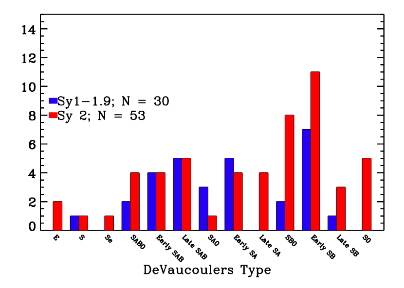
31 Sy1 and 54 Sy2 galaxies from the initial sample met all of these selection criteria, combined for a total of 85 Seyfert galaxies. This large sample ensures that the (Poisson) uncertainties from small number statistics are small. Our catalog includes significantly fewer Sy1 than Sy2 galaxies, partly due to a bias towards Sy2 AGN in the initial sample. For example, only 44% of the galaxies in MGT98 are classified as Sy1 AGN. In the Unified Model, this represents a bias in the opening angle through which the AGN is viewed. Though this bias may be present, it will not significantly affect this study, because we are investigating the core morphological distinctions between the AGN sub-classes of the host galaxies (i.e., on scales of hundreds of parsecs, well beyond the parsec scale of the thick, dusty torus). Where the data are available from NED, we plot the number of Seyfert galaxies by their deVaucouleurs galaxy type and 60m flux in Figures 1 & 2, respectively. These figures demonstrate that our catalog is not strongly dominated by a particular galaxy type or observed AGN luminosity.
We prepared the HLA mosaiced images for analysis by first visually identifying the (bright) center of each galaxy. We extracted a core region with physical dimensions of 22 kpc centered at this point. The HLA images that we used have only been processed to the Level 2 standard, i.e., only images acquired during the same visit are drizzled and mosaiced in the HLA. Many of the galaxies were originally imaged as part of HST snapshot surveys (single exposures with 500s). As a result, cosmic rays can be a significant source of image noise in the mosaics. We used the routine, (van Dokkum, 2001) to clean the CCD images of cosmic rays§§§available online at http//www.astro.yale.edu/dokkum/lacosmic/. Initially, we implemented using the author’s suggested parameters, but found by iteration that a lower value for the objectdetection contrast parameter, sigclip=2.5, produced cleaner images without significantly affecting the pixels of apparent scientific interest. Additional cleaning and preparation of the imaging was necessary for the following analyses, and we discuss those task–specific steps taken in §4.1.
3 Visual Classification of Core Morphology
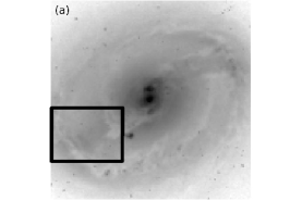
The core morphologies of the AGN–host galaxies are diverse and early– and late–type morphologies, with varying degrees of complexity in dust and gas features, are represented in the catalog. In Figure 1, we provide images of a subset (12) of our galaxies; each image has been scaled logarithmically. Images of all (85) galaxies are available in the electronic supplement to this article. Here, we use this subset of galaxies specifically to discuss the various dust features and structures that we classify by eye.
Galaxies in our catalog display a wide variety of spiral arms–like features. In Figure 1, we provide images of two galaxies (MARK1330, NGC3081) that show distinct spiral arms. These features are easily distinguished from the ambient stellar light profile in the core of each image. In some galaxies, these arms are reminiscent of galactic–scale spiral features, such as barred spirals (NGC3081). Some spiral–arm like features are more unique. For example, MARK1330 has a single arm that appears to in-spiral and connect with the bright core of the galaxy. Furthermore, some galaxies appear to be relatively dusty with numerous features of various size scales, appearing in either organized or chaotic features (e.g. NGC1068, NGC1386, NGC1672, NGC3393).
In Figure 1, we also provide examples of galaxies whose cores are relatively sparsely populated with dust features. In some cases (e.g., NGC3608), these galaxies have few dust features. In other galaxies (e.g., NGC1058) dust features appear most pronounced in the core of the galaxy (100-200 pc) and are less significant at large radii.
We have visually inspected and classified each of the 85 galaxies in our catalog, first using the following criteria that were defined and used in MGT98. We divide these criteria into two general classes
Class 1—Dust Classifiers
-
•
DI Irregular dust;
-
•
DC Dust–disk/Dust–lane passing close or through center (i.e., bi–sected nucleus);
-
•
D Direction of dust lanes on one side of major axis, where direction is N, S, E, W, NW, NE, SW, or SE;
-
•
F/W Filaments/wisps, and;
Class 2—Ancillary Classifiers
-
•
R Ring;
-
•
E/S0 Elliptical or Lenticular;
-
•
B Bar;
-
•
CL Cluster, lumpy H ii region, knots;
Four observers (PRH,HK,MJR,KT) inspected the 22 kpc postage stamp images in Figure 1 and classified each of the Seyfert cores. We did not use the “normal” classifier, because its definition could not be independently inferred from MGT98. In practice, we note that galaxies that showed regular spiral and dust features in their core morphology were more often classified as F/W. Conversely those with more irregular spiral and dust features was classified as DI. These classifications are not mutually exclusive, i.e., galaxies could be classified as both DI and F/W. In Table LABEL:tab:gallist all unique visual inspections are provided.
The majority (91%) of galaxies were identified with dust features. Irregular dust features (DI) were observed in 42% (13/31) of Sy1 and 57% (31/54) of Sy2 AGN. In contrast, 68% (21/31) of Sy1, and (31/54) 57% of Sy2 host galaxies, showed regular filaments and wispy features (F/W). Thus, by visual inspection, we find that Sy1 host galaxies are more regular in their dust morphologies than are Sy2 host galaxies, while Sy2 host galaxies are more chaotic or irregular in their dust morphologies than are Sy1 host galaxies.
To reduce ambiguity in the classification of regular and irregular dust features in our galaxies, and to provide a second confirmation of the MGT98 relationship, we developed an additional system specifically for the classification of the core dust morphology of Seyfert galaxies. This classification scheme is defined as follows
-
•
1-“Nuclear spiral”—Distribution of features resembles a flocculent or grand-design spiral;
-
•
2-“Bar”—A bar–like feature in emission or absorption extends outward from the center of the galaxy;
-
•
3-“Dust-specific classification”—The previous designations considered all structure. The following classifications describe only the quality and spatial distribution of what we consider to be dust
-
–
Group A
-
–
s-“Late-type Spiral”—Dust appears distributed in a spiral pattern throughout more than 50% of the image. The “inner-arm” regions appear to be clear of any dust;
-
–
i-“Irregular”—No visually distinguishable pattern can be identified in the spatial distribution of dust, i.e., the dust is patchy and irregular in form;
-
–
-
–
Group B
-
–
m-“High Extinction”—Dust features appear to be of high column density. The galaxy appears highly extincted. Dust lanes appear to “cut” through the ambient stellar light of the galaxy;
-
–
l-“Low Extinction”—Low contrast dust is present, but is barely discernible from the ambient stellar light.
-
–
-
–
In Table LABEL:tab:fitpars, we provide the classification using this scheme. If possible, galaxies were classified using Class 1 and 2, but all galaxies were classified according to their dust structure (Class 3). The sub-groups of Class 3 (A&B) were mutually exclusive; e.g., no galaxy could be classified as ‘3is’. Galaxies could be classified by a single Group A and one Group B classification simultaneously (e.g., ‘3mi’). If there was a conflict in classifying dust structure amongst the four co-authors, the majority classification is listed in Table LABEL:tab:fitpars. If no majority was reached after first classification, the corresponding author made the final classification without knowledge of the Seyfert class in order to prevent any unintentional bias in the measurement of the Malkan relationship.
The WFPC2 F606W filter we used in this image classification is broad (4800-7200Å) and includes the H[NII] line complex. In principle, this line emission could affect our visual classification. In practice, the contribution of line flux to the continuum is relatively minor — the contribution of the [NII] doublet to the total flux in this bandpass using the SDSS QSO composite spectrum (vanden Berk et al., 2001) is 1%, and we estimate the ratio of the equivalent widths, EW/EW[NII], of these lines to be . Despite the minor contribution to the total observed flux in line emission, the photo–ionization of the gas-rich local medium by the central engine can produce significant “hotspots” at the wavelengths of these atomic lines, which appear as structure in the image. Cooke et al. (2000) has studied an example of this photo–ionization structure, the spiral-like “S” structure in one of our sample Seyferts hosts (NGC3393; see Figure 1). Though this emission contributes very little to the total flux in the core, the high contrast between these bright emitting sources and the local area could lead to “false positive” classifications of dust features. Fortunately, few AGN (7-8 galaxies, see e.g., MARK3, MARK1066, NGC1068, NGC3393, NGC4939, & NGC7682 in Figure 1 of the online supplement) show evidence of these emitting structures and these highly localized structures are easy to distinguish, in practice, from the stellar and dust continuum.
In conclusion, we confirm that Sy2 host galaxies are significantly more likely to have irregular core morphologies 58% of Sy2 host galaxies were classified as ‘3i’. In contrast, only 40% of Sy1 host galaxies were classified as ‘3i’. Furthermore, 39% Sy2 AGN were classified as ‘3s’ in contrast to 53% of Sy1 host galaxies. The results of our visual classification agrees with the observations in MGT98.
Although visual inspection can be an effective means of classifying the morphology of spatially resolved sub–structure in galaxies, it has its disadvantages as well. Visual inspection is time–consuming, it does not provide a quantifiable and independently reproducible measure of the irregularity of structures that can be directly compared with the results of similar studies, and it can be highly subjective. Though guidance was provided to the co-authors on how to classify varying degrees of dust structure using the Class 3, such classifications are highly subjective and conflicts in classification could arise between co-authors. For example, approximately 55% of the visual classifications of dust structure (Table LABEL:tab:fitpars) were not unanimous. This discrepancy can be largely attributed to the subjective definition of the Class 3 sub-classifications. In each galaxy, the co-authors implicitly emphasized certain dust features when making their classification. In many galaxies, whether the authors chose to weight the significance of physically small or large-scale dust structure could change the structural classification significantly. Consider the case of NGC1365 this galaxy was classified with an irregular dust morphology due to the small-scale dust features that appear to dominate the visible sub-structure in the core. But, authors who (subconsciously or otherwise) emphasized the broad dust “lanes” in the north and (to a lesser extent) south may classify the core as having a “spiral” dust morphology. Neither classification is necessarily incorrect — the broad dust lanes are clearly associated with the prominent spiral arms in this galaxy when viewed in full scale. These complicating factors can weaken any conclusion drawn from the visual classification of galaxies.
In recent decades, as image analysis software and parametric classification techniques have become prevalent, the astrophysical community has implemented automated methods for galaxy classification (e.g., Odewahn et al., 1996; Conselice, 2003; Lotz et al., 2004). By relegating the task of object classification to automated software and algorithmic batch processing, these methods have gained popularity, because they can significantly reduce the time observers must spend inspecting each galaxy, and can provide a reproducible classification for each galaxy (cf. Lisker et al., 2008).
Therefore, we extend our original test of the Unified Model to include a quantitative assessment of the morphological differences between Seyfert galaxies that we identified by visual inspection. We present these techniques in §4 and §5. Our use of quantitative parameters to measure morphological distinctions between Seyfert core morphologies can provide a more robust test of the MGT98 relationship by reducing some of the biases implicit in visual inspection.
4 Traditional Quantitative Morphological Parameters
A variety of parameters have been defined in the literature to quantify galaxy morphology. These parameters are distinguished by their use of a pre-defined functional form—i.e., parametric or non-parametric—to express galaxy morphology. Some popular non-parametric morphological parameters are “CAS” (Conselice, 2003, “Concentration”, “Asymmetry”, and “clumpinesS”) and “Gini–M20” (Abraham et al., 2003; Lotz et al., 2004, “Gini Coefficient” and M20, the second–order moment of brightest 20% of the galaxy pixels). These methods are not without limitations (cf. Lisker et al., 2008), but they each can be useful for assessing galaxy morphology in a user–independent and quantitative way. We chose to use these parameters in this research project, because the distribution of dust features in the cores of Seyfert galaxies is unlikely to be well-described by a single functional form, e.g., the Sérsic function that broadly distinguishes between elliptical and spiral galaxy light profiles.
Conselice et al. (2000) provide the following functional definitions of the CAS parameters.
The concentration index, C, is defined as
| (1) |
where r80 and r20 are the values of the circular radii enclosing 80% and 20% of the total flux. The typical range in concentration index values measured for galaxies on the Hubble sequence is C (Conselice, 2004; Hernández-Toledo et al., 2008). Larger values of the concentration parameter are measured for galaxies that are more centrally peaked in their light profiles.
The asymmetry, A, is defined as
| (2) |
where x and y correspond to the length (in pixels) of the image axes, is the original image intensity, and is intensity of pixels in an image that is the original image rotated through an angle of (we set ∘). Typically, A ranges from 0 (radially symmetric) to 1 (asymmetric), see e.g., Conselice (2003).
Clumpiness, S, is defined as
| (3) |
where is the image intensity in pixel (a,b), is the pixel intensity in the image convolved with a filter of Gaussian width , and B(a,b) is the estimated sky–background for a given pixel. Typically, 0 S 1 (see e.g., Conselice, 2003), and galaxies that appear to be visually “clumpier” have higher values of S.
Abraham et al. (2003) and Lotz et al. (2004) provide the following functional definitions of the Gini–M20 parameters. The Gini parameter is defined as
| (4) |
where f̄ is the mean over all pixel flux values fj, and n is the number of pixels. This parameter measures inequality in a population using the ratio of the area between the Lorentz curve, defined as
| (5) |
and the area under the curve of uniform equality ( of the total area). Although this parameter was originally developed by economists to study wealth distribution, this parameter can be applied to understand the distribution of light in galaxies. If the distribution of light in galaxies is sequestered in relatively few bright pixels, the Gini coefficient approximately equals unity. The Gini coefficient is approximately equal to zero in galaxies in which the flux associated with each pixel is nearly equal amongst all pixels. In other words, the Gini coefficient quantifies how sharply peaked, or “deltafunction”like the flux in galaxies is. Note that this parameter can be affected by the “sky” surface brightness estimate assumed by the user, which we discuss in Appendix C.
The M parameter is calculated with respect to the total second–order moment, M, flux per pixel, , which is defined as
| (6) |
such that
| (7) |
where Mj is the second–order moment at a pixel , and (,) are the coordinates of the central pixel. In general, M20 typically ranges between M20 0 (Lotz et al., 2004, 2008; Holwerda et al., 2011). If considered jointly with the Gini coefficient, Lotz et al. (2004) determined that larger values of M20 (with correspondingly smaller values of G) are associated with “multiple ULIRG” galaxies, and that M20 is a better discriminant of merger signatures in galaxies.
We measure these five parameters—CAS and Gini–M20—to quantify distinctions between the distribution of light, which underpins the classifications we first made in (§3).
4.1 Case–specific Implementation of Traditional Morphological Parameters
The authors of CAS and G–M20 (Conselice, 2003; Abraham et al., 2003; Lotz et al., 2004, respectively) each defined a method to prepare images for analysis that accounts for systematic issues (e.g., compensating for bright or saturated cores of the galaxies). This method of image preparation and analysis also ensures that the parameters are measured for the galaxy itself, and that the contributions from background emission are minimized. In our analysis, we calculate all morphological parameters applying a functional form that is consistent with—or identical to—the form presented in the literature. However, we caution that our images and specific science goals require us to use an algorithm for image preparation and parameter measurement that differs slightly from the published methods. In this section, we outline key differences between our data and methods we used and those presented in the literature.
First, we measured these traditional parameters in images of galaxies observed at fundamentally different spatial resolutions (see §4.2). All galaxies in our catalog have been observed with HST WFPC2 at a pixel scale of 010 pix-1. In contrast, CAS and Gini-M20 are often measured from images obtained with ground–based telescopes that have relatively low spatial resolution in comparison with HST. For example, Frei et al. (1996) present images obtained with the Lowell 1.1 and Palomar 1.5 meter telescopes at 20 resolution at full–width half maximum (FWHM). This data set has been used extensively to test the CAS and Gini-M20 parameters’ ability to discriminate between the morphological classes and star–formation histories of nearby galaxies (e.g., Conselice, 2003; Lotz et al., 2004; Hernández-Toledo et al., 2006, 2008). The vastly different spatial resolutions between images obtained at ground–based observatories and the HST images implies that the parameters that we measure are sensitive to features of fundamentally different sizescales. In fact, in ground-based images most of the small–scale structure that we identified and used to classify the galaxies (§3) is undetected. Thus, parameters that are dependent on the pixel–specific flux values (e.g., M20), rather than on the average light distribution (e.g., concentration index), may be more sensitive to these spatialresolution differences because at lower resolution fine–scale structure are effectively smoothed out. In Appendix A, we quantify the effect of spatial resolution on the specific criteria that we use to characterize the structure of dust features in our Seyfert galaxies.
In Conselice (2003) and Lotz et al. (2004), the CAS and Gini-M20 parameters, respectively, are all measured in an image that is truncated at the Petrosian radius of the galaxy. The Petrosian radius is defined as the radius () at which the ratio of the surface brightness at to the mean surface brightness of the galaxy interior to equals to a fixed value, , typically equal to 0.2. A Petrosian radius or similar physical constraint is applied to differentiate between galaxy and sky pixels, and ensures that the influence of background emission is minimized in the calculation of CAS and G-M20. The mean Petrosian radius measured in the r′ –filter (=6166Å) of Sloan Digital Sky Survey (SDSS) Data Release 7 is 4.3 kpc¶¶¶Only 28 galaxies in our catalog were observed in SDSS DR7, available online at http://www.sdss.org/dr7, but those galaxies common to our survey and SDSS span a range of morphologies and distances, hence we consider the measured mean Petrosian radius to be representative for our catalog.. Since we are not interested in the contribution of dust features located at radii greater than 1 kpc, we do not use images truncated at rp. Furthermore, at the mean redshift of our sample, the WFPC2 PC chip field of view is 2.8 kpc.
Unlike observations of the entire galaxy, in our core images we can make the reasonable assumption that most of the flux that we observe in the core arises from sources or features physically associated with the galaxy. Not all pixels are sensitive to the flux arising from the galaxy, though, and we use the following method to differentiate between the light arising from galaxy sources and other extraneous objects or noise.
-
•
We set all pixels that occur at the edges and the chip gaps between the WFC and PC CCDs in the mosaiced images equal to zero. Furthermore, the center of the galaxy is often much (10–100) brighter than the rest of the galaxy, likely due to the AGN emission. To avoid such extremely bright pixels from biasing the measurement of any of the automated classification parameters, we set a high threshold defined as the average of the inner–most 55 pixels for each galaxy. We set the pixel values above this threshold equal to zero in the CAS & G–M20 computations.
-
•
If the functional form of a parameter explicitly required a background term, we set this term equal to zero. Our analysis is focused on the cores of each galaxy (1 kpc; or less than 0.5), which are significantly brighter, and have high enough surface brightness, that the contribution of background objects can be considered to be minimal. We assume that our images include only light from the galaxy itself and background emission from the zodiacal (foreground) light, which arises from sunlight scattered off of 100m dust grains. Fortunately, from the generally dark HST on-orbit sky, the actual zodiacal sky surface brightness is a simple well–known function of ecliptic latitude and longitude (). We use measurements of the zodiacal background from WFPC2 archival images presented by Windhorst et al. (in prep.), to estimate the emission from this dust in the F606W band. The average on–board HST F606W–band zodiacal sky brightness can be found in Table 6.3 of the WFCP2 Handbook McMaster et al. (2008), but the values in Figure 2 give a more accurate mapping as a function of & . The zodiacal background could not be directly calculated from the images, because the galaxy core typically over–filled the CCD. We correct for the zodiacal foreground emission prior to image analysis in §4.2 and §5.1. For more details, see Appendix C.
-
•
To measure clumpiness, we included an additional processing step motivated by the algorithm defined in Hambleton et al. (2011). Prior to calculating the clumpiness parameter as defined in Conselice (2003), we first applied a 55 pixel boxcar smoothing to the input image. We produced the residual map by subtracting the smoothed galaxy image from the original input image. The additional smoothed image was generated by applying a boxcar smoothing kernel with the one–dimensional size of kernel defined as , where is the dimension of the galaxy image in pixels. By design (see §2), the linear size of the smoothing kernel is equivalent to or 0.67 kpc. If we assume that 4 kpc is approximately equal to the Petrosian radius for each galaxy in the sample, then this dimension is comparable to the smoothing kernel size applied in Conselice (2003) and Hambleton et al. (2011). We tested this assumption of an average Petrosian radius, and found that using a larger or smaller value (kpc) for the linear dimension of the kernel has less than 1% effect on the measurement of clumpiness. In this analysis, we also set all pixels within 10 of the galaxy center equal to zero.
In the subsequent analysis, we removed all zero–valued pixels to prevent those pixels from affecting the calculation of any of the parameters.
Though we use identical—or nearly identical—functional definitions of each morphological parameter used in the literature, we are analyzing regions of our galaxies at size–scales that are significantly different than have been used in previous research. As a result, we cannot assume that our parameter measurements are directly comparable to the CAS and GM20 traditional measurements in the literature (e.g., Conselice, 2003; Lotz et al., 2004). We therefore refer to our parameters that we derived using the above criteria hereafter as and –, in order to distinguish our measurements from the traditional parameters presented in the literature.
4.2 Analytical Results and Discussion
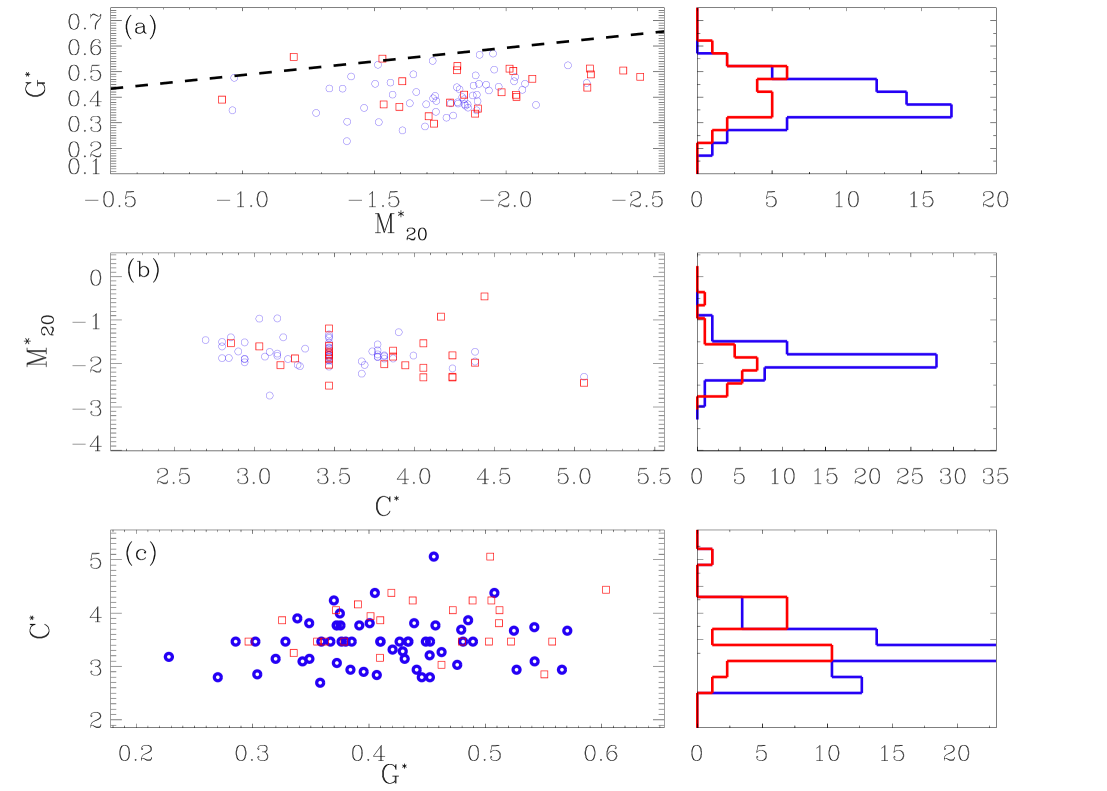
Figure 3 provides three permutations of the measured –– parameters. In this figure, Sy1 and Sy2 host galaxies are represented in blue and red, respectively. We use this color scheme for all figures provided in the online version of this manuscript to distinguish our measurements for the two classes of Seyfert galaxies. It is noteworthy that the distribution of each of these parameters spans a range that is comparable to the range of the G, M20, and C measured from ground-based images at the lower spatial resolution (0.7 0.1, 2.5 , 2.5 5.5).
In Figure 3(a) we overplot a dashed line that differentiates “normal” galaxies (which reside below this line) from starburst galaxies or ULIRGs (i.e., Ultra Luminous Infrared Galaxies) as defined in Lotz et al. (2004). Four of our Seyfert galaxies are measured to be on or above this line NGC1672, NGC4303, NGC4395, NGC7469. The fact that these galaxies reside in this parameter space is appropriate, since these four galaxies are considered to be starburst or circum-nuclear starburst galaxies in the literature. However, approximately 32% of the Seyfert galaxies were identified in the literature as starburst or circum–nuclear starburst galaxies. Hence, we conclude that and do not effectively discriminate between “normal” and starburst galaxies, as these parameters are demonstrated to do in the literature. We note that - are used to distinguish starburst and “normal” galaxies when the complete galaxy morphology is considered. The morphology of the galaxy on this scale need not necessarily match with the core morphology of the galaxies.
We can consider the relative distribution of the – values measured for our AGN. In Figure 3(a), we fit a Gaussian function to the and distribution and measure the shape, centroid, and peak of this function for both Sy1 and Sy2 AGN to be comparable. The parameters of the fitted Gaussian function are provided in Table LABEL:tab:spartab1.
We can draw similar conclusions as above from the distribution of and presented in Figure 3(b) and (c), respectively. First, it is noteworthy that is well–distributed in the same parameter space spanned by the conventional concentration index, when it was calculated for the entire galaxy at lower spatial resolution. We fit a Gaussian to the distribution measured for Sy1 and Sy2 AGN, and measured comparable values for the centroid and FWHM of each distribution (see Table LABEL:tab:spartab1).
We perform a two–sample Kolmogorov–Smirnov (K–S) for the Sy1 and Sy2 distributions to test whether these distributions are self–similar. The two–sample K–S test can be used to measure the likelihood that two empirical distributions were drawn as independent samples from the same parent distribution. We use the K–S test here for two reasons, in contrast to more commonly measured statistical parameters (e.g., the statistic) 1) the sample size for each distribution is small, which can lead to an incomplete distribution; and 2) a priori we do not know the parent distributions from which the empirical distributions were drawn. We use the IDL routine kstwo to measure the K–S statistic, d, which equals to the supremum distance between the cumulative distribution functions (CDF) of the input distributions. kstwo also reports the probability statistic, p, which is the likelihood of measuring the same supremum in a random re-sampling of the parent distributions expressed by the empirical distributions. The K–S test cannot provide any insight into the parent distribution(s) from which the empirical distributions are drawn, but it can be used to test the null hypothesis that the empirical distributions were drawn from the same parent distribution. When the K–S statistic is small or the probability is large (p0.05), the null hypothesis cannot be rejected with confidence.
The results of the K–S test for the and parameter distributions are provided in Table LABEL:tab:spartab1. These distributions are indistinguishable for both Seyfert classes. However the K–S test measures a slightly larger values of d=0.38 for the distribution of C∗, indicating that the CDFs are distinct. The associated probability statistic for is small (p=0.01). We conclude that the distributions measured for Sy1 and Sy2 are significantly different, and thus are likely to be drawn from unique independent parent distributions. This could support the morphological distinction between the cores of Sy1 and Sy2 galaxies that was identified by visual inspection in §3. In contrast, if – are indeed sufficiently robust metrics for distinguishing the distribution of light in the cores of these Seyfert galaxies, then the results of the K–S test suggest that these parameters do not quantitatively distinguish the galaxy morphologies of Sy1 and Sy2 AGN.
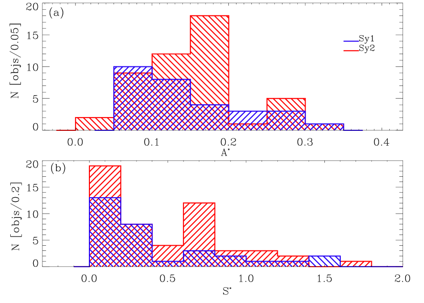
We consider the (asymmetry) and (clumpiness) parameters independently from the – parameters, because we believe that these parameters are best able to identify—by design—the dust features that we found by visual inspection. In Figure 4(a), we present the distribution of measured for our AGN. We did not calculate asymmetry for NGC1058, NGC1386, NGC1672, NGC3486, NGC4051, NGC4303, NGC4395, and NGC4698, because the WFPC2 images of these galaxies included off–chip regions that were set to zero (see §4.1). These regions can seriously affect our measurements because asymmetry is calculated by differencing a rotated image with the original. In Figure 4(b), we present the distribution of &. We fit Gaussian functions to the distributions of and measured for Sy1 and Sy2, respectively. The best–fit Gaussian function to each distribution are provided in Table LABEL:tab:spartab1. The Gaussians’ parameters measured for Sy1 and Sy2 galaxies appear to be indistinguishable. We confirm this via a two-sample K–S test for the and distributions. The results of this test are presented in Table LABEL:tab:spartab1. We conclude from this test that both parameters distributions are likely drawn from the same parent distribution.
The uniformity in the & G∗-M distributions also suggests that the H[NII] emission arising from the photo–ionization of gas (see §3) does not strongly affect the measurement of these parameters. Furthermore, if the and parameters are suitable metrics for quantifying the morphology of galaxies, then the results of this quantitative analysis do not support the correlation between core dust morphology and Seyfert class established by MGT98 and confirmed by our visual inspection in §3.
In conclusion, four of the five quantitative parameters ( and ) measured for the galaxies do not support the qualitative conclusions developed from visual inspection. The distribution of may be specific to the class of AGN, which could support the MGT98 relationship, but this parameter is the least–suited, by design, to quantify the morphological distinctions that supported the morphology–AGN class correlation. We note that this does imply that the MGT98 relationship is invalid, but that the use of the & – parameters to confirm this distinction may not be optimal.
5 Quantitative Morphology with Source Extractor
The results of the previous analysis may imply that & – parameters are insufficient as tools to distinguish the sub–kiloparsec scale features in AGN. In this section, we therefore develop an additional non–parametric technique that uses Source Extractor (Bertin & Arnouts, 1996, hereafter, SExtractor) to measure the distribution of dust features in the cores of AGN host galaxies.
SExtractor is an automated object detection software package that generates photometric object catalogs. This software is widely used for photometry and star/galaxy separation in UV–optical–IR images partly due to the software’s speed when applied to large image mosaics. A review of the literature returns more than 3000 citations to Bertin & Arnouts (1996), with applications extending even beyond astrophysics (e.g., medical imaging of tissue cultures by Tamura et al., 2010). The versatility of SExtractor to detect and measure the properties (e.g., aperture photometry) of galaxies motivated us to adapt SExtractor for our purposes. In our study, we use SExtractor only for object detection, because the algorithm we outline (§5.1) and apply (§5.2) may prevent accurate photometry.
SExtractor has often been used in the study of nearby, dusty galaxies (see recent work by Kacprzak et al., 2012; Holwerda et al., 2012, for example). This research does not employ SExtractor to directly detect and measure the properties of the absorbers. Rather, SExtractor is used to derive the photometric properties of galaxies, and these data are coupled with the dust properties of the galaxy (e.g., covering fraction). In §5.1, we adapt SExtractor to directly detect dust features that are visible to the eye. Thus, our use of SExtractor to outline the characteristics of dust features that are fundamentally seen in absorption is a unique application of this software.
5.1 Technical Implementation to Identify Dust Features
In this Section, we outline the method we used to train SExtractor to identify “objects” that we visually identified as dust features, effectively using this software to mimic the human eye.
To detect these objects, SExtractor first calculates a local background, and determines whether the flux in each pixel is above a user–defined threshold detect_thresh. All pixels exceeding this threshold are grouped with contiguous pixels that also exceed this threshold. When a sufficient number (defined by the detect_minarea parameter) of contiguous pixels are found to meet the signal threshhold, the pixel group is recorded as an object in the object catalog. Finally, SExtractor measures a variety of parameters (e.g., object center, total flux, size, orientation), and constructs a segmentation map of detected objects.
To detect objects corresponding to the visually detected dust features in the cores of our galaxies, it was necessary to first train SExtractor using the WFPC2 images of the Seyfert host galaxies. Initially, we used the HLA image of each galaxy—appropriately cleaned of defects as detailed in §2—for object detection. After extensive testing, we could not determine a suitable combination of the parameters detect_minarea and detect_thresh that would force SExtractor to identify a set of comparable objects to the set of dust features that we visually identified in §3. By setting detect_thresh low enough that nearly all visually identified dust features are recovered, too many of these features were broken into multiple unique objects. To alleviate the over–segmentation, we increased the detect_minarea parameter. In order to recover the majority of the visually identified dust features though, this parameter must be set unfavorably high; dust features were only detected when they were included as a component of a much larger, brighter object.
Direct detection of dust features with SExtractor is difficult. This can be directly attributed to the manner in which SExtractor detects objects. SExtractor is designed to detect peaks above the local background. In the images, the local background is bright, and not likely to be smooth because it arises from the ambient stellar background and not the astronomical/zodiacal sky. Furthermore, SExtractor can not detect many of the dust features as they are observed in absorption with respect to the background. These absorption features may be brighter than the true astrophysical background, but they are still fainter than the local background. Thus, no optimal SExtractor parameters can be defined to exclusively select the visually identified dust features.
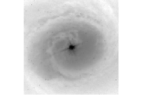
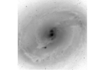
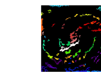
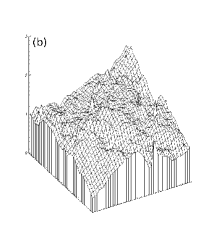
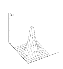
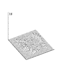
We therefore trained SExtractor to identify objects that more closely matched with dust features identified (§3) by coupling object detection using SExtractor with the “unsharp–mask” technique. The unsharp–mask is a common tool for image analysis, because it enhances features of specific spatial scales. In astronomical images, these features correspond to physical objects, such as stars, star clusters, and/or dust clouds. To apply this procedure, we first convolved the WFPC2 images with a Gaussian convolution kernel to create a smoothed image. Next, we divided the convolved image by the original image to produce the inverse unsharp–mask image (hereafter, IUM)∥∥∥The unsharp–mask image is typically produced by either differencing or dividing the original image by the convolved image. When the contrast between the original and the convolved image is small, as it is in our WFPC2 images, these two different calculations yield similar results.. In principle, if we appropriately define our convolution kernel such that it enhances these structures of specific size–scales corresponding to dust features and apply the IUM, those features should now be detected as a positive signal above the local background using SExtractor with the appropriate detection parameters. In Figure 6, we provide an illustration of this technique. In Figure 6a&6b) we show the core image of NGC3081 and a surface map of an inter–arm region. We convolved the image with a kernel (Figure 6c), and apply the IUM technique to produce Figure 6d. In this figure, it is apparent that the dust features in the region of interest have been enhanced by the IUM technique.
To produce the IUM image of each galaxy, we first assumed that giant molecular clouds (GMCs) are physically associated with dust features. We generated a Gaussian convolution kernel that is specific to each galaxy, the properties of which were motivated by observations of GMCs. To produce the appropriate convolution kernel, we first used the galaxy’s redshift from NED to define a physical pixel scale (; pixel kpc-1) of the kernel. The linear size scale of GMCs is typically less than 100 pc (see Casoli, Combes, & Gerin, 1984; Fukui & Kawamura, 2010), so we defined the FWHM of the kernel equal to /, initially with =100 pc. We tested a range of size scales, and determined that =80 pc optimally enhanced the sub–kiloparsec scale dust features that we visually identified in §3. We also determined the appropriate linear size of the kernel to be equal to x/10, where x is the length on each axis of the image in pixels.
We determined optimal SExtractor parameters by an iterative process to find the segmentation map that most faithfully reproduced the dust features classified in §3. In this process, we fixed the SExtractor parameter detect_minarea equal to 90.0/ for all objects. We required detect_thresh for each object pixel to be at least 1.5 above the local sky–background in the IUM image. Additionally, we determined that the default values for the SExtractor parameters deblend_nthresh and deblend_mincont equal to 32, and 0.03, respectively, were sufficient for dust feature detection in the IUM image.
We discuss the results of implementing our method using the optimized parameters in §5.2. The algorithm we have outlined above for the detection of dust features in absorption in images is generic. It is not applicable exclusively to our specific scientific interests. Thus, we prepared all IDL procedures that we developed to implement this technique for the public. Readers who wish to apply this method to other science topics are encouraged to email the corresponding author.
5.2 Results and Discussion
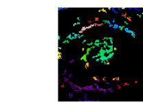
In Figure 1, we presented a four–panel mosaic of 12 galaxies including the WFPC2 galaxy core image and its corresponding SExtractor segmentation map. The first of these images was discussed in §3. To produce the second image, we reproduced the segmentation images in DS9 using the built–in “SLS” color map******more details are available online at http//hea-www.harvard.edu/RD/ds9/. This 256–bit “rainbow” color map including black and white allows our eyes to better distinguish between different detected objects. However, when the total number of detected objects () is greater than 40 even this color map is insufficient to distinguish between all unique neighboring sources. As a result, many unique objects may appear at roughly the same color, although these are not necessarily detected as the same object. This limitation of the color map does not affect our calculation of . Furthermore, for most galaxies the segmentation maps show a number of objects near the edge of the image. Although some of these edge detections may be related to real dust features, we excluded these edge detections in the subsequent analysis and discussion.
A comparison of the segmentation map and the galaxy core images suggests that our general SExtractor technique is remarkably successful in recovering only those dust features that we identified first by visual inspection. Specifically, the dust feature recovery rate using the IUM technique is very good for the majority (95%) of the catalog. For example, bar and spiral arm–like features are well-recovered as unique objects (see, e.g., MARK1330). The fidelity of the object detection of the spiral arm features is often high enough in these galaxies (see,e .g., NGC3081) that the spiral arm features in the image are entirely reproduced in the corresponding segmentation map.
Galaxies with relatively many dust features—in both regular or chaotic spatial distributions—also appear to be faithfully reproduced in their associated segmentation maps. For example, the regular structures in NGC1068 and NGC1066 are detected with SExtractor as are the more chaotic dust features, as seen in ES0137–634 and ESO323–G77. An interesting result of this IUM analysis is that the objects in some galaxies (e.g., NGC1386, NGC1672) are sometimes limited to particular quadrants of what appears to be a disk in the original image. The distribution of dust features suggests to the eye that this disk (in which the features are embedded) is moderately inclined towards the viewer. A discussion of molecular toroid inclination effects are beyond the scope of this work, but we will consider this result in future work. We note here that this disk inclination was identified first and only by using the SExtractor technique.
In images where the stellar light profile is exceptionally smooth and few dust features are identified by visual inspection, the IUM technique may detect objects that do not strongly correlate with the dust features visually identified in §3. This may represent a limitation of our IUM technique. In Figure 1, we included the images of two galaxies (NGC1058 and NGC3608)††††††Only four galaxies—MARK348, MARK352, NGC1058, NGC3608—showed any strong distinction between the number, size, and spatial distribution of objects detected with SExtractor segmentation map and dust features noted by visual inspection in §3. that represent this small fraction () of the catalog galaxies. We do not remove these galaxies from the subsequent analysis for completeness and to illustrate to the reader instances when our SExtractor technique may be limited in its ability to discern visually identified dust features. We caution that object detection in these few galaxies using our IUM technique may be more sensitive to local pixel–to–pixel noise variations than it is to signal variations arising from dust absorption.
Furthermore, in those galaxies that appear to have photo–ionization structures (see §3), the number and distribution of dust features using the IUM technique still appears to be very well-correlated with the visually-identified dust features (see, e.g., NGC3393 in Figure 1). In some galaxies, the potential photo–ionization structure appears to be the brightest structure visible in the image. It does not appear that this high contrast between photo–ionization structures and the visually-identified galactic dust structure has strongly affected the dust feature detection using the IUM technique. Variations in the mean signal across these structures could affect the calculation of the local sky background with SExtractor, and thus influence dust feature detection in those galaxies with possible photo-ionization emission structures. For example, such variations could explain the segmentation of what appears as one chaotic dusty region into two approximately equal area dust features along the outer edge of the northeastern “spiral-arm” photo-ionization structure in NGC3393.
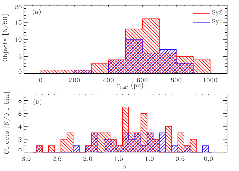
We also provided in Figure 1 two measurements of the characteristics of the dust structure quantified with the IUM technique. We plot the cumulative number of objects for each galaxy contained within circular annuli centered at each galaxy’s core for a radius , where and =2.0 pixels. Although we present square images of the galaxy, we only calculate the cumulative number for annuli with radii less than 1 kpc in the frame to remove edge detections. Using the cumulative object number distribution, we calculate a half–object radius () defined as the radius (in pixels units) of the annulus that contains the inner 50% of the total number of detected objects in each galaxy. This value is provided in physical units (parsecs) with measurement uncertainties in Table LABEL:tab:fitpars.
In Figure 6(a) we plot the distributions of . We fit a Gaussian function to the distribution of for Sy1 and Sy2 galaxies and provide the parameters of the best–fit functions in Table LABEL:tab:spartab2. There is no apparent distinction in the distribution of half–object radii between Sy1 and Sy2 galaxies. This is confirmed by a two–sample K–S test, the results of which indicate that the parent distributions from which the half–object radii distribution were drawn are not likely to be unique.
Figure 1 also included the object surface density distribution () measured for the galaxies, which we defined as
| (8) |
where N is the number of objects contained within annuli of width equal to 10 pixels. We fit a linear function to the object surface density function versus radius and measure the best–fit slope (). In Figure 6b, we provide the distribution of measured. We fit a Gaussian function to the distribution of as measured for the two classes of AGN, and measure the Gaussian centroids and FWHM to be nearly equal (Table LABEL:tab:spartab2). The similarity in the distributions is confirmed by a two-sample K–S test. Thus, the distribution of the object surface density functions does not appear to be unique to the class of AGN.
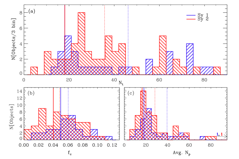
In Figure 7a, we plot the number of objects () identified in each galaxy. We measure the centroid and half–width half maximum (HWHM) of both the Sy1 and Sy2 distributions (see Table LABEL:tab:spartab2). We fit a Lorentzian function, rather than a Gaussian function, to better account for the broad extension from the HWHM peak to large object numbers in the distribution. The centroid of the best–fit Lorentzian function of objects equals to 18 for both classes of AGN, but the mean value of the Sy1 and Sy2 distributions equals to 47 and 35, respectively. Thus, these distributions appear to be significantly different. We confirm this result via a two–sample K–S test we measure d=0.35 and p=0.01, and conclude the empirical distributions of measured for the Sy1 and Sy2 populations are likely drawn from independent parent distributions. If the objects detected with SExtractor physically correspond to dust features in the galaxies, then we may conclude that Sy2 galaxies are, on average, dustier than Sy1 galaxies. If we remove the four galaxies discussed above for which our SExtractor technique did not appear to detect objects that are closely associated with the dust features that we identified by visual inspection, though, we measure the K–S test probability statistic for the distributions of equal to p=0.06. In this case, we can not reject the null hypothesis, and instead are forced to conclude that the distributions of measured for Sy1 and Sy2, respectively, were likely drawn from the same parent population.
The MGT98 relationship did not consider the number of dust features explicitly, but the assignment of relative degrees of dustiness to galaxies implicitly reflects the number of dust features that were identified visually. It seems to the authors that is easier to visually classify the dust structure as irregular if it contains a relatively large number of dust features, because the eye can more readily identify absorption patterns and divergences therefrom. Thus, the mean measured for Sy1 and Sy2 (Figure 7a) may support—albeit indirectly—the MGT98 relationship in a quantitative way.
In Figure 7b and 7c, we also provide the covering fraction () and the average number of pixels () associated with objects detected by SExtractor. We fit a Gaussian function to the distributions measured for each of these parameters, and observe no distinction between the Gaussian centroid or FWHM measured for Sy1 and Sy2, respectively (see Table LABEL:tab:spartab2). We confirm the similarity between the measured distributions by a K–S test, and conclude that these distributions are likely drawn from the same parent distribution. These results would not support the MGT98 relationship, or at least not demand it.
Throughout this work we have considered the results of our only in the context of the Unified Model, as outlined in Antonucci et al. (1993). We restricted our discussion of these results to this context, in part, because we were motivated in this work to extend the analysis first presented in Malkan, Gorjian and Tam (1998), in which the authors make a similar assumption on the nature of AGN. The assumption of this model is still fair; despite extensive debate (see §1) the Model provides a remarkably robust explanation for the observed diversity of AGN‡‡‡‡‡‡If only because many of the systematic considerations of the Unified Model are still, regrettably, limited by large measured uncertainties; cf. Guainazzi et al. 2011. But this model is not without rivals. For example, the “clumpy torus” model reduces the thick, dusty torus—the inclination of which gives rise to the observed dichotomy of Seyfert-type AGN—to distinct individual dust clumps that are generally distributed about the central engine. In this model, the AGN type that one observes is not a “binary” function of perspective; rather, the probability of observing a Type 1 AGN decreases as the viewer moves towards an “edge-on” perspective but never reaches zero. We observe a core region that is hundreds of parsecs beyond the toroid, though. Thus, a full interpretation of our results in the context of this model is beyond the scope of this project and we reserve that discussion for future work.
6 Conclusions and Summary
Recently, multi–wavelength high spatial–resolution images and spectroscopy of AGN–host galaxies have revealed that the characteristics (e.g., morphology, dust, properties of the emission line regions; see §1) of these galaxies may not be consistent with the Unified Model of AGN. In particular, HST WFPC2 imaging of the cores of local ( 0.035) Seyfert–host galaxies established that the morphologies of dust features in these galaxies correlates with the AGN class (MGT98). We investigated this trend by visually inspecting a catalog of archival WFPC2 F606W images of the cores of 85 local () Seyfert galaxies, and classified these AGN by the presence and distribution of dust features in each. We determined that Sy2 galaxies were more likely to be associated with galaxies whose core dust morphology is more irregular and of “later–type” morphology. Thus, our visual classification of our Seyfert galaxies confirms the qualitative morphological relationship established by MGT98. We concur with the conclusion of MGT98 that—if this morphological relationship is indicative of a fundamental distinction between the subclasses of AGN—this result weakens the central postulate of the Unified Model of AGN.
We extended the study of this morphological relationship established through the qualitative visual method by re– analyzing the images using quantitative morphological tools. First, in §4.1 and §4.2, we developed and measured the and – parameters for the galaxies. The distribution of these parameters as measured for Sy1 and Sy2 AGN did not strongly distinguish between the Seyfert class and morphology of the host galaxy. We determined that the parameter distributions for Sy1 and Sy2 AGN are likely drawn from the same parent distribution using a two–sample K–S test, with the exception of the concentration parameter. In comparison with the other four parameters in this set, though, is the least sensitive parameter to the morphological features identified and classified by visual inspection. We conclude from this analysis that no strong morphological distinction exist between the cores of the Sy1 and Sy2 AGN host galaxies. This conclusion conflicts with the established MGT98 relationship which we have visually confirmed in §3.
In order to resolve these apparently conflicting conclusions and to address the possibility that the and – are less effective tools for characterizing sub–kiloparsec scale dust features, we developed a new method to quantify the core dust morphologies of the AGN galaxies. This method combines SExtractor with the IUM technique. We applied this method and found that the distributions of the average number of detected dust features in Sy1 and Sy2 AGN may be different. Thus, we have measured a quantitative distinction between Sy1 and Sy2 AGN that supports the MGT98 relationship. Yet, there was no concordance between this result and any other result (i.e., the radial distribution, size and covering fraction of dust features) derived from this quantitative method. We therefore cannot strongly distinguish between Sy1 and Sy2 AGN on the basis of their core morphologies using this quantitative method.
In conclusion, we studied the relation between the host galaxy core ( kpc) morphology and the Seyfert class of AGN. We find evidence to support this conclusion from the results of a quantitative assessment of the core dust morphology using existing and new methods. However, we can not strongly distinguish between the core dust morphology of Sy1 and Sy2 AGN using the complete set of morphological parameters. Thus, we are reluctant to suggest that the Unified Model of AGN must be significantly modified to accommodate the results of this qualitative and quantitative analysis. In the future, better and more internally consistent qualitative and quantitative methods need to be developed to elucidate the true nature of the cores of Seyfert galaxies. We expect that JWST will be able to do a similar investigation of this topic at longer wavelengths, thereby penetrating deeper into the Seyfert galaxies central dust.
7 Acknowledgements
This work is supported by NASA ADAP grant NNX10AD77G (PI: Windhorst). The Hubble Space Telescope is operated by the STScI, which is operated by the Association of Universities for Research Inc., under NASA contract NAS 5–26555. We make extensive use of the HLA, the online repository of HST data that is maintained as a service for the community by the Space Telescope Science Institute, and SDSS Data Release 7. The authors acknowledge S. Kenyon, R. Jansen, S. Cohen, J. Bruursema, M. Benton and Y. K. Sheen for helpful technical support and scientific discussion. M. Rutkowski acknowledges the U.S. State Department Fulbright Program for financial support of this research.
Appendix A A. Spatial Resolution Ground vs. Space–based imaging
We implicitly assumed throughout this paper that HST images are necessary to conduct the quantitative morphological analyses. If lower spatial resolution ground–based optical images could be used instead of the high spatial resolution HST images, we could significantly increase the number of galaxies we can consider. The SDSS archive, for example, could provide images of hundreds of local AGN.
We downloaded SDSS r′ images for 7 AGN that were in both the SDSS DR7 archive and our catalog presented in §2. We made thumbnails of the core (1 kpc) SDSS images of each galaxies and measured and parameters using the same techniques outlined in §4.1 for each galaxy. In Figure 8, we compare these measurements with those presented in §4 which were measured in HST F606W images. It is apparent from this comparison that and cannot effectively discriminate between the morphologies of the SDSS galaxies. This result confirms that the quantitative morphological analysis we performed above requires the high spatial resolution HST images.
Appendix B B. Size–Scale Relation
Two galaxies that are identical in every possible way (e.g., morphologically), but at significantly different distances from an observer, will appear different in images obtained with the same telescope, because each CCD pixel covers an intrinsically larger physical area in the more distant galaxy. As a result, the dust features in the more distant galaxy are less well–resolved spatially. Our catalog includes galaxies in the range between 0.001 0.015, or equivalently a factor of 10–15 in physical distance.
We selected six galaxies—NGC1068, NGC3185, NGC3227, NGC3608, NGC4725, NGC4941—with morphologies that represented the diversity of morphologies in our catalog. These galaxies are all at distances 15 Mpc, and we use these galaxies to quantify the extent to which we are able to identify or measure dust features in our catalog galaxies as a function of distance. We do not use the nearest galaxies ( 10Mpc) in our catalog because these galaxies include large off–chip regions that significantly affect the measurement of asymmetry.
We then rebinned each of these galaxies to a pixel scale, s, such that
| (B1) |
where is number of WFPC2 010 pixels spanning 1000 pc at the physical distance, D, to the galaxy and corresponds to the distance to a galaxy at the upper redshift range of galaxies in our catalog (63 Mpc).
We measure and – for these artificially–redshifted galaxies and compare the measured values with the original measurements (§4.2). This comparison is presented in Table 5 as , where X and Y are the morphological parameters measured in galaxy images at and artificially redshifted to .
In general, the measurement of these parameters does not seem to be strongly affected by the relative distance of the galaxy, at least over the relatively small redshift range that we consider in this project. For all parameters, is much smaller than the measured dispersion in the range of parameters measured in §4.2. We conclude that range of measured parameters (see Figures 3 and 4) are indicative of morphological distinctions between the cores of the sample galaxies, as we assumed in the discussion in §4.2.
Appendix C C. Sensitivity of measurements to the estimated sky–background
Windhorst et al. (in prep.) measured the surface brightness of the zodiacal background as function of & from 6600 WFPC2 F606W and F814W Archival dark–time images. We reproduce these measurements for the F606W zodiacal background from Windhorst et al. (in prep.) in Figure 2. In §4.1 we estimated the surface brightness of the zodiacal background along the line–of–sight to each galaxy in our catalog. We made the reasonable assumption that the only background emission present in the images in the cores of our catalog galaxies arises from the zodiacal background and then corrected for this background alone in each image.
In this section, we measure the uncertainty in our measurements of and – and the object surface density distribution associated with our assumption of the brightness of the background in the images. In general, the brightness of the background is determined to have a minimal effect on these parameters, with the notable exception of , and to a lesser extent, the slope parameters. In Figure 10, we compare the measurements of for galaxies corrected for a zodiacal background equal to a) zero (); b) the Windhorst et al. background (); and c) a hypothetical background 10 times larger than the measured in Windhorst et al. The latter estimate of the background emission is highly unlikely in any HST image (see Figure 2). We assume such a large background here only to provide an upper extremum to our measurement of the effect of the background surface brightness assumption.
The dispersion measured for most parameters, i.e., and , for different estimates of the zodiacal surface brightness was small (1%). There is a large dispersion between and . We attribute this dispersion to the removal of relatively faint pixels from the measurement of as increasingly larger values for the sky surface brightnesses are subtracted from the images. This has the net effect of (artificially) enhancing the flux associated with relatively higher signal pixels, which increases .
We note that there is a modest increase in the measurement of (the slope of the object surface density function), when comparing cases (a) and (c). The net effect of background on this measurement is less than 5%. Hence, blindly adopting the most likely zodiacal sky–brightness as a function of & —when this background is not directly measurable—is an acceptable and, in our case the only viable, approach.
Appendix D D. IUM Technique Dust Feature Detection Threshold
The detection of dust features with Source Extractor is explicitly dependent on the detection parameters defined by the user in the configuration file. Here we discuss the typical contrast level of the dust features, relative to the “sky background” in the images, which SExtractor detected for those parameters outlined in §5.1. We define the “contrast” as:
| (D1) |
where is the flux associated with a detected object using the IUM technique and is the average sky value measured in a uniform “sky” region drawn from the core image.
We measured the contrast parameters for two representative galaxies in the sample, NGC3081 and NGC3608. The IUM technique appears to work very well in detecting the dust clumps in NGC3081, whereas NGC3608 was largely devoid of dust clumps according to the visual inspection. For each of these galaxies, we measured the contrast values for three detected dust clumps, using two relatively large but smooth “sky” regions (Area100—200 sq. pixels). The mean contrast, (, the average flux associated with the dust feature) measured for NGC3081 and NGC3608 equals 6 and 2%, respectively. Assuming equal to the flux of the brightest pixel in each of the dust features, the mean contrast is measured to 12% and 4% for the two galaxies. We measure the relative height of the mean flux associated with the dust features above the mean sky equal to 50–90 for NGC3608 and NGC3081, respectively. We note here the fainter sources could be detected if the SExtractor detection parameters are revised, but this could introduce more “false positive” dust feature detections and would fragment coherent visible structure.
References
- Abraham et al. (2003) Abraham, R., van den Bergh, S., & Nair, P. 2003, ApJ, 588, 218
- Antonucci et al. (1993) Antonucci, R. 1993, ARA&A, 31, 473
- McMaster et al. (2008) Baggett, S., et al. 2008, in HST WFPC2 Data Handbook, v. 10.0, ed. M. McMaster & J. Biretta, Baltimore, STScI
- Barthel et al. (1984) Bartel, P. D., Miley, G. K., Schilizzi, R. T., & Preuss, E., 1984, A&A, 140, 399.
- Bertin & Arnouts (1996) Bertin, E., & Arnouts, S. 1996, A&A, 117, 393
- Casoli, Combes, & Gerin (1984) Casoli, F., Combes, F., & Gerin, M. 1984, A&A, 133, 99
- Conselice et al. (2000) Conselice, C. J., Bershady, M.A., & Jangren, A. 2000, ApJ, 529, 886
- Conselice (2003) Conselice, C. J. 2003, ApJ, 147, 1
- Conselice (2004) Conselice, C. J., et al. 2004, ApJ, 600,L139
- Cooke et al. (2000) Cooke, A. J., Baldwin, J. A., Ferland, G. J., Netzer, H.,& Wilson, A. S. 2000, ApJS, 129, 517C
- Frei et al. (1996) Frei, Z., Guhathakurta, P., Gunn, J., & Tyson, J. A. 1996, AJ, 111, 174
- Guainazzi et al. (2011) Guainazzi, M., Bianchi, S., de La Calle Pérez, I., Dovčiak, M.,& Longinotti, A. L. 2011, A&A, 531, A131
- Fukui & Kawamura (2010) Fukui, Y. & Kawamuro, A. 2010, ARA&A, 48, 547
- Hambleton et al. (2011) Hambleton, K.M. et al. 2011, MNRAS, 418, 801
- Hernández-Toledo et al. (2006) Hernández-Toledo, H. M., Avila-Reese, V., Salazar-Contreras, J. R., & Conselice, C. J. 2006, AJ, 132, 71
- Hernández-Toledo et al. (2008) Hernández-Toledo, H. M., et al. 2008, AJ, 136, 2115
- Ho et al. (1997) Ho, L. C., Filipenko, A. V., & Sargent, W. 1997, 487,568
- Ho & Peng (2001) Ho, L. C. & Peng, C. 2001, ApJ, 555, 650
- Holwerda et al. (2011) Holwerda, B. W., Pirzkal, N., de Blok, W. J. G, & van Driel, W., 2011, MNRAS, 416, 2447
- Holwerda et al. (2012) Holwerda, B. W., et al. 2012, ApJ, 753, 25
- Kacprzak et al. (2012) Kacprzak, G. G., Churchill, C. W, & Nielsen, N. M., 2012, arXiv1205.0245K
- Komatsu et al. (2011) Komatsu, E., et al. 2011, ApJS, 192, 18
- Lisker et al. (2008) Lisker, T. 2008, ApJS, 179, 319
- Lotz et al. (2004) Lotz, J. M., Primack, J., & Madau, P. 2004, AJ, 128, 163
- Lotz et al. (2008) Lotz, J. M., et al. 2008, ApJ, 672, 177
- Malkan, Gorjian and Tam (1998) Malkan, M. A., Gorjian, V., & Tam, R. 1998, ApJ, 117, 25
- Nenkova et al. (2008) Nenkova, M., et al. 2008, ApJ, 685,160
- Odewahn et al. (1996) Odewahn, S. C., Windhorst, R. A., Driver, S. P., & Keel, W. C. 1996, ApJ, 472, L13
- Panessa & Bassani (2002) Panessa, F. & Bassani, L. 2002, A&A, 394, 435
- Ricci et al. (2011) Ricci, C., Walter, R., Courvoisier, T.J.–L., & Paltani, S., 2011, A&A, 532,A102
- Tamura et al. (2010) Tamura, K. et al. 2010, JNM, 185, 325
- Tran (2001) Tran, H. D. 2001, ApJ, 554, L19
- Tran (2003) Tran, H. D. 2003, ApJ, 583, 632
- Urry & Padovani (1995) Urry, M. & Padovani, P. 1995 PASP, 107, 803
- vanden Berk et al. (2001) vanden Berk, D.E., et al. 2001, AJ, 122, 549
- van Dokkum (2001) van Dokkum, P. G., 2001, PASP 113, 1420
 |
 |


 |
 |
 |
NGC 3081
Spiral arm in NGC 3081
Representative PSF
Inverse Unsharp–Mask Image
 |
 |
| IDa | Alt. IDb | R.A. (J2000) | Decl.(J2000) | Distancec | Sy. Type | NED Class | |
|---|---|---|---|---|---|---|---|
| ESO103-G035 | IR1833-654 | 18h38m20.3s | -65d25m39s | 55.1 | 2.0 | 0.63 | S0? |
| ESO137-G34 | 16h35m14.1s | -58d04m48s | 37.8 | 2.0 | 0.21 | SAB0/a?(s) | |
| ESO138-G1 | 16h51m20.1s | -59d14m05s | 37.8 | 2.0 | 0.50 | E? | |
| ESO323-G77 | 13h06m26.1s | -40d24m53s | 62.3 | 1.0 | 0.33 | (R)SAB00(rs) | |
| ESO362-G008 | 05h11m09.0s | -34d23m35s | 51.5 | 2.0 | 0.50 | S0? | |
| ESO362-G018 | 05h19m35.8s | -32d39m28s | 65.4 | 1.0 | 0.33 | SB0/a?(s) pec | |
| ESO373-G29 | 09h47m43.5s | -32d50m15s | 38.6 | 2.0 | 0.46 | SB(rs)ab? | |
| FRL312 | IC3639 | 12h40m52.9s | -36d45m21s | 45.2 | 2.0 | 0.00 | SB(rs)bc? |
| FRL51 | ESO140-G043 | 18h44m54.0s | -62d21m53s | 58.8 | 1.0 | 0.43 | (R’)SB(s)b? |
| IR1249-131 | NGC4748 | 12h52m12.5s | -13d24m53s | 65.2 | 1.0 | 0.06 | |
| IR0450-032 | PGC16226 | 04h52m44.5s | -03d12m57s | 60.7 | 2.0 | 0.30 | |
| MARK352 | 00h59m53.3s | +31d49m37s | 61.7 | 1.0 | 0.50 | SA0 | |
| MARK1066 | UGC02456 | 02h59m58.6s | +36d49m14s | 49.8 | 2.0 | 0.41 | (R)SB0+(s) |
| MARK1126 | NGC7450 | 23h00m47.8s | -12d55m07s | 43.9 | 1.5 | 0.00 | (R)SB(r)a |
| MARK1157 | NGC0591 | 01h33m31.3s | +35d40m06s | 63.0 | 2.0 | 0.23 | (R’)SB0/a |
| MARK1210 | Phoenix | 08h04m05.9s | +05d06m50s | 56.0 | 1.0 | 0.00 | S? |
| MARK1330 | NGC4593 | 12h39m39.4s | -05d20m39s | 37.2 | 1.0 | 0.25 | (R)SB(rs)b |
| MARK270 | NGC5283 | 13h41m05.8s | +67d40m20s | 43.0 | 2.0 | 0.09 | S0? |
| MARK3 | UGC03426 | 06h15m36.4s | +71d02m15s | 56.0 | 2.0 | 0.11 | S0? |
| MARK313 | NGC7465 | 23h02m01.0s | +15d57m53s | 27.0 | 2.0 | 0.33 | (R’)SB00?(s) |
| MARK348 | NGC0262 | 00h48m47.1s | +31d57m25s | 62.4 | 2.0 | 0.00 | SA0/a?(s) |
| MARK620 | NGC2273 | 06h50m08.7s | +60d50m45s | 25.3 | 2.0 | 0.21 | SB(r)a? |
| MARK686 | NGC5695 | 14h37m22.1s | +36d34m04s | 58.5 | 2.0 | 0.28 | S? |
| MARK744 | NGC3786 | 11h39m42.6s | +31d54m33s | 36.9 | 1.8 | 0.40 | SAB(rs)a pec |
| MARK766 | NGC4253 | 12h18m26.5s | +29d48m46s | 53.6 | 1.5 | 0.20 | (R’)SB(s)a? |
| NGC1058 | 02h43m30.0s | +37d20m29s | 7.10 | 2.0 | 0.06 | SA(rs)c | |
| NGC1068 | MESSIER077 | 02h42m40.7s | -00d00m48s | 15.6 | 2.0 | 0.15 | (R)SA(rs)b |
| NGC1125 | 02h51m40.3s | -16d39m04s | 45.2 | 2.0 | 0.50 | (R’)SB0/a?(r) | |
| NGC1241 | 03h11m14.6s | -08d55m20s | 56.0 | 2.0 | 0.39 | SB(rs)b | |
| NGC1358 | 03h33m39.7s | -05d05m22s | 55.7 | 2.0 | 0.23 | SAB0/a(r) | |
| NGC1365 | 03h33m36.4s | -36d08m25s | 22.5 | 1.5 | 0.44 | SB(s)b | |
| NGC1386 | 03h36m46.2s | -35d59m57s | 11.9 | 2.0 | 0.61 | SB0+(s) | |
| NGC1566 | 04h20m00.4s | -54d56m16s | 20.6 | 1.0 | 0.20 | SAB(s)bc | |
| NGC1667 | 04h48m37.1s | -06d19m12s | 63.0 | 2.0 | 0.22 | SAB(r)c | |
| NGC1672 | 04h45m42.5s | -59d14m50s | 18.2 | 2.0 | 0.16 | SB(r)bc | |
| NGC2110 | 05h52m11.4s | -07d27m22s | 32.1 | 2.0 | 0.23 | SAB0- | |
| NGC2336 | 07h27m04.1s | +80d10m41s | 30.3 | 2.0 | 0.45 | SAB(r)bc | |
| NGC2639 | 08h43m38.1s | +50d12m20s | 46.0 | 1.9 | 0.35 | (R)SA(r)a? | |
| NGC2985 | 09h50m22.2s | +72d16m43s | 18.1 | 1.9 | 0.21 | (R’)SA(rs)ab | |
| NGC3081 | 09h59m29.5s | -22d49m35s | 32.9 | 1.9 | 0.23 | (R)SAB0/a(r) | |
| NGC3185 | 10h17m38.6s | +21d41m18s | 16.7 | 2.0 | 0.49 | (R)SB(r)a | |
| NGC3227 | 10h23m30.6s | +19d51m54s | 15.8 | 1.5 | 0.33 | SAB(s)a pec | |
| NGC3393 | 10h48m23.5s | -25d09m43s | 51.8 | 2.0 | 0.09 | (R’)SB(rs)a? | |
| NGC3486 | 11h00m23.9s | +28d58m30s | 9.34 | 2.0 | 0.26 | SAB(r)c | |
| NGC3516 | 11h06m47.5s | +72d34m07s | 36.5 | 1.5 | 0.23 | (R)SB00?(s) | |
| NGC3608 | 11h16m59.0s | +18d08m55s | 17.2 | 2.0 | 0.18 | E2 | |
| NGC3718 | 11h32m34.9s | +53d04m05s | 13.6 | 1.0 | 0.50 | SB(s)a pec | |
| NGC3783 | 11h39m01.8s | -37d44m19s | 40.2 | 1.0 | 0.10 | (R’)SB(r)ab | |
| NGC3982 | 11h56m28.1s | +55d07m31s | 15.2 | 1.9 | 0.11 | SAB(r)b? | |
| NGC4051 | 12h03m09.6s | +44d31m53s | 9.61 | 1.0 | 0.25 | SAB(rs)bc | |
| NGC4117 | 12h07m46.1s | +43d07m35s | 12.8 | 2.0 | 0.63 | S00? | |
| NGC4303 | MESSIER061 | 12h21m54.9s | +04d28m25s | 21.5 | 2.0 | 0.10 | SAB(rs)bc |
| NGC4378 | 12h25m18.1s | +04d55m31s | 35.2 | 2.0 | 0.06 | (R)SA(s)a | |
| NGC4395 | 12h25m48.9s | +33d32m49s | 4.37 | 1.8 | 0.16 | SA(s)m? | |
| NGC4477 | 12h30m02.2s | +13d38m12s | 18.6 | 2.0 | 0.07 | SB0(s)? | |
| NGC4507 | 12h35m36.6s | -39d54m33s | 48.9 | 2.0 | 0.23 | (R’)SAB(rs)b | |
| NGC4639 | 12h42m52.4s | +13d15m27s | 13.9 | 1.0 | 0.32 | SAB(rs)bc | |
| NGC4698 | 12h48m22.9s | +08d29m15s | 13.8 | 2.0 | 0.37 | SA(s)ab | |
| NGC4725 | 12h50m26.6s | +25d30m03s | 16.5 | 2.0 | 0.28 | SAB(r)ab pec | |
| NGC4939 | 13h04m14.4s | -10d20m23s | 42.9 | 2.0 | 0.49 | SA(s)bc | |
| NGC4941 | 13h04m13.1s | -05d33m06s | 15.2 | 2.0 | 0.47 | (R)SAB(r)ab? | |
| NGC4968 | 13h07m06.0s | -23d40m37s | 40.8 | 2.0 | 0.52 | (R’)SAB00 | |
| NGC5135 | 13h25m44.1s | -29d50m01s | 56.8 | 2.0 | 0.30 | SB(s)ab | |
| NGC5273 | 13h42m08.3s | +35d39m15s | 14.6 | 1.5 | 0.06 | SA00(s) | |
| NGC5347 | 13h53m17.8s | +33d29m27s | 32.1 | 2.0 | 0.23 | (R’)SB(rs)ab | |
| NGC5427 | 14h03m26.1s | -06d01m51s | 36.1 | 2.0 | 0.14 | SA(s)c pec | |
| NGC5643 | 14h32m40.7s | -44d10m28s | 16.4 | 2.0 | 0.13 | SAB(rs)c | |
| NGC5929 | 15h26m06.2s | +41d40m14s | 34.3 | 2.0 | 0.21 | Sab? pec | |
| NGC5953 | 15h34m32.4s | +15d11m38s | 27.0 | 2.0 | 0.14 | SAa? pec | |
| NGC6221 | 16h52m46.1s | -59d13m07s | 20.6 | 1.0 | 0.28 | SB(s)c | |
| NGC6217 | 16h32m39.2s | +78d11m53s | 18.7 | 2.0 | 0.16 | (R)SB(rs)bc | |
| NGC6300 | 17h16m59.5s | -62d49m14s | 15.2 | 2.0 | 0.33 | SB(rs)b | |
| NGC6814 | 19h42m40.6s | -10d19m25s | 21.4 | 1.5 | 0.06 | SAB(rs)bc | |
| NGC6890 | 20h18m18.1s | -44d48m24s | 33.3 | 1.9 | 0.20 | SA(rs)b | |
| NGC6951 | 20h37m14.1s | +66d06m20s | 19.5 | 2.0 | 0.17 | SAB(rs)bc | |
| NGC7213 | 22h09m16.3s | -47d10m00s | 24.0 | 1.0 | 0.09 | SA(s)a? | |
| NGC7314 | 22h35m46.2s | -26d03m02s | 19.6 | 1.9 | 0.54 | SAB(rs)bc | |
| NGC7410 | 22h55m00.9s | -39d39m41s | 24.0 | 2.0 | 0.69 | SB(s)a | |
| NGC7469 | 23h03m15.6s | +08d52m26s | 67.8 | 1.0 | 0.26 | (R’)SAB(rs)a | |
| NGC7496 | 23h09m47.3s | -43d25m41s | 22.6 | 2.0 | 0.09 | SB(s)b | |
| NGC7590 | 23h18m54.8s | -42d14m21s | 21.6 | 2.0 | 0.62 | SA(rs)bc? | |
| NGC7682 | 23h29m03.9s | +03d32m00s | 71.3 | 2.0 | 0.08 | SB(r)ab | |
| NGC7743 | 23h44m21.1s | +09d56m03s | 23.5 | 2.0 | 0.13 | (R)SB0+(s) | |
| NGC788 | 02h01m06.4s | -06d48m56s | 56.4 | 1.0 | 0.26 | SA0/a?(s) | |
| TOL0109-383 | NGC0424 | 01h11m27.6s | -38d05m00s | 48.7 | 2.0 | 0.55 | (R)SB0/a?(r) |
| Notes- Object ID; NED preferred object ID; in Mpc using WMAP Year–7 cosmology (Komatsu et al., 2011). | |||||||
| IDa | Morpho. | Ancillary | Morpho. | () | Half Object |
|---|---|---|---|---|---|
| Class A | Class. | Class B | Radius | ||
| IR1833-654 | DI,F/W | B | 2,3il | 0.45(0.21) | 967.5354.17 |
| ESO137-G34 | DI,DC | CL | 3im | 1.51(0.23) | 927.3137.47 |
| ESO138-G1 | D-NW | - | 3im | 1.16(0.17) | 612.3737.45 |
| ESO323-G77 | F/W | R,CL | 1,3s | 1.90(0.06) | 350.0361.09 |
| ESO362-G18 | D-SW,DC,F/W | R | 3sm | 1.04(0.16) | 789.2464.02 |
| ESO362-G8 | DC,DI | - | 3il | 0.40(0.00) | |
| ESO373-G29 | DI,D-NE,F/W | B | 3il | 0.69(0.22) | 823.0338.28 |
| FRL312 | DC,F/W | B | 2,3im | 0.94(0.31) | 562.2744.66 |
| FRL51 | DI | CL | 3il | 2.14(0.07) | 392.6057.75 |
| IR1249-131 | DC,F/W | R,CL | 3sl | 0.93(0.06) | 589.1459.56 |
| IR0450-032 | DC | R | 3im | 2.52(0.49) | 604.9963.79 |
| MARK352 | - | E/S0 | - | 1.45(0.28) | 296.9060.49 |
| MARK1066 | F/W | B,CL | 2,3sm | 2.25(0.19) | 688.4749.10 |
| MARK1126 | DI,F/W | B,R | 2,3il | 1.14(0.32) | 821.5843.45 |
| MARK1157 | DI,F/W,D-NE | B,R | 2,3sl | 1.09(0.00) | 533.1561.70 |
| MARK1210 | F/W | CL,R | 3sl | 0.81(0.67) | 919.5755.01 |
| MARK1330 | F/W,DC | R | 3sm | 1.53(0.24) | 879.6736.88 |
| MARK270 | F/W,D-S,DC | B | 3sl | 1.38(0.19) | 474.5542.56 |
| MARK3 | DI,D-NE | B,CL | 2,3im | 1.36(0.26) | 817.5555.07 |
| MARK313 | DI,DC,F/W | B,CL | 3im | 1.54(0.73) | 935.4626.98 |
| MARK348 | F/W | - | 3sl | 1.68(0.38) | 646.8161.17 |
| MARK620 | F/W,DI,D-N, | B,R,CL | 3sm | 1.46(0.35) | 551.3225.24 |
| MARK686 | D-W,DC,F/W | - | 3sm | 2.40(0.42) | 485.0357.41 |
| MARK744 | DI,DC | R,CL | 3sl | 1.36(0.33) | 528.3036.61 |
| MARK766 | DI | - | 3il | 1.97(0.54) | 727.9652.74 |
| NGC1058 | F/W,DI | CL | 1,3s | 0.90(1.28) | 699.357.144 |
| NGC1068 | F/W,DI | CL | 1,3sm | 0.22(0.85) | 855.8715.64 |
| NGC1125 | DC,D-SW,DI | - | 3im | 1.36(0.19) | 592.5844.69 |
| NGC1241 | DC,F/W | CL,R | 3sm | 1.72(0.00) | 535.6255.09 |
| NGC1358 | DC,DI | - | 3il | 1.62(0.24) | 594.6254.77 |
| NGC1365 | DC,F/W | CL | 3im | 1.23(0.94) | 620.8222.46 |
| NGC1386 | D-NW,F/W,DC | - | 1,3sm | 1.08(0.39) | 543.6111.95 |
| NGC1566 | F/W,DC | R | 3sm | 1.00(0.22) | 715.9720.66 |
| NGC1667 | F/W,DC | - | 3sl | 2.34(0.46) | 641.5661.70 |
| NGC1672 | F/W,DC | CL | 1,3sm | 1.68(2.35) | 558.8418.29 |
| NGC2110 | F/W,DC,DI,D-N | - | 1,3sm | 0.96(0.12) | 566.3331.96 |
| NGC2336 | DI | E/S0 | 3il | 0.83(0.31) | 794.9430.19 |
| NGC2639 | F/W,DC,D-NE | B | 3im | 1.34(0.02) | 513.9645.49 |
| NGC2985 | F/W,DC | - | 3s | 0.37(0.91) | 718.0418.17 |
| NGC3081 | DI,F/W | B,R,CL | 1,2,3sm | 1.20(0.49) | 738.1932.72 |
| NGC3185 | DC,DI | R | 3i | 1.99(0.08) | 132.9916.73 |
| NGC3227 | DI,DC | - | 3il | 0.87(0.27) | 549.4615.91 |
| NGC3393 | F/W,DI,DC | B,CL | 2,3sm | 2.27(0.04) | 472.7451.05 |
| NGC3486 | F/W,DI | R,CL | 1,3sl | 0.65(2.00) | 764.019.387 |
| NGC3516 | DI | - | 3il | 1.55(0.04) | 474.7036.22 |
| NGC3608 | - | E/S0 | - | 0.70(0.30) | 851.6317.23 |
| NGC3718 | DI,DC,D-SW | - | 3im | 1.37(0.82) | 492.5313.66 |
| NGC3783 | DI | E/S0 | 3il | 1.70(0.21) | 610.9139.84 |
| NGC3982 | F/W,DI | R,CL | 1,3sm | 0.02(0.69) | 508.1415.25 |
| NGC4051 | DC,DI | - | 3im | 0.96(0.64) | 800.029.650 |
| NGC4117 | DI,F/W,DC | R | 3im | 0.25(1.14) | 683.8612.85 |
| NGC4303 | F/W | R | 1,3sm | 1.77(1.28) | 391.6121.50 |
| NGC4378 | DI | - | 3i | 1.70(0.17) | 465.3235.00 |
| NGC4395 | - | CL | - | 1.36(5.03) | 526.024.402 |
| NGC4477 | DC,D-E | - | 3il | 1.24(0.21) | 540.9518.62 |
| NGC4507 | D-S,DI | - | 3im | 1.80(0.39) | 592.7548.20 |
| NGC4639 | F/W | B | 2,3sl | 0.71(0.58) | 793.6114.00 |
| NGC4698 | DI | E/S0 | 3i | 1.02(0.48) | 664.5313.88 |
| NGC4725 | DI | E/S0 | 3il | 0.93(1.41) | 743.2216.58 |
| NGC4939 | D-W,F/W | B | 2,3im | 1.15(0.16) | 697.4842.44 |
| NGC4941 | D-E,DI | - | 3il | 0.49(1.08) | 863.4415.24 |
| NGC4968 | DC,F/W,D-NE | - | 3im | 1.35(0.09) | 609.4440.38 |
| NGC5135 | DI | R,CL | 3sm | 2.72(0.38) | 578.5755.80 |
| NGC5273 | F/W,DC,DI | - | 3il | 1.87(0.79) | 212.5614.64 |
| NGC5347 | F/W,DI | R | 3im | 0.44(0.35) | 792.5531.96 |
| NGC5427 | F/W | R,CL | 1,3sm | 1.83(0.26) | 789.4635.80 |
| NGC5643 | F/W | CL | 1,3sl | 1.18(1.25) | 663.6916.48 |
| NGC5929 | DC,DI | - | 3il | 1.06(0.09) | 667.8934.09 |
| NGC5953 | F/W | CL | 1,3sm | 1.32(1.63) | 667.6726.94 |
| NGC6217 | DI,DC | CL | 3sm | 1.09(0.16) | 694.4120.58 |
| NGC6221 | DI,DC,D-SE | CL | 3il | 0.78(0.21) | 624.4918.71 |
| NGC6300 | DI,D-SW | CL | 3im | 1.08(0.20) | 714.2115.25 |
| NGC6814 | F/W,DC | B | 2,3sl | 0.74(0.25) | 585.7721.46 |
| NGC6890 | F/W | CL | 1,3sm | 1.11(0.37) | 767.8733.10 |
| NGC6951 | DI,F/W | R,B,CL | 2,3sm | 1.38(0.67) | 545.7919.56 |
| NGC7213 | F/W | - | 3sl | 1.22(0.26) | 620.1024.02 |
| NGC7314 | D-E,DC,F/W | - | 3im | 0.58(0.29) | 580.6019.62 |
| NGC7410 | DC,F/W,D-NW | - | 3im | 1.81(0.07) | 450.9324.03 |
| NGC7469 | F/W | R,B,CL | 3sm | 2.75(0.07) | 519.7566.29 |
| NGC7496 | DC,DI,D-NW | CL | 3im | 1.28(0.36) | 641.1322.63 |
| NGC7590 | F/W,D-NW | CL | 3im | 1.28(0.27) | 684.9421.63 |
| NGC7682 | DI | CL | 3i | 2.25(0.32) | 691.5369.57 |
| NGC7743 | F/W | - | 3il | 0.68(0.34) | 557.7923.47 |
| NGC788 | F/W,D-S | - | 3sl | 1.86(0.35) | 415.9955.44 |
| TOL0109-383 | D-SE,F/W | - | 3im | 1.87(0.46) | 668.8748.05 |
| Notes- Combined results from qualitative and quantitative analyses are provided. | |||||
| Cols.2-3Morphological classifiers were adopted from Malkan, Gorjian and Tam (1998) | |||||
| and are defined as follows Class A–F/W=Filaments/Wisps; DI=Irregular Dust; | |||||
| DC= dust lane passing close to, or bisecting, center; D-[direction]=dust lanes | |||||
| on one side of major axis. Ancillary–B=bar; CL=cluster, lumpy H II region, knots; | |||||
| E/S0=Elliptical; R=ring. We do not use the “Normal” classifier. For details, 3. | |||||
| Col 4. Class B–Classifiers defined to specifically characterize the | |||||
| dust morphology in the cores of galaxies | |||||
| 1“Spiral”; Absorption”; 2“Bar”; and | |||||
| 3 “Dust Specific Notes” – s or i“spiral” or “irregular” & m or l “High” | |||||
| or “Low Extinction”. The full description of the classifiers is provided in §3 | |||||
| Col. 5 Slope () of best–fit line to the object surface density profile defined in §5.2 | |||||
| Reduced is provided in parantheses. | |||||
| Col. 6Half-Object Radius (pc) with uncertainty. Here,“ ” indicates that a galaxy | |||||
| had an insufficiently few objects to measure the radius accurately. | |||||
| Morpho. | Sy1 | Sy2 | K-S Test | |||||
|---|---|---|---|---|---|---|---|---|
| Param. | Centroid | FWHM | Centroid | FWHM | d | p | ||
| 0.39 | 0.26 | 0.42 | 0.35 | 0.28 | 0.09 | |||
| 1.89 | 0.74 | 2.01 | 1.24 | 0.29 | 0.08 | |||
| 3.15 | 1.27 | 3.57 | 2.01 | 0.38 | 0.01 | |||
| 0.08 | 0.08 | 0.12 | 0.09 | 0.09 | 0.99 | |||
| 0.08 | 0.13 | 0.066 | 0.13 | 0.19 | 0.91 | |||
| Notes- The parameters of the best–fit Gaussian function to the distribution | ||||||||
| of morphological parameters measured forSy1 and Sy2, respectively, are | ||||||||
| provided here. For more details and a discussion of the implications of | ||||||||
| these results in our test of the Unified Model, see §4. | ||||||||
| Morpho. | Sy1 | Sy2 | K-S Test | |||||
|---|---|---|---|---|---|---|---|---|
| Param. | Centroid | FWHM | Centroid | FWHM | d | p | ||
| 1.27 | 0.79 | 0.88 | 0.14 | 0.69 | ||||
| 570 | 226 | 572 | 195 | 0.33 | 0.43 | |||
| 18 | 4 | 18 | 15 | 0.35 | 0.01 | |||
| 0.05 | 0.04 | 0.04 | 0.05 | 0.37 | 0.16 | |||
| 18 | 7 | 16 | 11 | 0.12 | 0.98 | |||
| Notes- The parameters of the best–fit Gaussian function to the distribution | ||||||||
| of morphological parameters measured forSy1 and Sy2, respectively, are | ||||||||
| provided here. The HWHM value is provided for because a Lorentzian, | ||||||||
| Lorentzian, not a Gaussian, function was fit to the measured distribution | ||||||||
| of this parameter. For more details and a discussion of the | ||||||||
| implication of these results in our test of the Unified Model, see §5.1. | ||||||||
 |
| Parameter | |
|---|---|
| 1.5% | |
| 0.8% | |
| 10.9% | |
| 2.2% | |
| 14.1% |

