Impurity probe of topological superfluid in one-dimensional spin-orbit coupled atomic Fermi gases

Abstract

We investigate theoretically non-magnetic impurity scattering in a one-dimensional atomic topological superfluid in harmonic traps, by solving self-consistently the microscopic Bogoliubov-de Gennes equation. In sharp contrast to topologically trivial Bardeen-Cooper-Schrieffer s-wave superfluid, topological superfluid can host a mid-gap state that is bound to localized non-magnetic impurity. For strong impurity scattering, the bound state becomes universal, with nearly zero energy and a wave-function that closely follows the symmetry of that of Majorana fermions. We propose that the observation of such a universal bound state could be a useful evidence for characterizing the topolgoical nature of topological superfluids. Our prediction is applicable to an ultracold resonantly-interacting Fermi gas of ⁴⁰K atoms with spin-orbit coupling confined in a two-dimensional optical lattice.

I Introduction

Impurity scattering plays an important role in understanding the quantum state of hosting systems Balatsky2006 . This is particularly significant in solid state systems, where impurity scattering and disorder are intrinsic. In superconductors, the study of impurity effects has the potential to uncover the nature and origin of the superconducting state Mackenzie1998 . In strongly correlated electronic systems near quantum critical points, where several types of ordering compete in a delicate balance, the study of impurity scatterings has the power to underpin in favor of one of the orders Millis2003 . In this work, we aim to investigate theoretically impurity scattering in one-dimensional (1D) topological superfluids. We show that an impurity-induced bound state will provide a sensitive probe for the topological order in such systems.

Topological superfluid is a novel state of quantum matter Qi2011 , which is gapped in the bulk, but hosts non-trivial zero-energy surface states - the called Majorana fermions Majorana1937 ; Wilczek2009 - near its boundary. It has attracted great attentions in recent years because of its potential application in topological quantum computation and quantum information Kitaev2006 ; Nayak2008 . The realization of topological superfluids and the manipulation of Majorana fermions are currently the most hot research topic in a variety fields of physics, ranging from condensed matter physics to ultracold atomic systems. Till now, indirect evidence of the existence of topological superfluids in hybrid superconductor-semiconductor InSb or InAs nanowires has been reported Mourik2012 ; Rokhinson2012 ; Das2012 . Theoretical schemes of processing topological quantum information in such nanowire devices have also been proposed Fu2008 ; Alicea2011 .

Our investigation of impurity scattering in 1D topological superfluids is strongly motivated by the rapid experimental progress Mourik2012 ; Rokhinson2012 ; Das2012 . On one hand, impurity scattering is un-avoidable in InSb or InAs nanowires. A realistic simulation of impurity scattering may therefore be useful for future solid-state experiments. On the other hand, we anticipate that impurity may induce new exotic bound state, thus providing a clear local probe of the topological nature of the systems that we consider.

In this paper, we use a 1D spin-orbit coupled atomic Fermi gas to model 1D topological superfluids Jiang2011 ; Liu2012 ; Wei2012 , instead of considering nanowire devices used in solid-state Mourik2012 ; Rokhinson2012 ; Das2012 . This is because we have unprecedented controllability with ultracold atomic gases Bloch2008 . By using magnetic Feshbach resonances, the interatomic interactions can be precisely tuned Chin2010 . Using the technique of optical lattices, artificial 1D and 2D environments can be easily created Hu2007 ; Liao2010 . The spin-orbit coupling, which is the necessary ingredient of a realistic topological superfluid, can also be engineered with arbitrary strength Wang2012 ; Cheuk2012 . Thus, ultracold spin-orbit coupled atomic Fermi gas is arguably the best candidate to simulate the desired topological superfluids. Furthermore, even though cold atom systems are intrinsically clean, individual impurities can be realized using off-resonant dimple laser light or another species of atoms or ions OurImpurity . The disorder effect of many randomly distributed impurities can also be created by employing quasiperiodic bichromatic lattices or laser speckles Palencia2010 .

We investigate the impurity effect in 1D spin-orbit coupled atomic Fermi gas of ⁴⁰K atoms by solving self-consistently the microscopic Bogoliubov-de Gennes (BdG) equation, with realistic experimental parameters. We observe the existence of mid-gap state that is bound to localized non-magnetic impurity. For strong impurity scattering, the bound state tends to be universal, with nearly zero energy and a wave-function that closely follows the symmetry of that of Majorana fermions. This feature is clearly absent in topologically trivial superfluids. Therefore, we argue that the observation of such a universal bound state would be a useful evidence for characterizing the topological nature of topological superfluids. We note that, mid-gap bound state induced by non-magnetic impurity has also been predicted in 1D spin-orbit coupled superconductors, by using non-self-consistent T-matrix theory Sau2012 . The effect of magnetic impurity in 2D spin-orbit coupled Fermi gases has also been studied analytically using T-matrix formalism Yan2012 .

Our paper is arranged as follows. In the next section (Sec. II), we introduce briefly the model Hamiltonian and the solution of BdG equations, and then present a phase diagram for a given set of experimental parameters. In Sec. III, we study non-magnetic impurity scatterings and show the emergence of universal bound state in the strong scattering limit. The properties of such a universal bound state are analyzed in greater detail. To better simulate the realistic experimental setup, we also consider an extended impurity with gaussian-shape scattering potential. Finally, we summarize in Sec. IV. The detailed numerical procedure of solving BdG equations is listed in the Appendix A, together with a careful check on numerical accuracy.

II Model Hamiltonian and BdG equations

The framework of our theoretical approach has been briefly described in our previous work Liu2012 . Here, we emphasize on the experimental origin of the model Hamiltonian and generalize the theoretical approach to include a classical non-magnetic impurity. A detailed discussion on the numerical procedure is given in the Appendix A.

II.1 1D spin-orbit coupled Fermi gas

Let us consider a spin-orbit-coupled Fermi gas of ⁴⁰K atoms in harmonic traps, realized recently at Shanxi University Wang2012 . We assume additional confinement due to a very deep 2D optical lattice in the transverse $y-z$ plane, which restricts the motion of atoms to the $x$-axis. The spin-orbit coupling is created by two counter propagating Raman laser beams that couple the two spin states of the system along the $x$-axis Wang2012 . Near the Feshbach resonance $B_{0}\simeq 202.20$ G, the quasi-1D Fermi system may be described by a single-channel model Hamiltonian $H=H_{0}+H_{int}$, where

$$H_{0} = \sum_{\sigma=\uparrow,\downarrow}\int dx\Psi_{\sigma}^{\dagger}\left[-\frac{\hbar^{2}}{2m}\frac{\partial^{2}}{\partial x^{2}}-\mu+V_{T}\right]\Psi_{\sigma}\left(x\right)$$ (1)

$$-\frac{\Omega_{R}}{2}\int dx\left[\Psi_{\uparrow}^{\dagger}\left(x\right)e^{i2k_{R}x}\Psi_{\downarrow}\left(x\right)+\text{H.c.}\right]$$

is the single-particle Hamiltonian in the presence of Raman process and

$$H_{int}=g_{1D}\int dx\Psi_{\uparrow}^{\dagger}\left(x\right)\Psi_{\downarrow}^{\dagger}\left(x\right)\Psi_{\downarrow}\left(x\right)\Psi_{\uparrow}\left(x\right)$$ (2)

is the interaction Hamiltonian describing the contact interaction between two spin states. Here, the pseudospins $\sigma=\uparrow,\downarrow$ denote the two hyperfine states, and $\Psi_{\sigma}\left(x\right)$ is the Fermi field operator that annihilates an atom with mass $m$ at position $x$ in the spin $\sigma$ state. The chemical potential $\mu$ is determined by the total number of atoms $N$ in the system. For the two-photon Raman process, $\Omega_{R}$ is the coupling strength of Raman beams, $k_{R}$ $=2\pi/\lambda_{R}$ is determined by the wave length $\lambda_{R}$ of two lasers and therefore $2\hbar k_{R}$ is the momentum transfer during the process. The trapping potential $V_{T}\left(x\right)\equiv m\omega^{2}x^{2}/2$ refers to the harmonic trap with an oscillation frequency $\omega=\omega_{x}$ in the axial direction. In such a quasi-one dimensional geometry, it is shown by Bergeman et al. Bergeman2003 that the scattering properties of the atoms can be well described using a contact potential $g_{1D}\delta(x)$, where the 1D effective coupling constant $g_{1D}<0$ may be expressed through the 3D scattering length $a_{3D}$,

$$g_{1D}=\frac{2\hbar^{2}a_{3D}}{ma_{\perp}^{2}}\frac{1}{\left(1-{\cal A}a_{3D}/a_{\perp}\right)},$$ (3)

where $a_{\perp}\equiv\sqrt{\hbar/(m\omega_{\perp})}$ is the characteristic oscillator length in the transverse axis, for a given transverse trapping frequency $\omega_{\perp}$ set by the deep 2D optical lattice. The constant ${\cal A}=-\zeta(1/2)/\sqrt{2}\simeq 1.0326$ is responsible for the confinement induced Feshbach resonance Bergeman2003 , which changes the scattering properties dramatically when the 3D scattering length is comparable to the transverse oscillator length. It is also convenient to express $g_{1D}$ in terms of an effective1D scattering length, $g_{1D}=-2\hbar^{2}/\left(ma_{1D}\right)$, where $a_{1D}=-(a_{\perp}^{2}/a_{3D})(1-{\cal A}a_{3D}/a_{\perp})>0$. The interatomic interaction can then be described by a dimensionless interaction parameter $\gamma\equiv a/[\pi\sqrt{N}a_{1D}]$, where $a\equiv\sqrt{\hbar/(m\omega)}$ is the oscillator length in the $x$-axis. Near the Feshbach resonance, the typical value of the interaction parameter $\gamma$ is about $5$ Liao2010 ; Liu2007 ; Liu2008 .

To illustrate how the spin-orbit coupling is induced by the two-photon Raman process, it is useful to remove the spatial dependence of the Raman coupling term, by taking the following local gauge transformation,

$$\Psi_{\uparrow}\left(x\right) = e^{+ik_{R}x}\tilde{\psi}_{\uparrow}\left(x\right),$$ (4)

$$\Psi_{\downarrow}\left(x\right) = e^{-ik_{R}x}\tilde{\psi}_{\downarrow}\left(x\right).$$ (5)

Using the new field operators $\tilde{\psi}_{\uparrow}\left(x\right)$ and $\tilde{\psi}_{\downarrow}\left(x\right)$, we can recast the single-particle Hamiltonian as

$$H_{0} = \int dx\left[\tilde{\psi}_{\uparrow}^{\dagger}\left(x\right),\tilde{\psi}_{\downarrow}^{\dagger}\left(x\right)\right]{\cal H}_{0}\left[\begin{array}[]{c}\tilde{\psi}_{\uparrow}\left(x\right)\\ \tilde{\psi}_{\downarrow}\left(x\right)\end{array}\right],$$ (8)

$${\cal H}_{0} = -\frac{\hbar^{2}}{2m}\frac{\partial^{2}}{\partial x^{2}}-\mu+V_{T}\left(x\right)-h\sigma_{x}+\lambda\hat{k}_{x}\sigma_{z},$$ (9)

where we have absorbed a constant energy shift $E_{R}\equiv\hbar^{2}k_{R}^{2}/(2m)$ (the recoil energy) in the chemical potential $\mu$, and have defined the momentum operator $\hat{k}_{x}\equiv-i\partial/\partial x$, the spin-orbit coupling constant $\lambda\equiv\hbar^{2}k_{R}/m$ and an effective Zeeman field $h\equiv\Omega_{R}/2$. $\sigma_{x}$ and $\sigma_{z}$ are Pauli’s matrices. The spin-orbit coupling in the Hamiltonian ${\cal H}_{0}$ can be regarded as an equal-weight combination of Rashba and Dresselhaus spin-orbit coupling (i.e., $\lambda\hat{k}_{x}\sigma_{y}$). This is evident after we take the second local gauge transformation,

$$\tilde{\psi}_{\uparrow}\left(x\right) = \frac{1}{\sqrt{2}}\left[\psi_{\uparrow}\left(x\right)-i\psi_{\downarrow}\left(x\right)\right],$$ (10)

$$\tilde{\psi}_{\downarrow}\left(x\right) = \frac{1}{\sqrt{2}}\left[\psi_{\uparrow}\left(x\right)+i\psi_{\downarrow}\left(x\right)\right],$$ (11)

with which the single-particle Hamiltonian becomes,

$$H_{0} = \int dx\left[\psi_{\uparrow}^{\dagger}\left(x\right),\psi_{\downarrow}^{\dagger}\left(x\right)\right]{\cal H}_{0}\left[\begin{array}[]{c}\psi_{\uparrow}\left(x\right)\\ \psi_{\downarrow}\left(x\right)\end{array}\right],$$ (14)

$${\cal H}_{0} = -\frac{\hbar^{2}}{2m}\frac{\partial^{2}}{\partial x^{2}}+V_{T}\left(x\right)-\mu-h\sigma_{z}+\lambda\hat{k}_{x}\sigma_{y}.$$ (15)

The form of the interaction Hamiltonian is invariant after two gauge transformations, i.e.,

$$H_{int}=g_{1D}\int dx\psi_{\uparrow}^{\dagger}\left(x\right)\psi_{\downarrow}^{\dagger}\left(x\right)\psi_{\downarrow}\left(x\right)\psi_{\uparrow}\left(x\right).$$ (16)

We note that the operator of total density $\hat{n}(x)\equiv\sum_{\sigma}\Psi_{\sigma}^{\dagger}\left(x\right)\Psi_{\sigma}\left(x\right)=\sum_{\sigma}\psi_{\sigma}^{\dagger}\left(x\right)\psi_{\sigma}\left(x\right)$ is also invariant in the gauge transformation.

II.2 Impurity scattering Hamiltonian

Now we add the non-magnetic impurity scattering term,

$$H_{imp}=\int dxV_{imp}\left(x\right)\sum_{\sigma}\psi_{\sigma}^{\dagger}\left(x\right)\psi_{\sigma}\left(x\right),$$ (17)

to the total Hamiltonian. The non-magnetic scattering can be realized experimentally by using an off-resonant dimple laser light. We consider either a localized scattering potential at position $x_{0}$,

$$V_{imp}\left(x\right)=V_{imp}\delta\left(x-x_{0}\right),$$ (18)

or an extend potential with a width $d$ in the gaussian line-shape,

$$V_{imp}\left(x\right)=\frac{V_{imp}}{\sqrt{2\pi}d}\exp[-\frac{\left(x-x_{0}\right)^{2}}{2d^{2}}].$$ (19)

The strength of the impurity scattering is given by $V_{imp}$. In the narrow width limit $d\rightarrow 0$, the gaussian potential returns back to the delta-like potential. We may place the impurity at arbitrary position, as long as the Fermi system is locally in the topological superfluid state. To be concrete, we shall set $x_{0}=0$.

We may also consider a magnetic impurity scattering in the form, $H_{imp}=\int dxV_{imp}(x)[\psi_{\uparrow}^{\dagger}\left(x\right)\psi_{\uparrow}\left(x\right)-\psi_{\downarrow}^{\dagger}\left(x\right)\psi_{\downarrow}\left(x\right)]$. However, it is of theoretical interest only. The field operator of density difference is not invariant in the second local gauge transformation. Thus, experimentally the magnetic impurity scattering potential is more difficult to realize.

II.3 Bogoliubov-de Gennes equation

We use the standard mean-field theory to solve the model Hamiltonian. By introducing a real order parameter $\Delta\left(x\right)\equiv-g_{1D}\left\langle\psi_{\downarrow}\left(x\right)\psi_{\uparrow}\left(x\right)\right\rangle$, the interaction Hamiltonian is decoupled as,

$$H_{int}\simeq-\int dx\left[\Delta\left(x\right)\psi_{\uparrow}^{\dagger}\psi_{\downarrow}^{\dagger}\left(x\right)+\text{H.c.}+\frac{\left|\Delta\left(x\right)\right|^{2}}{g_{1D}}\right].$$ (20)

It is then convenient to introduce a Nambu spinor ${\bf\mathbf{\boldsymbol{\psi}}}(x)\equiv[\psi_{\uparrow}\left(x\right),\psi_{\downarrow}\left(x\right),\psi_{\uparrow}^{\dagger}\left(x\right),\psi_{\downarrow}^{\dagger}\left(x\right)]^{T}$ and rewrite the mean-field Hamiltonian in a compact form,

$$H_{mf}=\frac{1}{2}\int dx{\bf\boldsymbol{\psi}}^{\dagger}{\cal H}_{BdG}{\bf\boldsymbol{\psi}}(x)+\text{Tr}{\cal H}_{S}-\int dx\frac{\left|\Delta\left(x\right)\right|^{2}}{g_{1D}},$$ (21)

where

$${\cal H}_{BdG}=\left[\begin{array}[]{cccc}{\cal H}_{S}-h&-\lambda\partial/\partial x&0&-\Delta(x)\\ \lambda\partial/\partial x&{\cal H}_{S}+h&\Delta(x)&0\\ 0&\Delta^{*}(x)&-{\cal H}_{S}+h&\lambda\partial/\partial x\\ -\Delta^{*}(x)&0&-\lambda\partial/\partial x&-{\cal H}_{S}-h\end{array}\right]$$ (22)

and

$${\cal H}_{S}(x)\equiv-\frac{\hbar^{2}}{2m}\frac{\partial^{2}}{\partial x^{2}}-\mu+\frac{m}{2}\omega^{2}x^{2}+V_{imp}(x).$$ (23)

The term Tr${\cal H}_{S}$ in $H_{mf}$ results from the anti-commutativity of Fermi field operators.

The mean-field Hamiltonian Eq. (21) can be diagonalized by the standard Bogoliubov transformation. By defining the field operators $\alpha_{\eta}$ for Bogoliubov quasiparticles,

$$\alpha_{\eta}=\int dx\sum_{\sigma}\left[u_{\sigma\eta}\left(x\right)\psi_{\sigma}\left(x\right)+\nu_{\sigma\eta}\left(x\right)\psi_{\sigma}^{\dagger}\left(x\right)\right],$$ (24)

we obtain that,

$$H_{mf}=\frac{1}{2}\sum_{\eta}E_{\eta}\alpha_{\eta}^{\dagger}\alpha_{\eta}+\text{Tr}{\cal H}_{S}-\int dx\frac{\left|\Delta\left(x\right)\right|^{2}}{g_{1D}},$$ (25)

Here, $\Phi_{\eta}(x)\equiv[u_{\uparrow\eta}\left(x\right),u_{\downarrow\eta}\left(x\right),v_{\uparrow\eta}\left(x\right),v_{\downarrow\eta}\left(x\right)]^{T}$ and $E_{\eta}$ are respectively the wave-function and energy of Bogoliubov quasiparticles, satisfying the BdG equation,

$${\cal H}_{BdG}\Phi_{\eta}\left(x\right)=E_{\eta}\Phi_{\eta}\left(x\right).$$ (26)

The BdG Hamiltonian Eq. (22) includes the pairing gap function $\Delta\left(x\right)$ that should be determined self-consistently. For this purpose, we take the inverse Bogoliubov transformation and obtain

$$\psi_{\sigma}\left(x\right)=\sum_{\eta}\left[u_{\sigma\eta}\left(x\right)\alpha_{\eta}+\nu_{\sigma\eta}^{*}\left(x\right)\alpha_{\eta}^{\dagger}\right].$$ (27)

The gap function $\Delta\left(x\right)$ is then given by,

$$\Delta(x) = -\frac{g_{1D}}{2}\sum_{\eta}\left[u_{\uparrow\eta}\left(x\right)v_{\downarrow\eta}^{*}\left(x\right)f\left(E_{\eta}\right)\right.$$ (28)

$$\left.+u_{\downarrow\eta}\left(x\right)v_{\uparrow\eta}^{*}\left(x\right)f\left(-E_{\eta}\right)\right],$$

where $f\left(E\right)\equiv 1/[e^{E/k_{B}T}+1]$ is the Fermi distribution function at temperature $T$. Accordingly, the total density take the form,

$$n\left(x\right)=\frac{1}{2}\sum_{\sigma\eta}\left[\left|u_{\sigma\eta}\left(x\right)\right|^{2}f\left(E_{\eta}\right)+\left|v_{\sigma\eta}\left(x\right)\right|^{2}f\left(-E_{\eta}\right)\right].$$ (29)

The chemical potential $\mu$ can be determined using the number equation, $N=\int dxn\left(x\right)$.

It is important to note that, the use of Nambu spinor representation enlarges the Hilbert space of the system. As a result, there is an intrinsic particle-hole symmetry in the Bogoliubov solutions Liu2007 ; Liu2008 : for any “particle” solution with the wave-function $\Phi_{\eta}^{(p)}(x)=[u_{\uparrow\eta}\left(x\right),u_{\downarrow\eta}\left(x\right),v_{\uparrow\eta}\left(x\right),v_{\downarrow\eta}\left(x\right)]^{T}$ and energy $E_{\eta}^{(p)}\geq 0$, we can always find another partner “hole” solution with the wave-function $\Phi_{\eta}^{(h)}(x)=[v_{\uparrow\eta}^{*}\left(x\right),v_{\downarrow\eta}^{*}\left(x\right),u_{\uparrow\eta}^{*}\left(x\right),u_{\downarrow\eta}^{*}\left(x\right)]^{T}$ and energy $E_{\eta}^{(h)}=-E_{\eta}^{(p)}\leq 0$. In general, these two solutions correspond to the same physical state. To remove this redundancy, we have added an extra factor of 1/2 in the expressions for pairing gap function Eq. (28) and total density Eq. (29).

The Bogoliubov equation Eq. (22) can be solved iteratively with Eqs. (28) and (29) by using a basis expansion method, together with a hybrid strategy that takes care of the high-lying energy states Liu2012 ; Liu2007 ; Liu2008 . A detailed discussion on the numerical procedure and a self-consistent check on the numerical accuracy are outlined in the Appendix A.

II.4 Phase diagram in the absence of impurity

In our previous study Liu2012 , we have discussed the phase diagram of a weakly interacting spin-orbit coupled Fermi gas, with an interaction parameter $\gamma=\pi/2\simeq 1.6$. The real experiment, however, would be carried out near Feshbach resonances, where the typical interaction parameter is $\gamma=3\sim 5$ Liao2010 ; Liu2007 ; Liu2008 . In this work, we take a realistic interaction parameter $\gamma=\pi\simeq 3.2$, despite the fact that our mean-field treatment would become less accurate. We consider a Fermi gas of $N=100$ atoms in a single tube formed by a tight 2D optical lattice, and take the Thomas-Fermi energy $E_{F}=k_{B}T_{F}=(N/2)\hbar\omega$ and Thomas-Fermi radius $x_{F}=\sqrt{N}a$ as the units for energy and length, respectively. For the spin-orbit coupling, we use a dimensionless parameter $\lambda k_{F}/E_{F}=1$, where $k_{F}=\sqrt{2mE_{F}}$ is the Thomas-Fermi wavevector.

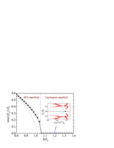
Figure 1: (color online) Phase diagram at $T=0$ (solid line) and $T=0.3T_{F}$ (gray dashed line), determined from the behavior of the lowest energy in quasiparticle spectrum. With increasing the effective Zeeman field, the Fermi cloud changes from a standard BCS superfluid to a topologically non-trivial superfluid. The phase transition point is slightly affected by finite temperature. The inset shows the energy spectrum at $h=1.2E_{F}$ as a function of the position of quasiparticles. A zero-energy quasiparticle (i.e., Majorana fermion) at the trap edge has been highlighted by a big dark circle. Here, we characterize approximately the position of a quasiparticle by using its wave-function: $\left\langle x^{2}\right\rangle=\int dxx^{2}\sum_{\sigma}[u_{\sigma}^{2}\left(x\right)+\nu_{\sigma}^{2}\left(x\right)]$.

Fig. 1 presents the phase diagram at these parameters and at two temperatures $T=0$ and $T=0.3T_{F}$, showing the well-known topological phase transition at a critical effective Zeeman field $h_{c}\simeq 1.05E_{F}$. The different phase is characterized by the lowest energy of Bogoliubov quasiparticles, $\min\{\left|E_{\eta}\right|\}$. At a small Zeeman field $h<h_{c}$, the system is a standard Bardeen-Cooper-Schrieffer (BCS) superfluid, with a fully gapped quasiparticle energy spectrum (i.e., $\min\{\left|E_{\eta}\right|\}>0$). Once $h>h_{c}$, however, topologically non-trivial phase emerges. Though the quasiparticle energy spectrum is still gapped in the bulk, gapless excitations - Majorana fermions - appear at the edges , leading to an exponentially small lowest energy in the spectrum. This is fairly evident in the inset, where we plot the energy spectrum as a function of the position of quasiparticles.

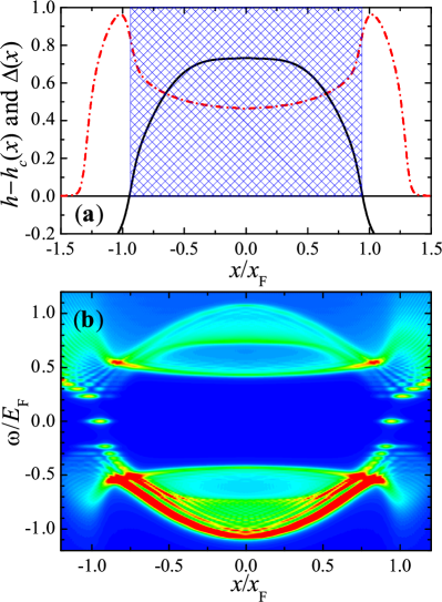
Figure 2: (color online) (a) The pairing gap distribution function $\Delta(x)$ (dot-dashed line) and the criterion for a local topological phase $h>h_{c}(x)$ (solid line) at $h=1.2E_{F}$. The shaded cross-hatching highlights the topologically non-trivial area. (b) The linear contour plot of the local density of state at $h=1.2E_{F}$. At each trap edge, a series of edge states, including the zero-energy Majorana fermion mode, are clearly visible.

To determine the critical Zeeman field $h_{c}$, we note that for a homogeneous spin-orbit coupled Fermi gas, it is given by Lutchyn2010 ; Oreg2010

$$h_{c}=\sqrt{\mu^{2}+\Delta^{2}}.$$ (30)

In harmonic traps as we consider here, the critical Zeeman field becomes position dependent. The local critical Zeeman field, calculated using $h_{c}(x)=\sqrt{\mu^{2}(x)+\Delta^{2}(x)}$, with the local chemical potential $\mu(x)=\mu-m\omega^{2}x^{2}/2$ and the local pairing gap $\Delta(x)$, increases monotonically towards the trap edge . The Fermi cloud at position $x$ will locally be in a topological state if the Zeeman field $h>h_{c}(x)$. For the parameters given in the above, this first happens at $h\simeq 1.05E_{F}$, for which the local phase at the trap center ($x=0$) starts to become topologically non-trivial. In Fig. 2(a), we show the local pairing gap $\Delta(x)$ and the criterion for a local topological state, $h>h_{c}(x)$, at the Zeeman field $h=1.2E_{F}$. At this field, the topological area is extended to the edge of the trap, as highlighted by a shaded cross-hatching. The appearance of Majorana fermion modes may be probed by measuring the local density of state through spatially resolved radio-frequency (rf) spectroscopy Liu2012 ; OurImpurity . In Fig. 2(b), we present the local density of state at $h=1.2E_{F}$,

$$\rho\left(x,\omega\right) = \frac{1}{2}\sum_{\sigma\eta}\left[\left|u_{\sigma\eta}\left(x\right)\right|^{2}\delta\left(\omega-E_{\eta}\right)\right.$$ (31)

$$+\left.\left|v_{\sigma\eta}\left(x\right)\right|^{2}\delta\left(\omega+E_{\eta}\right)\right].$$

At each of the two trap edges, we observe a series of edge states, whose dispersion relation is approximately given by Wei2012 , $E_{n}=\sqrt{n}\Delta E$, where $n=0,1,2,\cdots$ is a non-negative integer and $\Delta E$ is a characteristic energy scale set by the trapping frequency and recoil energy. The Majorana fermion modes with zero energy $E_{n}=0$ are clearly visible.

III Universal impurity-induced bound state

We are now ready to investigate how Bogoliubov quasiparticles are affected by a non-magnetic impurity. Hereafter, we focus on the topological state at $h=1.2E_{F}$. For a topologically trivial state at $h<1.05E_{F}$, we have checked numerically that quasiparticles are essentially not affected by the non-magnetic impurity scattering. This is in accord with the well-known Anderson’s theorem that potential scattering impurities are not pair-breakers in s-wave superconductors Balatsky2006 ; Anderson1959 .

III.1 Impurity-induced mid-gap state

In Fig. 3, we report the density profile and pairing gap distribution in the presence of a strong non-magnetic impurity with scattering potential strength, $V_{imp}=-0.30x_{F}E_{F}$. Both of them are completely depleted at the impurity site $x=0$. Accordingly, we observe the appearance of a new mid-gap state that is bound to the impurity, as shown in the inset for the spatial distribution of Bogliubov quasiparticles. This is clearly seen when we compare the quasiparticle spectrum without and with the non-magnetic impurity, i.e., the inset in Fig. 1 and Fig. 3, respectively. Away from the impurity site, the distribution of Bogoliubov quasiparticles is also disturbed by the impurity. However, the series of edge states at the trap edge seems to be very robust against the impurity scattering.

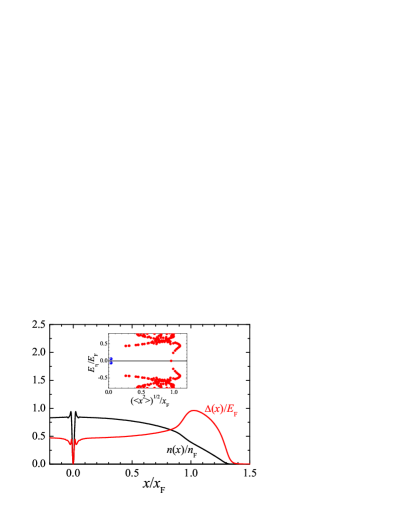
Figure 3: (color online) Density profile and pairing gap distribution in the presence of a strong attractive non-magnetic impurity with scattering potential strength, $V_{imp}=-0.30x_{F}E_{F}$. The inset shows the spatial distribution of Bogoliubov quasiparticle energy spectrum. The mid-gap bound state near the impurity site $x=0$ is highlighted by big blue circles.

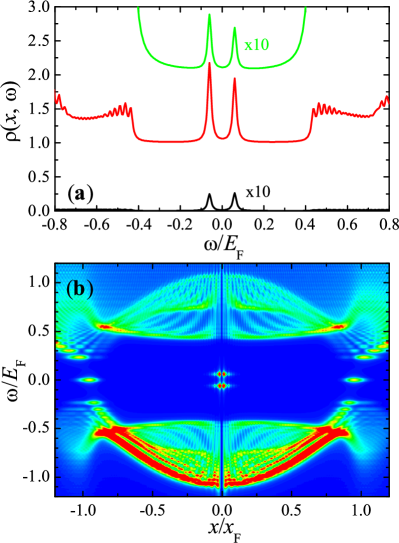
Figure 4: (color online) (a) Density of state for a topological superfluid ($h=1.2E_{F}$), at $x=0$, $0.05x_{F}$, and $0.1x_{F}$ (from bottom to top). For better illustration, the curves have been off-set. The magnitude of the local density of state at $x=0$ and $0.1x_{F}$ has been enlarged by a factor of $10$. (b) Linear contour plot of local density of state. The impurity induced bound state is clearly visible near $x=0$ and $\omega=0$.

In Fig. 4, we show the local density of state $\rho(x,\omega)$. The mid-gap bound state can be easily identified in spatially resolved rf spectroscopy, which is a cold-atom analog of scanning tunneling microscopy (STM). If such a bound state exists, one would observe a strong rf-signal at around origin and zero energy, which decays exponentially in space and energy. The maximum rf-signal, however, is located slightly away from the origin, as the total density is completely depleted right at the impurity site.

The existence of a mid-gap state in the topological superfluid phase is certainly not consistent with Anderson’s theorem Anderson1959 for potential scattering in s-wave superconductors. However, it can be understood from the combined effect of the spin-orbit coupling and effective Zeeman field. Beyond the critical Zeeman field $h_{c}$, the Fermi cloud is actually a p-wave-like superfluid (see, for example, the discussion in Sec. IIA of Ref. Wei2012 ). This is also the underlying reason why the cloud is in a topological state. For superfluids with a non-zero angular momentum order parameter, non-magnetic impurity is a pair-breaker and would lead to a mid-gap bound state.

III.2 Universal mid-gap state

An impurity-induced bound state is not a unique feature of topological superfluids, as it can also exist in superfluids with even-parity angular momentum order parameter, such as d-wave and g-wave superfluids. Here, however, we argue that the existence of a deep, universal in-gap bound state in the limit of strong impurity scattering would be a robust feature of topological superfluids. Despite of the details of impurity scattering (i.e., non-magnetic or magnetic impurity, positive or attractive scattering potential), we would observe exactly the same bound state, when the impurity scattering strength is strong enough. This argument is based on the consideration that a strong impurity will always deplete the atoms at the impurity site and hence create a vacuum area that is topologically trivial. Thus, at the interface between the topologically non-trivial and trivial areas, we would observe a pair of Majorana edge states Sau2012 - the precursor of the universal bound state. Ideally, the energy of the universal bound state will be zero.

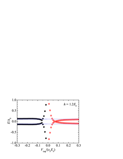
Figure 5: (color online) The dependence of the bound state energy on the impurity strength for a topological superfluid at $h=1.2E_{F}$. The solid and empty circles show the results for attractive and repulsive potential scattering, respectively. The dashed lines gives the bound state energy at the infinitely large impurity strength, $E\simeq\pm 0.113\Delta_{0}$, obtained by an extrapolation. Here, $\Delta_{0}\simeq 0.464E_{F}$ is the pairing gap at the trap center without impurity.

In Fig. 5, we plot the energy of the mid-gap bound state as a function of the impurity scattering strength at $h=1.2E_{F}$. Indeed, when the absolute value of the scattering strength $V_{imp}$ is sufficiently large, the energy of the bound state converges to a single value, $E\simeq 0.113\Delta_{0}$, where $\Delta_{0}\simeq 0.464E_{F}$ is the pairing gap at the trap center in the absence of impurity (see Fig. 3). We have also checked the case with a magnetic impurity and have found the same bound state energy (not shown in the figure). The same bound state energy, found under different type of strong impurities, is a clear indication of the emergence of a universal impurity-induced bound state. It would also be a unique feature of the existence of a topological superfluid.

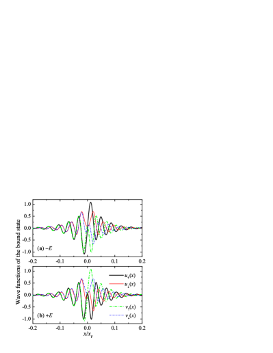
Figure 6: (color online) Wave-function of the universal bound state with energy $E\simeq\pm 0.113\Delta_{0}$, for a topological superfluid at $h=1.2E_{F}$. The wave-function at $\pm E$ may be regarded as the bond and anti-bond superposition of two Majorana wave-functions, which satisfy respectively the symmetry $u_{\sigma}\left(x\right)=\nu_{\sigma}^{*}\left(x\right)$ (on the left side with $x<0$) and $u_{\sigma}\left(x\right)=-\nu_{\sigma}^{*}\left(x\right)$ (on the right side with $x>0$).

We note, however, that the bound state energy is not precisely zero as we may anticipate from the Majorana edge-state picture as mentioned in the above. This is due to the fact that a pair of zero-energy Majorana fermions, localized at the same position (i.e., impurity site), could interfere with each other, leading to a small energy splitting whose magnitude would depend on the detailed configuration of the Fermi cloud. In Fig. 6, we present the wave-function of the universal impurity-induced bound state. Indeed, the wave-function of the universal bound state can be viewed as the bond and anti-bond superposition of the wave-functions of two Majorana fermions, which satisfy the symmetry of $u_{\sigma}\left(x\right)=\nu_{\sigma}^{*}\left(x\right)$ or $u_{\sigma}\left(x\right)=-\nu_{\sigma}^{*}\left(x\right)$, respectively.

We note also that the mid-gap state induced by non-magnetic impurities in topological superconducting nanowires has recently been predicted by Sau and Demler, based on a non-self-consistent T-matrix and Green function method Sau2012 . By increasing the impurity strength, it was reported that the bound state energy saturates to zero-energy, instead of converging to a nonzero value. In addition, a shallow bound state was predicted in the non-topological superconducting phase with spin-orbit coupling. These predictions are different from our numerical results. We ascribe these discrepancies to the lack of self-consistency in the T-matrix approach.

III.3 Realistic gaussian-shape impurity

We consider so far a delta-like impurity scattering potential. In real experiments, the non-magnetic impurity would be simulated by an off-resonant dimple laser light, which has a finite width in space. Thus, it is more reasonable to simulate the impurity by using a gaussian-shape scattering potential.

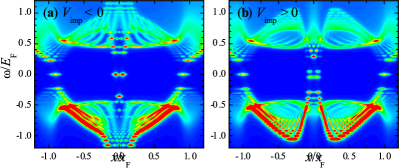
Figure 7: (color online) Linear contour plot of density of state at $h=1.2E_{F}$, for an attractive or a repulsive gaussian-shape impurity scattering potential. Here, we take $d=0.1x_{F}$ and $V_{imp}=\pm 0.30x_{F}E_{F}$.

Fig. 7 reports the linear contour plot of local density of state at $h=1.2E_{F}$ for a strong attractive (a) and repulsive (b) gaussian-shape impurity potential. With a finite width $d=0.1x_{F}$, we observe a series of bound states in the vicinity of the impurity site. The lowest-energy bound state is close to the universal bound state that we find earlier with a delta-like impurity potential.

To give some realistic parameters, let us consider a spin-orbit coupled Fermi gas of ⁴⁰K atoms confined to a tight 2D optical lattice, with an axial trapping frequency $\omega=2\pi\times 116$ Hz Wang2012 . By assuming the number of atoms $N=100$ in each tube, the Fermi energy or temperature is about $300$ nK. We may take $k_{F}\simeq 2k_{R}$ and a Raman strength $\Omega_{R}\simeq 10E_{R}$, where $E_{R}$ is the recoil energy. We may anticipate a topological superfluid at temperature $T<10$ nK. The typical size of the Fermi cloud is about $x_{F}\simeq 15$ $\mu m$. Thus, we may use an off-resonant dimple laser with width $d\simeq 1.5$ $\mu m$ to simulate the non-magnetic impurity. The strength of the impurity can be easily tuned by controlling the strength of the dimple laser light. With these parameters, we may be able to observe the universal impurity-induced bound state discussed in the above.

IV Conclusions

In summary, we have argued that a strong non-magnetic impurity will induce a universal bound state in topological superfluids. This provides a unique feature to characterize the long-sought topological superfluids. We have proposed a realistic setup to observe such a universal impurity-induced bound state in atomic topological superfluids, which are to be realized in spin-orbit coupled Fermi gases of ⁴⁰K atoms. The necessary conditions, including the realization of spin-orbit coupling by two-photon Raman process, the achievement of one-dimensional confinement by optical lattice, and the simulation of non-magnetic impurities using off-resonant dimple laser light, are all within the current experimental reach. Therefore, we anticipate our proposal will be realized soon at Shanxi University in China Wang2012 or elsewhere.

Appendix A Solving the BdG equation in one dimension

We solve the BdG equation Eq. (26) by expanding the Bogoliugbov wavefunctions $u_{\sigma}(x)$ and $\nu_{\sigma}(x)$ in the basis of 1D harmonic oscillators $\phi_{j}(x)=(1/\sqrt{\pi^{1/2}2^{j}j!})H_{j}(x)e^{-x^{2}/2}$,

$$u_{\sigma}\left(x\right) = \sum_{j=0}^{M-1}U_{\sigma j}\phi_{j}\left(x\right),$$ (32)

$$\nu_{\sigma}\left(x\right) = \sum_{j=0}^{M-1}V_{\sigma j}\phi_{j}\left(x\right),$$ (33)

Here, $H_{j}(x)$ is the $j$-th Hermite polynomial and, for convenience, we have used the natural unit in harmonic traps, $m=\hbar=\omega=1$, so that the oscillator length $a\equiv\sqrt{\hbar/(m\omega)}=1$ and the oscillator energy $\hbar\omega=1$. On such a basis, the BdG Hamiltonian Eq. (22) is converted to a $4M\times 4M$ secular matrix,

$${\cal H}_{BdG}=\left[\begin{array}[]{cccc}{\cal H}_{S}^{ij}-h\delta_{ij}&-R_{ij}&0&-\Delta_{ij}\\ R_{ij}&{\cal H}_{S}^{ij}+h\delta_{ij}&\Delta_{ij}&0\\ 0&\Delta_{ij}&-{\cal H}_{S}^{ij}+h\delta_{ij}&R_{ij}\\ -\Delta_{ij}&0&-R_{ij}&-{\cal H}_{S}^{ij}-h\delta_{ij}\end{array}\right],$$ (34)

where the matrix elements,

$${\cal H}_{S}^{ij} = \left(i+1/2-\mu\right)\delta_{ij}+V_{imp}^{ij},$$ (35)

$$R_{ij} = \lambda\left[\sqrt{j/2}\delta_{i,j-1}-\sqrt{\left(j+1\right)/2}\delta_{i,j+1}\right].$$ (36)

To calculate efficiently the matrix elements $V_{imp}^{ij}\equiv\int_{-\infty}^{+\infty}dx\phi_{i}(x)V_{imp}(x)\phi_{j}(x)$ and $\Delta_{ij}\equiv\int_{-\infty}^{+\infty}dx\phi_{i}(x)\Delta(x)\phi_{j}(x)$, we discretize space $(-L/2,L/2)$ into $N_{grid}$ equally spaced points, where the simulation length $L$ and the number of grid $N_{grid}$ should be sufficiently large so that the basis function $\phi_{j}(x)$ ($j=0,..,M-1$) can be accurately sampled. At the number of atoms $N=100$, typically we take $M=500$, $N_{grid}=6400$, and $L=70\sqrt{\hbar/(m\omega)}$. The gaussian impurity potential $V_{imp}\left(x\right)$ and pairing gap function $\Delta\left(x\right)$, as well as the total density $n(x)$, will be stored as an array of length $N_{grid}$. We note that, for a delta-like impurity we immediately have $V_{imp}^{ij}=V_{imp}\phi_{i}\left(x_{0}\right)\phi_{j}\left(x_{0}\right)$. By diagonalizing the $4M\times 4M$ secular matrix Eq. (34), we obtain the quasiparticle energy $E_{\eta}$ and the eigenvector $U_{\sigma j}^{\eta}$ and $V_{\sigma j}^{\eta}$ ($j=0,..,M-1$). The latter gives the quasiparticle wave-function $u_{\sigma\eta}\left(x\right)$ and $\nu_{\sigma\eta}\left(x\right)$. Note that, the eigenvector $U_{\sigma j}^{\eta}$ and $V_{\sigma j}^{\eta}$ have to satisfy the condition $\sum_{\sigma j}[(U_{\sigma j}^{\eta})^{2}+(V_{\sigma j}^{\eta})^{2}]=1$, due to the normalization of the quasiparticle wavefunctions, i.e., $\int_{-\infty}^{+\infty}dx\sum_{\sigma}[u_{\sigma\eta}^{2}(x)+v_{\sigma\eta}^{2}(x)]=1$.

In the practical calculation, due to computational limitation, we have to use a finite expansion basis. This is controlled by the cut-off $M$ for the number of 1D harmonic oscillators. Furthermore, we must impose a high energy cut-off $E_{c}$ for the quasiparticle energy levels. To make our result cut-off independent, we adopt a hybrid approach, in which we solve the discrete BdG equation for the energy levels below the high energy cut-off $E_{c}$. While above $E_{c}$, we use a semiclassical plane-wave approximation for the wavefunctions that should work very well for high-lying energy levels. For simplicity, to take the semiclassical approximation we may neglect the spin-orbit coupling term $R_{ij}$ in the BdG Hamiltonian Eq. (34). In the end, for the pairing gap function and the total density, we shall use the semiclassical expressions listed in the Sec. IVC of Ref. Liu2007 . To summarize briefly, the contributions of discrete low-lying energy levels (labeled by an index “$\eta$”) and continuous high-lying energy levels to the total density are given by,

$$n_{d}\left(x\right)=\frac{1}{2}\sum_{\left|E_{\eta}\right|<E_{c}}\sum_{\sigma}\left[\left|u_{\sigma\eta}\left(x\right)\right|^{2}f\left(E_{\eta}\right)+\left|v_{\sigma\eta}\left(x\right)\right|^{2}f\left(-E_{\eta}\right)\right]$$ (37)

and

$$n_{c}\left(x\right)=\frac{\sqrt{2m}}{4\pi\hbar}\left(\int\limits_{E_{c}+h}^{+\infty}+\int\limits_{E_{c}-h}^{+\infty}\right)d\epsilon\frac{\left[\epsilon/\sqrt{\epsilon^{2}-\Delta^{2}\left(x\right)}-1\right]}{\sqrt{\mu+\sqrt{\epsilon^{2}-\Delta^{2}\left(x\right)}}},$$ (38)

respectively. For the pairing gap function, we have

$$\Delta(x)=-\frac{g_{1D}^{eff}\left(x\right)}{2}\sum_{\left|E_{\eta}\right|<E_{c}}\sum_{\sigma}\left[u_{\uparrow\eta}\left(x\right)v_{\downarrow\eta}^{*}\left(x\right)f\left(E_{\eta}\right)+u_{\downarrow\eta}\left(x\right)v_{\uparrow\eta}^{*}\left(x\right)f\left(-E_{\eta}\right)\right],$$ (39)

where the effective interaction strength $g_{1D}^{eff}\left(x\right)$ is determined by,

$$\frac{1}{g_{1D}^{eff}\left(x\right)}=\frac{1}{g_{1D}}+\frac{\sqrt{2m}}{4\pi\hbar}\int\limits_{E_{c}-h}^{\infty}d\epsilon\frac{1}{\sqrt{\epsilon^{2}-\Delta^{2}\left(x\right)}}.$$ (40)

The numerical procedure of solving the BdG equation is therefore as follows. For a given set of parameters ($N$, $g_{1D}$, $h$, $\lambda$, and $T$), we (1) start with an initial guess or a previously determined better estimate for $\Delta\left(x\right)$, (2) solve Eq. (40) for the effective coupling constant, (3) then solve Eq. (34) for all the quasiparticle wavefunctions up to the chosen energy cut-off to find $u_{\sigma\eta}\left(x\right)$ and $v_{\sigma\eta}\left(x\right)$, and finally determine an improved value for the order parameter from Eq. (39). During the iteration, the total density $n(x)=n_{d}(x)+n_{c}(x)$ is updated. The chemical potentials $\mu$ is adjusted slightly in each iterative step to enforce the number-conservation condition $\int_{-\infty}^{+\infty}dxn(x){\bf=}N$, until final convergence is reached.

A.1 Check on the numerical accuracy

We have checked carefully the numerical accuracy of our hybrid approach at different sets of parameters and at both zero temperature and finite temperatures. In Fig. 8, we check the dependence on the cut-off energy $E_{c}$ at $h=1.2E_{F}$ in the absence of impurity scattering. The pairing gap function becomes essentially independent on $E_{c}$ once $E_{c}\geq 6E_{F}$, with a relative error less than $1$%. The cut-off energy dependence for the total density is even weaker (not shown in the figure). Thus, we conclude that our hybrid calculation is quantitatively reliable with $E_{c}=6E_{F}$. At this energy cut-off, each iteration in the self-consistent calculation takes approximately several minutes, by using a standard desktop computer. The convergence for a set of parameters is typically reached after $20-50$ iterations.

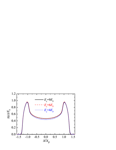
Figure 8: (color online) The dependence of the pairing gap function on the high-energy cut-off $E_{c}$. Here, we consider a spin-orbit coupled Fermi gas of $N=100$ atoms in harmonic traps at zero temperature. The dimensionless interaction parameter is $\gamma=\pi$. The spin-orbit coupling is taken to be $\lambda k_{F}/E_{F}=1$ and $h=1.2E_{F}$. At these typical parameters, the results become independent on the cut-off energy $E_{c}$ once it is larger than $6E_{F}$.

References

• (1) A. V. Balatsky, I. Vekhter, and J.-X. Zhu, Rev. Mod. Phys. 78, 373 (2006).
• (2) A. P. Mackenzie, R. K. W. Haselwimmer, A. W. Tyler, G. G. Lonzarich, Y. Mori, S. Nishizaki, and Y. Maeno, Phys. Rev. Lett. 80, 161 (1998).
• (3) A. J. Millis, Solid State Commun. 126, 3 (2003).
• (4) X.-L. Qi and S.-C. Zhang, Rev. Mod. Phys. 83, 1057 (2011).
• (5) E. Majorana, Nuovo Cimennto 14, 171 (1937).
• (6) F. Wilczek, Nat. Phys. 5, 614 (2009).
• (7) A. Kitaev, Ann. Phys. (NY) 321, 2 (2006).
• (8) C. Nayak, S. Simon, A. Stern, M. Freedman, and S. Das Sarma, Rev. Mod. Phys. 80, 1083 (2008).
• (9) V. Mourik, K. Zuo, S. M. Frolov, S. R. Plissard, E. P. A. M. Bakkers, and L. P. Kouwenhoven, Science 336, 1003 (2012).
• (10) L. P. Rokhinson, X. Liu, and J. K. Furdyna, arXiv:1204.4214 (2012).
• (11) A. Das, Y. Ronen, Y. Most, Y. Oreg, M. Heiblum, and H. Shtrikman, arXiv:1205.7073 (2012).
• (12) L. Fu and C. L. Kane, Phys. Rev. Lett. 100, 096407 (2008).
• (13) J. Alicea, Y. Oreg, G. Refael, F. von Oppen and M. P. A. Fisher, Nature Phys. 7, 412 (2011).
• (14) L. Jiang, T. Kitagawa, J. Alicea, A. R. Akhmerov, D. Pekker, G. Refael, J. I. Cirac, E. Demler, M. D. Lukin, and P. Zoller, Phys. Rev. Lett. 106, 220402 (2011).
• (15) X.-J. Liu and H. Hu, Phys. Rev. A 85, 033622 (2012).
• (16) R. Wei and E. J. Mueller, arXiv:1208.5450 (2012).
• (17) I. Bloch, J. Dalibard, and W. Zwerger, Rev. Mod. Phys. 80, 885 (2008).
• (18) C. Chin, R. Grimm, P. Julienne, and E. Tiesinga, Rev. Mod. Phys. 82, 1225 (2010).
• (19) H. Hu, X.-J. Liu, and P. D. Drummond, Phys. Rev. Lett. 98, 070403 (2007).
• (20) Y. A. Liao, A. S. C. Rittner, T. Paprotta, W. Li, G. B. Partridge, R. G. Hulet, S. K. Baur, and E. J. Mueller, Nature (London) 467, 567 (2010).
• (21) P. Wang, Z.-Q. Yu, Z. Fu, J. Miao, L. Huang, S. Chai, H. Zhai and J. Zhang, Phys. Rev. Lett. 109, 095301 (2012).
• (22) L. W. Cheuk, A. T. Sommer, Z. Hadzibabic, T. Yefsah, W. S. Bakr, and M. W. Zwierlein, Phys. Rev. Lett. 109, 095302 (2012).
• (23) L. Jiang, L. O. Baksmaty, H. Hu, Y. Chen, and H. Pu, Phys. Rev. A 83, 061604(R) (2011).
• (24) L. Sanchez-Palencia and M. Lewenstein, Nature Phys. 6, 87 (2010).
• (25) J. D. Sau and E. Demler, arXiv:1204.2537 (2012).
• (26) Z. Yan, X. Yang, L. Sun, and S. Wan, arXiv:1204.0571 (2012).
• (27) T. Bergeman, M. G. Moore, and M. Olshanii, Phys. Rev. Lett. 91, 163201 (2003).
• (28) X.-J. Liu, H. Hu, and P. D. Drummond, Phys. Rev. A 76, 043605 (2007).
• (29) X.-J. Liu, H. Hu, and P. D. Drummond, Phys. Rev. A 78, 023601 (2008).
• (30) R. M. Lutchyn, J. D. Sau, and S. D. Sarma, Phys. Rev. Lett. 105, 077001 (2010).
• (31) Y. Oreg. G. Refael, and F. von Oppen, Phys. Rev. Lett. 105, 177002 (2010).
• (32) P. W. Anderson, J. Phys. Chem. Solids 11, 26 (1959).