Variational theory of soliplasmon resonances

Abstract

We present a first-principles derivation of the variational equations describing the dynamics of the interaction of a spatial soliton and a surface plasmon polariton (SPP) propagating along a metal/dielectric interface. The variational ansatz is based on the existence of solutions exhibiting differentiated and spatially resolvable localized soliton and SPP components. These states, referred to as soliplasmons, can be physically understood as bound states of a soliton and a SPP. Their respective dispersion relations permit the existence of a resonant interaction between them, as pointed out in Bliokh_PRA_2009 . The existence of soliplasmon states and their interesting nonlinear resonant behavior has been validated already by full-vector simulations of the nonlinear Maxwell’s equations, as reported in Milian_OL_2012 . Here, we provide the theoretical demonstration of the nonlinear resonator model previously introduced in our previous work and analyze all the approximations needed to obtain it. We also provide some extensions of the model to improve its applicability.

I Introduction

The idea that a spatial soliton and a surface plasmon polariton (SPP) can couple to form the soliton-plasmon, or soliplasmon, bound state was originally proposed in Ref. Bliokh_PRA_2009 . These authors proposed by means of a sharp physical intuition that the bound system should obey in certain limit a nonlinearly coupled oscillator model with a peculiar nonlinearity, originated by the soliton tail at the metal interface, which was considered as the driving mechanism for the coupling and the dynamical features of the soliplasmon system. Despite the amount of undetermined coefficients in the model, relevant qualitative predictions of the soliplasmon properties were made. These nonlinear modes where later numerically demonstrated to exist in the context of the general vectorial nonlinear Maxwell equations and the nonlinear oscillator model (found with asymmetric coupling) was presented with fully determined coefficients Milian_OL_2012 . However, that oscillator model was never proved.

Although the soliplasmon proposal is relatively recent, monochromatic surface waves in the vicinity of the interface between a nonlinear dielectric and a metal were extensively studied during the decade of the 80’s by many authors (see, to cite only a few, Agranovich_JETP_1980 ; Tomlinson_OL_1980 ; Akhmediev_JETP_1982 ; Yu1983a ; Leung_PRB_1985 ; Mihalache_PS_1984 ; Stegeman1985a ; Ariyasu_JAP_1985 ). Amongst those theoretical results, corrections to the profile and wavenumber of i) SPP’s due to nonlinearity and ii) of the spatial solitons due to the presence of a metallic interface far from its core, were presented. At that time, none of the studies, to the best of our knowledge, considered simultaneously a spatial soliton and a SPP; the two component wave referred to as soliplasmon. Recently, the model presented in Ariyasu_JAP_1985 has been extended in a first attempt to describe soliplasmons in the challenging and more realistic 2D geometry, consisting of several interfaces Walasik_OL_2012 . So far the 2D symmetric like modes are reported, but the antisymmetric ones, which in principle require less power in the soliton component Milian_OL_2012 , remain unfound. On the other hand, the role of nonlinear vector effects, generated by strong gradients of the effective nonlinearly induced refractive index, can be of relevance for understanding soliplasmon modes near resonance or with high plasmonic component, such as in metals directly attached to the nonlinear medium, so standard scalar soliton solutions cannot be appropriate when they are too close to the interface and a full-vector soliton solution is required Ciattoni2005a .

In this paper, we present the detailed derivation of the nonlinear oscillator model from first principles. We focus on 1D soliplasmons in two geometries of interest, namely the metal/Kerr (MK) Milian_OL_2012 and the metal/dielectric/Kerr (MDK) Bliokh_PRA_2009 interfaces (by dielectric we implicitly mean a linear dielectric and by a Kerr dielectric with cubic nonlinearity). The paper is organized as follows: in Section II, we motivate and present our variational ansatz and the main features of soliton-plasmon coupling in the general context of nonlinear Maxwell’s equations; in Section III, we focus on the soliton component of the soliplasmon ansatz in the case of total decoupling and we obtain the dynamical equation for the soliton variational parameter; in Section IV, we obtain the equation for a general nonlinear plasmon stationary mode (decoupled from soliton) and construct the dynamical equation for the plasmon variational parameter. Finally, in Section V, we obtain the nonlinear resonator model for the coupled system formed by a nonlinear plasmon and a soliton in the weak coupling approximation. In Section VI, we pay attention to the cases of a MK and MDK geometries previous mentioned recovering and demonstrating the model presented in Refs.Bliokh_PRA_2009 ; Milian_OL_2012 . In all sections, we stress the role played by the different approximations used in our derivation. The relevance and differences of this model with respect other approaches are especially emphasized in the conclusions.

II Variational ansatz for nonlinear Maxwell’s equations

We consider the wave equation for the electric component of a monochromatic EM field describing its propagation in an optical media characterized by inhomogeneous linear and nonlinear (Kerr) susceptibilities. We take the most general form of these equations derived from Maxwell’s equations without assuming neither the scalar nor the paraxial approximations. Thus, our starting point is:

$$\nabla^{2}\mathbf{E}-\nabla\left(\nabla\cdot\mathbf{E}\right)=-k_{0}^{2}\mathbf{D}\left(\mathbf{E}\right)=-k_{0}^{2}\varepsilon_{L}\mathbf{E}-k_{0}^{2}\mathbf{P}_{\mathrm{NL}}\left(\mathbf{E}\right)$$ (1)

where $\varepsilon_{L}(\mathbf{x})\equiv 1+\chi^{(1)}(\mathbf{x)}$ is the in-homogenous linear dielectric function and

$$\mathbf{P}_{\mathrm{NL}}\left(\mathbf{E}\right)=\chi^{(3)}\left(\mathbf{E}\cdot\mathbf{E}^{*}\right)\mathbf{E}+\bar{\chi}^{(3)}\left(\mathbf{E}\cdot\mathbf{E}\right)\mathbf{E}^{*},$$

is the Kerr nonlinear polarization, where $\chi^{(3)}(\mathbf{x})$ and $\bar{\chi}^{(3)}(\mathbf{x})$ are the in-homogeneous third order susceptibilities associated to the Kerr effect. All functions have an implicit, but undisplayed, dependence on the frequency of the nonlinear wave $\omega=ck_{0}$.

Our goal is to find a simplified, although physically meaningful, model describing the existence of soliton-plasmon resonances, or soliplasmons, obtained by the interaction of a spatial soliton of the Kerr medium with a Surface Plasmon Polariton (SPP) on a metal/dielectric interface. We consider a simple configuration consisting in a spatial soliton moving (within a Kerr medium) in parallel to a metal/dielectric interface interacting with a SPP propagating on it (see Fig.1). It has been proven that stationary nonlinear states of this system in the form of soliton-plasmon resonances indeed exists as a solution of Eq.(1) for this type of configuration Milian_OL_2012 . They show a structure in which the soliton and plasmon components are clearly distinguishable, which supports to adopt the following variational ansatz:

$$\mathbf{E}=\mathbf{E}_{\mathrm{np}}\left[\left\{A_{i}(z)\right\}_{i=1}^{N}\right]+\mathbf{E}_{s}\left[\left\{C_{i}(z)\right\}_{i=1}^{N}\right],$$ (2)

in which, in principle, we do not explicitly display the dependence on the variational parameters so that a multi-parametric dependence can be assumed. We will particularize these parameters later. We also allow the SPP to behave nonlinearly by the effect of the Kerr nonlinearity on its own propagation Agranovich_JETP_1980 ; Davoyan_OE_2009 thus giving rise to what we call a nonlinear plasmon. We introduce the general ansatz (2) in Eq. (1) to get:

$$\frac{\partial^{2}\mathbf{E}_{\mathrm{np}}}{\partial z^{2}}+L_{0}\mathbf{E}_{\mathrm{np}}-\nabla\left(\nabla\cdot\mathbf{E}_{\mathrm{np}}\right)+\frac{\partial^{2}\mathbf{E}_{s}}{\partial z^{2}}+L_{0}\mathbf{E}_{s} =$$

$$=-k_{0}^{2}\mathbf{P}_{\mathrm{NL}}\left(\mathbf{E}_{\mathrm{np}}\right)-k_{0}^{2}\mathbf{P}_{\mathrm{NL}}\left(\mathbf{E}_{\mathrm{s}}\right)-k_{0}^{2}\mathbf{Q}_{\mathrm{K}}\left(\mathbf{E}_{\mathrm{np}},\mathbf{E}_{\mathrm{s}}\right),$$ (3)

where we have taken into account that the soliton is essentially a scalar solution so that $\nabla\cdot\mathbf{E}_{s}\approx 0$. We have also defined the differential operator $L_{0}$ as $L_{0}\equiv\nabla_{t}^{2}+k_{0}^{2}\varepsilon_{L}$ where $\nabla_{t}=\left(\partial_{x},\partial_{y}\right)$ is the transverse gradient operator. The term $\mathbf{Q}_{\mathrm{K}}\left(\mathbf{E}_{\mathrm{np}},\mathbf{E}_{\mathrm{s}}\right)$ includes all nonlinear Kerr terms coupling the SPP and soliton components:

$$\mathbf{Q}_{\mathrm{K}}\left(\mathbf{E}_{\mathrm{np}},\mathbf{E}_{\mathrm{s}}\right)\equiv\mathbf{P}_{\mathrm{NL}}\left(\mathbf{E}_{\mathrm{np}}+\mathbf{E}_{s}\right)-\mathbf{P}_{\mathrm{NL}}\left(\mathbf{E}_{\mathrm{np}}\right)-\mathbf{P}_{\mathrm{NL}}\left(\mathbf{E}_{\mathrm{s}}\right).$$ (4)

The SPP and soliton fields have different features. The SPP, as a surface wave and even when it behaves nonlinearly, can only exist bounded to the metal/dielectric interface, its nature being purely vectorial. On the other hand, the soliton can move freely in the Kerr medium with no restriction and its existence is due to the Kerr nonlinearity and it is essentially a scalar wave. It is clear from physical arguments and from results in Ref.Milian_OL_2012 that the coupling between these two entities vanishes as we move the soliton far way from the interface. In such a case, the overlapping of $\mathbf{E}_{\mathrm{np}}$ and $\mathbf{E}_{s}$ tends to zero and, thus, $\mathbf{Q}_{\mathrm{K}}\rightarrow 0$. In the limiting case in which they are infinitely far away, Eq.(1) gives rise to two independent equations for $\mathbf{E}_{\mathrm{np}}$ and $\mathbf{E}_{s}$:

$$\frac{\partial^{2}\mathbf{E}_{\mathrm{np}}}{\partial z^{2}}+L_{0}\mathbf{E}_{\mathrm{np}}-\nabla\left(\nabla\cdot\mathbf{E}_{\mathrm{np}}\right)=-k_{0}^{2}\mathbf{P}_{\mathrm{NL}}\left(\mathbf{E}_{\mathrm{np}}\right)$$ (5)

and

$$\frac{\partial^{2}\mathbf{E}_{s}}{\partial z^{2}}+L_{0}\mathbf{E}_{s}=-k_{0}^{2}\mathbf{P}_{\mathrm{NL}}\left(\mathbf{E}_{\mathrm{s}}\right).$$ (6)

Thus we can consider the action of $\mathbf{Q}_{\mathrm{K}}$ as a perturbation that couples the solutions of these two independent equations. For this reason, in our variational approach we will first consider the situation in which the two previous equations are satisfied separately. We will write the variational equations for both components separately and then we introduce the first order correction originated by the coupling term $\mathbf{Q}_{\mathrm{K}}$ .

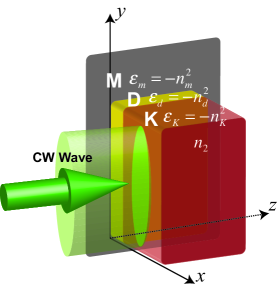
Figure 1: Parallel illumination of a metal/dielectric interface from a Kerr medium.

III Variational equation for the soliton

We start by considering the equation of an uncoupled soliton field satisfying Eq.(6). We consider the simplest case by choosing the fundamental soliton solution as a variational ansatz and by taking a single variational parameter, namely, the soliton amplitude. In the planar geometry under consideration, as given by Fig.1, we consider a $x$ and $z$ dependence only, so that the fundamental soliton corresponds to that of the 1D Helmholtz equation. This stationary solution has the sech form:

$$\mathbf{\bar{E}}_{\mathrm{s}}(x,z)=\mathbf{u}C\mathrm{sech}\left[\sqrt{\frac{\gamma}{2}}k_{0}C\left(x-a\right)\right]e^{i\beta_{s}z}\equiv\mathbf{u}\bar{E}_{s}(x;C)e^{i\beta_{s}z},\,\,\,\,\,\,C\in\mathbb{R}^{+},\,\,\,a\text{$\in$}\mathbb{R}^{+},$$ (7)

where $\gamma=\chi^{(3)}+\bar{\chi}^{(3)}$, $\mathbf{u}$ is a real unitary vector and the propagation constant of the soliton is given by

$$\beta_{s}^{2}=k_{0}^{2}\left(\varepsilon_{\mathrm{K}}+\frac{\gamma}{2}C^{2}\right),$$

$\varepsilon_{\mathrm{K}}$ being the linear dielectric constant of the Kerr medium. It is easy to check that the expression (7) verifies:

$$\left[\nabla_{t}^{2}+k_{0}^{2}\left(\varepsilon_{\mathrm{K}}+\gamma\left|\mathbf{\bar{E}}_{\mathrm{s}}\right|^{2}\right)\right]\bar{\mathbf{E}}_{\mathrm{s}}=\beta_{s}^{2}\mathbf{\bar{E}}_{\mathrm{s}},$$ (8)

or, equivalently, Eq.(6) for a stationary solution in which $\mathbf{P}_{\mathrm{NL}}=\gamma\left|\mathbf{\bar{E}}_{\mathrm{s}}\right|^{2}\mathbf{\bar{E}}_{\mathrm{s}}$.

Now, we make the ansatz for the soliton component. As shown in Ref.Milian_OL_2012 , for quasi-stationary evolution the dynamics of the soliton position $a$ is much slower than that of the amplitude. For this reason, we promote the soliton amplitude $C$ to the category of the only variational parameter for the case under consideration. Therefore, we establish the ansatz as follows:

$$\mathbf{\bar{E}}_{s}(x,z)\rightarrow\mathbf{E}_{s}(x,z)=\mathbf{u}C(z)\mathrm{sech}\left[\sqrt{\frac{\gamma}{2}}k_{0}\left|C(z)\right|\left(x-a\right)\right]\,\,\,\,\,\,C(z)\in\mathbb{C}.$$ (9)

Our aim now is to find the dynamical equation for the variational parameter $C(z)$. We immediately recognize that the previous ansatz admits the following useful decomposition (taking into account that we can write $C(z)=\left|C(z)\right|\exp\left[i\varphi_{s}(z)\right]$):

$$\mathbf{E}_{s}(x,z)=\mathbf{u}e^{i\varphi_{s}(z)}\bar{E}_{s}(x;|C(z)|),$$

where $\bar{E}_{s}(x;|C(z)|)$ is the stationary soliton solution characterized by the real and positive amplitude $|C(z)|$ and, consequently, by a propagation constant $\beta_{s}=k_{0}\left(\varepsilon_{\mathrm{K}}+\frac{\gamma}{2}|C\left(z\right)|^{2}\right)^{1/2}$. Since we are interested in quasi-stationary evolution, we will assume that the dynamics of $|C(z)|$ is much slower than that of the corresponding phase $\varphi_{s}(z)$, so that, $d|C|/dz\ll d\varphi_{s}/dz$. This assumption is supported by numerical simulations Milian_OL_2012 . We substitute now the ansatz Eq.(9) into the soliton wave equation (6):

$$\frac{\partial^{2}\mathbf{E}_{s}}{\partial z^{2}}+L_{0}\mathbf{E}_{s}=-k_{0}^{2}\left[\left(\chi^{(3)}+\bar{\chi}^{(3)}\right)\left|\mathbf{E}_{s}\right|^{2}\right]\mathbf{E}_{s},$$

which can be written as

$$\frac{\partial^{2}\mathbf{E}_{s}}{\partial z^{2}}+\left[\nabla_{t}^{2}+k_{0}^{2}\left(\varepsilon_{\mathrm{K}}+\gamma\left|\mathbf{E}_{\mathrm{s}}\right|^{2}\right)\right]\mathbf{E}_{\mathrm{s}}=0.$$ (10)

But, since according to our ansatz, $\mathbf{E}_{s}(x,z)=\mathbf{u}\exp\left[i\varphi_{s}(z)\right]\bar{E}_{s}(x,z)\equiv\mathbf{u}E_{s}(x,z)$, we can see that the differential operator in brackets only acts on the stationary solution $\bar{E}_{s}$. Since the latter field, on the other hand, satisfies the stationary equation (8), this means that the variational field $\mathbf{E}_{s}$ also fulfills

$$\left[\nabla_{t}^{2}+k_{0}^{2}\left(\varepsilon_{\mathrm{K}}+\gamma\left|\mathbf{E}_{\mathrm{s}}\right|^{2}\right)\right]\mathbf{E}_{\mathrm{s}}=\beta_{s}^{2}\mathbf{E}_{\mathrm{s}},$$ (11)

and, therefore, the previous equation becomes:

$$\frac{\partial^{2}E_{s}\left(x;C(z)\right)}{\partial z^{2}}+\beta_{s}^{2}E_{\mathrm{s}}\left(x;C(z)\right)=0.$$

At this point, we introduce another useful decomposition for the variational field (9): $E_{s}(x,z)=C(z)f_{s}(x;|C(z)|)$, where $f_{s}=\mathrm{sech}\left[\sqrt{\frac{\gamma}{2}}k_{0}\left|C(z)\right|\left(x-a\right)\right].$ This decomposition permits to write the equation above as:

$$\frac{\partial^{2}}{\partial z^{2}}\left[C(z)f_{s}(x;|C(z)|\right]+\beta_{s}^{2}\left[C(z)f_{s}(x;|C(z)|\right]=0.$$

In order to obtain a dynamical equation for $C(z)$, we need to project the previous equation with respect to a suitable function. A natural choice for the projection function is the stationary soliton solution at the initial propagation point, i.e., $\bar{E}_{s}(0)=C(0)f_{s}(x;|C(0)|)$. Since $C(0)$ is constant, it disappears in the projection process, so that, after projection we have:

$$\frac{d^{2}}{dz^{2}}\left[C(z)\int_{\mathbb{R}}f_{s}\left(x,0\right)f_{s}(x;|C(z)|)\right]+\beta_{s}^{2}\left[C(z)\int_{\mathbb{R}}f_{s}\left(x,0\right)f_{s}(x;|C(z)|)\right]=0.$$

We introduce now the notation $N_{s}\equiv\int_{\mathbb{R}}f_{s}(0)f_{s}(z)$ and we immediately recognize that the dependence of $N_{s}$ on $z$ comes exclusively from its dependence on the modulus of the soliton amplitude $|C(z)|$. However, due to the quasi-stationary approximation $d|C|/dz\ll d\varphi_{s}/dz$,

$$\frac{d^{2}}{dz^{2}}\left[C(z)N_{s}\left(|C(z)|\right)\right]\approx\left(\frac{d^{2}C(z)}{dz^{2}}\right)N_{s}\left(|C(z)|\right).$$ (12)

Therefore, the variational equation for the soliton parameter takes the simple form:

$$N_{s}\left[\frac{d^{2}}{dz^{2}}C(z)+\beta_{s}^{2}\left(|C|\right)C(z)\right]=0.$$

IV Variational equation for the nonlinear plasmon

In the case of the nonlinear plasmon component, we follow a similar procedure as for the soliton case. However, equations are here more cumbersome to analyze since we have to deal with the vectorial part of the differential operator in the wave equation (5). Another difference is that, since the SPP is a surface wave, the linear dielectric function is no longer a constant, as for the soliton equation, but rather a function defining the dielectric/metal interface:

$$\varepsilon_{L}(x)=\varepsilon_{p}(x)\equiv\begin{cases}\varepsilon_{m}&\mathrm{if\,\,}x\leq 0\\ \varepsilon_{d}&\mathrm{if\,\,}x>0.\end{cases}$$ (13)

A nonlinear plasmon is a stationary solution of Eq.(5) of the form:

$$\mathbf{\bar{E}}_{\mathrm{np}}(x,z)=\mathbf{e}_{\mathrm{np}}(x)e^{i\beta_{\mathrm{np}}z}=\left(\begin{array}[]{c}\mathbf{e}_{\mathrm{np}t}(x)\\ e_{\mathrm{np}z}(x)\end{array}\right)e^{i\beta_{\mathrm{np}}z},$$

where $\mathbf{e}_{\mathrm{np}t}=\left(e_{\mathrm{np}x},e_{\mathrm{np}y}\right)^{\top}$ stands for the transverse components of the electric field. We will consider that the nonlinear plasmon stationary solution is a conservative soliton. This means that for the stationary solution we will assume that the system has no losses, neither linear nor nonlinear, so that $\varepsilon_{L}$ will be a real function. For the same reason, we will take real nonlinear susceptibilities ($\chi^{(3)},\bar{\chi}^{(3)}\in\mathbb{R}$ ). The complex character of a realistic $\varepsilon_{L}$ will be taken into account when we set the dynamical equations for the variational solution.

According to Eq.(5), the transverse components of the nonlinear plasmon solution verify:

$$-\beta_{\mathrm{np}}^{2}\mathbf{e}_{\mathrm{np}t}+\nabla^{2}\mathbf{e}_{\mathrm{np}t}-\nabla_{t}\left(i\beta_{\mathrm{np}}e_{\mathrm{np}z}+\nabla_{t}\cdot\mathbf{e}_{\mathrm{np}t}\right) =$$ (14)

$$-k_{0}^{2}\varepsilon_{p}\mathbf{e}_{\mathrm{np}t}-k_{0}^{2}\left[\chi^{(3)}\left(\mathbf{e}_{\mathrm{np}}\cdot\mathbf{e}_{\mathrm{np}}^{*}\right)\mathbf{e}_{\mathrm{np}t}+\bar{\chi}^{(3)}\left(\mathbf{e}_{\mathrm{np}}\cdot\mathbf{e}_{\mathrm{np}}\right)\mathbf{e}_{\mathrm{np}t}^{*}\right].$$

In the linear case, the transverse components of the electric field corresponding to the eigenmodes of an axially-invariant system can be chosen to be real functions ($\mathbf{e}_{\mathrm{np}t}=\mathbf{e}_{\mathrm{np}t}^{*}$) whereas the axial ones are pure imaginary ($e_{\mathrm{np}z}=-e_{\mathrm{np}z}^{*}$) Snyder_book_1983 . As we will see next, this choice is also consistent in the nonlinear vector case. Assuming these properties for the electric field, the transverse component of the nonlinear polarization term associated to the previous equation can be written as

$$\mathbf{P}_{\mathrm{NL}t} = \left[\chi^{(3)}\left(\mathbf{e}_{\mathrm{np}}\cdot\mathbf{e}_{\mathrm{np}}^{*}\right)\mathbf{e}_{\mathrm{np}t}+\bar{\chi}^{(3)}\left(\mathbf{e}_{\mathrm{np}}\cdot\mathbf{e}_{\mathrm{np}}\right)\mathbf{e}_{\mathrm{np}t}^{*}\right]e^{i\beta_{\mathrm{np}}z}$$

$$= \left[\chi^{(3)}\left(\mathbf{e}_{\mathrm{np}t}\cdot\mathbf{e}_{\mathrm{np}t}-e_{\mathrm{np}z}^{2}\right)\mathbf{e}_{\mathrm{np}t}+\bar{\chi}^{(3)}\left(\mathbf{e}_{\mathrm{np}t}\cdot\mathbf{e}_{\mathrm{np}t}+e_{\mathrm{np}z}^{2}\right)\mathbf{e}_{\mathrm{np}t}\right]e^{i\beta_{\mathrm{np}}z}$$

$$= \left[\gamma\left|\mathbf{e}_{\mathrm{np}t}\right|^{2}-\bar{\gamma}e_{\mathrm{np}z}^{2}\right]\mathbf{e}_{\mathrm{np}t}e^{i\beta_{\mathrm{np}}z},$$

where $\gamma\equiv\chi^{(3)}+\bar{\chi}^{(3)}$ and $\bar{\gamma}\equiv\chi^{(3)}-\bar{\chi}^{(3)}$. An analogous calculation leads to the following relation for the axial component

$$P_{\mathrm{NL}z}=\left[\bar{\gamma}\left|\mathbf{e}_{\mathrm{np}t}\right|^{2}-\gamma e_{\mathrm{np}z}^{2}\right]e_{\mathrm{np}z}e^{i\beta_{\mathrm{np}}z}.$$

The total displacement vector $\mathbf{D}=\varepsilon\mathbf{E}+\mathbf{P}_{\mathrm{NL}}$ takes then the form

$$\mathbf{D}_{t} = \left[\varepsilon_{\mathrm{L}}+\left(\gamma\left|\mathbf{e}_{\mathrm{np}t}\right|^{2}-\bar{\gamma}e_{\mathrm{np}z}^{2}\right)\right]\mathbf{e}_{\mathrm{np}t}e^{i\beta_{\mathrm{np}}z}\equiv\varepsilon_{\mathrm{np}}\mathbf{e}_{\mathrm{np}t}e^{i\beta_{\mathrm{np}}z}$$

$$D_{z} = \left[\varepsilon_{\mathrm{L}}+\left(\bar{\gamma}\left|\mathbf{e}_{\mathrm{np}t}\right|^{2}-\gamma e_{\mathrm{np}z}^{2}\right)\right]e_{\mathrm{np}z}e^{i\beta_{\mathrm{np}}z}\equiv\bar{\varepsilon}_{\mathrm{np}}e_{\mathrm{np}z}e^{i\beta_{\mathrm{np}}z}.$$ (15)

On the other hand, due to the mathematical identity:

$$\nabla\left[\nabla^{2}\mathbf{E}-\nabla\left(\nabla\cdot\mathbf{E}\right)\right]\equiv 0,$$

it is identically verified from the nonlinear vector wave equation (1) that

$$\nabla\cdot\mathbf{D}=0,$$

which imposes a constraint between the axial and transverse components of the stationary solutions:

$$\nabla_{t}\cdot\left(\varepsilon_{\mathrm{np}}\mathbf{e}_{\mathrm{np}t}\right)+i\beta_{\mathrm{np}}\bar{\varepsilon}_{\mathrm{np}}e_{\mathrm{np}z}=0\Rightarrow e_{\mathrm{np}z}=\frac{i}{\beta_{\mathrm{np}}}\frac{1}{\bar{\varepsilon}_{\mathrm{np}}}\nabla_{t}\cdot\left(\varepsilon_{\mathrm{np}}\mathbf{e}_{\mathrm{np}t}\right).$$ (16)

Despite its form, the previous equation does not provide an explicit expression of the axial component in terms of the transverse ones. The reason is the dependence of both $\varepsilon_{\mathrm{np}}$ and $\bar{\varepsilon}_{\mathrm{np}}$ on $e_{\mathrm{np}z}$ as well. In the most general case, the solution of the nonlinear vector problem requires to solve the transverse equation (14) along with the constraint (16) in a self-consistent manner. The form of the constraint (16) also demonstrates the consistency of the assumptions with respect the real character of transverse components and the pure imaginary condition for the axial one. Indeed, this constraint shows that if $\mathbf{e}_{\mathrm{np}t}\in\mathbb{R}$ automatically $e_{\mathrm{np}z}$ becomes a pure imaginary function. This is so since we are considering $\varepsilon_{L}$, $\chi^{(3)}$ and $\bar{\chi}^{(3)}$ to be real, so that $\varepsilon_{\mathrm{np}}$ and $\bar{\varepsilon}_{\mathrm{np}}$ also are.

In many situations, despite the stationary eigenmodes have an hybrid nature, the axial component is commonly remarkably smaller than the transverse one. So that, we can reasonably consider in many circumstances that $|e_{\mathrm{np}z}|\ll|\mathbf{e}_{\mathrm{np}t}|$. We refer to this condition as the quasi-transverse approximation and, in practice, it will implemented by neglecting terms which are second order in the axial component, i.e., $O(e_{\mathrm{np}z}^{2})\rightarrow 0$.

When the quasi-transverse approximation is considered, the nonlinear vector eigenmode can be described by two nonlinear effective functions depending only on transverse components:

$$\varepsilon_{\mathrm{np}}\approx\varepsilon_{L}+\gamma|\mathbf{e}_{\mathrm{np}t}|^{2},\hskip 56.9055pt\bar{\varepsilon}_{\mathrm{np}}\approx\varepsilon_{L}+\bar{\gamma}|\mathbf{e}_{\mathrm{np}t}|^{2}.$$

In this approximation, transverse and axial components decouple in the equation for $\mathbf{e}_{\mathrm{np}t}$ Eq.(14) since, according to the constraint (16), it is verified that

$$i\beta_{\mathrm{np}}e_{\mathrm{np}z}\approx-\frac{\varepsilon_{\mathrm{np}}}{\bar{\varepsilon}_{\mathrm{np}}}\nabla_{t}\cdot\mathbf{e}_{\mathrm{np}t}-\frac{\nabla_{t}\varepsilon_{\mathrm{np}}}{\bar{\varepsilon}_{\mathrm{np}}}\cdot\mathbf{e}_{\mathrm{np}t},$$ (17)

The previous equation permits, after substitution into Eq.(14), to eliminate the axial component completely from the transverse equation.

$$\left(\nabla_{t}^{2}+k_{0}^{2}\varepsilon_{\mathrm{np}}\right)\mathbf{e}_{\mathrm{np}t}+\nabla_{t}\left(\mathbf{F}_{\mathrm{np}t}\cdot\mathbf{e}_{\mathrm{np}t}\right)=\beta_{\mathrm{np}}^{2}\mathbf{e}_{\mathrm{np}t},$$ (18)

where $\mathbf{F}_{\mathrm{np}t}\equiv\bar{\varepsilon}_{\mathrm{np}}^{-1}\nabla_{t}\varepsilon_{\mathrm{np}}+\delta\nabla_{t}$, $\delta=(\bar{\varepsilon}_{\mathrm{np}}-{\varepsilon}_{\mathrm{np}})/\bar{\varepsilon}_{\mathrm{np}}$ being the nonlinearly-induced anisotropy function. Note that due to the quasi-transverse approximation, $\varepsilon_{\mathrm{np}}$ and $\mathbf{F}_{\mathrm{np}t}$ depend on transverse components exclusively. Despite this fact, it is important to remark that in this approximation axial components are nonzero. They are simply decoupled from the transverse ones. They can be obtained in a simple way from the constraint (17) once the problem have been solved for the transverse components. Unlike for the general case, the constraint becomes now an explicit expression of $e_{\mathrm{np}z}$ as a function of $\mathbf{e}_{\mathrm{np}t}$. From the computational point of view, the decoupling of axial and transverse components considerably simplifies the calculation of the stationary solution since, then, the simultaneous self-consistent resolution of the transverse equation and the constraint can be circumvented.

Up to now, all the analysis is valid for a general linear dielectric function profile $\varepsilon_{L}$ which does not need to be necessarily that of a SPP on a metal/dielectric interface. This means that results can be applied to arbitrary axially-invariant structures even in 2D. However, since we are interested in the case of a SPP on a planar structure (Fig.1), we will assume that we deal with a 1D nonlinear plasmon in a TM configuration. The corresponding electric field has then the form $\mathbf{e}_{\mathrm{np}}=\left(e_{\mathrm{np}x},0,e_{\mathrm{np}z}\right)^{\top}$ and thus the transverse vector has no component in the $y$ direction $\mathbf{e}_{\mathrm{np}t}=\left(e_{\mathrm{np}x},0\right)^{\top}$. On the other hand, as in every TM mode, $e_{\mathrm{np}x}$ and $e_{\mathrm{np}z}$ depend on the $x$ coordinate exclusively. The equation we obtained in the quasi-transverse approximation (18) becomes then a single equation for the $x$ component $e_{\mathrm{np}x}(x)$ in which there is no dependence in the $y$ direction. Remarkably, there are some cases for which there exists an analytical solution. That is the case of a planar metal/Kerr structure Agranovich_JETP_1980 . The general form of a solution of the stationary transverse problem (18) for a TM mode with only $x$ component has to be analogous to that of the soliton field in the previous section:

$$\bar{E}_{\mathrm{np}x}(x,z)=e_{\mathrm{np}x}(x)e^{i\beta_{\mathrm{np}}z}=Af_{\mathrm{np}}(x;A)e^{i\beta_{\mathrm{np}}z},\,\,\,\,\,\,A\in\mathbb{R}^{+}$$

where $A$ is the nonlinear plasmon amplitude. As for the soliton case, we choose it to be the peak value for $e_{\mathrm{np}x}$ ($A=|e_{\mathrm{np}x,0}|$) whereas $f_{\mathrm{np}}$ plays the role of the sech function. Inasmuch the transverse equation only depends on $e_{\mathrm{np}x}$ and not on $e_{\mathrm{np}z}$ we only have a dependence on $A$ and not on the amplitude of the axial component. In the general case of a TM mode with coupled axial and transverse components we would have instead:

$$e_{\mathrm{np}x}(x) = Af_{\mathrm{np}}(x;A,B)$$

$$e_{\mathrm{np}z}(x) = Bg_{\mathrm{np}}(x;A;B).$$

In our case, since we are applying the quasi-transverse approximation, we keep the dependence on $A$ exclusively. It will be this coefficient the only one that we will promote to variational parameter. In order to select our variational ansatz we proceed analogously as for the soliton field in the previous section. We transform the stationary solution $\bar{E}_{\mathrm{np}x}$ into the variational ansatz $E_{\mathrm{np}x}$ according to the following rule:

$$\bar{E}_{\mathrm{np}x}(x,z)\rightarrow E_{\mathrm{np}x}(x,z)=A(z)f_{\mathrm{np}}(x;|A(z)|)\,\,\,\,\,\,A(z)\in\mathbb{C}.$$ (19)

It must be clear now that once the stationary problem has been solved for all values of $A$ (a prerequisite that must be fulfilled prior to the analysis of the variational equations), the function $f_{\mathrm{np}}$ in Eq.(19) is perfectly known for a given value of $A(z)$. In some particular cases, such as in Ref.Agranovich_JETP_1980 it is even possible to provide an analytical expression for the stationary solution and, consequently, also for $f_{\mathrm{np}}$.

As before, we now introduce the ansatz (19) into the dynamical nonlinear plasmon equation for the $x$ component (5) to obtain, in the quasi-transverse approximation:

$$\frac{\partial^{2}E_{\mathrm{np}x}}{\partial z^{2}}+\left(\nabla_{t}^{2}+k_{0}^{2}\varepsilon_{p}\right)E_{\mathrm{np}x}-\frac{\partial}{\partial z}\left(\frac{\partial E_{\mathrm{np}z}}{\partial x}\right)-\frac{\partial}{\partial x}\left(\nabla_{t}\cdot\mathbf{E}_{\mathrm{np}t}\right)\approx-k_{0}^{2}\gamma\left|\mathbf{E}_{\mathrm{np}t}\right|^{2}E_{\mathrm{np}x}$$ (20)

where $\varepsilon_{L}=\varepsilon_{p}$ is the linear dielectric function profile of the metal/dielectric interface, as in Eq.(13). We take into account now that, according to the variational ansatz (19), we have (we write $A(z)$ as $|A(z)|\exp i\varphi_{p}(z)$)

$$\mathbf{E}_{\mathrm{np}t}(x,z)=e^{i\varphi_{p}(z)}\left[\begin{array}[]{c}|A(z)|f_{\mathrm{np}}(x;|A(z)|)\\ 0\end{array}\right]=e^{i\varphi_{p}(z)}\left[\begin{array}[]{c}e_{\mathrm{np}x}(x;|A(z)|)\\ 0\end{array}\right]=e^{i\varphi_{p}(z)}\mathbf{e}_{\mathrm{np}t}(x;|A(z)|),$$

where the function $\mathbf{e}_{\mathrm{np}t}(x;|A(z)|)$ is the solution of the stationary equation (18) with real amplitude $|A(z)|$. Notice that, consequently, $\mathbf{E}_{\mathrm{np}t}(x,z)$ also satisfies the stationary equation (18) with eigenvalue $\beta_{\mathrm{np}}^{2}(|A(z)|)$. The function $\mathbf{e}_{\mathrm{np}t}$ verifies the constraint (17) in the quasi-transverse approximation. Thus, due to our variational ansatz, we can also find the corresponding constraint for for the variational field $\mathbf{E}_{\mathrm{np}t}$:

$$\nabla_{t}\cdot\mathbf{E}_{\mathrm{np}t}=e^{i\varphi_{p}(z)}\nabla_{t}\cdot\mathbf{e}_{\mathrm{np}t}=-i\beta_{\mathrm{np}}E_{\mathrm{np}z}-\mathbf{F}_{\mathrm{np}t}\cdot\mathbf{E}_{\mathrm{np}t}.$$ (21)

Introducing the constraint above in Eq.(20), we obtain

$$\frac{\partial^{2}E_{\mathrm{np}x}}{\partial z^{2}}-\frac{\partial}{\partial z}\left(\frac{\partial E_{\mathrm{np}z}}{\partial x}\right)+i\beta_{\mathrm{np}}\frac{\partial E_{\mathrm{np}z}}{\partial x}+$$ (22)

$$+\left[\nabla_{t}^{2}+k_{0}^{2}\varepsilon_{\mathrm{np}}\right]E_{\mathrm{np}x}+\frac{\partial}{\partial x}\left(\mathbf{F}_{\mathrm{np}t}\cdot\mathbf{E}_{\mathrm{np}t}\right)=0.$$

Taking into account that $\mathbf{E}_{\mathrm{np}t}(x,z)$ verifies the stationary equation (18) with eigenvalue $\beta_{\mathrm{np}}^{2}(|A(z)|)$, the equation for the variational field experiments a notable simplification

$$\frac{\partial^{2}E_{\mathrm{np}x}}{\partial z^{2}}-\frac{\partial}{\partial z}\left(\frac{\partial E_{\mathrm{np}z}}{\partial x}\right)+i\beta_{\mathrm{np}}\frac{\partial E_{\mathrm{np}z}}{\partial x}+\beta_{\mathrm{np}}^{2}E_{\mathrm{np}x}=0.$$ (23)

Now we can proceed to project this equation onto a suitable function in order to find the dynamical equation for the variational parameter $A(z)$. Since we are dealing with a vector equation for the electromagnetic field, we should perform the projection using a proper scalar product for this case. Orthogonality for vector eigenmodes is defined through the vector relation $\int\left(\mathbf{H}^{*}\times\mathbf{E}\right)\cdot\hat{\mathbf{z}}$ which equals $\int H_{y}E_{x}$ in our case. Thus, we should project Eq.(23) onto a suitable selected value of $H_{y}(x,z)$. As for the soliton case, a natural choice is to take the stationary solution at the initial propagation point $\bar{H}_{y}(x,0)$. After performing the projection, we find

$$\frac{d^{2}}{dz^{2}}\left[\int_{\mathbb{R}}\bar{H}_{y}(0)E_{\mathrm{np}x}(z)\right]-\left(\frac{d}{dz}-i\beta_{\mathrm{np}}\right)\left[\int_{\mathbb{R}}\bar{H}_{y}(0)\left(\frac{\partial E_{\mathrm{np}z}}{\partial x}\right)\right]+\beta_{\mathrm{np}}^{2}\left[\int_{\mathbb{R}}\bar{H}_{y}(0)E_{\mathrm{np}x}(z)\right]=0.$$

First of all, we pay attention to the integral involving the axial component:

$$\int_{\mathbb{R}}\bar{H}_{y}(x,0)\frac{\partial}{\partial x}E_{\mathrm{np}z}(x,z) = -\int_{\mathbb{R}}\left(\frac{\partial}{\partial x}\bar{H}_{y}(x,0)\right)E_{\mathrm{np}z}(x,z)$$ (24)

$$= i\frac{k_{0}}{c}\int_{\mathbb{R}}\varepsilon_{\mathrm{np}}\bar{E}_{\mathrm{np}z}(x,0)E_{\mathrm{np}z}(x,z)$$

$$= O(E_{\mathrm{np}z}^{2})\rightarrow 0,$$

which vanishes in the quasi-transverse approximation. We have used here the Maxwell’s equation $\left[\nabla\times\mathbf{H}\right]_{z}=\partial H_{y}/\partial x=-i\omega c^{-2}\varepsilon E_{z}$ to write the previous integral in terms of the axial component of the electric field.

Now we consider the realistic situation in which the system admit losses, a circumstance which is immediate in the case of metals. We return to the dynamical equation for the variational field (22) and consider now that $\varepsilon_{p}$ is a complex function, so that, we make the substitution $\varepsilon_{p}\rightarrow\varepsilon_{p}+i\triangle_{l}\varepsilon_{p}$ , where we keep in our notation $\varepsilon_{p}$ as the real part of the dielectric function whereas $\triangle_{l}\varepsilon_{p}$ is a function indicating the distribution of linear losses in the system. This substitution generates an extra term in Eqs.(22) and (23) of the form $ik_{0}^{2}\triangle_{l}\varepsilon_{p}E_{\mathrm{np}x}$, in such a way that, after the projection, we obtain:

$$\frac{d^{2}}{dz^{2}}\left[\int_{\mathbb{R}}\bar{H}_{y}(0)E_{\mathrm{np}x}(z)\right]+\beta_{\mathrm{np}}^{2}\left[\int_{\mathbb{R}}\bar{H}_{y}(0)E_{\mathrm{np}x}(z)\right]+ik_{0}^{2}\left[\int_{\mathbb{R}}\bar{H}_{y}(0)\triangle_{l}\varepsilon_{p}E_{\mathrm{np}x}(z)\right]=0.$$

We recall that for a TM stationary mode it is true that

$$\bar{H}_{y}(x,0)=\frac{k_{0}c}{\beta_{\mathrm{np}}(0)}\bar{E}_{\mathrm{np}x}(x,0)=Kf_{\mathrm{np}}(x;|A(0)|),$$

where $K$ is a constant independent of $x$ and $z$, so that it disappears from the equation. On the other hand,

$$E_{\mathrm{np}x}(x,z)=A(z)f_{\mathrm{np}}(x;|A(z)|).$$

Therefore,

$$\frac{d^{2}}{dz^{2}}\left[N_{\mathrm{np}}A(z)\right]+N_{\mathrm{np}}\left[\beta_{\mathrm{np}}^{2}+i\lambda_{\mathrm{np}}\right]A(z)=0,$$ (25)

where we have defined the “norm” $N_{\mathrm{np}}$ as

$$N_{\mathrm{np}}\equiv\int_{\mathbb{R}}f_{\mathrm{np}}(x;|A(0)|)\mathrm{f}_{\mathrm{np}}(x;|A(z)|)$$ (26)

and the loss parameter $\lambda_{\mathrm{np}}$ as

$$\lambda_{\mathrm{np}}\equiv\frac{1}{N_{\mathrm{np}}}\int_{\mathbb{R}}f_{np}(x;|A(0)|)\triangle_{l}\varepsilon_{p}(x)f_{\mathrm{np}}(x;|A(z)|).$$

By construction, the “norm” $N_{\mathrm{np}}$ and the loss parameter $\lambda_{\mathrm{np}}$ depend on the modulus of the variational parameter $|A(z)|$. Likewise, the propagation constant $\beta_{\mathrm{np}}$ of the nonlinear plasmon is also dependent on this quantity. All these dependence on $|A(z)|$ can be fully established once the stationary nonlinear problem has been thoroughly solved. A further simplification of the variational equation is permitted in the quasi-stationary approximation $d|A|/dz\ll d\varphi_{p}/dz$, since we can proceed as we did for the soliton case to write

$$\frac{d^{2}}{dz^{2}}\left[N_{\mathrm{np}}\left(|A(z)|\right)A(z)\right]\approx N_{\mathrm{np}}\left(|A(z)|\right)\left(\frac{d^{2}A(z)}{dz^{2}}\right),$$

so that we finally obtain

$$N_{\mathrm{np}}\left[\frac{d^{2}}{dz^{2}}A(z)+\bar{\beta}_{\mathrm{np}}^{2}\left(|A|\right)A(z)\right]=0,$$

where we have defined a complex effective nonlinear propagation constant as $\bar{\beta}_{\mathrm{np}}^{2}\equiv\beta_{\mathrm{np}}^{2}+i\lambda_{\mathrm{np}}$.

V Variational equations for the soliplasmon bound state

In this section we will establish the variational equations describing the propagation of a soliplasmon bound state. Our variational ansatz for a soliplasmon will be given by a superposition of a nonlinear plasmon and a soliton. However, instead of assuming a general dependence in multiple variational parameters, as in Eq.(2), we will reduce the number of variational parameters just to two: one associated to the nonlinear plasmon, $A(z)$, and a second one, associated to the soliton, $C(z)$. They correspond to the amplitudes of the nonlinear plasmon and soliton solutions as defined in Eqs.(9) and (19). Therefore, our variational ansatz for the soliplasmon solution will be:

$$\mathbf{E}(x,z)=\mathbf{E}_{\mathrm{np}}\left(x;A\left(z\right)\right)+\mathbf{u}E_{s}\left(x;C\left(z\right)\right).$$ (27)

In the same way, we will treat mathematically the plasmon and soliton components as we did in the previous two sections. This means that we will assume the same approximations we used to demonstrate the variational equations for the uncoupled system. Summarizing, we will work under the following approximations for the variational fields:

• Scalar approximation for the soliton field: $\nabla\cdot\mathbf{E}_{s}\approx 0$.

• Quasi-transverse approximation for the plasmon field. Terms of order $E_{\mathrm{np}z}^{2}$ and higher will be neglected: $O(E_{\mathrm{np}z}^{2})\rightarrow 0$.

• Quasi-stationary approximation for both: $d|C|/dz\ll d\varphi_{s}/dz$ and $d|A|/dz\ll d\varphi_{p}/dz$.

V.1 Equations for the coupled plasmon and soliton variational fields

Taking all these approximations into account we proceed to find the corresponding variational equations for the plasmon and soliton field components of our ansatz (27). As mentioned in Section II, when the soliton is located infinitely far away from the nonlinear plasmon, the two localized solutions in Eq.(27) present a vanishing overlapping, so they can be treated independently in such a way they verify uncoupled independent equations. This is the analysis we have performed in the two previous sections. When this overlap cannot be neglected, an explicit coupling appears and then Eq.(3) holds instead. On the other hand, the soliplasmon solution found in Ref.Milian_OL_2012 is a TM mode of the electromagnetic field. Besides, the axial component of its electric field is only relevant for the plasmon field close to the interface and not for the soliton. For these reasons, we consider that $\mathbf{E}=(E_{x},0,E_{z})$ and $\mathbf{u}\approx(1,0,0)$. In this way, the axial component will be approximately given by the plasmonic component exclusively ($E_{z}\approx E_{\mathrm{np}z}$) so that it will be possible to evaluate it from $E_{\mathrm{np}x}$ according to the procedure presented in the previous section. Consequently, our starting point will be the variational equation for the $x$ component of the electric field. So that, we write Eq.(3) for the $x$ component (recall that $L_{0}\equiv\nabla_{t}^{2}+k_{0}^{2}\varepsilon_{L}$)

$$\frac{\partial^{2}E_{\mathrm{np}x}}{\partial z^{2}}-\frac{\partial}{\partial z}\left(\frac{\partial E_{\mathrm{np}z}}{\partial x}\right)+i\beta_{\mathrm{np}}\frac{\partial E_{\mathrm{np}z}}{\partial x}+L_{0}E_{\mathrm{np}x}+\frac{\partial}{\partial x}\left(\mathbf{F}_{\mathrm{np}t}\cdot\mathbf{E}_{\mathrm{np}t}\right)+\frac{\partial^{2}E_{s}}{\partial z^{2}}+L_{0}E_{s} =$$ (28)

$$-k_{0}^{2}\gamma\left|\mathbf{E}_{\mathrm{np}t}\right|^{2}E_{\mathrm{np}x}-k_{0}^{2}\gamma\left|E_{s}\right|^{2}E_{s}-k_{0}^{2}Q_{\mathrm{K}}(E_{\mathrm{npx}},E_{s}),$$

where we have used the constraint (21) for $\nabla\cdot\mathbf{E}_{\mathrm{np}}$ —valid in the quasi-transverse approximation— and defined $Q_{\mathrm{K}}\equiv\mathbf{Q}_{\mathrm{K},x}$.

There are two coupling mechanisms in Eq.(28). One is purely nonlinear and it is generated by the Kerr coupling term $Q_{\mathrm{K}}$. The other one is due to the presence of a variation of the linear dielectric function in the regions where the field is localized, i.e, in the nonlinear plasmon and in the soliton regions, in our case. This is a well known mechanism in solid state physics and it is the origin of the coupling between neighboring wave functions in the so-called tight binding approximation Ashcroft_book_1976 . Let us see how it works in the present case. We note that the linear operator $L_{0}$ in Eq.(28) does not coincides exactly with that corresponding to the uncoupled solutions in the variational equations for the soliton (Eq.(10)) and nonlinear plasmon (Eq.(22)). The reason is that the total linear dielectric function differs from the uncoupled ones in the regions of the 1D space where the functions are not localized. To be more specific, let us write this function for a MDK structure as in Fig.1:

$$\varepsilon_{L}(x)=\begin{cases}\varepsilon_{p}(x)&x\leq d\\ \varepsilon_{\mathrm{K}}&x>d\end{cases},$$ (29)

where $d$ is the thickness of the dielectric layer. In this case, $\varepsilon_{p}$ represents the profile of the linear dielectric function for the plasmon component, i.e., it defines the dielectric constant profile of the MD structure, as defined in Eq.(13). We could consider, with any lack of generality, that there is also a modulation of the linear dielectric function in the Kerr medium, so that, we would have a function $\varepsilon_{s}(x)$ instead of $\varepsilon_{\mathrm{K}}$ in the previous expression. However, in order to preserve the analysis of the soliton component exactly as we did in Section III we will keep $\varepsilon_{\mathrm{K}}$ as the linear dielectric function for the soliton field. Generalization to arbitrary $\varepsilon_{s}(x)$ will be straightforward once final results are obtained.

The definition of the total dielectric function in Eq.(29) suggests the following two decompositions for $\varepsilon_{L}$:

$$\varepsilon_{L} = \varepsilon_{p}+\triangle\varepsilon_{p}$$

$$\varepsilon_{L} = \varepsilon_{\mathrm{K}}+\triangle\varepsilon_{\mathrm{s}},$$ (30)

where the local variations $\triangle\varepsilon_{p}$ and $\triangle\varepsilon_{s}$ would be given by

$$\triangle\varepsilon_{p}(x)\,\,\,=\,\,\,\begin{cases}0&x\leq d\\ \varepsilon_{\mathrm{K}}-\epsilon_{p}(x)&x>d\end{cases}\,\,\,=\,\,\,\begin{cases}0&x\leq d\\ \varepsilon_{\mathrm{K}}-\varepsilon_{d}&x>d\end{cases}$$ (31)

and

$$\triangle\varepsilon_{s}(x)\,\,\,=\,\,\,\begin{cases}\varepsilon_{p}(x)-\epsilon_{\mathrm{K}}&x\leq d\\ 0&x>d\end{cases}\,\,\,=\,\,\,\begin{cases}\varepsilon_{m}-\varepsilon_{\mathrm{K}}&x\leq 0\\ \varepsilon_{d}-\varepsilon_{\mathrm{K}}&0<x\leq d\\ 0&x>d\end{cases},$$ (32)

where we have taken into account the dielectric function profile for the MD interface as given by Eq.(13). The decomposition (30) of the linear dielectric function permits to write the operator $L_{0}$ in two different ways:

$$L_{0} = \left(\nabla_{t}^{2}+k_{0}^{2}\varepsilon_{p}\right)+\triangle\varepsilon_{p}\equiv L_{0p}+\triangle\varepsilon_{p}$$

$$L_{0} = \left(\nabla_{t}^{2}+k_{0}^{2}\varepsilon_{\mathrm{K}}\right)+\triangle\varepsilon_{s}\equiv L_{0s}+\triangle\varepsilon_{s}$$

and, therefore, we can rewrite Eq.(28) as

$$\frac{\partial^{2}E_{\mathrm{np}x}}{\partial z^{2}}-\frac{\partial}{\partial z}\left(\frac{\partial E_{\mathrm{np}z}}{\partial x}\right)+i\beta_{\mathrm{np}}\frac{\partial E_{\mathrm{np}z}}{\partial x}+\underbrace{\left[L_{0p}+k_{0}^{2}\gamma\left|\mathbf{E}_{\mathrm{np}t}\right|^{2}\right]E_{\mathrm{np}x}+\frac{\partial}{\partial x}\left(\mathbf{F}_{\mathrm{np}t}\cdot\mathbf{E}_{\mathrm{np}t}\right)}_{\mathrm{eigevalue\,\,equation\,\,for\,\,NL\,\,plasmon}} +$$

$$+\frac{\partial^{2}E_{s}}{\partial z^{2}}+\underbrace{\left[L_{0s}+k_{0}^{2}\gamma\left|E_{s}\right|^{2}\right]E_{s}}_{\mathrm{eigevalue\,\,equation\,\,for\,\,soliton}}=-k_{0}^{2}\left(\triangle\varepsilon_{p}E_{\mathrm{np}x}+\triangle\varepsilon_{s}E_{s}\right)-k_{0}^{2}Q_{\mathrm{K}}(E_{\mathrm{npx}},E_{s}).$$

We immediately recognize in the previous expression the appearance of the nonlinear operators for the soliton and plasmon stationary solutions. We demonstrated that soliton and plasmon variational fields were also eigefunctions of these operators, so that a simplification of the above equation can be obtained:

$$\frac{\partial^{2}E_{\mathrm{np}x}}{\partial z^{2}}-\left(\frac{\partial}{\partial z}-i\beta_{\mathrm{np}}\right)\frac{\partial E_{\mathrm{np}z}}{\partial x}+\beta_{\mathrm{np}}^{2}E_{\mathrm{np}x}+\frac{\partial^{2}E_{s}}{\partial z^{2}}+\beta_{s}^{2}E_{s} =$$ (33)

$$-k_{0}^{2}\left(\triangle\varepsilon_{p}E_{\mathrm{np}x}+\triangle\varepsilon_{s}E_{s}\right)-k_{0}^{2}Q_{\mathrm{K}}(E_{\mathrm{npx}},E_{s}).$$

V.2 Dynamical equations for the variational parameters in the weak coupling approximation

In order to obtain the equations for the variational parameter $A(z)$ and $C(z)$ we need to project out Eq.(33) into the adequate projection functions. In the two previous sections we projected the two uncoupled equations for the soliton and plasmon variational fields using suitable soliton and plasmon projection functions for each case. Here, we will make an identical choice for the projecting functions and we will make two different projections of Eq.(33). The first one, corresponding to the soliton projection, will be performed with respect to the soliton stationary field at $z=0$, i.e., $\bar{E}_{s}(x,0)$. For the second one, corresponding to the plasmonic projection, we will use the plasmon stationary field at $z=0$, i.e., $\bar{H}_{y}(x,0)$.

When performing the aforementioned projections in Eq.(33), we will encountered a new type of overlapping integrals not present in our previous analysis. They correspond to integrals involving products of soliton and plasmon fields. Since soliton and plasmon functions are localized in different regions of the space, these integrals are expected to be small when the soliton field is localized sufficiently far way from the MD interface. More specifically, if we analyze an overlapping integral of the form (we assume $F_{p}$ to be a plasmonic function tightly localized around the interface)

$$I_{n}(a)=\int_{\mathbb{R}}F_{p}(x)f_{s}^{n}(x-a),$$

and we consider the overlapping to be small ($a\gg 1$, implying $|I_{n}|\ll 1$), we can estimate the order of this integral by approximating the sech function by its exponential tail, so that, $f_{s}\approx\exp\kappa_{s}\left(x-a)\right)$, where $\kappa_{s}=\left(\gamma/2\right)^{1/2}k_{0}\left|C\right|$. Therefore,

$$I_{n}(a)\approx e^{-n\kappa_{s}a}\int_{0}^{d_{p}}F_{p}(x)e^{n\kappa_{s}x}\sim O(e^{-\kappa_{s}a})^{n},$$ (34)

where $d_{p}$ is a small parameter of the order of the penetration length of the localized function $F_{p}$ into the dielectric medium. The previous argument suggests to take $\epsilon_{s}=e^{-\kappa_{s}a}$ as a small parameter. Analogously, terms depending on the plasmonic tail of the form $e^{-\kappa_{p}d}$ where the distance $d$ is substantially larger than the plasmon penetration length ($d\gg\kappa_{p}^{-1}$) will be also small, which defines $\epsilon_{p}=e^{-\kappa_{p}d}$ as a small parameter as well. Hence, we define the following additional approximation associated to the coupling of soliton and plasmonic components:

• Weak coupling approximation.

  • Terms of order $e^{-2\kappa_{s}a}$ and higher will be neglected: $O(e^{-2\kappa_{s}a})=O(\epsilon_{s}^{2})\rightarrow 0$.

  • Terms of order $e^{-2\kappa_{p}d}$ or higher will be likewise neglected: $O(e^{-2\kappa_{p}d})=O(\epsilon_{p}^{2})\rightarrow 0$.

The previous approximation complete the set stated previously. Now, we use it to perform the projections by keeping only the leading terms.

We can further simplify the soliplasmon equation for the variational fields (33) by simultaneously invoking the quasi-transverse and weak coupling approximations. Let us pay attention to the second term depending on the axial component $E_{\mathrm{np}z}$. The plasmonic projection of this term provides the overlapping integral already seen in Eq.(24), which, it was proven to be $O(E_{\mathrm{np}z}^{2})$ and, thus, negligible. The soliton projection provides, in turn, the integral

$$\int_{\mathbb{R}}E_{\mathrm{np}z}(x)f_{s}(x-a)\approx e^{-\kappa_{s}a}\int_{0}^{d_{p}}E_{\mathrm{np}z}(x)e^{n\kappa_{s}x}\sim O(e^{-\kappa_{s}a})O(E_{\mathrm{np}z})\rightarrow 0,$$

which we also neglect as a product of two infinitesimals. Therefore, this term does not contribute to any of the two projections and it can be also neglected.

However, this is not the only simplification that we can perform using the weak coupling approximation. They also apply to the nonlinear coupling term $Q_{\mathrm{K}}(E_{\mathrm{npx}},E_{s})$. From its definition (4) we have

$$Q_{\mathrm{K}}(E_{\mathrm{npx}},E_{s})=\gamma\left[2|E_{s}|^{2}E_{\mathrm{np}x}+E_{s}^{2}E_{\mathrm{np}x}^{*}+2|E_{\mathrm{np}x}|^{2}E_{s}+E_{\mathrm{np}x}^{2}E_{s}^{*}\right].$$ (35)

We immediately see from Eq.(34) that both the plasmonic and soliton projections of the two quadratic terms in $E_{s}$ of $Q_{\mathrm{K}}$ are, at least, $O(e^{-2\kappa_{s}a})$ . Therefore, the first two terms in the previous equation can also be neglected.

Taking into account all the previous approximations, our final equation for the variational fields takes a relatively simple form:

$$\frac{\partial^{2}E_{\mathrm{np}x}}{\partial z^{2}}+\beta_{\mathrm{np}}^{2}E_{\mathrm{np}x}+\frac{\partial^{2}E_{s}}{\partial z^{2}}+\beta_{s}^{2}E_{s} \approx$$ (36)

$$-k_{0}^{2}\left(\triangle\varepsilon_{p}E_{\mathrm{np}x}+\triangle\varepsilon_{s}E_{s}\right)-k_{0}^{2}\gamma\left[2|E_{\mathrm{np}x}|^{2}E_{s}+E_{\mathrm{np}x}^{2}E_{s}^{*}\right].$$

Our final step is to project Eq.(36) into the soliton and plasmon projection functions in order to convert this equation in two different equations for $A(z)$ and $C(z)$.

V.2.1 Plasmon projection

We start now by performing the plasmonic projection first. As in Section IV, we project with respect to $\bar{H}_{y}(x,0)=Kf_{\mathrm{np}}(x;|A(0)|),$ where the constant $K$ can be ignored since it disappears after the projection. We obtain

$$N_{\mathrm{np}}\left[\frac{d^{2}}{dz^{2}}A+\beta_{\mathrm{np}}^{2}A\right]+\delta_{ps}\left[\frac{d^{2}}{dz^{2}}C+\beta_{\mathrm{s}}^{2}C\right]=-\triangle_{pp}A-\triangle_{ps}C-\triangle_{\mathrm{K}}\left[2|A|^{2}C+A^{2}C^{*}\right],$$ (37)

where $N_{\mathrm{np}}$ is defined as in Eq.(26) and we have defined three new coupling terms

$$\delta_{ps} \equiv \int_{\mathbb{R}}f_{\mathrm{np}}(0)f_{s}(z)$$

$$\triangle_{ps} \equiv k_{0}^{2}\int_{\mathbb{R}}f_{\mathrm{np}}(0)\triangle\varepsilon_{s}f_{s}(z)$$

$$\triangle_{\mathrm{K}} \equiv k_{0}^{2}\int_{\mathbb{R}}\gamma f_{\mathrm{np}}(0)f_{\mathrm{np}}^{2}(z)f_{s}(z).$$ (38)

However, the plasmonic self-interaction term $\triangle_{pp}$ term can be neglected according to the weak coupling approximation since

$$\triangle_{pp}\equiv k_{0}^{2}\int_{\mathbb{R}}f_{\mathrm{np}}(0)\triangle\varepsilon_{p}f_{\mathrm{np}}(z)\sim k_{0}^{2}\left(\varepsilon_{\mathrm{k}}-\varepsilon_{d}\right)\int_{d}^{\infty}e^{-2\kappa_{p}x}\sim O(e^{-2\kappa_{p}d})\rightarrow 0,$$ (39)

where we have taken into account the form of the local variation of the dielectric function for the plasmon as in Eq.(31) and we assume that the width of the dielectric layer $d$ is larger than the plasmon penetration length in the dielectric: $d\gg\kappa_{d}^{-1}$. Besides, we have approximated $f_{\mathrm{np}}$ by its linear counterpart $f_{\mathrm{np}}\approx f_{p}\sim e^{-\kappa_{p}x}$ because in the regions where de plasmon field is very weak nonlinear effects are negligible.

In order to obtain the plasmonic projection (37) we have also used the quasi-stationary approximation for the plasmon field $d|A|/dz\ll d\varphi_{p}/dz$ that we already used in Section IV to write $d^{2}(N_{\mathrm{np}}A)/dz^{2}\approx N_{\mathrm{np}}d^{2}A/dz^{2}$. An analogous argument, in this case using the quasi-stationary approximation for the soliton field $d|C|/dz\ll d\varphi_{s}/dz$, has been also used to prove that $d^{2}(\delta_{ps}C)/dz^{2}\approx\delta_{ps}d^{2}C/dz^{2}$.

V.2.2 Soliton projection

In this case, we project Eq.(36) with respect to the stationary soliton field at $z=0$. This field is given by the same projection function, $\bar{E}_{s}(0)=C(0)f_{s}(0))$, that we used in Section III. Since $C(0)$ is a constant not depending on $x$ nor $z$, it disappears after the projection is carried out, so only the spatial function $f_{s}(x;|C(0)|)$ appears in the projection integrals. In this way, the resulting equation obtained after soliton projection is:

$$\delta_{sp}\left[\frac{d^{2}}{dz^{2}}A+\beta_{\mathrm{np}}^{2}A\right]+N_{s}\left[\frac{d^{2}}{dz^{2}}C+\beta_{\mathrm{s}}^{2}C\right]=-\triangle_{ss}C-\triangle_{sp}A-\triangle^{\prime}_{\mathrm{K}}\left[2|A|^{2}C+A^{2}C^{*}\right],$$ (40)

where slightly different coupling terms from those appearing in the plasmonic projection —Eqs.(38)— are obtained:

$$\delta_{sp} \equiv \int_{\mathbb{R}}f_{s}(0)f_{\mathrm{np}}(z)$$

$$\triangle_{sp} \equiv k_{0}^{2}\int_{\mathbb{R}}f_{s}(0)\triangle\varepsilon_{p}f_{\mathrm{np}}(z)$$

$$\triangle^{\prime}_{\mathrm{K}} \equiv k_{0}^{2}\int_{\mathbb{R}}\gamma f_{s}(0)f_{\mathrm{np}}^{2}(z)f_{s}(z).$$ (41)

The linear self-coupling term $\triangle_{ss}$ can be approximated in the weak coupling approximation as follows

$$\triangle_{ss}\equiv k_{0}^{2}\int_{\mathbb{R}}f_{s}(0)\triangle\varepsilon_{s}f_{\mathrm{s}}(z)\sim k_{0}^{2}\int_{-\infty}^{d}\left[\varepsilon_{p}(x)-\epsilon_{\mathrm{K}}\right]e^{\left[\kappa_{s}(0)+\kappa_{s}\right]\left(x-a\right)}\sim O(e^{-\left[\kappa_{s}(0)+\kappa_{s}\right]a})\rightarrow 0,$$

and, therefore, neglected as its plasmonic counterpart. In the previous integral we have approximated the sech function by its exponential tail. This is justified because the integral only covers the metal and dielectric part, so that if the soliton field is located not too close to the dielectric region, its value in the integral domain will be given by its exponential tail. Using identical argument, it is proven that

$$\triangle^{\prime}_{\mathrm{K}}\sim O(e^{-\left[\kappa_{s}(0)+\kappa_{s}\right]a})\rightarrow 0.$$

Obviously, it is implicitly assumed that the varying value of $\kappa_{s}(z)$ always satisfies the weak coupling condition. So, if the condition is satisfied by the field at $z=0$ —determined by the value of $\kappa_{s}(0)$—, then $\kappa_{s}(z)\sim\kappa_{s}(0)$ for all values of $z$ so that:

$$O(e^{-\kappa_{s}(z)a})\sim O(e^{-\kappa_{s}(0)a})\,\,\,\,\,\,\forall z,$$

and, therefore,

$$O(e^{-\left[\kappa_{s}(0)+\kappa_{s}\right]a})\sim O(e^{-2\kappa_{s}(0)a})\sim O(e^{-2\kappa_{s}a})\rightarrow 0.$$

Consequently, the weak coupling condition for the soliton field in Section • ‣ V.2 should be understood in the above sense.

As for the plasmonic projection, we have also used the quasi-stationary approximation to write $d^{2}(\delta_{sp}A)/dz^{2}\approx\delta_{sp}d^{2}A/dz^{2}$ and $d^{2}(N_{s}C)/dz^{2}\approx N_{s}d^{2}C/dz^{2}$.

V.2.3 Equations for the variational parameters $A(z)$ and $C(z)$

The plasmonic and soliton projections above provide us already with dynamical equations for the variational parameters, but they are not yet in their “canonical form.” In order to see this feature, we write them again together using matrix notation

$$\left[\begin{array}[]{cc}N_{\mathrm{np}}&\delta_{ps}\\ \delta_{sp}&N_{s}\end{array}\right]\left[\begin{array}[]{c}\left(\frac{d^{2}}{dz^{2}}+\beta_{\mathrm{np}}^{2}\right)A\\ \left(\frac{d^{2}}{dz^{2}}+\beta_{s}^{2}\right)C\end{array}\right] = -\left[\begin{array}[]{cc}\triangle_{pp}&\triangle_{ps}\\ \triangle_{sp}&\triangle_{ss}\end{array}\right]\left[\begin{array}[]{c}A\\ C\end{array}\right]-\left[\begin{array}[]{cc}\triangle_{\mathrm{K}}AC^{*}&2\triangle_{\mathrm{K}}|A|^{2}\\ \triangle^{\prime}_{\mathrm{K}}AC^{*}&2\triangle^{\prime}_{\mathrm{K}}|A|^{2}\end{array}\right]\left[\begin{array}[]{c}A\\ C\end{array}\right].$$

Although we know that some of the coefficients in the previous equation vanish in the weak coupling approximation, as we have just proven, we will keep them in order to analyze some interesting particular case in the next section. So, by pre-multiplying the equation above by

$$\left[\begin{array}[]{cc}N_{\mathrm{np}}&\delta_{ps}\\ \delta_{sp}&N_{s}\end{array}\right]^{-1}$$

we can set the variational equations in their standard form:

$$\left(\frac{d^{2}}{dz^{2}}+B_{\mathrm{np}}^{2}\right)A =- q_{ps}C-q_{\mathrm{K}}\left(2|A|^{2}C+A^{2}C^{*}\right)$$

$$\left(\frac{d^{2}}{dz^{2}}+B_{s}^{2}\right)C =- q_{sp}A-q^{\prime}_{\mathrm{K}}\left(2|A|^{2}C+A^{2}C^{*}\right).$$ (43)

We can recognize that there exist three type of terms in the previous variational equations:

• Terms modifying the phase velocity of the plasmon and soliton components by renormalizing their propagation constant through terms lineal in $A$ and $C$, respectively:

  $$B_{\mathrm{np}}^{2} \equiv \beta_{\mathrm{np}}^{2}-\left(\frac{\text{$\delta$}_{ps}\text{$\Delta$}_{ps}-N_{s}\text{$\Delta$}_{pp}}{N_{\mathrm{np}}N_{s}-\text{$\delta$}_{ps}\delta_{sp}}\right)$$

  $$B_{s}^{2} \equiv \beta_{s}^{2}-\left(\frac{\delta_{sp}\text{$\Delta$}_{sp}-N_{\mathrm{np}}\Delta_{ss}}{N_{\mathrm{np}}N_{s}-\text{$\delta$}_{ps}\delta_{sp}}\right).$$

• Terms coupling plasmon and soliton components, which are linear in $A$ and $C$, respectively:

  $$q_{ps} \equiv \left(\frac{N_{s}\text{$\Delta$}_{ps}-\text{$\delta$}_{ps}\text{$\Delta$}_{ss}}{N_{\mathrm{np}}N_{s}-\text{$\delta$}_{ps}\delta_{sp}}\right)$$

  $$q_{sp} \equiv \left(\frac{N_{\mathrm{np}}\Delta_{sp}-\text{$\delta$}_{sp}\text{$\Delta$}_{pp}}{N_{\mathrm{np}}N_{s}-\text{$\delta$}_{ps}\delta_{sp}}\right).$$ (44)

• Terms coupling plasmon and soliton components, which are nonlinear in $A$ and $C$, respectively:

  $$q_{\mathrm{K}} \equiv \left(\frac{N_{s}\Delta_{\mathrm{K}}-\delta_{ps}\Delta^{\prime}_{\mathrm{K}}}{N_{\mathrm{np}}N_{s}-\text{$\delta$}_{ps}\delta_{sp}}\right)$$

  $$q^{\prime}_{\mathrm{K}} \equiv \left(\frac{N_{\mathrm{np}}\Delta^{\prime}_{\mathrm{K}}-\text{$\delta$}_{sp}\text{$\Delta$}_{\mathrm{K}}}{N_{\mathrm{np}}N_{s}-\text{$\delta$}_{ps}\delta_{sp}}\right).$$

Thus the evolution equations for the variational parameters of the soliplasmon problem (43) can be written as a system of coupled nonlinear resonators with special characteristics. The special features we are referring to have to do with the nonlinear dependence of all the coefficients in the previous equations on the modulus of the variational parameters $|A|$ and $|C|$. All coefficients depend on quantities which are given in terms of integrals of the stationary functions $f_{\mathrm{np}}(x;|A(z)|)$ and $f_{s}(x;|C(z)|)$. Note that these nonlinear terms are different from those owned by the nonlinear plasmon and soliton when they are decoupled. In the absence of coupling, the nonlinearities come from the dependence of $\beta_{\mathrm{np}}$ and $\beta_{s}$ on $|A|$ and $|C|$, respectively (as we have seen in Sections III and IV.) Note as well that there are nonlinear dependences which are not explicitly given by the obvious crossed Kerr terms in Eqs.(43). For example, the linear coupling coefficients $q_{ps}$ and $q_{sp}$ present nonlinearities which are not directly related to the Kerr coupling but to the overlapping of the localized nonlinear plasmon and solution functions $f_{\mathrm{np}}$ and $f_{s}$.

In order to keep our discussion in the most general form, we have retained terms that do not appear in the weak coupling approximation, at least to leading order. If we keep just leading terms in this approximation, the previous coefficients considerably simplify. Let us briefly recall the vanishing terms in this approximation:

• $\delta_{ps}\delta_{sp},\,\,\delta_{ps}\Delta_{sp},\,\,\delta_{sp}\Delta_{ps},\,\,\delta_{ps}\Delta_{K},\,\,\delta_{sp}\Delta_{K}\sim O(e^{-2\kappa_{s}a})\rightarrow 0.$ This is so because all coefficients involved in these quadratic products correspond to overlapping functions of $f_{s}$, and, therefore are $O(e^{-\kappa_{s}a})$.

• Besides, as proven before, $\triangle_{ss}\sim O(e^{-2\kappa_{s}a})\rightarrow 0$ and $\triangle_{pp}\sim O(e^{-2\kappa_{p}d})\rightarrow 0$.

• And, finally, also proven before, $\triangle^{\prime}_{\mathrm{K}}\sim O(e^{-2\kappa_{s}a})\rightarrow 0.$

With all these approximations in mind we find that:

$$B_{\mathrm{np}}^{2} \approx \beta_{\mathrm{np}}^{2}$$

$$B_{s}^{2} \approx \beta_{s}^{2}$$

and

$$q_{ps} \approx \frac{\Delta_{ps}}{N_{\mathrm{np}}}$$

$$q_{sp} \approx \frac{\Delta_{sp}}{N_{s}},$$

as well as

$$q_{\mathrm{K}} \approx \frac{\Delta_{\mathrm{K}}}{N_{\mathrm{np}}}$$

$$q^{\prime}_{\mathrm{K}} \approx 0.$$

Summarizing, the general form of the dynamic equations for the soliplasmon variational parameters in the leading order of the weak coupling approximation is given by

$$\left(\frac{d^{2}}{dz^{2}}+\beta_{\mathrm{np}}^{2}\right)A =- \frac{\Delta_{ps}}{N_{\mathrm{np}}}C-\frac{\Delta_{\mathrm{K}}}{N_{\mathrm{np}}}\left(2|A|^{2}C+A^{2}C^{*}\right)$$

$$\left(\frac{d^{2}}{dz^{2}}+\beta_{s}^{2}\right)C =- \frac{\Delta_{sp}}{N_{s}}A.$$ (45)

VI Cases of interest

The equations found for the evolution of the variational parameters $A(z)$ and $C(z)$ are, in principle, not restricted to the specific linear profiles of a MDK structure. Despite we have used the specific form of $\varepsilon_{L}$ for a MDK structure in some previous steps to justify some approximations, this procedure has been adopted more for clarifying purposes than for necessity. In fact, it is not difficult to realize that the form of the equations and coefficients is preserved if we assume two general, localized, linear dielectric function profiles for the plasmon —$\varepsilon_{p}(x)$— and soliton —$\varepsilon_{s}(x)$— fields.

However, since MDK and MK structures are the main physical motivation of the current study, in this section, we will particularize the general approach to these two cases of interest. We will work, in principle, at leading order of the weak coupling approximation, so that Eq.(45) will be our starting point in this section.

VI.1 Coupling of a linear plasmon and a soliton in a MDK structure

We will assume here that we work with a MDK structure, as presented in Fig.1, characterized mathematically by the function $\varepsilon_{L}(x)$ as presented in Section IV Eq.(29). The plasmon dielectric function $\varepsilon_{p}(x)$ will be that of a MD structure, as given by Eq.(13). On the other hand, we will assume that Kerr nonlinearities do not affect the plasmon component, something that can be realistically realized by suitable playing with the width of the dielectric layer $d$ together with the amplitude of the SPP field. Therefore, considering the plasmon component to be linear implies that (since $|A|\ll 1$)

$$\beta_{\mathrm{np}}^{2}\approx\beta_{p}^{2},$$

as well as suppressing the nonlinear coupling term $O(A^{2})$ in Eq.(45) because

$$\triangle_{\mathrm{K}}\sim\gamma\int_{d}^{\infty}f_{p}(0)f_{\mathrm{p}}^{2}(z)f_{s}(z)\sim\gamma\int_{d}^{\infty}e^{-3\kappa_{p}x}f_{s}\overset{a\gg d}{\sim}O(e^{-3\kappa_{p}d})\rightarrow 0.$$

Hence, we get

$$\left(\frac{d^{2}}{dz^{2}}+\beta_{p}^{2}\right)A =- \frac{\Delta_{ps}}{N_{p}}C$$

$$\left(\frac{d^{2}}{dz^{2}}+\beta_{s}^{2}\right)C =- \frac{\Delta_{sp}}{N_{s}}A.$$ (46)

It is possible to obtain explicit expressions for $\Delta_{ps}$ and $\Delta_{sp}$ in the MDK case. This is possible because the functions $f_{p}$ and $f_{s}$ are known explicitly. According to the definition given in Section IV, the plasmonic function $f_{p}$ is normalized by the peak value of the $x$ component of the linear SPP electric field $\bar{E}_{px}$. Since we are dealing with the linear solution, we have an analytical expression for it Maier_book_2007 ; Pitarke_RPP_2007 :

$$\bar{E}_{px}(x)=\begin{cases}\frac{\beta_{p}E_{0}}{k_{0}\varepsilon_{m}}e^{\kappa_{m}x}&x\leq 0\\ \frac{\beta_{p}E_{0}}{k_{0}\varepsilon_{d}}e^{-\kappa_{d}x}&x>0\end{cases}$$

The peak value of the SPP field is achieved at $x=0$, so that

$$f_{p}(x)\equiv\frac{\bar{E}_{px}(x)}{\bar{E}_{px}(0)}=\begin{cases}e^{\kappa_{m}x}&x\leq 0\\ e^{-\kappa_{d}x}&x>0.\end{cases}$$

Analogously, the $f_{s}$ function is given by $f_{s}(x)=\mathrm{sech}\left[\kappa_{s}\left(x-a\right)\right]$, where $\kappa_{s}=\left(\gamma/2\right)^{1/2}k_{0}|C|$. We can approximate the sech function by its exponential tail when the overlapping with the $f_{p}$ function is small, hypothesis which is justified in the weak coupling approximation. So that, in the overlapping region

$$\,f_{s}(x)\approx 2e^{-\kappa_{s}(a-x)},\,\,\,x<d,\,\,\,a>d>0.$$

Now, according to their definitions in Eqs(41) and (38) and to the form of the local variations of the linear dielectric functions $\triangle\varepsilon_{p}$ and $\triangle\varepsilon_{s}$ in Eqs.(31) and (32), we obtain for the coupling coefficient

$$\Delta_{ps} = k_{0}^{2}\left[\left(\varepsilon_{m}-\varepsilon_{\mathrm{K}}\right)\int_{-\infty}^{0}f_{p}f_{s}+\left(\varepsilon_{d}-\varepsilon_{\mathrm{K}}\right)\int_{0}^{d}f_{p}f_{s}\right]$$ (47)

$$\overset{d\ll\left|\kappa_{d}-\kappa_{s}\right|^{-1}}{\approx} 2e^{-\kappa_{s}a}k_{0}^{2}\left[\frac{\varepsilon_{m}-\varepsilon_{\mathrm{K}}}{\kappa_{s}+\kappa_{m}}+\left(\varepsilon_{d}-\varepsilon_{\mathrm{K}}\right)d\right],$$

where in the last step we show an expression valid for sufficiently thin dielectric slabs.

For $\Delta_{sp}$ we have

$$\Delta_{sp} = k_{0}^{2}\left(\varepsilon_{\mathrm{K}}-\varepsilon_{d}\right)\int_{d}^{\infty}f_{s}f_{p}$$ (48)

$$\approx 2k_{0}^{2}\left(\frac{\varepsilon_{\mathrm{K}}-\varepsilon_{d}}{\kappa_{d}-\kappa_{s}}\right)e^{-d\kappa_{d}+(d-a)\kappa_{s}},$$

where in order to give the approximated expression above we had to assume that $\kappa_{d}>\kappa_{s}$ and $a\gg d$, so we could approximate $f_{s}$ by its right-hand-side exponential tail.

In the same way, the plasmonic linear “norm” $N_{p}=\int_{\mathbb{R}}f_{p}^{2}$ can be evaluated to give

$$N_{p}=\frac{1}{2}\left(\frac{1}{\kappa_{d}}+\frac{1}{\kappa_{m}}\right),$$ (49)

whereas the solitonic one $N_{s}=\int_{\mathbb{R}}f_{s}^{2}$ takes the simple expression

$$N_{s}=\frac{2}{\kappa_{s}}.$$ (50)

All the evolution equations we have obtained up to now are second order in the derivative with respect to the propagation variable $z$. Physically speaking, they are non-paraxial. However, the physical configuration under consideration, in which the soliton propagates in parallel to the metal/dielectric interface (see Fig.1 ) following the $z$ axis, exhibits a clear paraxial character. This fact indicates that a slowly varying approximation for the plasmon and soliton components with respect the propagation parameter $z$ is expected to be adequate for the analysis of this case as well. Certainly, it will properly describe propagation in the regions where most of the energy is localized, namely, those where the plasmon and soliton components evolve. Since we are working in the weak coupling approximation the plasmon and soliton regions are, by construction, clearly distinguishable in the form of weakly coupled plasmon and soliton modes propagating along the $z$ axis. However, despite these components are essentially paraxial, the energy exchange between them induced by the coupling is not necessarily so. It can include, in principle, non-paraxial components associated to a very fast, in the sense of rapidly varying in $z$, energy exchange . Thus, we expect that, with the exception of this type of rapid oscillations, the slowly varying approximation will provide also a good approximation to the solution. Thus, we introduce the slowly varying plasmonic $\widetilde{A}(z)$ and soliton $\widetilde{C}(z)$ envelops in the usual way, taking $n_{\mathrm{K}}=\varepsilon_{\mathrm{K}}^{1/2}$ as the reference index,

$$A(z) = \widetilde{A}(z)e^{ik_{0}n_{\mathrm{K}}z}$$

$$C(z) = \widetilde{C}(z)e^{ik_{0}n_{\mathrm{K}}z},$$

so that, we can write (after neglecting $\left|d^{2}\widetilde{A}/dz^{2}\right|\ll ik_{0}n_{k}\left|d\widetilde{A}/dz\right|$, idem for $\widetilde{C}$),

$$-i\frac{d\tilde{A}}{dz} = \mu_{p}\tilde{A}+q\tilde{C}$$

$$-i\frac{d\tilde{C}}{dz} = \mu_{s}\tilde{C}+\bar{q}\tilde{A},$$

in which we have defined the paraxial propagation constants $\mu_{p}$ and $\mu_{s}$ as

$$\mu_{p} \equiv \frac{\left(\beta_{p}^{2}-k_{0}^{2}\varepsilon_{\mathrm{K}}\right)}{2k_{0}n_{\mathrm{K}}}$$

$$\mu_{s} \equiv \frac{\left(\beta_{s}^{2}-k_{0}^{2}\varepsilon_{\mathrm{K}}\right)}{2k_{0}n_{\mathrm{K}}}=\frac{k_{0}\gamma}{4n_{\mathrm{K}}}|\tilde{C}|^{2}.$$

In the last equation we have used the explicit expression for the Helmholtz soliton propagation constant $\beta_{s}=k_{0}\left(\varepsilon_{\mathrm{K}}+\frac{\gamma}{2}|C|^{2}\right)^{1/2}$, as introduced in Section III.

Analogously, we have defined the paraxial coupling coefficients $q$ and $\bar{q}$ as

$$q \equiv \frac{\Delta_{ps}}{2k_{0}n_{\mathrm{K}}N_{p}}=\frac{k_{0}}{2n_{\mathrm{K}}N_{p}}\int_{\mathbb{R}}f_{p}\triangle\varepsilon_{s}f_{s}$$

$$\bar{q} \equiv \frac{\Delta_{sp}}{2k_{0}n_{\mathrm{K}}N_{s}}=\frac{k_{0}}{2n_{\mathrm{K}}N_{s}}\int_{\mathbb{R}}f_{s}\triangle\varepsilon_{p}f_{p}.$$

Explicit expressions for the paraxial couplings can be given in the same way as for their non-paraxial counterparts in the case of a MDK structure. From expressions (47) and (48) for $\Delta_{ps}$ and $\Delta_{sp}$, we have

$$q = \frac{k_{0}}{n_{\mathrm{K}}N_{p}}e^{-\kappa_{s}a}\left(\varepsilon_{m}-\varepsilon_{\mathrm{K}}\right)\left[\frac{1}{\kappa_{m}+\kappa_{s}}+\left(\frac{\varepsilon_{d}-\varepsilon_{\mathrm{K}}}{\varepsilon_{m}-\varepsilon_{\mathrm{K}}}\right)d\right]$$

$$\bar{q} = \frac{k_{0}}{n_{\mathrm{K}}N_{s}}e^{-\kappa_{s}a}\left(\varepsilon_{\mathrm{K}}-\varepsilon_{d}\right)\left[\frac{1}{\kappa_{d}-\kappa_{s}}-d\right]$$

An important consequence of the previous analysis is the fact that the plasmon-soliton coupling is asymmetric since, in general, $q\neq\bar{q}$. The previous expressions allow us to obtain relevant information about the characteristics of the coupling ratio $\bar{q}/q$. At this point, we are only interested in estimating the order of magnitude of this ratio, so that if we consider only the leading terms in $d$, the explicit expressions for $N_{p}$ and $N_{s}$, and the relation between the inverse penetration lengths in the metal and dielectric, $\kappa_{m}$ and $\kappa_{d}$, and the MD dielectric constants Pitarke_RPP_2007 ,

$$\kappa_{m} = -k_{0}\varepsilon_{m}\sqrt{\frac{-1}{\varepsilon_{m}+\varepsilon_{d}}}\approx k_{0}\left(-\varepsilon_{m}\right)^{1/2}$$

$$\kappa_{d} = k_{0}\varepsilon_{d}\sqrt{\frac{-1}{\varepsilon_{m}+\varepsilon_{d}}}\approx k_{0}\varepsilon_{d}\left(-\varepsilon_{m}\right)^{-1/2},$$

we can simplify the ratio into

$$\frac{\bar{q}}{q}\approx\frac{\kappa_{s}}{4\kappa_{d}}\frac{\kappa_{m}\left(\varepsilon_{d}-\varepsilon_{\mathrm{K}}\right)}{\kappa_{d}\left(-\varepsilon_{m}\right)}=\frac{\kappa_{s}}{\kappa_{d}}\left(\frac{\varepsilon_{d}-\varepsilon_{\mathrm{K}}}{4\varepsilon_{d}}\right),$$ (51)

where we have simultaneously assumed that $\kappa_{m}\gg\kappa_{d}\gg\kappa_{s}$ and $\left|\varepsilon_{m}\right|\gg\varepsilon_{d},\varepsilon_{\mathrm{K}}$. The latter approximation is pretty realistic for common MD interfaces. The former one simply indicates that the plasmon penetration length in the metal is significantly smaller than in the dielectric (which is consistent with the previous approximation since $\kappa_{m}/\kappa_{d}=\varepsilon_{m}/\varepsilon_{d}\gg 1$) whereas the plasmon penetration length in the dielectric is, in turn, smaller than the typical spatial soliton width (which is also a reasonable assumption for paraxial solitons).

The previous result shows that this ratio is generally small by two reasons: first, and most important, in this regime $\kappa_{s}/\kappa_{d}\ll 1$, and, second, for standard dielectric and Kerr materials the dielectric constants ratio (term in parentheses in Eq.(51)) can be also small. Let us be more precise and introduce explicit expressions for $\kappa_{d}$ and $\kappa_{s}$. For the soliton inverse penetration length $\kappa_{s}=\left(\gamma/2\right)^{1/2}k_{0}|C_{0}|$ we choose the peak amplitude to be the initial one since, in order to preserve the weak coupling approximation, it must be true that $\kappa_{s}(z)\sim\kappa_{s}(0)$ for all values of $z$. It is useful to introduce the dimensionless nonlinear coefficient $\bar{\gamma}=\gamma|C_{0}|^{2}$, normalized to the initial soliton peak amplitude. In this way, we get

$$\frac{\bar{q}}{q}\approx\left(\frac{\varepsilon_{d}-\varepsilon_{\mathrm{K}}}{4\varepsilon_{d}^{2}}\right)\left(\frac{-\varepsilon_{m}\bar{\gamma}}{2}\right)^{1/2}.$$

If we introduce some typical numbers for the dielectric constants, say $\varepsilon_{d}=1.5^{2}$ , $\varepsilon_{\mathrm{K}}=2^{2}$ and $\varepsilon_{m}=-80$, we can make the following estimation

$$\frac{\bar{q}}{q}\sim 10^{-1}\left(40\bar{\gamma}\right)^{1/2}\sim 0.5\bar{\gamma}^{1/2}.$$

This ratio is small because in ordinary cases $\bar{\gamma}\ll 1$. Now, for a standard nonlinear Kerr medium with a nonlinear index $n_{2}\sim 10^{-19}\mathrm{(m^{2}/W)}$ (one order of magnitude higher than that of silica), corresponding to a value of $\gamma=c\epsilon_{0}\varepsilon_{\mathrm{K}}n_{2}\text{$\sim$}10^{-22}\mathrm{(m^{2}/V^{2})}$, and a peak electric field $C_{0}=E_{0}\sim 10^{7}\left(\mathrm{V/m}\right)$, which would be a typical value for a $10\,\mathrm{\mu m}$ wide (along $x$ direction), $100\,\mu\mathrm{m}$ (or larger) high beam (along $y$ direction) —as an approximation to a 1D soliton—, with peak power of $P_{0}\gtrsim 10\,\mathrm{kW}$, we would get $\bar{\gamma}\sim 10^{-5}$. The order of magnitude of the coupling ratio would be then $\bar{q}/q\sim 10^{-3}$ which shows how small this ratio can be in typical situations.

In summary, the paraxial equations for a soliplasmon state in a MDK system in which the plasmon component behaves linearly are, under all the approximations carefully explained in the present section and in matrix form,

$$-i\frac{d}{dz}\left(\begin{array}[]{c}\tilde{A}\\ \tilde{C}\end{array}\right) = \left(\begin{array}[]{cc}\mu_{p}&q\\ \bar{q}&\mu_{s}\end{array}\right)\left(\begin{array}[]{c}\tilde{A}\\ \tilde{C}\end{array}\right),$$

in which, in typical conditions, the soliton-to-plasmon coupling $q$ is much stronger that the plasmon-to-soliton one $\bar{q}$: $\bar{q}\ll q$. This equation is the one presented in Ref.Milian_OL_2012 in which $c_{p}=\tilde{A}$ and $c_{s}=\tilde{C}$ are the paraxial plasmon and soliton envelopes, respectively.

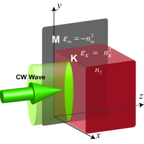
Figure 2: Parallel illumination of a metal/Kerr interface from the Kerr medium.

VI.2 Coupling of a nonlinear plasmon and a soliton in a MK structure

We analyze now another interesting case, namely, that of a metal surface directly attached to the Kerr medium and subject to parallel illumination by means of a spatial soliton of the Kerr medium (see Fig.2). In this situation, the dielectric slab of the MDK structure analyzed in the previous section is no longer present. This has two important consequences in the mathematical description of the problem: firstly, the linear index contrast between the dielectric and Kerr medium of the MDK structure disappears, $\varepsilon_{d}=\varepsilon_{\mathrm{K}}$; and, secondly, because the Kerr medium is now attached to the metal, Kerr nonlinearities directly affect the SPP, so that it is required to consider a nonlinear plasmon instead of its linear counterpart. Let us see how these two features affect the soliplasmon propagation equation.

As before, we work at leading order of the weak coupling approximation, so Eq.(45) is the correct variational propagation equation to use in this case. The first consequence of working with a MK structure instead of with a MDK one is that the plasmon-to-soliton coupling completely disappears. Indeed, according to Eq.(31) $\Delta\varepsilon_{p}=0$ and, therefore, $\triangle_{sp}=0$ according to the definition (41). On the other hand, the plasmon propagation constant $\mathrm{\beta{}_{np}}$ is now that of a stationary nonlinear plasmon and it depends on the SPP amplitude $|A|$. The analytic form of $\beta_{\mathrm{np}}$ on $|A|$ is know only in some cases Agranovich_JETP_1980 . In the general case, $\beta_{\mathrm{np}}^{2}$ is nothing but the eigenvalue of the nonlinear equation for the electric components of the nonlinear SPP field (18). As explained in Section IV, the nonlinear terms in this equation depend nonlinearly on the plasmon amplitude as $|A|^{2}$ . So that, $\beta_{\mathrm{np}}^{2}=\beta_{\mathrm{np}}^{2}(|A|^{2})$ and we can always perform a Taylor expansion in $|A|^{2}$:

$$\beta_{\mathrm{np}}^{2}=\beta_{\mathrm{p}}^{2}+k_{0}^{2}\gamma_{p}|A|^{2}+O(|A|^{4}).$$

We are interested here in the first order nonlinear corrections to the linear case, so that we keep the first correction only and neglect $O(|A|^{4})$ terms. Consequently, to leading order in the weak coupling approximation and to first order in $|A|^{2}$, we have

$$\left(\frac{d^{2}}{dz^{2}}+\beta_{\mathrm{np}}^{2}\right)A =- \frac{\Delta_{ps}}{N_{\mathrm{np}}}C-\frac{\Delta_{\mathrm{K}}}{N_{\mathrm{np}}}\left(2|A|^{2}C+A^{2}C^{*}\right)$$

$$\left(\frac{d^{2}}{dz^{2}}+\beta_{s}^{2}\right)C = 0.$$ (53)

We can write the previous equation in a form that resemble that of a linear plasmon in Eq.(46).

$$\left[\frac{d^{2}}{dz^{2}}+\bar{\beta}_{np}^{2}\left(A,C\right)\right]A =- \frac{\bar{\Delta}_{ps}\left(|A|,|C|\right)}{N_{\mathrm{np}}}C$$

$$\left[\frac{d^{2}}{dz^{2}}+\beta_{s}^{2}\left(|C|\right)\right]C = 0,$$ (54)

where now

$$\bar{\beta}_{np}^{2}\left(A,C\right) = \beta_{\mathrm{p}}^{2}+k_{0}^{2}\gamma_{p}|A|^{2}+\frac{\Delta_{\mathrm{K}}\left(|C|\right)}{N_{\mathrm{np}}}AC^{*}$$

$$\bar{\Delta}_{ps}\left(|A|,|C|\right) = \Delta_{ps}(|C|)+2\Delta_{\mathrm{K}}(|C|)|A|^{2}.$$ (55)

Note that the effective propagation constant is now a complex number $\bar{\beta}_{\mathrm{np}}\in\mathbb{C}$ because of the nonlinear $AC^{*}$ coupling. Thus the nonlinear soliton-to-plasmon coupling simultaneously affects both the phase velocity of the nonlinear plasmon and the plasmon amplitude, due to the presence of a nonzero gain-loss coefficient proportional to the imaginary part of the effective propagation constant: $\Im(\bar{\beta}_{\mathrm{np}}^{2})\sim\sin\left(\varphi_{p}-\varphi_{s}\right)\neq 0,$ in general. There is also a nonlinear plasmonic modification of the coupling coefficient $\Delta_{ps}$ in Eq.(55) that can slightly modify the nature of the coupling with respect the pure MDK case. These two effects are additional to those associated to the $A$-independent coefficient $\Delta_{ps}(|C|)$ appearing in the case of the linear-plasmon/soliton coupling in a MDK structure Milian_OL_2012 .

We see that, at this order of the weak coupling approximation, the soliton equation decouples from the plasmon one. Physically speaking, the soliton acts as a non-depleting reservoir pumping the non-linear plasmon without experience any energy exchange with the SPP. Obviously, this is only true within the order of our approximation because we have truncated higher-order terms. Indeed, there exists this type of energy exchange from the plasmon to the soliton but this has to fulfill two conditions: (i), it has to be very small, i.e., in mathematical terms is has to be at least $O(e^{-\kappa_{s}a})^{2}$ since this is the order of terms neglected in our weak coupling approximation; and (ii), it necessarily has to arise from terms neglected in the process of deriving the variational equations at leading order, since the leading order plasmon-to-soliton coupling for a MK structure, linked to variations in the linear dielectric functions, is strictly zero inasmuch $\triangle\varepsilon_{p}=0$. So, we would need to go to next-to-leading order in the weak coupling approximation if we wanted to account for these effects.

This generalization to next-to-leading order is certainly more complicated because we need to include terms that we have neglected in previous analysis. If we keep all the approximations to the same order, as before, and we only go to the next order in the weak coupling approximation, we need to consider the four terms in the Kerr coupling $Q_{\mathrm{K}}$ defined in Eq.(35) . We have to retained now the first two terms. We neglected them before because they provided terms $O(e^{-\kappa_{s}a})^{2}$ that we want to keep now. The plasmon and soliton projections provide two more terms linked to them. The plasmonic projection (37) is now:

$$N_{\mathrm{np}}\left[\frac{d^{2}}{dz^{2}}A+\beta_{\mathrm{np}}^{2}A\right]+\delta_{ps}\left[\frac{d^{2}}{dz^{2}}C+\beta_{\mathrm{s}}^{2}C\right] = -\triangle_{pp}A-\triangle_{ps}C$$

$$-\triangle_{\mathrm{K}}\left[2|A|^{2}C+A^{2}C^{*}\right]-\Gamma_{\mathrm{K}}\left[2|C|^{2}A+C^{2}A^{*}\right],$$

whereas the soliton projection reads (40)

$$\delta_{sp}\left[\frac{d^{2}}{dz^{2}}A+\beta_{\mathrm{np}}^{2}A\right]+N_{s}\left[\frac{d^{2}}{dz^{2}}C+\beta_{\mathrm{s}}^{2}C\right] = -\triangle_{ss}C-\triangle_{sp}A$$

$$-\triangle^{\prime}_{\mathrm{K}}\left[2|A|^{2}C+A^{2}C^{*}\right]-\Gamma^{\prime}_{\mathrm{K}}\left[2|C|^{2}A+C^{2}A^{*}\right],$$

where we have introduced two new Kerr coupling coefficients:

$$\Gamma_{\mathrm{K}} \equiv k_{0}^{2}\int_{\mathbb{R}}\gamma f_{\mathrm{np}}(0)f_{\mathrm{np}}(z)f_{s}^{2}(z)$$

$$\Gamma^{\prime}_{\mathrm{K}} \equiv k_{0}^{2}\int_{\mathbb{R}}\gamma f_{s}(0)f_{\mathrm{np}}(z)f_{s}^{2}(z).$$

However, since $\triangle\varepsilon_{p}=0$, we know that their two projections vanish, so that, $\Delta_{sp}=0$ and $\Delta_{pp}=0$. If we follow now the demonstration given in Section V, we can conclude that the form of the generalized equation (43) has to be substituted by a new one including the new Kerr-coupling terms and in which $q_{sp}=0$ (from its definition Eq.(44) along with $\Delta_{sp}=0$ and $\Delta_{pp}=0$):

$$\left(\frac{d^{2}}{dz^{2}}+B_{\mathrm{np}}^{2}\right)A = -q_{ps}C-q_{\mathrm{K}}\left(2|A|^{2}C+A^{2}C^{*}\right)-p_{\mathrm{K}}\left(2|C|^{2}A+C^{2}A^{*}\right)$$

$$\left(\frac{d^{2}}{dz^{2}}+B_{s}^{2}\right)C = -q^{\prime}_{\mathrm{K}}\left(2|A|^{2}C+A^{2}C^{*}\right)-p^{\prime}_{\mathrm{K}}\left(2|C|^{2}A+C^{2}A^{*}\right),$$ (56)

where we have introduced the new nonlinear coefficients

$$p{}_{K} = \frac{N_{s}\Gamma{}_{\mathrm{K}}-\delta_{ps}\Gamma^{\prime}_{\mathrm{K}}}{N_{\mathrm{np}}N_{s}-\text{$\delta$}_{ps}\delta_{sp}}$$

$$p^{\prime}_{K} = \frac{N_{\mathrm{np}}\Gamma^{\prime}_{\mathrm{K}}-\delta_{sp}\Gamma_{\mathrm{K}}}{N_{\mathrm{np}}N_{s}-\text{$\delta$}_{ps}\delta_{sp}}.$$ (57)

We see that, as expected, despite there is no trace of linear plasmon-to-soliton coupling, nonlinear coupling occurs in the next-to-leading order weak coupling approximation. It is revealing to consider the case of a very weak plasmon field, in which we are approaching the linear plasmon limit and thus terms $O(A^{2})$ can be neglected in Eq.(56):

$$\left(\frac{d^{2}}{dz^{2}}+B_{\mathrm{np}}^{2}\right)A = -q_{ps}C-p_{\mathrm{K}}\left(2|C|^{2}A+C^{2}A^{*}\right)$$

$$\left(\frac{d^{2}}{dz^{2}}+B_{s}^{2}\right)C = -p^{\prime}_{\mathrm{K}}\left(2|C|^{2}A+C^{2}A^{*}\right).$$ (58)

The previous equation makes clear that there is a second mechanism for plasmon-to-soliton coupling absent at leading order. Soliton can be also pumped or depleted by the plasmon field through a mechanism based on the Kerr coupling terms in Eq.(58). These terms can be understood as nonlinear sources generating gain or loss on the soliton parameter $C$ and driven by the plasmon field. As before, this mechanism can be visualized by renormalizing the soliton propagation constant in the following way:

$$\bar{B}_{s}^{2}\equiv B_{s}^{2}+p^{\prime}_{\mathrm{K}}\left(2C^{*}A+CA^{*}\right),$$

which permits to write the soliton equation as:

$$\left(\frac{d^{2}}{dz^{2}}+\bar{B}_{s}^{2}\right)C=0.$$

Analogously as in a previous analysis, the imaginary part of the renormalized propagation constant give us essential information about this nonlinear mechanism

$$\Im(\bar{B}_{s}^{2})=p^{\prime}_{\mathrm{K}}|C||A|\sin\left(\varphi_{p}-\varphi_{s}\right),$$

which indicates that this type of term generates nonlinear gain or loss depending on the value of the soliplasmon relative phase.

Another way of understanding the physical nature of the plasmon-to-soliton nonlinear term (the one proportional to $p^{\prime}_{\mathrm{K}}$) in Eq.(58), and more specifically the one depending on $|C|^{2}$, is by considering that its origin is the nonlinear modulation of the dielectric function in the Kerr medium. We know that the absence of linear modulation ($\triangle\varepsilon_{p}=0$) makes the plasmon-to-soliton linear coupling to vanish. However, even if there is no linear modulation in the region where the soliton is localized (we assume an homogeneous nonlinear dielectric medium), the Kerr effect does induce a nonlinear modulation of the refractive index or, equivalently, of the dielectric function $\varepsilon(x)=\varepsilon_{\mathrm{K}}+\gamma|E_{s}(x)|^{2}$. Therefore, there exists, in fact, an effective modulation of $\varepsilon(x)$ induced by the Kerr nonlinearity that, in turn, originates a local variation of the dielectric function for the plasmon field, as defined in Eq.(31), given by

$$\triangle\varepsilon_{p}^{\mathrm{NL}}(x)=\varepsilon(x)-\varepsilon_{p}(x)=\varepsilon(x)-\varepsilon_{\mathrm{K}}=\gamma|E_{s}|^{2}\,\,\,\mathrm{if}\,\,\,x>0.$$

Since this term is nonzero, an effective plasmon-to-soliton variational coupling, analogous to the linear one $\Delta_{sp}$ (Eq.(41)), is expected (recall that the linear coefficient vanish, $\Delta_{sp}=0$)

$$\triangle_{sp}^{\mathrm{NL}}\equiv k_{0}^{2}\int_{\mathbb{R}}f_{s}(0)\triangle\varepsilon_{p}^{\mathrm{NL}}f_{\mathrm{np}}(z)=k_{0}^{2}|C|^{2}\int_{\mathbb{R}}\gamma f_{s}(0)f_{s}^{2}(z)f_{\mathrm{np}}(z)=\Gamma^{\prime}_{\mathrm{K}}|C|^{2}.$$

The previous variational term corresponds to the soliton projection of $\triangle\varepsilon_{p}^{\mathrm{NL}}$. One recognizes that this term is responsible of the first term of the $p^{\prime}_{\mathrm{K}}$ coefficient in Eq.(57). This term can be interpreted as the leading order effect of soliton-soliton interaction in the weak coupling regime. In this case, the nonlinear plasmon, acting as a soliton, couples to the soliton tail though its own asymptotic exponential tail by means of the Kerr term. The soliton-soliton interaction exists independently of the existence of a linear modulation and, therefore, occurs even in a completely homogeneous medium. For this reason, it is expected to exist even if the soliton moves in a completely homogeneous medium, as in the present case in which we deal with a MK structure. Analogously, the nonlinear self-modulated local variation of the dielectric function $\triangle\varepsilon_{p}^{\mathrm{NL}}$ generates also a next-to-leading order coupling through its plasmon projection, which physically can be interpreted as generated by a nonlinearly induced term $\Delta_{pp}^{\mathrm{NL}}$ of the type given in Eq.(39) (recall that there is no linear counterpart of this term since $\Delta_{pp}=0$):

$$\triangle_{pp}^{\mathrm{NL}}\equiv k_{0}^{2}\int_{\mathbb{R}}f_{\mathrm{np}}(0)\triangle\varepsilon_{p}^{\mathrm{NL}}f_{\mathrm{np}}(z)=k_{0}^{2}|C|^{2}\int_{\mathbb{R}}\gamma f_{\mathrm{np}}(0)f_{s}^{2}(z)f_{\mathrm{np}}(z)=\Gamma{}_{\mathrm{K}}|C|^{2}.$$

This coupling coefficient generates the second term in the expression for $p^{\prime}_{\mathrm{K}}$ (39).

VII Conclusions

We have introduced a variational approach to properly understand the physics behind the problem of the nonlinear excitation of a SPP by a spatial soliton. Unlike in the original proposal in Ref.Bliokh_PRA_2009 , the resulting nonlinear resonator model is obtained from first principles, which permits, in this way, to provide an approximate solution of the full vector Maxwell’s wave equation (1) for configurations close to our soliplasmon ansatz (27). In physical terms, variational equations extract the most relevant information of soliplasmon resonances as bound states of a soliton and a linear or nonlinear SPP. They provide the dynamics of a SPP and a soliton propagating along a metal/dielectric interface in the presence of a continuous exchange of electromagnetic energy between them in a process controlled by a nonlinear coupling constant, which is proportional to the soliton field at the interface $e^{-\kappa_{s}a}$ (see Eq.(VI.1)). Since the inverse soliton penetration length $\kappa_{s}=\left(\gamma/2\right)^{1/2}k_{0}|C(z)|$ depends nonlinearly on the soliton amplitude, even the simpler case of a soliton bounded to a linear SPP presents special features with respect other well-know nonlinear resonator models Eks_PRA_2011 .

On the other hand, the fact that soliplasmon resonances exists even in the presence of a low power SPP component, i.e, a linear SPP, demonstrates that nonlinearities in a soliplasmon play also a supplementary role than the one that is commonly attributed to them in nonlinear plasmonics. The fact that SPP’s can support very high intensities very close to the metal/nonlinear-dielectric interface is the origin of most of the nonlinear effects reported in the literature. They are responsible of generation of second harmonic (see, e.g., Zayats_PR_2005 and references therein) but also of nonlinearities of the Kerr type. They are known as early as in the 80’s Agranovich_JETP_1980 ; Tomlinson_OL_1980 ; Akhmediev_JETP_1982 ; Yu1983a ; Leung_PRB_1985 ; Mihalache_PS_1984 ; Stegeman1985a ; Ariyasu_JAP_1985 . More recently, substantial advances in the field of plasmonics have refreshed the possibility of exploiting these effects for nanophotonics applications using available technology, so a renovated interest in nonlinear effects induced by Kerr materials interacting with metals have been reflected in the literature (see, for example, Feigenbaum_OL_2007 ; Davoyan_OE_2009 ; Ye_PRL_2010 ; Salgueiro_APL_2010 ; Skryabin_JOSAB_2011 ; Marini_OE_2011 ; Marini_PRA_2011 ; Milian_APL_2011 ; Noskov_PRL_2012 ). The high intensities reached in the dielectric in the vicinity of the metal interface associated to a high-power SPP mode are able to enhance the nonlinear response of a Kerr medium directly attached to the metal. This response can, in return, modify the propagation properties of the SPP. As pointed out as early as in Ref.Stegeman1985a , "when nonlinear dielectric media are in contact with a metal surface, the surface plasmon polaritons guided by that interface become power-dependent." This can be considered a standard definition of a nonlinear plasmon. The fact that the propagation constant of the SPP becomes power-dependent explicitly shows that, according to this definition of a nonlinear plasmon, the latter is continuously connected to the linear SPP in a standard $P$ vs $\mu$ representation. From this perspective, soliplasmons are not nonlinear plasmons since their resonant nature forces their two branches —corresponding to 0- and $\pi$- soliplasmon solutions— to be detached from that of a linear SPP in a $P$ vs $\mu$ representation (see its resonant behavior in Ref.Milian_OL_2012 ). Physically, in a soliplasmon, plasmon and soliton preserve their identity as localized solutions even though they are interacting. In a nonlinear plasmon, the soliton cannot be resolved as a second spatially localized component. Our variational approach for a soliplasmon formalizes this features explicitly by assuming the existence of two separately localized plasmon and soliton components in our ansatz (2). In this way, our variational equations distinguish between two different types of nonlinear effects: (i) those affecting the uncoupled propagation of the plasmon and soliton components, i.e, those which appear even when they do not interact; and (ii) those related to the interaction. In the case of the SPP, the former are taken into account in our variational formalism through the dependence of the plasmon propagation constant $\beta_{\mathrm{np}}^{2}=\beta_{\mathrm{np}}^{2}(|A|^{2})$ on the SPP amplitude. This is analogous to the well-known behavior of the soliton propagation constant with respect to its amplitude: $\beta_{s}^{2}=\beta_{s}^{2}(|C|^{2})$. The second type of nonlinear effects are related to coupling. Here we can, in turn, distinguish two different categories. The first one is related to typical soliton-to-soliton coupling, as those appearing in Eqs.(53) or (58), which show a form analogous to cross-phase modulation Kivshar_book_2006 . The second one is related to the modulation of the linear dielectric function and it is the analogous to the coupling between neighboring atoms in a crystal in the so-called tight binding approximation Ashcroft_book_1976 . The coupling here is giving by the overlapping of the wave functions of two solutions of individual atomic sites detached from one another weighted by the difference of the total periodic potential with respect the atomic one. This is the nature of the coupling terms $\Delta_{sp}$ and $\Delta_{ps}$ involving the local variations of the linear dielectric function $\triangle\varepsilon_{p}$ and $\triangle\varepsilon_{s}$ in Eqs.(38) and (41). This is in fact the dominant coupling term in the weak coupling approximation, as demonstrated by our variational equations for the interaction of a linear plasmon and a soliton (46). However, since the overlapping solutions are in this case nonlinear (in this case, that of the the soliton), the coupling becomes itself nonlinear. It is precisely this second type of nonlinearity in the coupling what causes the soliplasmon variational model to be qualitatively different from other coupled nonlinear systems Eks_PRA_2011 .

The work of A. F. was partially supported by the MINECO under the TEC2010-15327 grant.

References

• (1) K. Y. Bliokh, Y. P. Bliokh, and A. Ferrando, Phys. Rev. A 79, 041803 (2009).
• (2) C. Milián, D. E. Ceballos-Herrera, D. V. Skryabin, and A. Ferrando, Opt. Lett. 37, 4221 (2012).
• (3) V. M. Agranovich, V. S. Babichenko, and V. Ya. Chernyak, Sov. Phys. JETP Lett. 32, 512 (1980).
• (4) W. J. Tomlinson, Opt. Lett. 5, 323 (1980).
• (5) N. N. Akhmediev, Sov. Phys. JETP 56, 299 (1982).
• (6) M. Yu, Phys. Rev. A 28, 1855 (1983).
• (7) K. M. Leung, Phys. Rev. B 32, 5093 (1985).
• (8) D. Mihalache, R. G. Nazmitdinov, and V. K. Fedyanin, Phys. Scripta 29, 269 (1984).
• (9) G. I. Stegeman, C. T. Seaton, J. Ariyasu, R. F. Wallis, and A. A. Maradudin J. Appl. Phys. 58, 2453 (1985).
• (10) J. Ariyasu, C. T. Seaton, G. I. Stegeman, A. A. Maradudin, and R. F. Wallis, J. Appl. Phys. 58, 2460 (1985).
• (11) W. Walasik, V. Nazabal, M. Chauvet, Y. Kartashov, and G. Renversez, Opt. Lett. 37, 4579 (2012).
• (12) A. Ciattoni, B. Crosignani, P. Di Porto, and A. Yariv, J. Opt. Soc. Am. B 22, 1384 (2005).
• (13) A. W. Snyder and J. D. Love, Optical waveguide theory, (Chapman and Hall, London; New York, 1983).
• (14) N. W. Ashcroft and N. D. Mermin, Solid state physics, (Saunders College Publishing, 1976).
• (15) S. A. Maier, Plasmonics: Fundamentals and Applications (Springer, New York, 2007).
• (16) J. M. Pitarke, V. M. Silkin, E. V. Chulkov, and P. M. Echenique, Rep. Prog. Phys. 70, 1 (2007).
• (17) Y. Ekşioğlu, O. E. Müstecaplioğlu, and K. Güven, Phys. Rev. A 84, 033805 (2011).
• (18) A. V. Zayats, I. I. Smolyaninov, and A. A. Maradudin, Phys. Rep. 408, 131 (2005).
• (19) Y. S. Kivshar and G. P. Agrawal, Optical Solitons. From Fibers to Photonic Crystals (Academic Press, San Diego, 2003).
• (20) E. Feigenbaum and M. Orenstein, Opt. Lett. 32, 674 (2007).
• (21) A. R. Davoyan, I. V. Shadrivov, and Y. S. Kivshar, Opt. Express 17, 21732 (2009).
• (22) F. Ye, D. Mihalache, B. Hu, and N. C. Panoiu, Phys. Rev. Lett. 104, 106802 (2010).
• (23) J. R. Salgueiro and Y. S. Kivshar, Appl. Phys. Lett. 97, 081106 (2010).
• (24) D. V. Skryabin, A. V. Gorbach, and A. Marini, J. Opt. Soc. Am. B 28, 109 (2011).
• (25) A. Marini, D. V. Skryabin, and B. Malomed, Opt. Express 19, 6616 (2011).
• (26) A. Marini and D. V. Skryabin, Phys. Rev. A 81, 033850 (2010).
• (27) C. Milián and D. V. Skryabin, Appl. Phys. Lett. 98, 111104 (2011).
• (28) R. E. Noskov, P. A. Belov, and Y. S. Kivshar, Phys. Rev. Lett. 108, 093901 (2012).