Model Reduction of Descriptor Systems by Interpolatory Projection Methods

Abstract

In this paper, we investigate interpolatory projection framework for model reduction of descriptor systems. With a simple numerical example, we first illustrate that employing subspace conditions from the standard state space settings to descriptor systems generically leads to unbounded ${{\mathcal{H}}_{2}}$ or ${{\mathcal{H}}_{\infty}}$ errors due to the mismatch of the polynomial parts of the full and reduced-order transfer functions. We then develop modified interpolatory subspace conditions based on the deflating subspaces that guarantee a bounded error. For the special cases of index-$1$ and index-$2$ descriptor systems, we also show how to avoid computing these deflating subspaces explicitly while still enforcing interpolation. The question of how to choose interpolation points optimally naturally arises as in the standard state space setting. We answer this question in the framework of the ${{\mathcal{H}}_{2}}$-norm by extending the Iterative Rational Krylov Algorithm (IRKA) to descriptor systems. Several numerical examples are used to illustrate the theoretical discussion.

1 Introduction

We discuss interpolatory model reduction of differential-algebraic equations (DAEs), or descriptor systems, given by

$$\begin{array}[]{rcl}{\mathbf{E}}\,\dot{{\mathbf{x}}}(t)&=&{\mathbf{A}}{\mathbf{x}}(t)+{\mathbf{B}}{\mathbf{u}}(t),\\ {\mathbf{y}}(t)&=&{\mathbf{C}}{\mathbf{x}}(t)+{\mathbf{D}}{\mathbf{u}}(t),\end{array}$$ (1)

where ${\mathbf{x}}(t)\in\mbox{\Bb R}^{n}$, ${\mathbf{u}}(t)\in\mbox{\Bb R}^{m}$ and ${\mathbf{y}}(t)\in\mbox{\Bb R}^{p}$ are the states, inputs and outputs, respectively, ${\mathbf{E}}\in\mbox{\Bb R}^{n\times n}$ is a singular matrix, ${\mathbf{A}}\in\mbox{\Bb R}^{n\times n}$, ${\mathbf{B}}\in\mbox{\Bb R}^{n\times m}$, ${\mathbf{C}}\in\mbox{\Bb R}^{p\times n}$, and ${\mathbf{D}}\in\mbox{\Bb R}^{p\times m}$. Taking the Laplace transformation of system (1) with zero initial condition ${\mathbf{x}}(0)=\mathbf{0}$, we obtain $\widehat{{\mathbf{y}}}(s)={\mathbf{G}}(s)\widehat{{\mathbf{u}}}(s)$, where $\widehat{{\mathbf{u}}}(s)$ and $\widehat{{\mathbf{y}}}(s)$ denote the Laplace transforms of ${\mathbf{u}}(t)$ and ${\mathbf{y}}(t)$, respectively, and ${\mathbf{G}}(s)={\mathbf{C}}(s{\mathbf{E}}-{\mathbf{A}})^{-1}{\mathbf{B}}+{\mathbf{D}}$ is a transfer function of (1). By following the standard abuse of notation, we will denote both the dynamical system and its transfer function by ${\mathbf{G}}$.

Systems of the form (1) with extremely large state space dimension $n$ arise in various applications such as electrical circuit simulations, multibody dynamics, or semidiscretized partial differential equations. Simulation and control in these large-scale settings is a huge computational burden. Efficient model utilization becomes crucial where model reduction offers a remedy. The goal of model reduction is to replace the original dynamics in (1) by a model of the same form but with much smaller state space dimension such that this reduced model is a high fidelity approximation to the original one. Hence, we seek a reduced-order model

$$\begin{array}[]{rcl}{\widetilde{{\mathbf{E}}}}\,\dot{\widetilde{{\mathbf{x}}}}(t)&=&{\widetilde{{\mathbf{A}}}}\widetilde{{\mathbf{x}}}(t)+{\widetilde{{\mathbf{B}}}}{\mathbf{u}}(t),\\ \widetilde{{\mathbf{y}}}(t)&=&{\widetilde{{\mathbf{C}}}}\widetilde{{\mathbf{x}}}(t)+{\widetilde{{\mathbf{D}}}}{\mathbf{u}}(t),\end{array}$$ (2)

where ${\widetilde{{\mathbf{E}}}},{\widetilde{{\mathbf{A}}}}\in\mbox{\Bb R}^{r\times r}$, ${\widetilde{{\mathbf{B}}}}\in\mbox{\Bb R}^{r\times m}$, ${\widetilde{{\mathbf{C}}}}\in\mbox{\Bb R}^{p\times r}$, and ${\widetilde{{\mathbf{D}}}}\in\mbox{\Bb R}^{p\times m}$ such that $r\ll n$, and the error ${\mathbf{y}}-\widetilde{{\mathbf{y}}}$ is small with respect to a specific norm over a wide range of inputs ${\mathbf{u}}(t)$ with bounded energy. In the frequency domain, this means that the transfer function of (2) given by ${\widetilde{{\mathbf{G}}}}(s)={\widetilde{{\mathbf{C}}}}(s{\widetilde{{\mathbf{E}}}}-{\widetilde{{\mathbf{A}}}})^{-1}{\widetilde{{\mathbf{B}}}}+{\widetilde{{\mathbf{D}}}}$ approximates ${\mathbf{G}}(s)$ well, i.e., the error ${\mathbf{G}}(s)-{\widetilde{{\mathbf{G}}}}(s)$ is small in a certain system norm.

The reduced-order model (2) can be obtained via projection as follows. We first construct two $n\times r$ matrices ${\mathbf{V}}$ and ${\mathbf{W}}$, approximate the full-order state ${\mathbf{x}}(t)$ by ${\mathbf{V}}\widetilde{{\mathbf{x}}}(t)$, and then enforce the Petrov-Galerkin condition

$$\mathbf{W}^{T}\left({\mathbf{E}}{\mathbf{V}}\dot{\widetilde{{\mathbf{x}}}}(t)-{\mathbf{A}}{\mathbf{V}}\widetilde{{\mathbf{x}}}(t)-{\mathbf{B}}\,{\mathbf{u}}(t)\right)=\mathbf{0},\qquad\quad\widetilde{{\mathbf{y}}}(t)={\mathbf{C}}{\mathbf{V}}\widetilde{{\mathbf{x}}}(t)+{\mathbf{D}}{\mathbf{u}}(t).$$

As a result, we obtain the reduced-order model (2) with the system matrices

$$\begin{array}[]{ll}{\widetilde{{\mathbf{E}}}}={\mathbf{W}}^{T}{\mathbf{E}}{\mathbf{V}},&\qquad{\widetilde{{\mathbf{A}}}}={\mathbf{W}}^{T}{\mathbf{A}}{\mathbf{V}},\\[7.22743pt] {\widetilde{{\mathbf{B}}}}={\mathbf{W}}^{T}{\mathbf{B}},&\qquad{\widetilde{{\mathbf{C}}}}={\mathbf{C}}{\mathbf{V}},\qquad{\widetilde{{\mathbf{D}}}}={\mathbf{D}}.\end{array}$$ (3)

The projection matrices ${\mathbf{V}}$ and ${\mathbf{W}}$ determine the subspaces of interest and can be computed in many different ways.

In this paper, we consider projection-based interpolatory model reduction methods, where the choice of ${\mathbf{V}}$ and ${\mathbf{W}}$ enforces certain tangential interpolation of the original transfer function. These methods will be presented in Section 2 in more detail. Projection-based interpolation with multiple interpolation points was initially proposed by Skelton et. al. in [7, 31, 32]. Grimme [10] has later developed a numerically efficient framework using the rational Krylov subspace method of Ruhe [24]. The tangential rational interpolation framework, we will be using here, is due to a recent work by Gallivan et al. [9].

Unfortunately, it is often assumed that extending interpolatory model reduction from standard state space systems with ${\mathbf{E}}={\mathbf{I}}$ to descriptor systems with singular ${\mathbf{E}}$ is as simple as replacing ${\mathbf{I}}$ by ${\mathbf{E}}$. In Section 2, we present an example showing that this naive approach may lead to a poor approximation with an unbounded error ${\mathbf{G}}(s)-{\widetilde{{\mathbf{G}}}}(s)$ although the classical interpolatory subspace conditions are satisfied. In Section 3, we modify these conditions in order to enforce bounded error. The theoretical result will take advantage of the spectral projectors. Then using the new subspace conditions, we extend in Section 4 the optimal ${{\mathcal{H}}_{2}}$ model reduction method of [15] to descriptor systems. Sections 3 and 4 make explicit usage of deflating subspaces which could be numerically demanding for general problems. Thus, for the special cases of index-1 and index-2 descriptor systems, we show in Sections 5 and 6, respectively, how to apply interpolatory model reduction without explicitly computing the deflating subspaces. Theoretical discussion will be supported by several numerical examples. In particular, in Section 5.2, we present an example, where the balanced truncation approach [26] is prone to failing due to problems solving the generalized Lyapunov equations, while the (optimal) interpolatory model reduction can be effectively applied.

2 Model reduction by tangential rational interpolation

The goal of model reduction by tangential interpolation is to construct a reduced-order model (2) such that its transfer function ${\widetilde{{\mathbf{G}}}}(s)$ interpolates the original one, ${\mathbf{G}}(s)$, at selected points in the complex plane along selected directions. We will use the notation of [1] to define this problem more precisely: Given ${\mathbf{G}}(s)={\mathbf{C}}(s{\mathbf{E}}-{\mathbf{A}})^{-1}{\mathbf{B}}+{\mathbf{D}}$, the left interpolation points $\{\mu_{i}\}_{i=1}^{q}$, $\mu_{i}\in\mbox{\Bb C}$, together with the left tangential directions $\{\mathbf{\mathsf{c}}_{i}\}_{i=1}^{q}$, $\mathbf{\mathsf{c}}_{i}\in\mbox{\Bb C}^{p}$, and the right interpolation points $\{\sigma_{j}\}_{j=1}^{r}$, $\sigma_{j}\in\mbox{\Bb C}$, together with the right tangential directions $\{\mathbf{\mathsf{b}}_{j}\}_{j=1}^{r}$, $\mathbf{\mathsf{b}}_{j}\in\mbox{\Bb C}^{m}$, we seek to find a reduced-order model ${\widetilde{{\mathbf{G}}}}(s)={\widetilde{{\mathbf{C}}}}(s{\widetilde{{\mathbf{E}}}}-{\widetilde{{\mathbf{A}}}})^{-1}{\widetilde{{\mathbf{B}}}}+{\widetilde{{\mathbf{D}}}}$ that is a tangential interpolant to ${\mathbf{G}}(s)$, i.e.,

$$\begin{array}[]{ll}\mathbf{\mathsf{c}}_{i}^{T}{\mathbf{G}}(\mu_{i})=\mathbf{\mathsf{c}}_{i}^{T}{\widetilde{{\mathbf{G}}}}(\mu_{i}),&\quad i=1,\ldots,q,\\[5.69054pt] {\mathbf{G}}(\sigma_{j})\mathbf{\mathsf{b}}_{j}={\widetilde{{\mathbf{G}}}}(\sigma_{j})\mathbf{\mathsf{b}}_{j},&\quad j=1,\ldots,r.\end{array}$$ (4)

Through out the paper, we will assume $q=r$, meaning that the same number of left and right interpolation points are used. In addition to interpolating ${\mathbf{G}}(s)$, one might ask for matching the higher-order derivatives of ${\mathbf{G}}(s)$ along the tangential directions as well. This scenario will also be handled.

By combining the projection-based reduced-order modeling technique with the interpolation framework, we want to find the $n\times r$ matrices ${\mathbf{W}}$ and ${\mathbf{V}}$ such that the reduced-order model (2), (3) satisfies the tangential interpolation conditions (4). This approach is called projection-based interpolatory model reduction. How to enforce the interpolation conditions via projection is shown in the following theorem, where the $\ell$-th derivative of ${\mathbf{G}}(s)$ with respect to $s$ evaluated at $s=\sigma$ is denoted by ${\mathbf{G}}^{(\ell)}(\sigma)$.

Theorem 1.

[1, 9] Let $\sigma,\,\mu\in\mbox{\Bb C}$ be such that $s\,{\mathbf{E}}-{\mathbf{A}}$ and $s\,{\widetilde{{\mathbf{E}}}}-{\widetilde{{\mathbf{A}}}}$ are both invertible for $s=\sigma,\,\mu$, and let $\mathbf{\mathsf{b}}\in\mbox{\Bb C}^{m}$ and $\mathbf{\mathsf{c}}\in\mbox{\Bb C}^{p}$ be fixed nontrivial vectors.

1. If

   $$\bigl{(}\left(\sigma\,{\mathbf{E}}-{\mathbf{A}}\right)^{-1}{\mathbf{E}}\bigr{)}^{j-1}\left(\sigma\,{\mathbf{E}}-{\mathbf{A}}\right)^{-1}{\mathbf{B}}\mathbf{\mathsf{b}}\in\mbox{{Im}}({\mathbf{V}}),\enskip j=1,\ldots,N,$$ (5)

   then ${\mathbf{G}}^{(\ell)}(\sigma)\mathbf{\mathsf{b}}={\widetilde{{\mathbf{G}}}}^{(\ell)}(\sigma)\mathbf{\mathsf{b}}$ for $\ell=0,1,\ldots,N-1$.

2. If

   $$\bigl{(}\left(\mu\,{\mathbf{E}}-{\mathbf{A}}\right)^{-T}{\mathbf{E}}^{T}\bigr{)}^{j-1}\left(\mu\,{\mathbf{E}}-{\mathbf{A}}\right)^{-T}{\mathbf{C}}^{T}\mathbf{\mathsf{c}}\in\mbox{{Im}}({\mathbf{W}}),\enskip j=1,\ldots,M,$$ (6)

   then $\mathbf{\mathsf{c}}^{T}{\mathbf{G}}^{(\ell)}(\mu)=\mathbf{\mathsf{c}}^{T}{\widetilde{{\mathbf{G}}}}^{(\ell)}(\mu)$ for $\ell=0,1,\ldots,M-1$.

3. If both (5) and (6) hold, and if $\sigma=\mu$, then $\mathbf{\mathsf{c}}^{T}{\mathbf{G}}^{(\ell)}(\sigma)\mathbf{\mathsf{b}}=\mathbf{\mathsf{c}}^{T}{\widetilde{{\mathbf{G}}}}^{(\ell)}(\sigma)\mathbf{\mathsf{b}}$ for $\ell=0,1,\ldots,M+N+1$.

One can see that to solve the rational tangential interpolation problem via projection all one has to do is to construct the matrices ${\mathbf{V}}$ and ${\mathbf{W}}$ as in Theorem 1. The dominant cost is to solve sparse linear systems. We also note that in Theorem 1 the values that are interpolated are never explicitly computed. This is crucial since that computation is known to be poorly conditioned [8].

To illustrate the result of Theorem 1 for a special case of Hermite bi-tangential interpolation, we take the same right and left interpolation points $\{\sigma_{i}\}_{i=1}^{r}$, left tangential directions $\{\mathbf{\mathsf{c}}_{i}\}_{i=1}^{r}$, and right tangential directions $\{\mathbf{\mathsf{b}}_{i}\}_{i=1}^{r}$. Then for the projection matrices

$${\mathbf{V}} = \left[(\sigma_{1}{\mathbf{E}}-{\mathbf{A}})^{-1}{\mathbf{B}}\mathbf{\mathsf{b}}_{1},\;\,~{}\cdots,~{}\;\,(\sigma_{r}{\mathbf{E}}-{\mathbf{A}})^{-1}{\mathbf{B}}\mathbf{\mathsf{b}}_{r}\,\right],$$ (7)

$${\mathbf{W}} = \left[(\sigma_{1}{\mathbf{E}}-{\mathbf{A}})^{-T}{\mathbf{C}}^{T}\mathbf{\mathsf{c}}_{1},~{}\cdots,~{}(\sigma_{r}{\mathbf{E}}-{\mathbf{A}})^{-T}{\mathbf{C}}^{T}\mathbf{\mathsf{c}}_{r}\right],$$ (8)

the reduced-order model ${\widetilde{{\mathbf{G}}}}(s)={\widetilde{{\mathbf{C}}}}(s{\widetilde{{\mathbf{E}}}}-{\widetilde{{\mathbf{A}}}})^{-1}{\widetilde{{\mathbf{B}}}}+{\widetilde{{\mathbf{D}}}}$ as in (3) satisfies

$${\mathbf{G}}(\sigma_{i})\mathbf{\mathsf{b}}_{i}={\widetilde{{\mathbf{G}}}}(\sigma_{i})\mathbf{\mathsf{b}}_{i},~{}~{}~{}\mathbf{\mathsf{c}}_{i}^{T}{\mathbf{G}}(\sigma_{i})=\mathbf{\mathsf{c}}_{i}^{T}{\widetilde{{\mathbf{G}}}}(\sigma_{i}),~{}~{}~{}\mathbf{\mathsf{c}}_{i}^{T}{\mathbf{G}}^{\prime}(\sigma_{i})\mathbf{\mathsf{b}}_{i}=\mathbf{\mathsf{c}}_{i}^{T}{\widetilde{{\mathbf{G}}}}^{\prime}(\sigma_{i})\mathbf{\mathsf{b}}_{i}$$ (9)

for $i=1,\cdots,r$, provided $\sigma_{i}{\mathbf{E}}-{\mathbf{A}}$ and $\sigma_{i}{\widetilde{{\mathbf{E}}}}-{\widetilde{{\mathbf{A}}}}$ are both nonsingular.

Note that Theorem 1 does not distinguish between the singular ${\mathbf{E}}$ case and the standard state space case with ${\mathbf{E}}={\mathbf{I}}$. In other words, the interpolation conditions hold regardless as long as the matrices $\sigma_{i}{\mathbf{E}}-{\mathbf{A}}$ and $\sigma_{i}{\widetilde{{\mathbf{E}}}}-{\widetilde{{\mathbf{A}}}}$ are invertible. This is the precise reason why it is often assumed that extending interpolatory-based model reduction from ${\mathbf{G}}(s)={\mathbf{C}}(s{\mathbf{I}}-{\mathbf{A}})^{-1}{\mathbf{B}}+{\mathbf{D}}$ to ${\mathbf{G}}(s)={\mathbf{C}}(s{\mathbf{E}}-{\mathbf{A}})^{-1}{\mathbf{B}}+{\mathbf{D}}$ is as simple as replacing ${\mathbf{I}}$ by ${\mathbf{E}}$. However, as the following example shows, this is not the case.

Example 2.1.

Consider an RLC circuit modeled by an index-$2$ SISO descriptor system (1) of order $n=765$ (see, e.g., [20] for a definition of index). We approximate this system with a model (2) of order $r=20$ using Hermite interpolation. The carefully chosen interpolation points were taken as the mirror images of the dominant poles of ${\mathbf{G}}(s)$. Since these interpolation points are known to be good points for model reduction [11, 13], one would expect the interpolant to be a good approximation as well. However, the situation is indeed the opposite. Figure 1 shows the amplitude plots of the frequency responses ${\mathbf{G}}(\imath\omega)$ and ${\widetilde{{\mathbf{G}}}}(\imath\omega)$ (upper plot) and that of the error ${\mathbf{G}}(\imath\omega)-{\widetilde{{\mathbf{G}}}}(\imath\omega)$ (lower plot). One can see that the error ${\mathbf{G}}(\imath\omega)-{\widetilde{{\mathbf{G}}}}(\imath\omega)$ grows unbounded as the frequency $\omega$ increases, and, hence, the approximation is extremely poor with unbounded ${{\mathcal{H}}_{2}}$ and ${{\mathcal{H}}_{\infty}}$ error norms even though it satisfies Hermite interpolation at carefully selected effective interpolation points.

Fig. 1: Example 2.1: amplitude plots of ${\mathbf{G}}(\imath\omega)$ and ${\widetilde{{\mathbf{G}}}}(\imath\omega)$ (upper); the absolute error $|{\mathbf{G}}(\imath\omega)-{\widetilde{{\mathbf{G}}}}(\imath\omega)|$ (lower).

The reason is simple. Even though ${\mathbf{E}}$ is singular, ${\widetilde{{\mathbf{E}}}}={\mathbf{W}}^{T}{\mathbf{E}}{\mathbf{V}}$ will generically be a nonsingular matrix assuming $r\leq{\rm rank}({\mathbf{E}})$. In this case, the transfer function ${\widetilde{{\mathbf{G}}}}(s)$ of the reduced-order model (2) is proper, i.e., $\lim\limits_{s\to\infty}{\widetilde{{\mathbf{G}}}}(s)<\infty$, although ${\mathbf{G}}(s)$ might be improper. Hence, the special care needs to be taken in order to match the polynomial part of ${\mathbf{G}}(s)$. We note that the polynomial part of ${\widetilde{{\mathbf{G}}}}(s)$ has to match that of ${\mathbf{G}}(s)$ exactly. Otherwise, regardless of how good the interpolation points are, the error will always grow unbounded. For the very special descriptor systems with the proper transfer functions and only for interpolation around $s=\infty$, a solution is offered in [5]. For descriptor systems of index 1, where the polynomial part of ${\mathbf{G}}(s)$ is a constant matrix, a remedy is also suggested in [1] by an appropriate choice of ${\widetilde{{\mathbf{D}}}}$. However, the general case is remained unsolved. We will tackle precisely this problem, where (1) is a descriptor system of higher index, its transfer function ${\mathbf{G}}(s)$ may have a higher order polynomial part and interpolation is at arbitrary points in the complex plane. Thereby, the spectral projectors onto the left and right deflating subspaces of the pencil $\lambda{\mathbf{E}}-{\mathbf{A}}$ corresponding to finite eigenvalues will play a vital role. Moreover, we will show how to choose interpolation points and tangential directions optimally for interpolatory model reduction of descriptor systems.

3 Interpolatory projection methods for descriptor systems

As stated above, in order to have bounded ${{\mathcal{H}}_{\infty}}$ and ${{\mathcal{H}}_{2}}$ errors, the polynomial part of ${\widetilde{{\mathbf{G}}}}(s)$ has to match the polynomial part of ${\mathbf{G}}(s)$ exactly. Let ${\mathbf{G}}(s)$ be additively decomposed as

$${\mathbf{G}}(s)={{\mathbf{G}}}_{\rm sp}(s)+{{\mathbf{P}}}(s),$$ (10)

where ${{\mathbf{G}}}_{\rm sp}(s)$ and ${{\mathbf{P}}}(s)$ denote, respectively, the strictly proper part and the polynomial part of ${\mathbf{G}}(s)$. We enforce the reduced-order model ${\widetilde{{\mathbf{G}}}}(s)$ to have the decomposition

$${\widetilde{{\mathbf{G}}}}(s)={\widetilde{{\mathbf{G}}}_{\rm sp}}(s)+{\widetilde{{\mathbf{P}}}}(s)$$ (11)

with ${\widetilde{{\mathbf{P}}}}(s)={{\mathbf{P}}}(s)$. This implies that the error transfer function does not contain a polynomial part, i.e.,

$${\mathbf{G}}_{\rm err}(s)={\mathbf{G}}(s)-{\widetilde{{\mathbf{G}}}}(s)={{\mathbf{G}}}_{\rm sp}(s)-{\widetilde{{\mathbf{G}}}_{\rm sp}}(s)$$

is strictly proper meaning $\lim\limits_{s\to\infty}{\mathbf{G}}_{\rm err}(s)=0$. Hence, by making ${\widetilde{{\mathbf{G}}}_{\rm sp}}(s)$ to interpolate ${{\mathbf{G}}}_{\rm sp}(s)$, we will be able to enforce that ${\widetilde{{\mathbf{G}}}}(s)$ interpolates ${\mathbf{G}}(s)$. This will lead to the following construction of ${\widetilde{{\mathbf{G}}}}(s)$. Given ${\mathbf{G}}(s)$, we create ${\mathbf{W}}$ and ${\mathbf{V}}$ satisfying new subspace conditions such that the reduced-order model ${\widetilde{{\mathbf{G}}}}(s)$ obtained by projection as in (3) will not only satisfy the interpolation conditions but also match the polynomial part of ${\mathbf{G}}(s)$.

Theorem 2.

Given a full-order model ${\mathbf{G}}(s)={\mathbf{C}}(s{\mathbf{E}}-{\mathbf{A}})^{-1}{\mathbf{B}}+{\mathbf{D}}$, define ${\mathbf{P}}_{l}$ and ${\mathbf{P}}_{r}$ to be the spectral projectors onto the left and right deflating subspaces of the pencil $\lambda{\mathbf{E}}-{\mathbf{A}}$ corresponding to the finite eigenvalues. Let the columns of ${\mathbf{W}}_{\infty}$ and ${\mathbf{V}}_{\infty}$ span the left and right deflating subspaces of $\lambda{\mathbf{E}}-{\mathbf{A}}$ corresponding to the eigenvalue at infinity. Let $\sigma$, $\mu\in\mbox{\Bb C}$ be interpolation points such that $s{\mathbf{E}}-{\mathbf{A}}$ and $s{\widetilde{{\mathbf{E}}}}-{\widetilde{{\mathbf{A}}}}$ are nonsingular for $s=\sigma,\mu$, and let $\mathbf{\mathsf{b}}\in\mbox{\Bb C}^{m}$ and $\mathbf{\mathsf{c}}\in\mbox{\Bb C}^{p}$. Define ${\mathbf{V}}_{\!f}$ and ${\mathbf{W}}_{\!f}$ such that

$${\rm Im}({\mathbf{V}}_{\!f}) =\mbox{\rm span}\left\{\left((\sigma{\mathbf{E}}-{\mathbf{A}})^{-1}{\mathbf{E}}\right)^{j-1}(\sigma{\mathbf{E}}-{\mathbf{A}})^{-1}{\mathbf{P}}_{l}{\mathbf{B}}\mathbf{\mathsf{b}},\enskip j=1,...,N\right\},$$ (12)

$${\rm Im}({\mathbf{W}}_{\!f}) =\mbox{\rm span}\left\{\left((\mu{\mathbf{E}}-{\mathbf{A}})^{-T}{\mathbf{E}}^{T}\right)^{j-1}(\mu{\mathbf{E}}-{\mathbf{A}})^{-T}{\mathbf{P}}_{r}^{T}{\mathbf{C}}^{T}\mathbf{\mathsf{c}},\enskip j=1,...,M\right\}.$$ (13)

Then with the choice of ${\mathbf{W}}=[\,{\mathbf{W}}_{\!f},\;{\mathbf{W}}_{\infty}\,]$ and ${\mathbf{V}}=[\,{\mathbf{V}}_{\!f},\;{\mathbf{V}}_{\infty}\,]$, the reduced-order model $\widetilde{{\mathbf{G}}}(s)={\widetilde{{\mathbf{C}}}}(s{\widetilde{{\mathbf{E}}}}-{\widetilde{{\mathbf{A}}}})^{-1}{\widetilde{{\mathbf{B}}}}+{\widetilde{{\mathbf{D}}}}$ obtained via projection as in (3) satisfies

1. $\widetilde{{\mathbf{P}}}(s)={\mathbf{P}}(s)$,

2. ${\mathbf{G}}^{(\ell)}(\sigma)\mathbf{\mathsf{b}}=\widetilde{{\mathbf{G}}}^{(\ell)}(\sigma)\mathbf{\mathsf{b}}\quad\mbox{ for }\quad\ell=0,1,\,\ldots,\,N-1,$

3. $\mathbf{\mathsf{c}}^{T}{\mathbf{G}}^{(\ell)}(\mu)=\mathbf{\mathsf{c}}^{T}\widetilde{{\mathbf{G}}}^{(\ell)}(\mu)\quad\mbox{ for }\quad\ell=0,1,\,\ldots,\,M-1.$

If $\sigma=\mu$, we have, additionally, $\mathbf{\mathsf{c}}^{T}{\mathbf{G}}^{(\ell)}(\sigma)\mathbf{\mathsf{b}}=\mathbf{\mathsf{c}}^{T}\widetilde{{\mathbf{G}}}^{(\ell)}(\sigma)\mathbf{\mathsf{b}}$ for $\ell=0,\,\ldots,\,M+N+1.$

Proof.

Let the pencil $\lambda{\mathbf{E}}-{\mathbf{A}}$ be transformed into the Weierstrass canonical form

$${\mathbf{E}}={\mathbf{S}}\left[\begin{array}[]{cc}{\mathbf{I}}_{n_{f}}&\mathbf{0}\\ \mathbf{0}&{\mathbf{N}}\end{array}\right]{\mathbf{T}}^{-1},\qquad{\mathbf{A}}={\mathbf{S}}\left[\begin{array}[]{cc}{\mathbf{J}}&\mathbf{0}\\ \mathbf{0}&{\mathbf{I}}_{n_{\infty}}\end{array}\right]{\mathbf{T}}^{-1},$$ (14)

where ${\mathbf{S}}$ and ${\mathbf{T}}$ are nonsingular and ${\mathbf{N}}$ is nilpotent. Then the projectors ${\mathbf{P}}_{l}$ and ${\mathbf{P}}_{r}$ can be represented as

$${\mathbf{P}}_{l}={\mathbf{S}}\left[\begin{array}[]{cc}{\mathbf{I}}_{n_{f}}&\mathbf{0}\\ \mathbf{0}&\mathbf{0}\\ \end{array}\right]{\mathbf{S}}^{-1},\qquad{\mathbf{P}}_{r}={\mathbf{T}}\left[\begin{array}[]{cc}{\mathbf{I}}_{n_{f}}&\mathbf{0}\\ \mathbf{0}&\mathbf{0}\\ \end{array}\right]{\mathbf{T}}^{-1}.$$ (19)

Let ${\mathbf{T}}=[\,{\mathbf{T}}_{1},\,{\mathbf{T}}_{2}\,]$ and ${\mathbf{S}}^{-1}=[\,{\mathbf{S}}_{1},\,{\mathbf{S}}_{2}\,]^{T}$ be partitioned according to ${\mathbf{E}}$ and ${\mathbf{A}}$ in (14). Then the matrices ${\mathbf{W}}_{\infty}$ and ${\mathbf{V}}_{\infty}$ take the form

$${\mathbf{W}}_{\infty}={\mathbf{S}}_{2}{\mathbf{R}}_{S}=({\mathbf{I}}-{\mathbf{P}}_{l}^{T}){\mathbf{W}}_{\infty},\qquad{\mathbf{V}}_{\infty}={\mathbf{T}}_{2}{\mathbf{R}}_{T}=({\mathbf{I}}-{\mathbf{P}}_{r}){\mathbf{V}}_{\infty}$$

with nonsingular ${\mathbf{R}}_{S}$ and ${\mathbf{R}}_{T}$. Furthermore, the strictly proper and polynomial parts of ${\mathbf{G}}(s)$ in (10) are given by

$$\begin{array}[]{rcl}{\mathbf{G}}_{\rm sp}(s)&=&{\mathbf{C}}{\mathbf{T}}_{1}(s{\mathbf{I}}_{n_{f}}-{\mathbf{J}})^{-1}{\mathbf{S}}_{1}^{T}{\mathbf{B}},\\[5.69054pt] {\rm and}~{}~{}~{}{\mathbf{P}}(s)&=&{\mathbf{C}}{\mathbf{T}}_{2}(s{\mathbf{N}}-{\mathbf{I}}_{n_{\infty}})^{-1}{\mathbf{S}}_{2}^{T}{\mathbf{B}}+{\mathbf{D}},\end{array}$$

respectively. It follows from (14) and (19) that

$$\begin{array}[]{l}{\mathbf{E}}{\mathbf{P}}_{r}={\mathbf{P}}_{l}{\mathbf{E}},\qquad{\mathbf{A}}{\mathbf{P}}_{r}={\mathbf{P}}_{l}{\mathbf{A}},\\ (s{\mathbf{E}}-{\mathbf{A}})^{-1}{\mathbf{P}}_{l}={\mathbf{P}}_{r}(s{\mathbf{E}}-{\mathbf{A}})^{-1},\end{array}$$

and, hence,

$${\mathbf{W}}_{\!f}={\mathbf{P}}_{l}^{T}{\mathbf{W}}_{\!f}\qquad{\rm and}\qquad{\mathbf{V}}_{\!f}={\mathbf{P}}_{r}{\mathbf{V}}_{\!f}.$$ (20)

Then the system matrices of the reduced-order model have the form

$${\widetilde{{\mathbf{E}}}}={\mathbf{W}}^{T}{\mathbf{E}}{\mathbf{V}}=\left[\begin{array}[]{cc}{\mathbf{W}}_{\!f}^{T}{\mathbf{E}}{\mathbf{V}}_{\!f}&{\mathbf{W}}_{\!f}^{T}{\mathbf{E}}{\mathbf{V}}_{\infty}\\[5.69054pt] {\mathbf{W}}^{T}_{\infty}{\mathbf{E}}{\mathbf{V}}_{\!f}&{\mathbf{W}}^{T}_{\infty}{\mathbf{E}}{\mathbf{V}}_{\infty}\end{array}\right]=\left[\begin{array}[]{cc}{\mathbf{W}}_{\!f}^{T}{\mathbf{E}}{\mathbf{V}}_{\!f}&\mathbf{0}\\[5.69054pt] \mathbf{0}&{\mathbf{W}}^{T}_{\infty}{\mathbf{E}}{\mathbf{V}}_{\infty}\end{array}\right],$$

$${\widetilde{{\mathbf{A}}}}={\mathbf{W}}^{T}{\mathbf{A}}{\mathbf{V}}=\left[\begin{array}[]{cc}{\mathbf{W}}_{\!f}^{T}{\mathbf{A}}{\mathbf{V}}_{\!f}&{\mathbf{W}}_{\!f}^{T}{\mathbf{A}}{\mathbf{V}}_{\infty}\\[5.69054pt] {\mathbf{W}}^{T}_{\infty}{\mathbf{A}}{\mathbf{V}}_{\!f}&{\mathbf{W}}^{T}_{\infty}{\mathbf{A}}{\mathbf{V}}_{\infty}\end{array}\right]=\left[\begin{array}[]{cc}{\mathbf{W}}_{\!f}^{T}{\mathbf{A}}{\mathbf{V}}_{\!f}&\mathbf{0}\\[5.69054pt] \mathbf{0}&{\mathbf{W}}^{T}_{\infty}{\mathbf{A}}{\mathbf{V}}_{\infty}\end{array}\right],$$

$${\widetilde{{\mathbf{B}}}}={\mathbf{W}}^{T}{\mathbf{B}}=\left[\begin{array}[]{c}{\mathbf{W}}_{\!f}^{T}{\mathbf{B}}\\[5.69054pt] {\mathbf{W}}^{T}_{\infty}{\mathbf{B}}\end{array}\right],\qquad{\widetilde{{\mathbf{C}}}}={\mathbf{C}}{\mathbf{V}}=[\,{\mathbf{C}}{\mathbf{V}}_{\!f},\;{\mathbf{C}}{\mathbf{V}}_{\infty}\,],\qquad{\widetilde{{\mathbf{D}}}}={\mathbf{D}}.\enskip$$

Thus, the strictly proper and polynomial parts of $\widetilde{{\mathbf{G}}}(s)$ are given by

$$\begin{array}[]{rcl}\widetilde{{\mathbf{G}}}_{\rm sp}(s)&=&{\mathbf{C}}{\mathbf{V}}_{\!f}(s{\mathbf{W}}_{\!f}^{T}{\mathbf{E}}{\mathbf{V}}_{\!f}-{\mathbf{W}}_{\!f}^{T}{\mathbf{A}}{\mathbf{V}}_{\!f})^{-1}{\mathbf{W}}_{\!f}^{T}{\mathbf{B}},\\[5.69054pt] \widetilde{{\mathbf{P}}}(s)&=&{\mathbf{C}}{\mathbf{V}}_{\infty}(s{\mathbf{W}}_{\infty}^{T}{\mathbf{E}}{\mathbf{V}}_{\infty}-{\mathbf{W}}_{\infty}^{T}{\mathbf{A}}{\mathbf{V}}_{\infty})^{-1}{\mathbf{W}}_{\infty}^{T}{\mathbf{B}}+{\mathbf{D}}\\[5.69054pt] &=&{\mathbf{C}}{\mathbf{T}}_{2}(s\bf I-{\mathbf{J}})^{-1}{\mathbf{S}}_{2}^{T}{\mathbf{B}}+{\mathbf{D}}={\mathbf{P}}(s).\end{array}$$

One can see that the polynomial parts of ${\mathbf{G}}(s)$ and $\widetilde{{\mathbf{G}}}(s)$ coincide, and the proof of the interpolation result reduces to proving the interpolation conditions for the strictly proper parts of ${\mathbf{G}}(s)$ and ${\widetilde{{\mathbf{G}}}}(s)$. To prove this, we first note that (14) and (19) imply that

$$\begin{array}[]{rcl}{\mathbf{C}}{\mathbf{P}}_{r}(\sigma{\mathbf{E}}-{\mathbf{A}})^{-1}{\mathbf{P}}_{l}{\mathbf{B}}&\!\!=\!\!&{\mathbf{C}}{\mathbf{T}}\left[\begin{array}[]{cc}{\mathbf{I}}&\mathbf{0}\\ \mathbf{0}&\mathbf{0}\\ \end{array}\right]\left[\begin{array}[]{cc}\sigma{\mathbf{I}}-{\mathbf{J}}&\mathbf{0}\\ \mathbf{0}&\sigma{\mathbf{N}}-{\mathbf{I}}\end{array}\right]^{-1}\left[\begin{array}[]{cc}{\mathbf{I}}&\mathbf{0}\\ \mathbf{0}&\mathbf{0}\\ \end{array}\right]{\mathbf{S}}^{-1}{\mathbf{B}}\\[14.22636pt] &\!\!=\!\!&{\mathbf{C}}{\mathbf{T}}_{1}(\sigma{\mathbf{I}}-{\mathbf{J}})^{-1}{\mathbf{S}}_{1}^{T}{\mathbf{B}}={\mathbf{G}}_{\rm sp}(\sigma).\end{array}$$

Furthermore, it follows from the relations (20) that

$${\mathbf{C}}{\mathbf{P}}_{r}{\mathbf{V}}_{\!f}={\mathbf{C}}{\mathbf{V}}_{\!f},\qquad{\mathbf{W}}_{\!f}^{T}{\mathbf{P}}_{l}{\mathbf{B}}={\mathbf{W}}_{\!f}^{T}{\mathbf{B}}.$$

Due to the definitions of ${\mathbf{V}}_{\!f}$ and ${\mathbf{W}}_{\!f}$ in (12) and (13), respectively, Theorem 1 gives

$$\begin{array}[]{rcl}{\mathbf{G}}_{\rm sp}(\sigma)\mathbf{\mathsf{b}}&=&{\mathbf{C}}{\mathbf{P}}_{r}{\mathbf{V}}_{\!f}(\sigma{\mathbf{W}}_{\!f}^{T}{\mathbf{E}}{\mathbf{V}}_{\!f}-{\mathbf{W}}_{\!f}^{T}{\mathbf{A}}{\mathbf{V}}_{\!f})^{-1}{\mathbf{W}}_{\!f}^{T}{\mathbf{P}}_{l}{\mathbf{B}}\mathbf{\mathsf{b}}=\widetilde{{\mathbf{G}}}_{\rm sp}(\sigma)\mathbf{\mathsf{b}},\\ \mathbf{\mathsf{c}}^{T}{\mathbf{G}}_{\rm sp}(\mu)&=&\mathbf{\mathsf{c}}^{T}{\mathbf{C}}{\mathbf{P}}_{r}{\mathbf{V}}_{\!f}(\mu{\mathbf{W}}_{\!f}^{T}{\mathbf{E}}{\mathbf{V}}_{\!f}-{\mathbf{W}}_{\!f}^{T}{\mathbf{A}}{\mathbf{V}}_{\!f})^{-1}{\mathbf{W}}_{\!f}^{T}{\mathbf{P}}_{l}{\mathbf{B}}=\mathbf{\mathsf{c}}^{T}\widetilde{{\mathbf{G}}}_{\rm sp}(\mu).\end{array}$$

Since both parts $1$ and $2$ of Theorem 1 hold, we have $\mathbf{\mathsf{c}}^{T}\widetilde{{\mathbf{G}}}_{\rm sp}^{\prime}(\sigma)\mathbf{\mathsf{b}}=\mathbf{\mathsf{c}}^{T}{\mathbf{G}}_{\rm sp}^{\prime}(\sigma)\mathbf{\mathsf{b}}$ for $\sigma=\mu$. The other interpolatory relations for the derivatives of the transfer function can be proved analogously. ∎

Next, we illustrate that even though Theorem 2 has a very similar structure to that of Theorem 1, the saddle difference between these two results makes a big difference in the resulting reduced-order model. Towards this goal, we revisit Example 2.1. We reduce the same full-order model using the same interpolation points, but imposing the subspace conditions of Theorem 2, instead. Figure 2 depicts the resulting amplitude plots of ${\mathbf{G}}(\imath\omega)$ and ${\widetilde{{\mathbf{G}}}}(\imath\omega)$ (upper plot) and that of the error ${\mathbf{G}}(\imath\omega)-{\widetilde{{\mathbf{G}}}}(\imath\omega)$ (lower plot) when the new subspace conditions of Theorem 2 are used. Unlike the case in Example 2.1, where the error ${\mathbf{G}}(\imath\omega)-{\widetilde{{\mathbf{G}}}}(\imath\omega)$ grew unbounded, for the new reduced-order model, the maximum error is below $10^{-2}$ and the error decays to zero as $\omega$ approaches $\infty$, since the polynomial part is captured exactly.

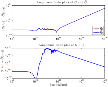
Fig. 2: Amplitude plots of ${\mathbf{G}}(\imath\omega)$ and ${\widetilde{{\mathbf{G}}}}(\imath\omega)$ (upper); the absolute error $|{\mathbf{G}}(\imath\omega)-{\widetilde{{\mathbf{G}}}}(\imath\omega)|$ (lower).

In some applications, the deflating subspaces of $\lambda{\mathbf{E}}-{\mathbf{A}}$ corresponding to the eigenvalues at infinity may have large dimension $n_{\infty}$. However, the order of the system can still be reduced if it contains states that are uncontrollable and unobservable at infinity. Such states can be removed from the system without changing its transfer function and, hence, preserving the interpolation conditions as in Theorem 2. In this case the projection matrices ${\mathbf{W}}_{\infty}$ and ${\mathbf{V}}_{\infty}$ can be determined as proposed in [26] by solving the projected discrete-time Lyapunov equations

$${\mathbf{A}}{\mathbf{X}}{\mathbf{A}}^{T}-{\mathbf{E}}{\mathbf{X}}{\mathbf{E}}^{T}\!=-({\mathbf{I}}-{\mathbf{P}}_{l}){\mathbf{B}}{\mathbf{B}}^{T}\!({\mathbf{I}}-{\mathbf{P}}_{l})^{T},\;\,{\mathbf{X}}=({\mathbf{I}}-{\mathbf{P}}_{r}){\mathbf{X}}({\mathbf{I}}-{\mathbf{P}}_{r})^{T},\enskip$$ (21)

$${\mathbf{A}}^{T}{\mathbf{Y}}{\mathbf{A}}-{\mathbf{E}}^{T}{\mathbf{Y}}{\mathbf{E}}=-({\mathbf{I}}-{\mathbf{P}}_{r})^{T}{\mathbf{C}}^{T}\!{\mathbf{C}}({\mathbf{I}}-{\mathbf{P}}_{r}),\;{\mathbf{Y}}=({\mathbf{I}}-{\mathbf{P}}_{l})^{T}{\mathbf{Y}}({\mathbf{I}}-{\mathbf{P}}_{l}).\enskip$$ (22)

Let ${\mathbf{X}}_{C}$ and ${\mathbf{Y}}_{C}$ be the Cholesky factors of ${\mathbf{X}}={\mathbf{X}}_{C}{\mathbf{X}}_{C}^{T}$ and ${\mathbf{Y}}={\mathbf{Y}}_{C}{\mathbf{Y}}_{C}^{T}$, respectively, and let ${\mathbf{Y}}_{C}^{T}{\mathbf{A}}{\mathbf{X}}_{C}=[{\mathbf{U}}_{1},\,{\mathbf{U}}_{0}]\mbox{\rm diag}(\mathbf{\Sigma},\mathbf{0})[{\mathbf{V}}_{1},\,{\mathbf{V}}_{0}]^{T}$ be singular value decomposition, where $[{\mathbf{U}}_{1},\,{\mathbf{U}}_{0}]$ and $[{\mathbf{V}}_{1},\,{\mathbf{V}}_{0}]$ are orthogonal and $\mathbf{\Sigma}$ is nonsingular. Then the projection matrices ${\mathbf{W}}_{\infty}$ and ${\mathbf{V}}_{\infty}$ can be taken as ${\mathbf{W}}_{\infty}={\mathbf{Y}}_{C}{\mathbf{U}}_{1}$ and ${\mathbf{V}}_{\infty}={\mathbf{X}}_{C}{\mathbf{V}}_{1}$. Note that the Cholesky factors ${\mathbf{X}}_{C}$ and ${\mathbf{Y}}_{C}$ can be computed directly using the generalized Smith method [27]. In this method, it is required to solve $\nu-1$ linear systems only, where $\nu$ is the index of the pencil $\lambda{\mathbf{E}}-{\mathbf{A}}$ or, equivalently, the nilpotence index of ${\mathbf{N}}$ in (14). The computation of the projectors ${\mathbf{P}}_{l}$ and ${\mathbf{P}}_{r}$ is, in general, a difficult problem. However, for some structured problems arising in circuit simulation, multibody systems and computational fluid dynamics, these projectors can be constructed in explicit form that significantly reduces the computational complexity of the method; see [27] for details.

4 Interpolatory optimal ${{\mathcal{H}}_{2}}$ model reduction for descriptor systems

The choice of interpolation points and tangential directions is the central issue in interpolatory model reduction. This choice determines whether the reduced-order model is high fidelity or not. Until recently, selection of interpolation points was largely ad hoc and required several model reduction attempts to arrive at a reasonable approximation. However, Gugercin et al. [15] introduced an interpolatory model reduction method for generating a reduced model ${\widetilde{{\mathbf{G}}}}$ of order $r$ which is an optimal ${\mathcal{H}}_{2}$ approximation to the original system ${\mathbf{G}}$ in the sense that it minimizes ${{\mathcal{H}}_{2}}$-norm error, i.e.,

$$\|{\mathbf{G}}-{\widetilde{{\mathbf{G}}}}\|_{{{\mathcal{H}}_{2}}}=\min_{{\small\dim({\widetilde{{\mathbf{G}}}}_{r})=r}}\|{\mathbf{G}}-{\widetilde{{\mathbf{G}}}}_{r}\|_{{{\mathcal{H}}_{2}}},$$ (23)

where

$$\left\|{\mathbf{G}}\right\|_{{{\mathcal{H}}_{2}}}:=\left(\frac{1}{2\pi}\int_{-\infty}^{+\infty}\|{\mathbf{G}}(\imath\omega)\|_{\rm F}^{2}\,d\omega\right)^{1/2}$$ (24)

and $\|\cdot\|_{\rm F}$ denotes the Frobenius matrix norm. Since this is a non-convex optimization problem, the computation of a global minimizer is a very difficult task. Hence, instead, one tries to find high-fidelity reduced models that satisfy first-order necessary optimality conditions. There exist, in general, two approaches for solving this problem. These are Lyapunov-based optimal ${{\mathcal{H}}_{2}}$ methods presented in [16, 18, 25, 29, 30, 33] and interpolation-based optimal ${{\mathcal{H}}_{2}}$ methods considered in [3, 4, 6, 12, 14, 15, 19, 23, 28]. While the Lyapunov-based approaches require solving a series of Lyapunov equations, which becomes costly and sometimes intractable in large-scale settings, the interpolatory approaches only require solving a series of sparse linear systems and have proved to be numerically very effective. Moreover, as shown in [15], both frameworks are theoretically equivalent that further motivates the usage of interpolatory model reduction techniques for the optimal ${{\mathcal{H}}_{2}}$ approximation.

For SISO systems, interpolation-based ${{\mathcal{H}}_{2}}$ optimality conditions were originally developed by Meier and Luenberger [23]. Then, based on these conditions, an effective algorithm for interpolatory optimal ${{\mathcal{H}}_{2}}$ approximation, called the Iterative Rational Krylov Algorithm (IRKA), was introduced in [12, 14]. This algorithm has also been recently extended to MIMO systems using the tangential interpolation framework, see [6, 15, 28] for more details.

The model reduction methods mentioned above, however, only deals with the system ${\mathbf{G}}(s)={\mathbf{C}}(s{\mathbf{E}}-{\mathbf{A}})^{-1}{\mathbf{B}}+{\mathbf{D}}$ with a nonsingular matrix ${\mathbf{E}}$. In this section, we will extend IRKA to descriptor systems. First, we establish the interpolatory ${{\mathcal{H}}_{2}}$ optimality conditions in the new setting.

Theorem 3.

Let ${\mathbf{G}}(s)={{\mathbf{G}}}_{\rm sp}(s)+{{\mathbf{P}}}(s)$ be decomposed into the strictly proper and polynomial parts, and let ${\widetilde{{\mathbf{G}}}}(s)={\widetilde{{\mathbf{G}}}_{\rm sp}}(s)+{\widetilde{{\mathbf{P}}}}(s)$ have an $r^{\rm th}$-order strictly proper part ${\widetilde{{\mathbf{G}}}_{\rm sp}}(s)={\widetilde{{\mathbf{C}}}}_{\rm sp}(s{\widetilde{{\mathbf{E}}}}_{\rm sp}-{\widetilde{{\mathbf{A}}}}_{\rm sp})^{-1}{\widetilde{{\mathbf{B}}}}_{\rm sp}$.

1. If ${\widetilde{{\mathbf{G}}}}(s)$ minimizes the ${{\mathcal{H}}_{2}}$-error $\|{\mathbf{G}}-{\widetilde{{\mathbf{G}}}}\|_{\mathcal{H}_{2}}$ over all reduced-order models with an $r^{\rm th}$-order strictly proper part, then ${\widetilde{{\mathbf{P}}}}(s)={{\mathbf{P}}}(s)$ and ${\widetilde{{\mathbf{G}}}_{\rm sp}}(s)$ minimizes the ${{\mathcal{H}}_{2}}$-error $\|{{\mathbf{G}}}_{\rm sp}-{\widetilde{{\mathbf{G}}}_{\rm sp}}\|_{\mathcal{H}_{2}}$.

2. Suppose that the pencil $s{{\widetilde{{\mathbf{E}}}}_{\rm sp}}-{{\widetilde{{\mathbf{A}}}}_{\rm sp}}$ has distinct eigenvalues $\{\widetilde{\lambda}_{i}\}_{i=1}^{r}$. Let ${\mathbf{y}}_{i}$ and ${\mathbf{z}}_{i}$ denote the left and right eigenvectors associated with $\tilde{\lambda}_{i}$ so that ${{\widetilde{{\mathbf{A}}}}_{\rm sp}}{\mathbf{z}}_{i}=\!\widetilde{\lambda}_{i}{{\widetilde{{\mathbf{E}}}}_{\rm sp}}{\mathbf{z}}_{i}$, ${\mathbf{y}}_{i}^{*}{{\widetilde{{\mathbf{A}}}}_{\rm sp}}=\!\widetilde{\lambda}_{i}{\mathbf{y}}_{i}^{*}{{\widetilde{{\mathbf{E}}}}_{\rm sp}}$, and ${\mathbf{y}}_{i}^{*}{{\widetilde{{\mathbf{E}}}}_{\rm sp}}{\mathbf{z}}_{j}=\delta_{ij}$. Then for $\mathbf{\mathsf{c}}_{i}={{\widetilde{{\mathbf{C}}}}_{\rm sp}}{\mathbf{z}}_{i}$ and $\mathbf{\mathsf{b}}_{i}^{T}={\mathbf{y}}_{i}^{*}{{\widetilde{{\mathbf{B}}}}_{\rm sp}}$, we have

   $$\begin{array}[]{c}{\mathbf{G}}(-\widetilde{\lambda}_{i})\mathbf{\mathsf{b}}_{i}={\widetilde{{\mathbf{G}}}}(-\widetilde{\lambda}_{i})\mathbf{\mathsf{b}}_{i},\qquad\mathbf{\mathsf{c}}_{i}^{T}{\mathbf{G}}(-\widetilde{\lambda}_{i})=\mathbf{\mathsf{c}}_{i}^{T}{\widetilde{{\mathbf{G}}}}(-\widetilde{\lambda}_{i}),\\[2.84526pt] \mbox{and}\quad\mathbf{\mathsf{c}}_{i}^{T}{\mathbf{G}}^{\prime}(-\widetilde{\lambda}_{i})\mathbf{\mathsf{b}}_{i}=\mathbf{\mathsf{c}}_{i}^{T}{\widetilde{{\mathbf{G}}}}^{\prime}(-\widetilde{\lambda}_{i})\mathbf{\mathsf{b}}_{i}\quad\mbox{for}\enskip i=1,\cdots,r.\end{array}$$ (25)

Proof.

1. The polynomial part of ${\mathbf{G}}(s)$ and ${\widetilde{{\mathbf{G}}}}(s)$ coincide, since, otherwise, the ${{\mathcal{H}}_{2}}$-norm of the error ${\mathbf{G}}(s)-{\widetilde{{\mathbf{G}}}}(s)$ would be unbounded. Then it readily follows that ${\widetilde{{\mathbf{G}}}_{\rm sp}}(s)$ minimizes $\|{{\mathbf{G}}}_{\rm sp}(s)-{\widetilde{{\mathbf{G}}}_{\rm sp}}(s)\|_{\mathcal{H}_{2}}$ since ${\mathbf{G}}(s)-{\widetilde{{\mathbf{G}}}}(s)={{\mathbf{G}}}_{\rm sp}(s)-{\widetilde{{\mathbf{G}}}_{\rm sp}}(s)$.

2. Since ${\widetilde{{\mathbf{P}}}}(s)={{\mathbf{P}}}(s)$, the ${{\mathcal{H}}_{2}}$ optimal model reduction problem for ${\mathbf{G}}(s)$ now reduces to the ${{\mathcal{H}}_{2}}$ optimal problem for the strictly proper transfer function ${{\mathbf{G}}}_{\rm sp}(s)$. Hence, the optimal ${{\mathcal{H}}_{2}}$ conditions of [15] require that ${\widetilde{{\mathbf{G}}}_{\rm sp}}(s)$ needs to be a bi-tangential Hermite interpolant to ${{\mathbf{G}}}_{\rm sp}(s)$ with $\{-\widetilde{\lambda}_{i}\}_{i=1}^{r}$ being the interpolation points, and $\{\mathbf{\mathsf{c}}_{i}\}_{i=1}^{r}$ and $\{\mathbf{\mathsf{b}}_{i}\}_{i=1}^{r}$ being the corresponding left and right tangential directions, respectively. Thus, the interpolation conditions (25) hold since ${\widetilde{{\mathbf{P}}}}(s)={{\mathbf{P}}}(s)$. ∎

Unfortunately, the ${{\mathcal{H}}_{2}}$ optimal interpolation points and associated tangent directions are not known a priori, since they depend on the reduced-order model to be computed. To overcome this difficulty, an iterative algorithm IRKA was developed [12, 14] which is based on successive substitution. In IRKA, the interpolation points are corrected iteratively by the choosing mirror images of poles of the current reduced-order model as the next interpolation points. The tangential directions are corrected in a similar way; see [1, 15] for details.

The situation in the case of descriptor systems is similar, where the optimal interpolation points and the corresponding tangential directions depend on the strictly proper part of the reduced-order model to be computed. Moreover, we need to make sure that the final reduced-model has the same polynomial part as the original one. Hence, we will modify IRKA to meet these challenges. In particular, we will correct not the poles and the tangential directions of the intermediate reduced-order model at the successive iteration step but that of the strictly proper part of the intermediate reduced-order model. As in the case of Theorem 2, the spectral projectors ${\mathbf{P}}_{l}$ and ${\mathbf{P}}_{r}$ will be used to construct the required interpolatory subspaces. A sketch of the resulting model reduction method is given in Algorithm 4.1.

Algorithm 4.1.

Interpolatory ${{\mathcal{H}}_{2}}$ optimal model reduction method
                        for descriptor systems 1) Make an initial selection of the interpolation points $\{\sigma_{i}\}_{i=1}^{r}$ and the
tangential directions $\{\mathbf{\mathsf{b}}_{i}\}_{i=1}^{r}$ and $\{\mathbf{\mathsf{c}}_{i}\}_{i=1}^{r}$. 2) $\;{\mathbf{V}}_{\!f}=\left[\,(\sigma_{1}{\mathbf{E}}-{\mathbf{A}})^{-1}{\mathbf{P}}_{l}{\mathbf{B}}\mathbf{\mathsf{b}}_{1},\;\ldots,\;(\sigma_{r}{\mathbf{E}}-{\mathbf{A}})^{-1}{\mathbf{P}}_{l}{\mathbf{B}}\mathbf{\mathsf{b}}_{r}\,\right]$,
${\mathbf{W}}_{\!f}=\left[\,({\sigma_{1}}{\mathbf{E}}-{\mathbf{A}})^{-T}{\mathbf{P}}_{r}^{T}{\mathbf{C}}^{T}\mathbf{\mathsf{c}}_{1},\;\ldots,\;({\sigma_{r}}{\mathbf{E}}-{\mathbf{A}})^{-T}{\mathbf{P}}_{r}^{T}{\mathbf{C}}^{T}\mathbf{\mathsf{c}}_{r}\,\right]$. 3) while (not converged) a) ${{\widetilde{{\mathbf{A}}}}_{\rm sp}}={\mathbf{W}}_{\!f}^{T}{\mathbf{A}}{\mathbf{V}}_{\!f}$, ${{\widetilde{{\mathbf{E}}}}_{\rm sp}}={\mathbf{W}}_{\!f}^{T}{\mathbf{E}}{\mathbf{V}}_{\!f}$, ${{\widetilde{{\mathbf{B}}}}_{\rm sp}}={\mathbf{W}}_{\!f}^{T}{\mathbf{B}}$, and ${{\widetilde{{\mathbf{C}}}}_{\rm sp}}={\mathbf{C}}{\mathbf{V}}_{\!f}$. b) Compute ${{\widetilde{{\mathbf{A}}}}_{\rm sp}}{\mathbf{z}}_{i}=\widetilde{\lambda}_{i}{{\widetilde{{\mathbf{E}}}}_{\rm sp}}{\mathbf{z}}_{i}$ and ${\mathbf{y}}_{i}^{*}{{\widetilde{{\mathbf{A}}}}_{\rm sp}}=\widetilde{\lambda}_{i}{\mathbf{y}}_{i}^{*}{{\widetilde{{\mathbf{E}}}}_{\rm sp}}$ with ${\mathbf{y}}_{i}^{*}{{\widetilde{{\mathbf{E}}}}_{\rm sp}}{\mathbf{z}}_{j}=\delta_{ij}$,
where ${\mathbf{y}}_{i}$ and ${\mathbf{z}}_{i}$ are left and right eigenvectors associated with $\widetilde{\lambda}_{i}$. c) $\sigma_{i}\leftarrow-\widetilde{\lambda}_{i}$, $\mathbf{\mathsf{b}}_{i}^{T}\leftarrow{\mathbf{y}}_{i}^{*}{{\widetilde{{\mathbf{B}}}}_{\rm sp}}$ and $\mathbf{\mathsf{c}}_{i}\leftarrow{{\widetilde{{\mathbf{C}}}}_{\rm sp}}{\mathbf{z}}_{i}$ for $i=1,\ldots,r$. d) $\;{\mathbf{V}}_{\!f}=\left[\,(\sigma_{1}{\mathbf{E}}-{\mathbf{A}})^{-1}{\mathbf{P}}_{l}{\mathbf{B}}\mathbf{\mathsf{b}}_{1},\;\ldots,\;(\sigma_{r}{\mathbf{E}}-{\mathbf{A}})^{-1}{\mathbf{P}}_{l}{\mathbf{B}}\mathbf{\mathsf{b}}_{r}\,\right]$,
${\mathbf{W}}_{\!f}=\left[\,({\sigma_{1}}{\mathbf{E}}-{\mathbf{A}})^{-T}{\mathbf{P}}_{r}^{T}{\mathbf{C}}^{T}\mathbf{\mathsf{c}}_{1},\;\ldots,\;({\sigma_{r}}{\mathbf{E}}-{\mathbf{A}})^{-T}{\mathbf{P}}_{r}^{T}{\mathbf{C}}^{T}\mathbf{\mathsf{c}}_{r}\,\right]$. end while 4) Compute ${\mathbf{W}}_{\infty}$ and ${\mathbf{V}}_{\infty}$ such that $\mbox{\rm Im}({\mathbf{W}}_{\infty})=\mbox{\rm Im}({\mathbf{I}}-{\mathbf{P}}_{l}^{T})$ and
$\mbox{\rm Im}({\mathbf{V}}_{\infty})=\mbox{\rm Im}({\mathbf{I}}-{\mathbf{P}}_{r})$. 5) Set ${\mathbf{V}}=[\,{\mathbf{V}}_{\!f},\;{\mathbf{V}}_{\infty}\,]$ and ${\mathbf{W}}=[\,{\mathbf{W}}_{\!f},\;{\mathbf{W}}_{\infty}\,]$. 6) ${\widetilde{{\mathbf{E}}}}={\mathbf{W}}^{T}{\mathbf{E}}{\mathbf{V}}$, ${\widetilde{{\mathbf{A}}}}={\mathbf{W}}^{T}{\mathbf{A}}{\mathbf{V}}$, ${\widetilde{{\mathbf{B}}}}={\mathbf{W}}^{T}{\mathbf{B}}$, ${\widetilde{{\mathbf{C}}}}={\mathbf{C}}{\mathbf{V}}$, ${\widetilde{{\mathbf{D}}}}={\mathbf{D}}$.

Note that until Step 4 of Algorithm 4.1, the polynomial part is not included since the interpolation parameters result from the strictly proper part ${\widetilde{{\mathbf{G}}}_{\rm sp}}(s)$. In a sense, Step 3 runs the optimal ${{\mathcal{H}}_{2}}$ iteration on ${{\mathbf{G}}}_{\rm sp}(s)$. Hence, at the end of Step 3, we construct an optimal ${{\mathcal{H}}_{2}}$ interpolant to ${{\mathbf{G}}}_{\rm sp}(s)$. However, in Step 5, we append the interpolatory subspaces with ${\mathbf{V}}_{\infty}$ and ${\mathbf{W}}_{\infty}$ (which can be computed as described at the end of Section 3) so that the final reduced-order model in Step 6 has the same polynomial part as ${\mathbf{G}}(s)$, and, consequently, the final reduced-order model ${\widetilde{{\mathbf{G}}}}(s)$ satisfies the optimality conditions of Theorem 3. One can see this from Step 3c: upon convergence, the interpolation points are the mirror images of the poles of ${\widetilde{{\mathbf{G}}}_{\rm sp}}(s)$ and the tangential directions are the residue directions from ${\widetilde{{\mathbf{G}}}_{\rm sp}}(s)$ as the optimality conditions require. Since Algorithm 4.1 uses the projected quantities ${\mathbf{P}}_{l}{\mathbf{B}}$ and ${\mathbf{C}}{\mathbf{P}}_{r}$, theoretically iterating on a strictly proper dynamical system, the convergence behavior of this algorithm will follow the same pattern of IRKA which has been observed to converge rapidly in numerous numerical applications.

Summarizing, we have shown so far how to reduce descriptor systems such that the transfer function of the reduced descriptor systems is a tangential interpolant to the original one and matches the polynomial part preventing unbounded ${{\mathcal{H}}_{\infty}}$ and ${{\mathcal{H}}_{2}}$ error norms. However, this model reduction approach involves the explicit computation of the spectral projectors or the corresponding deflating subspaces, which could be numerically infeasible for general large-scale problems. In the next two sections, we will show that for certain important classes of descriptor systems, the same can be achieved without explicitly forming the spectral projectors.

5 Semi-explicit descriptor systems of index 1

We consider the following semi-explicit descriptor system

$$\begin{array}[]{rcl}{\mathbf{E}}_{11}\dot{{\mathbf{x}}}_{1}(t)+{\mathbf{E}}_{12}\dot{{\mathbf{x}}}_{2}(t)&=&{\mathbf{A}}_{11}{\mathbf{x}}_{1}(t)+{\mathbf{A}}_{12}{\mathbf{x}}_{2}(t)+{\mathbf{B}}_{1}{\mathbf{u}}(t),\\ \mathbf{0}&=&{\mathbf{A}}_{21}{\mathbf{x}}_{1}(t)+{\mathbf{A}}_{22}{\mathbf{x}}_{2}(t)+{\mathbf{B}}_{2}{\mathbf{u}}(t),\\ {\mathbf{y}}(t)&=&{\mathbf{C}}_{1}{\mathbf{x}}_{1}(t)+{\mathbf{C}}_{2}{\mathbf{x}}_{2}(t)+{\mathbf{D}}{\mathbf{u}}(t),\\ \end{array}$$ (26)

where the state is ${\mathbf{x}}(t)=[\,{\mathbf{x}}_{1}^{T}(t),\;{\mathbf{x}}_{2}^{T}(t)\,]^{T}\in\mbox{\Bb R}^{n}$ with ${\mathbf{x}}_{1}(t)\in\mbox{\Bb R}^{n_{1}}$, ${\mathbf{x}}_{2}(t)\in\mbox{\Bb R}^{n_{2}}$ and $n_{1}+n_{2}=n$, the input is ${\mathbf{u}}(t)\in\mbox{\Bb R}^{m}$, the output is ${\mathbf{y}}(t)\in\mbox{\Bb R}^{p}$, and ${\mathbf{E}}_{11},{\mathbf{A}}_{11}\in\mbox{\Bb R}^{n_{1}\times n_{1}}$, ${\mathbf{E}}_{12},{\mathbf{A}}_{12}\in\mbox{\Bb R}^{n_{1}\times n_{2}}$, ${\mathbf{A}}_{21}\in\mbox{\Bb R}^{n_{2}\times n_{1}}$, ${\mathbf{A}}_{22}\in\mbox{\Bb R}^{n_{2}\times n_{2}}$, ${\mathbf{B}}_{1}\in\mbox{\Bb R}^{n_{1}\times m}$, ${\mathbf{B}}_{2}\in\mbox{\Bb R}^{n_{2}\times m}$, ${\mathbf{C}}_{1}\in\mbox{\Bb R}^{p\times n_{1}}$, ${\mathbf{C}}_{2}\in\mbox{\Bb R}^{p\times n_{2}}$, ${\mathbf{D}}\in\mbox{\Bb R}^{p\times m}$. We assume that ${\mathbf{A}}_{22}$ and ${\mathbf{E}}_{11}-{\mathbf{E}}_{12}{\mathbf{A}}^{-1}_{22}{\mathbf{A}}_{21}$ are both nonsingular. In this case system (26) is of index 1. We now compute the polynomial part of this system.

Proposition 4.

Let ${\mathbf{G}}(s)$ be a transfer function of the descriptor system (26), where ${\mathbf{A}}_{22}$ and ${\mathbf{E}}_{11}-{\mathbf{E}}_{12}{\mathbf{A}}^{-1}_{22}{\mathbf{A}}_{21}$ are both nonsingular. Then the polynomial part of ${\mathbf{G}}(s)$ is a constant matrix given by

$${\mathbf{P}}(s)={\mathbf{C}}_{1}{\mathbf{M}}_{1}{\mathbf{B}}_{2}+{\mathbf{C}}_{2}{\mathbf{M}}_{2}{\mathbf{B}}_{2}+{\mathbf{D}},$$

where

$${\mathbf{M}}_{1} = ({\mathbf{E}}_{11}-{\mathbf{E}}_{12}{\mathbf{A}}^{-1}_{22}{\mathbf{A}}_{21})^{-1}{\mathbf{E}}_{12}{\mathbf{A}}^{-1}_{22},$$ (27)

$${\mathbf{M}}_{2} = -{\mathbf{A}}^{-1}_{22}{\mathbf{A}}_{21}({\mathbf{E}}_{11}-{\mathbf{E}}_{12}{\mathbf{A}}^{-1}_{22}{\mathbf{A}}_{21})^{-1}{\mathbf{E}}_{12}{\mathbf{A}}^{-1}_{22}-{\mathbf{A}}_{22}^{-1}.$$ (28)

Proof.

Consider

$$(s{\mathbf{E}}-{\mathbf{A}})^{-1}{\mathbf{B}}=\left[\begin{array}[]{cc}s{\mathbf{E}}_{11}-{\mathbf{A}}_{11}&s{\mathbf{E}}_{12}-{\mathbf{A}}_{12}\\ -{\mathbf{A}}_{21}&-{\mathbf{A}}_{22}\end{array}\right]^{-1}\left[\begin{array}[]{c}{\mathbf{B}}_{1}\\ {\mathbf{B}}_{2}\end{array}\right]=\left[\begin{array}[]{c}{\mathbf{F}}_{1}(s)\\ {\mathbf{F}}_{2}(s)\end{array}\right].$$

This leads to

$$(s{\mathbf{E}}_{11}-{\mathbf{A}}_{11}){\mathbf{F}}_{1}(s)+(s{\mathbf{E}}_{12}-{\mathbf{A}}_{12}){\mathbf{F}}_{2}(s) = {\mathbf{B}}_{1},$$ (29)

$$-{\mathbf{A}}_{21}{\mathbf{F}}_{1}(s)-{\mathbf{A}}_{22}{\mathbf{F}}_{2}(s) = {\mathbf{B}}_{2}.$$ (30)

Solving (30) for ${\mathbf{F}}_{2}(s)$ gives ${\mathbf{F}}_{2}(s)=-{\mathbf{A}}_{22}^{-1}({\mathbf{B}}_{2}+{\mathbf{A}}_{21}{\mathbf{F}}_{1}(s))$, and, thus,

$${\mathbf{F}}_{1}(s)=\left((s{\mathbf{E}}_{11}-{\mathbf{A}}_{11})-(s{\mathbf{E}}_{12}-{\mathbf{A}}_{12}){\mathbf{A}}_{22}^{-1}{\mathbf{A}}_{21}\right)^{-1}\left({\mathbf{B}}_{1}+(s{\mathbf{E}}_{12}-{\mathbf{A}}_{12}){\mathbf{A}}_{22}^{-1}{\mathbf{B}}_{2}\right)$$

implying that

$$\lim_{s\rightarrow\infty}{\mathbf{F}}_{1}(s)=\left({\mathbf{E}}_{11}-{\mathbf{E}}_{12}{\mathbf{A}}_{22}^{-1}{\mathbf{A}}_{21}\right)^{-1}{\mathbf{E}}_{12}{\mathbf{A}}_{22}^{-1}{\mathbf{B}}_{2}.$$

Taking into account (30), we have

$$\lim_{s\rightarrow\infty}{\mathbf{F}}_{2}(s)=\left[-{\mathbf{A}}_{22}^{-1}{\mathbf{A}}_{21}\left({\mathbf{E}}_{11}-{\mathbf{E}}_{12}{\mathbf{A}}_{22}^{-1}{\mathbf{A}}_{21}\right)^{-1}{\mathbf{E}}_{12}{\mathbf{A}}_{22}^{-1}-{\mathbf{A}}_{22}^{-1}\right]{\mathbf{B}}_{2}.$$

Finally, note that ${\mathbf{P}}(s)=\lim\limits_{s\rightarrow\infty}{\mathbf{G}}(s)=\lim\limits_{s\rightarrow\infty}({\mathbf{C}}_{1}{\mathbf{F}}_{1}(s)+{\mathbf{C}}_{2}{\mathbf{F}}_{2}(s)+{\mathbf{D}})$, which leads to the desired conclusion. ∎

We are now ready to state the interpolation result for the descriptor system (26). This result was briefly hinted at in the recent survey [1]. Here, we present it with a formal proof together with the formula developed for ${\mathbf{P}}(s)$ in Proposition 4. As our main focus will be ${{\mathcal{H}}_{2}}$-based model reduction, we will list the interpolation conditions only for the bi-tangential Hermite interpolation. Extension to the higher-order derivative interpolation is straightforward as shown in the earlier sections.

Lemma 5.

Let ${\mathbf{G}}(s)$ be a transfer function of the semi-explicit descriptor system (26). For given $r$ distinct interpolation points $\{\sigma_{i}\}_{i=1}^{r}$, left tangential directions $\{\mathbf{\mathsf{c}}_{i}\}_{i=1}^{r}$ and right tangential directions $\{\mathbf{\mathsf{b}}_{i}\}_{i=1}^{r}$, let ${\mathbf{V}}\in\mbox{\Bb C}^{n\times r}$ and ${\mathbf{W}}\in\mbox{\Bb C}^{n\times r}$ be given by

$${\mathbf{V}} = [\,(\sigma_{1}{\mathbf{E}}-{\mathbf{A}})^{-1}{\mathbf{B}}\mathbf{\mathsf{b}}_{1},\;\ldots,\;(\sigma_{r}{\mathbf{E}}-{\mathbf{A}})^{-1}{\mathbf{B}}\mathbf{\mathsf{b}}_{r}\,],$$ (31)

$${\mathbf{W}} = [\,(\sigma_{1}{\mathbf{E}}-{\mathbf{A}})^{-T}{\mathbf{C}}^{T}\mathbf{\mathsf{c}}_{1},\;\ldots,\;(\sigma_{r}{\mathbf{E}}-{\mathbf{A}})^{-T}{\mathbf{C}}^{T}\mathbf{\mathsf{c}}_{r}\,].$$ (32)

Furthermore, let $\mathcal{B}$ and $\mathcal{C}$ be the matrices composed of the tangential directions as

$$\mathcal{B}=[\,\mathbf{\mathsf{b}}_{1},\,\ldots,\,\mathbf{\mathsf{b}}_{r}\,]\qquad\text{and}\qquad\mathcal{C}=[\,\mathbf{\mathsf{c}}_{1},\,\ldots,\,\mathbf{\mathsf{c}}_{r}\,].$$ (33)

Define the reduced-order system matrices as

$$\begin{array}[]{ll}{\widetilde{{\mathbf{E}}}}={\mathbf{W}}^{T}{\mathbf{E}}{\mathbf{V}},&\quad{\widetilde{{\mathbf{A}}}}={\mathbf{W}}^{T}{\mathbf{A}}{\mathbf{V}}+\mathcal{C}^{T}{\widetilde{{\mathbf{D}}}}\mathcal{B},\quad{\widetilde{{\mathbf{B}}}}={\mathbf{W}}^{T}{\mathbf{B}}-\mathcal{C}^{T}{\widetilde{{\mathbf{D}}}},\\[7.22743pt] {\widetilde{{\mathbf{C}}}}={\mathbf{C}}{\mathbf{V}}-{\widetilde{{\mathbf{D}}}}\mathcal{B},&\quad{\widetilde{{\mathbf{D}}}}={\mathbf{C}}_{1}{\mathbf{M}}_{1}{\mathbf{B}}_{2}+{\mathbf{C}}_{2}{\mathbf{M}}_{2}{\mathbf{B}}_{2}+{\mathbf{D}}.\end{array}$$ (34)

Then the polynomial parts of ${\widetilde{{\mathbf{G}}}}(s)={\widetilde{{\mathbf{C}}}}(s{\widetilde{{\mathbf{E}}}}-{\widetilde{{\mathbf{A}}}})^{-1}{\widetilde{{\mathbf{B}}}}+{\widetilde{{\mathbf{D}}}}$ and ${\mathbf{G}}(s)$ match assuming ${\widetilde{{\mathbf{E}}}}$ is nonsingular, and ${\widetilde{{\mathbf{G}}}}(s)$ satisfies the bi-tangential Hermite interpolation conditions

$${\mathbf{G}}(\sigma_{i})\mathbf{\mathsf{b}}_{i}={\widetilde{{\mathbf{G}}}}(\sigma_{i})\mathbf{\mathsf{b}}_{i},\qquad\mathbf{\mathsf{c}}_{i}^{T}{\mathbf{G}}(\sigma_{i})=\mathbf{\mathsf{c}}_{i}^{T}{\widetilde{{\mathbf{G}}}}(\sigma_{i}),\qquad\mathbf{\mathsf{c}}_{i}^{T}{\mathbf{G}}^{\prime}(\sigma_{i})\mathbf{\mathsf{b}}_{i}=\mathbf{\mathsf{c}}_{i}^{T}{\widetilde{{\mathbf{G}}}}^{\prime}(\sigma_{i})\mathbf{\mathsf{b}}_{i}$$

for $i=1,\ldots,r$, provided $\sigma_{i}{\mathbf{E}}-{\mathbf{A}}$ and $\sigma_{i}{\widetilde{{\mathbf{E}}}}-{\widetilde{{\mathbf{A}}}}$ are both nonsingular.

Proof.

Since ${\widetilde{{\mathbf{E}}}}$ is nonsingular, $\lim\limits_{s\rightarrow\infty}{\widetilde{{\mathbf{G}}}}(s)={\widetilde{{\mathbf{D}}}}$. But by Lemma 4, we have $\widetilde{{\mathbf{D}}}=\lim\limits_{s\rightarrow\infty}{\mathbf{G}}(s)$ ensuring that the polynomial parts of ${\mathbf{G}}(s)$ and ${\widetilde{{\mathbf{G}}}}(s)$ coincide. The interpolation property is a result of [2, 22], where it is shown that the appropriate shifting of the reduced-order quantities with a non-zero feedthrough term as done in (34) attains the original bi-tangential interpolation conditions hidden in ${\mathbf{V}}$ and ${\mathbf{W}}$ of (31) and (32), respectively. ∎

This result leads to Algorithm 5.1, which achieves bi-tangential Hermite interpolation of the semi-explicit descriptor system (26) without explicitly forming the spectral projectors.

Algorithm 5.1.

Interpolatory model reduction for semi-explicit
                         descriptor systems of index 1 1) Make an initial selection of the interpolation points $\{\sigma_{i}\}_{i=1}^{r}$ and the tangential directions $\{{\mathbf{\mathsf{b}}}_{i}\}_{i=1}^{r}$ and $\{{\mathbf{\mathsf{c}}}_{i}\}_{i=1}^{r}$. 2) $\;{\mathbf{V}}=[\,(\sigma_{1}{\mathbf{E}}-{\mathbf{A}})^{-1}{\mathbf{B}}{\mathbf{\mathsf{b}}}_{1},\,\ldots,\,(\sigma_{r}{\mathbf{E}}-{\mathbf{A}})^{-1}{\mathbf{B}}{\mathbf{\mathsf{b}}}_{r}\,]$,
${\mathbf{W}}=[\,(\sigma_{1}{\mathbf{E}}-{\mathbf{A}})^{-T}{\mathbf{C}}^{T}\mathbf{\mathsf{c}}_{1},\,\ldots,\,(\sigma_{r}{\mathbf{E}}-{\mathbf{A}})^{-T}{\mathbf{C}}^{T}\mathbf{\mathsf{c}}_{r}\,]$. 3) Define ${\widetilde{{\mathbf{D}}}}={\mathbf{C}}_{1}{\mathbf{M}}_{1}{\mathbf{B}}_{2}+{\mathbf{C}}_{2}{\mathbf{M}}_{2}{\mathbf{B}}_{2}+{\mathbf{D}}$, where ${\mathbf{M}}_{1}$ and ${\mathbf{M}}_{2}$ are defined in (27) and (28), respectively. 4) Define $\mathcal{B}=\left[\,\mathbf{\mathsf{b}}_{1},\,\ldots,\,\mathbf{\mathsf{b}}_{r}\,\right]$ and $\mathcal{C}=\left[\,\mathbf{\mathsf{c}}_{1},\,\ldots,\,\mathbf{\mathsf{c}}_{r}\,\right]$. 5) ${\widetilde{{\mathbf{E}}}}={\mathbf{W}}^{T}{\mathbf{E}}{\mathbf{V}}$,  ${\widetilde{{\mathbf{A}}}}={\mathbf{W}}^{T}{\mathbf{A}}{\mathbf{V}}+\mathcal{C}^{T}{\widetilde{{\mathbf{D}}}}\mathcal{B}$,  ${\widetilde{{\mathbf{B}}}}={\mathbf{W}}^{T}{\mathbf{B}}-\mathcal{C}^{T}{\widetilde{{\mathbf{D}}}}$,  ${\widetilde{{\mathbf{C}}}}={\mathbf{C}}{\mathbf{V}}-{\widetilde{{\mathbf{D}}}}\mathcal{B}$.

We want to emphasize that the assumption in Lemma 5 that ${\widetilde{{\mathbf{E}}}}$ be nonsingular is not restrictive. This will be the case generically. If ${\mathbf{W}}$ and ${\mathbf{V}}$ are full-rank $n\times r$ matrices, the rank of the $r\times r$ matrix ${\widetilde{{\mathbf{E}}}}={\mathbf{W}}^{T}{\mathbf{E}}{\mathbf{V}}$ will be generically $r$ as long as $rank({\mathbf{E}})>r$. The fact that ${\widetilde{{\mathbf{E}}}}$ will be full-rank is indeed the precise reason why we cannot simply apply Theorem 1 to descriptor systems.

5.1 Optimal ${{\mathcal{H}}_{2}}$ model reduction for semi-explicit descriptor systems

Lemma 5 provides the theoretical basis for an IRKA-based iteration for ${{\mathcal{H}}_{2}}$ model reduction of semi-explicit descriptor systems. One naive approach would be the following: Given system (26), simply apply IRKA of [15] to obtain an intermediate reduced-order model $\widehat{{\mathbf{G}}}(s)=\widehat{{\mathbf{C}}}(s\widehat{{\mathbf{E}}}-\widehat{{\mathbf{A}}})^{-1}\widehat{{\mathbf{B}}}+\widehat{{\mathbf{D}}}$. Of course, this will be generically an ODE and will not necessarily match the behavior of ${\mathbf{G}}(s)$ around $s=\infty$. Thus, apply Lemma 5 to obtain the final reduced-model ${\widetilde{{\mathbf{G}}}}(s)={\widetilde{{\mathbf{C}}}}(s{\widetilde{{\mathbf{E}}}}-{\widetilde{{\mathbf{A}}}})^{-1}{\widetilde{{\mathbf{B}}}}+\widetilde{{\mathbf{D}}}$ with

$${\widetilde{{\mathbf{E}}}}=\widehat{{\mathbf{E}}},\quad{\widetilde{{\mathbf{A}}}}=\widehat{{\mathbf{A}}}+\mathcal{C}^{T}{\widetilde{{\mathbf{D}}}}\mathcal{B},\quad{\widetilde{{\mathbf{B}}}}=\widehat{{\mathbf{B}}}-\mathcal{C}^{T}{\widetilde{{\mathbf{D}}}},\quad{\widetilde{{\mathbf{C}}}}=\widehat{{\mathbf{C}}}-{\widetilde{{\mathbf{D}}}}\mathcal{B},$$ (35)

where ${\widetilde{{\mathbf{D}}}}$ is defined as in Lemma 5. While this shifting of the intermediate matrices by the ${\mathbf{D}}$-term guarantees that the polynomial parts of ${\mathbf{G}}(s)$ and ${\widetilde{{\mathbf{G}}}}(s)$ match, the ${{\mathcal{H}}_{2}}$ optimality conditions will not be satisfied. The reason is as follows. Recall that the ${{\mathcal{H}}_{2}}$ optimality requires bi-tangential Hermite interpolation at the mirror images of the reduced-order poles. The intermediate model $\widehat{{\mathbf{G}}}(s)$ satisfies this but since it does not match the polynomial part, the resulting ${{\mathcal{H}}_{2}}$ error is unbounded. Then constructing ${\widetilde{{\mathbf{G}}}}(s)$ as in (35), we enforce the matching of the polynomial part but ${\widetilde{{\mathbf{G}}}}(s)$ still interpolates ${\mathbf{G}}(s)$ at the same interpolation points as $\widehat{{\mathbf{G}}}(s)$, i.e., at the mirror images of the poles of $\widehat{{\mathbf{G}}}(s)$. However, clearly due to (35), the poles of $\widehat{{\mathbf{G}}}(s)$ and ${\widetilde{{\mathbf{G}}}}(s)$ are different; thus ${\widetilde{{\mathbf{G}}}}(s)$ will no longer satisfy the optimal $\mathcal{H}_{2}$ necessary conditions. In order to achieve both the mirror-image interpolation conditions and the polynomial part matching, the ${\widetilde{{\mathbf{D}}}}$ term modification must be included throughout the iteration, not just at the end. This results in Algorithm 5.2.

Algorithm 5.2.

IRKA for semi-explicit descriptor systems of index 1 1) Make an initial shift selection $\{\sigma_{i}\}_{i=1}^{r}$ and initial tangential directions $\{{\mathbf{\mathsf{b}}}_{i}\}_{i=1}^{r}$ and $\{{\mathbf{\mathsf{c}}}_{i}\}_{i=1}^{r}$. 2) ${\mathbf{V}}_{r}=\left[\,(\sigma_{1}{\mathbf{E}}-{\mathbf{A}})^{-1}{\mathbf{B}}{\mathbf{\mathsf{b}}}_{1},\,\ldots,\,(\sigma_{r}{\mathbf{E}}-{\mathbf{A}})^{-1}{\mathbf{B}}{\mathbf{\mathsf{b}}}_{r}\,\right]$,
${\mathbf{W}}_{r}=\left[\,({\sigma_{1}}{\mathbf{E}}-{\mathbf{A}})^{-T}{\mathbf{C}}^{T}{\mathbf{\mathsf{c}}}_{1},\,\ldots,\,({\sigma_{r}}{\mathbf{E}}-{\mathbf{A}})^{-T}{\mathbf{C}}^{T}{\mathbf{\mathsf{c}}}_{r}\,\right]$. 3) Define ${\widetilde{{\mathbf{D}}}}={\mathbf{C}}_{1}{\mathbf{M}}_{1}{\mathbf{B}}_{2}+{\mathbf{C}}_{2}{\mathbf{M}}_{2}{\mathbf{B}}_{2}+{\mathbf{D}}$, where ${\mathbf{M}}_{1}$ and ${\mathbf{M}}_{2}$ are defined in (27) and (28), respectively. 4) Define $\mathcal{B}=\left[\,\mathbf{\mathsf{b}}_{1},\,\ldots,\,\mathbf{\mathsf{b}}_{r}\,\right]$ and $\mathcal{C}=\left[\,\mathbf{\mathsf{c}}_{1},\,\ldots,\,\mathbf{\mathsf{c}}_{r}\,\right]$. 5) while (not converged) a) ${\widetilde{{\mathbf{E}}}}={\mathbf{W}}^{T}{\mathbf{E}}{\mathbf{V}}$, ${\widetilde{{\mathbf{A}}}}={\mathbf{W}}^{T}{\mathbf{A}}{\mathbf{V}}+\mathcal{C}^{T}{\widetilde{{\mathbf{D}}}}\mathcal{B}$, ${\widetilde{{\mathbf{B}}}}={\mathbf{W}}^{T}{\mathbf{B}}-\mathcal{C}^{T}{\widetilde{{\mathbf{D}}}}$, ${\widetilde{{\mathbf{C}}}}={\mathbf{C}}{\mathbf{V}}-{\widetilde{{\mathbf{D}}}}\mathcal{B}$. b) Compute ${\mathbf{Y}}^{*}{\widetilde{{\mathbf{A}}}}{\mathbf{Z}}=\mbox{\rm diag}(\lambda_{1},\ldots,\lambda_{r})$ and ${\mathbf{Y}}^{*}{\widetilde{{\mathbf{E}}}}{\mathbf{Z}}={\mathbf{I}}_{r}$, where the columns of ${\mathbf{Z}}=[{\mathbf{z}}_{1},\ldots,{\mathbf{z}}_{r}]$ and ${\mathbf{Y}}=[{\mathbf{y}}_{1},\ldots,{\mathbf{y}}_{r}]$ are, respectively, the right and left eigenvectors of $\lambda{\widetilde{{\mathbf{E}}}}-{\widetilde{{\mathbf{A}}}}$. c) $\sigma_{i}\leftarrow-\lambda_{i}$, ${\mathbf{\mathsf{b}}}_{i}^{T}\leftarrow{\mathbf{y}}_{i}^{*}{\widetilde{{\mathbf{B}}}}$ and ${\mathbf{\mathsf{c}}}_{i}\leftarrow{\widetilde{{\mathbf{C}}}}{\mathbf{z}}_{i}$ for $i=1,\ldots,r$. d) ${\mathbf{V}}=\left[\,(\sigma_{1}{\mathbf{E}}-{\mathbf{A}})^{-1}{\mathbf{B}}{\mathbf{\mathsf{b}}}_{1},\,\ldots,\,(\sigma_{r}{\mathbf{E}}-{\mathbf{A}})^{-1}{\mathbf{B}}{\mathbf{\mathsf{b}}}_{r}\,\right]$,
${\mathbf{W}}=\left[\,({\sigma_{1}}{\mathbf{E}}-{\mathbf{A}})^{-T}{\mathbf{C}}^{T}{\mathbf{\mathsf{c}}}_{1},\,\ldots,\,({\sigma_{r}}{\mathbf{E}}-{\mathbf{A}})^{-T}{\mathbf{C}}^{T}{\mathbf{\mathsf{c}}}_{r}\,\right]$. end while 6) ${\widetilde{{\mathbf{E}}}}={\mathbf{W}}^{T}{\mathbf{E}}{\mathbf{V}}$, ${\widetilde{{\mathbf{A}}}}={\mathbf{W}}^{T}{\mathbf{A}}{\mathbf{V}}+\mathcal{C}^{T}{\widetilde{{\mathbf{D}}}}\mathcal{B}$, ${\widetilde{{\mathbf{B}}}}={\mathbf{W}}^{T}{\mathbf{B}}-\mathcal{C}^{T}{\widetilde{{\mathbf{D}}}}$, ${\widetilde{{\mathbf{C}}}}={\mathbf{C}}{\mathbf{V}}-{\widetilde{{\mathbf{D}}}}\mathcal{B}$.

The next result is a restatement of the above discussion.

Corollary 6.

Let ${\mathbf{G}}(s)$ be a transfer function of the semi-explicit descriptor system (26) and let ${\widetilde{{\mathbf{G}}}}(s)={\widetilde{{\mathbf{C}}}}(s{\widetilde{{\mathbf{E}}}}-{\widetilde{{\mathbf{A}}}})^{-1}{\widetilde{{\mathbf{B}}}}+\widetilde{{\mathbf{D}}}$ be obtained by Algorithm 5.2. Then ${\widetilde{{\mathbf{G}}}}(s)$ satisfies the first-order necessary conditions of the $\mathcal{H}_{2}$ optimal model reduction problem.

5.2 Supersonic inlet flow example

Consider the Euler equations modelling the unsteady flow through a supersonic diffuser as described in [21]. Linearization around a steady-state solution and spatial discretization using a finite volume method leads to a semi-explicit descriptor system (26) of dimension $n=11730$. For simplicity, we focus on the single-input single-output subsystem dynamics corresponding to the input as the bleed actuation mass flow and the output as the average Mach number.

It is important to emphasize that applying balanced truncation to this model is far from trivial because of difficulty of solving the Lyapunov equations. Instead, we apply the proposed method in Algorithm 5.2 to obtain an ${{\mathcal{H}}_{2}}$-optimal reduced-model of order $r=11$, where the only cost are sparse linear solves and the need for computing the spectral projectors are removed. As pointed out in [21], the frequencies of practical interest are the low frequency components. Figure 3 shows the amplitude and phase plots of ${\mathbf{G}}(\imath\omega)$ and $\widetilde{{\mathbf{G}}}(\imath\omega)$ for $\omega\in[0,25]$ illustrating a very accurate match of the original model. The resulting model reduction errors are

$$\frac{\|{\mathbf{G}}-{\widetilde{{\mathbf{G}}}}\|_{\mathcal{H}_{\infty}}}{\|{\mathbf{G}}\|_{\mathcal{H}_{\infty}}}=5.2252\times 10^{-2}\qquad{\rm and}\qquad\frac{\|{\mathbf{G}}_{\rm sp}-{\widetilde{{\mathbf{G}}}}_{\rm sp}\|_{\mathcal{H}_{\infty}}}{\|{\mathbf{G}}_{\rm sp}\|_{\mathcal{H}_{\infty}}}=5.2251\times 10^{-2}.$$

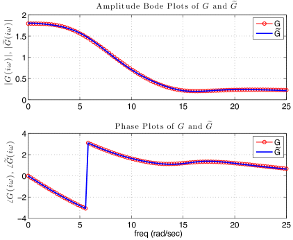
Fig. 3: Supersonic inlet flow model: amplitude and phase Bode plots of ${\mathbf{G}}(s)$ and $\widetilde{{\mathbf{G}}}(s)$.

6 Stokes-type descriptor systems of index 2

In this section, we consider a Stokes-type descriptor system of the form

$$\begin{array}[]{rcl}{\mathbf{E}}_{11}\dot{{\mathbf{x}}}_{1}(t)&=&{\mathbf{A}}_{11}{\mathbf{x}}_{1}(t)+{\mathbf{A}}_{12}{\mathbf{x}}_{2}(t)+{\mathbf{B}}_{1}{\mathbf{u}}(t),\\ \mathbf{0}&=&{\mathbf{A}}_{21}{\mathbf{x}}_{1}(t)+{\mathbf{B}}_{2}{\mathbf{u}}(t),\\ {\mathbf{y}}(t)&=&{\mathbf{C}}_{1}{\mathbf{x}}_{1}(t)+{\mathbf{C}}_{2}{\mathbf{x}}_{2}(t)+{\mathbf{D}}{\mathbf{u}}(t),\\ \end{array}$$ (36)

where the state is ${\mathbf{x}}(t)=\left[{\mathbf{x}}_{1}^{T}(t),\;{\mathbf{x}}_{2}^{T}(t)\right]^{T}\in\mbox{\Bb R}^{n}$ with ${\mathbf{x}}_{1}(t)\in\mbox{\Bb R}^{n_{1}}$, ${\mathbf{x}}_{2}(t)\in\mbox{\Bb R}^{n_{2}}$ and $n_{1}+n_{2}=n$, the input is ${\mathbf{u}}(t)\in\mbox{\Bb R}^{m}$, the output is ${\mathbf{y}}(t)\in\mbox{\Bb R}^{p}$, and ${\mathbf{E}}_{11},{\mathbf{A}}_{11}\in\mbox{\Bb R}^{n_{1}\times n_{1}}$, ${\mathbf{A}}_{12}\in\mbox{\Bb R}^{n_{1}\times n_{2}}$, ${\mathbf{A}}_{21}\in\mbox{\Bb R}^{n_{2}\times n_{1}}$, ${\mathbf{B}}_{1}\in\mbox{\Bb R}^{n_{1}\times m}$, ${\mathbf{B}}_{2}\in\mbox{\Bb R}^{n_{2}\times m}$, ${\mathbf{C}}_{1}\in\mbox{\Bb R}^{p\times n_{1}}$, ${\mathbf{C}}_{2}\in\mbox{\Bb R}^{p\times n_{2}}$, and ${\mathbf{D}}\in\mbox{\Bb R}^{p\times m}$. We assume that ${\mathbf{E}}_{11}$ is nonsingular, ${\mathbf{A}}_{12}$ and ${\mathbf{A}}_{21}^{T}$ have both full column rank and ${\mathbf{A}}_{21}{\mathbf{E}}_{11}^{-1}{\mathbf{A}}_{12}$ is nonsingular. In this case, system (36) is of index 2.

In [17], the authors showed how to apply ADI-based balanced truncation to systems of the form (36) without explicit projector computation. Here, we extend this analysis to interpolatory model reduction and show how to reduce (36) optimally in the ${{\mathcal{H}}_{2}}$-norm without computing the deflating subspaces. Unlike [17], ${\mathbf{E}}_{11}$ is not assumed to be symmetric and positive definite, and ${\mathbf{A}}_{21}$ is not assumed to be equal to ${\mathbf{A}}_{12}^{T}$.

First, consider system (36) with ${\mathbf{B}}_{2}=\mathbf{0}$, as the case of ${\mathbf{B}}_{2}\neq\mathbf{0}$ follows similarly. Following the exposition of [17], consider the projectors

$$\begin{array}[]{rcl}{\boldsymbol{\Pi}}_{l}&=&{\mathbf{I}}-{\mathbf{E}}_{11}^{-1}{\mathbf{A}}_{12}({\mathbf{A}}_{21}{\mathbf{E}}_{11}^{-1}{\mathbf{A}}_{12})^{-1}{\mathbf{A}}_{21},\\[2.84526pt] {\boldsymbol{\Pi}}_{r}&=&{\mathbf{I}}-{\mathbf{A}}_{12}({\mathbf{A}}_{21}{\mathbf{E}}_{11}^{-1}{\mathbf{A}}_{12})^{-1}{\mathbf{A}}_{21}{\mathbf{E}}_{11}^{-1}.\end{array}$$

Then the descriptor system (36) can be decoupled into a system

$$\begin{array}[]{rcl}{\boldsymbol{\Pi}}_{l}{\mathbf{E}}_{11}{\boldsymbol{\Pi}}_{r}\dot{{\mathbf{x}}}_{1}(t)&=&{\boldsymbol{\Pi}}_{l}{\mathbf{A}}_{11}{\boldsymbol{\Pi}}_{r}{\mathbf{x}}_{1}(t)+{\boldsymbol{\Pi}}_{l}{\mathbf{B}}_{1}{\mathbf{u}}(t)\\ {\mathbf{y}}(t)&=&{\mathbf{C}}{\boldsymbol{\Pi}}_{r}{\mathbf{x}}_{1}(t)+\mbox{\boldmath${\mathcal{D}}$}{\mathbf{u}}(t)\end{array}$$ (37)

with

$$\begin{array}[]{rcl}{\mathbf{C}}&=&{\mathbf{C}}_{1}-{\mathbf{C}}_{2}({\mathbf{A}}_{21}{\mathbf{E}}_{11}^{-1}{\mathbf{A}}_{12})^{-1}{\mathbf{A}}_{21}{\mathbf{E}}_{11}^{-1}{\mathbf{A}}_{11},\\[2.84526pt] \mbox{\boldmath${\mathcal{D}}$}&=&{\mathbf{D}}-{\mathbf{C}}_{2}({\mathbf{A}}_{21}{\mathbf{E}}_{11}^{-1}{\mathbf{A}}_{12})^{-1}{\mathbf{A}}_{21}{\mathbf{E}}_{11}^{-1}{\mathbf{B}}_{1},\end{array}$$

and an algebraic equation

$${\mathbf{x}}_{2}(t)=-({\mathbf{A}}_{21}{\mathbf{E}}_{11}^{-1}{\mathbf{A}}_{12})^{-1}{\mathbf{A}}_{21}{\mathbf{E}}_{11}^{-1}{\mathbf{A}}_{11}{\mathbf{x}}_{1}(t)-({\mathbf{A}}_{21}{\mathbf{E}}_{11}^{-1}{\mathbf{A}}_{12})^{-1}{\mathbf{A}}_{21}{\mathbf{E}}_{11}^{-1}{\mathbf{B}}_{1}{\mathbf{u}}(t).$$

By decomposing ${\boldsymbol{\Pi}}_{l}$ and ${\boldsymbol{\Pi}}_{r}$ as

$${\boldsymbol{\Pi}}_{l}=\mbox{\boldmath$\Theta$}_{l,1}\mbox{\boldmath$\Theta$}_{l,2}^{T},\qquad{\boldsymbol{\Pi}}_{r}=\mbox{\boldmath$\Theta$}_{r,1}\mbox{\boldmath$\Theta$}_{r,2}^{T}$$ (38)

with $\mbox{\boldmath$\Theta$}_{l,j},\mbox{\boldmath$\Theta$}_{r,j}\in\mbox{\Bb R}^{n_{1}\times(n_{1}-n_{2})}$ such that

$$\mbox{\boldmath$\Theta$}_{l,2}^{T}\mbox{\boldmath$\Theta$}_{l,1}={\mathbf{I}},\qquad\mbox{\boldmath$\Theta$}_{r,2}^{T}\mbox{\boldmath$\Theta$}_{r,1}={\mathbf{I}},$$ (39)

and defining $\tilde{{\mathbf{x}}}_{1}(t)=\mbox{\boldmath$\Theta$}_{r,2}^{T}{\mathbf{x}}_{1}(t)$, system (37) becomes

$$\begin{array}[]{rcl}\mbox{\boldmath$\Theta$}_{l,2}^{T}{\mathbf{E}}_{11}\mbox{\boldmath$\Theta$}_{r,1}\dot{\tilde{{\mathbf{x}}}}_{1}(t)&=&\mbox{\boldmath$\Theta$}_{l,2}^{T}{\mathbf{A}}_{11}\mbox{\boldmath$\Theta$}_{r,1}\tilde{{\mathbf{x}}}_{1}(t)+\mbox{\boldmath$\Theta$}_{l,2}^{T}{\mathbf{B}}_{1}{\mathbf{u}}(t)\\ {\mathbf{y}}(t)&=&{\mathbf{C}}\mbox{\boldmath$\Theta$}_{r,1}\tilde{{\mathbf{x}}}_{1}(t)+\mbox{\boldmath${\mathcal{D}}$}{\mathbf{u}}(t).\end{array}$$ (40)

Then the reduction of the descriptor system (36) is equivalent to the reduction of system (37) or (40). However, the beauty of this equivalence lies in the observation that the matrix $\mbox{\boldmath$\Theta$}_{l,2}^{T}{\mathbf{E}}_{11}\mbox{\boldmath$\Theta$}_{r,1}$ is nonsingular. Therefore, standard model reduction procedures for ODEs can be applied to system (40), and the obtained reduced-order model will approximate the descriptor system (36). It is important to emphasize that even though (37) and (40) are equivalent to (36), the ultimate goal of this section is to develop an interpolatory model reduction method that does not require the explicit computation of either the projectors ${\boldsymbol{\Pi}}_{l}$, ${\boldsymbol{\Pi}}_{r}$ or the basis matrices $\mbox{\boldmath$\Theta$}_{l,2}$, $\mbox{\boldmath$\Theta$}_{r,1}$. For this purpose, define the matrices

$$\mbox{\boldmath${\mathcal{E}}$}={\boldsymbol{\Pi}}_{l}{\mathbf{E}}_{11}{\boldsymbol{\Pi}}_{r},\qquad\mbox{\boldmath${\mathcal{A}}$}={\boldsymbol{\Pi}}_{l}{\mathbf{A}}_{11}{\boldsymbol{\Pi}}_{r},\qquad\mbox{\boldmath${\mathcal{B}}$}={\boldsymbol{\Pi}}_{l}{\mathbf{B}}_{1},\quad\mbox{\boldmath${\mathcal{C}}$}={\mathbf{C}}{\boldsymbol{\Pi}}_{r}.$$ (41)

In interpolation setting, the matrix of interest will be $\sigma\mbox{\boldmath${\mathcal{E}}$}-\mbox{\boldmath${\mathcal{A}}$}$ with $\sigma\in\mbox{\Bb C}$. Luckily, several key properties of $\mbox{\boldmath${\mathcal{E}}$}+\tau\mbox{\boldmath${\mathcal{A}}$}$, $\tau\in\mbox{\Bb C}$, were already introduced in [17]. However, we present these results in terms of $\sigma\mbox{\boldmath${\mathcal{E}}$}-\mbox{\boldmath${\mathcal{A}}$}$ instead of $\mbox{\boldmath${\mathcal{E}}$}+\tau\mbox{\boldmath${\mathcal{A}}$}$.

Lemma 7.

Let $\mbox{\boldmath$\Theta$}_{l,2}$ and $\mbox{\boldmath$\Theta$}_{r,1}$ be the matrices defined in (38) and let $\sigma\in\mbox{\Bb C}$ be such that $\sigma\mbox{\boldmath$\Theta$}_{l,2}^{T}{\mathbf{E}}_{11}\mbox{\boldmath$\Theta$}_{r,1}-\mbox{\boldmath$\Theta$}_{l,2}^{T}{\mathbf{A}}_{11}\mbox{\boldmath$\Theta$}_{r,1}$ is nonsingular. The matrix defined as

$$(\sigma\mbox{\boldmath${\mathcal{E}}$}-\mbox{\boldmath${\mathcal{A}}$})^{I}:=\mbox{\boldmath$\Theta$}_{r,1}(\sigma\mbox{\boldmath$\Theta$}_{l,2}^{T}{\mathbf{E}}_{11}\mbox{\boldmath$\Theta$}_{r,1}-\mbox{\boldmath$\Theta$}_{l,2}^{T}{\mathbf{A}}_{11}\mbox{\boldmath$\Theta$}_{r,1})^{-1}\mbox{\boldmath$\Theta$}_{l,2}^{T}$$ (42)

satisfies

$$(\sigma\mbox{\boldmath${\mathcal{E}}$}-\mbox{\boldmath${\mathcal{A}}$})^{I}(\sigma\mbox{\boldmath${\mathcal{E}}$}-\mbox{\boldmath${\mathcal{A}}$})={\boldsymbol{\Pi}}_{r}\quad\text{and}\quad(\sigma\mbox{\boldmath${\mathcal{E}}$}-\mbox{\boldmath${\mathcal{A}}$})(\sigma\mbox{\boldmath${\mathcal{E}}$}-\mbox{\boldmath${\mathcal{A}}$})^{I}={\boldsymbol{\Pi}}_{l}.$$

Similarly, the matrix defined as

$$(\sigma\mbox{\boldmath${\mathcal{E}}$}^{T}-\mbox{\boldmath${\mathcal{A}}$}^{T})^{I}:=\mbox{\boldmath$\Theta$}_{l,2}(\sigma\mbox{\boldmath$\Theta$}_{r,1}^{T}{\mathbf{E}}_{11}^{T}\mbox{\boldmath$\Theta$}_{l,2}-\mbox{\boldmath$\Theta$}_{r,1}^{T}{\mathbf{A}}_{11}^{T}\mbox{\boldmath$\Theta$}_{l,2})^{-1}\mbox{\boldmath$\Theta$}_{r,1}^{T}$$ (43)

satisfies

$$(\sigma\mbox{\boldmath${\mathcal{E}}$}^{T}-\mbox{\boldmath${\mathcal{A}}$}^{T})^{I}(\sigma\mbox{\boldmath${\mathcal{E}}$}^{T}-\mbox{\boldmath${\mathcal{A}}$}^{T})={\boldsymbol{\Pi}}_{l}^{T}\quad\text{and}\quad(\sigma\mbox{\boldmath${\mathcal{E}}$}^{T}-\mbox{\boldmath${\mathcal{A}}$}^{T})(\sigma\mbox{\boldmath${\mathcal{E}}$}^{T}-\mbox{\boldmath${\mathcal{A}}$}^{T})^{I}={\boldsymbol{\Pi}}_{r}^{T}.$$

Proof.

Following a similar argument to that in [17], the proof of the first equality follows directly from (38) and (42). Indeed, we have

$$(\sigma\mbox{\boldmath${\mathcal{E}}$}- \mbox{\boldmath${\mathcal{A}}$})^{I}(\sigma\mbox{\boldmath${\mathcal{E}}$}-\mbox{\boldmath${\mathcal{A}}$})=\mbox{\boldmath$\Theta$}_{r,1}(\sigma\mbox{\boldmath$\Theta$}_{l,2}^{T}{\mathbf{E}}_{11}\mbox{\boldmath$\Theta$}_{r,1}-\mbox{\boldmath$\Theta$}_{l,2}^{T}{\mathbf{A}}_{11}\mbox{\boldmath$\Theta$}_{r,1})^{-1}\mbox{\boldmath$\Theta$}_{l,2}^{T}{\boldsymbol{\Pi}}_{l}(\sigma{\mathbf{E}}_{11}-{\mathbf{A}}_{11}){\boldsymbol{\Pi}}_{r}$$

$$=\mbox{\boldmath$\Theta$}_{r,1}(\sigma\mbox{\boldmath$\Theta$}_{l,2}^{T}{\mathbf{E}}_{11}\mbox{\boldmath$\Theta$}_{r,1}-\mbox{\boldmath$\Theta$}_{l,2}^{T}{\mathbf{A}}_{11}\mbox{\boldmath$\Theta$}_{r,1})^{-1}\mbox{\boldmath$\Theta$}_{l,2}^{T}(\sigma{\mathbf{E}}_{11}-{\mathbf{A}}_{11})\mbox{\boldmath$\Theta$}_{r,1}\mbox{\boldmath$\Theta$}_{r,2}^{T}$$

$$=\mbox{\boldmath$\Theta$}_{r,1}\mbox{\boldmath$\Theta$}_{r,2}^{T}={\boldsymbol{\Pi}}_{r}.$$

The remaining equalities follow similarly. ∎

At first glance, the definition of the generalized inverses in (42) and (43) may seem to be irrelevant for model reduction of the descriptor system (36). Recall that reducing (36) is equivalent to reducing system (37) and the interpolatory projection method for (37) will require inverting $(\sigma\mbox{\boldmath${\mathcal{E}}$}-\mbox{\boldmath${\mathcal{A}}$})$ and $(\sigma\mbox{\boldmath${\mathcal{E}}$}^{T}-\mbox{\boldmath${\mathcal{A}}$}^{T})$. However, these inverses do not exist. As a result, definitions (42) and (43) become pivotal in order to achieve interpolatory model reduction of (37) and, thereby, of (36) as shown in the next theorem.

Theorem 8.

Let $s=\sigma,\mu\in\mbox{\Bb C}$ be such that the matrices

$$s\mbox{\boldmath$\Theta$}_{l,2}^{T}{\mathbf{E}}_{11}\mbox{\boldmath$\Theta$}_{r,1}-\mbox{\boldmath$\Theta$}_{l,2}^{T}{\mathbf{A}}_{11}\mbox{\boldmath$\Theta$}_{r,1}\qquad\mbox{and}\qquad s{\mathbf{W}}^{T}{\mathbf{E}}_{11}{\mathbf{V}}-{\mathbf{W}}^{T}{\mathbf{A}}_{11}{\mathbf{V}}$$

are invertible. Define the reduced-order model

$${\widetilde{{\mathbf{G}}}}(s) ={\mathbf{C}}{\mathbf{V}}(s{\mathbf{W}}^{T}{\mathbf{E}}_{11}{\mathbf{V}}-{\mathbf{W}}^{T}{\mathbf{A}}_{11}{\mathbf{V}})^{-1}{\mathbf{W}}^{T}{\mathbf{B}}_{1}+\mbox{\boldmath${\mathcal{D}}$}.$$ (44)

Let $\mathbf{\mathsf{b}}\in\mbox{\Bb C}^{m}$ and $\mathbf{\mathsf{c}}\in\mbox{\Bb C}^{p}$ be fixed nontrivial vectors.

1. If $(\sigma\mbox{\boldmath${\mathcal{E}}$}-\mbox{\boldmath${\mathcal{A}}$})^{I}\mbox{\boldmath${\mathcal{B}}$}\mathbf{\mathsf{b}}\in\mathrm{Im}({\mathbf{V}})\subset\mathrm{Im}(\mbox{\boldmath$\Theta$}_{r,1})$ and $(\mu\mbox{\boldmath${\mathcal{E}}$}^{T}-\mbox{\boldmath${\mathcal{A}}$}^{T})^{I}\mbox{\boldmath${\mathcal{C}}$}^{T}\mathbf{\mathsf{c}}\in\mathrm{Im}({\mathbf{W}})\subset\mathrm{Im}(\mbox{\boldmath$\Theta$}_{l,2})$, then ${{\mathbf{G}}}(\sigma)\mathbf{\mathsf{b}}={\widetilde{{\mathbf{G}}}}(\sigma)\mathbf{\mathsf{b}}$ and $\mathbf{\mathsf{c}}^{T}{{\mathbf{G}}}(\mu)=\mathbf{\mathsf{c}}^{T}{\widetilde{{\mathbf{G}}}}(\mu).$

2. If, in addition, $\sigma=\mu$, then $\mathbf{\mathsf{c}}^{T}{\mathbf{G}}^{\prime}(\sigma)\mathbf{\mathsf{b}}=\mathbf{\mathsf{c}}^{T}{\widetilde{{\mathbf{G}}}}^{\prime}(\sigma)\mathbf{\mathsf{b}}.$

Remark 6.1.

Before presenting the proof, we want to emphasize that this interpolation result is different than the usual interpolation framework given in Theorem 1, where the projection matrices ${\mathbf{V}}$ and ${\mathbf{W}}$ are constructed using ${\mathbf{A}}$, ${\mathbf{E}}$, ${\mathbf{B}}$ and ${\mathbf{C}}$ and then the projection is applied to the same quantities. In Theorem 8, however, the projection matrices ${\mathbf{V}}$ and ${\mathbf{W}}$ are constructed using the system matrices of (37), namely $\mbox{\boldmath${\mathcal{A}}$},\mbox{\boldmath${\mathcal{E}}$},\mbox{\boldmath${\mathcal{B}}$}$ and ${\mathcal{C}}$. But then the projection (model reduction) is applied to the system matrices of (36), namely ${\mathbf{E}}_{11},{\mathbf{A}}_{11},{\mathbf{B}}_{1}$ and ${\mathbf{C}}$. Thus, the proof will serve to fill in this important gap.

Proof.

Since systems (36) and (40) are equivalent, they have the same transfer function given by

$${{\mathbf{G}}}(s)={\mathbf{C}}\mbox{\boldmath$\Theta$}_{r,1}(s\mbox{\boldmath$\Theta$}_{l,2}^{T}{\mathbf{E}}_{11}\mbox{\boldmath$\Theta$}_{r,1}-\mbox{\boldmath$\Theta$}_{l,2}^{T}{\mathbf{A}}_{11}\mbox{\boldmath$\Theta$}_{r,1})^{-1}\mbox{\boldmath$\Theta$}_{l,2}^{T}{\mathbf{B}}_{1}+\mbox{\boldmath${\mathcal{D}}$}.$$

Since $\mbox{\boldmath$\Theta$}_{l,2}^{T}{\mathbf{E}}_{11}\mbox{\boldmath$\Theta$}_{r,1}$ in (40) is nonsingular, we make use of Theorem 1. Define $\widetilde{{\mathbf{V}}}$ and $\widetilde{{\mathbf{W}}}$ such that

$${\mathbf{V}}=\mbox{\boldmath$\Theta$}_{r,1}\widetilde{\mathbf{V}}\qquad\text{and}\qquad{\mathbf{W}}=\mbox{\boldmath$\Theta$}_{l,2}\widetilde{\mathbf{W}}.$$ (45)

Pluging these matrices into (44), we obtain that

$$\widetilde{{\mathbf{G}}}(s)={\mathbf{C}}\mbox{\boldmath$\Theta$}_{r,1}\widetilde{\mathbf{V}}(s\widetilde{\mathbf{W}}^{T}\mbox{\boldmath$\Theta$}_{l,2}^{T}{\mathbf{E}}_{11}\mbox{\boldmath$\Theta$}_{r,1}\widetilde{\mathbf{V}}-\widetilde{\mathbf{W}}^{T}\mbox{\boldmath$\Theta$}_{l,2}^{T}{\mathbf{A}}_{11}\mbox{\boldmath$\Theta$}_{r,1}\widetilde{\mathbf{V}})^{-1}\widetilde{\mathbf{W}}^{T}\mbox{\boldmath$\Theta$}_{l,2}^{T}{\mathbf{B}}_{1}+\mbox{\boldmath${\mathcal{D}}$}.$$

Moreover, it follows from (39) that $\widetilde{\mathbf{V}}=\mbox{\boldmath$\Theta$}_{r,2}^{T}{\mathbf{V}}$ and $\widetilde{\mathbf{W}}=\mbox{\boldmath$\Theta$}_{l,1}^{T}{\mathbf{W}}$. To prove the first claim in part $1$, we note that (38) implies that

$$\mbox{\boldmath$\Theta$}_{l,2}^{T}\mbox{\boldmath${\mathcal{B}}$}=\mbox{\boldmath$\Theta$}_{l,2}^{T}{\boldsymbol{\Pi}}_{l}{\mathbf{B}}_{1}=\mbox{\boldmath$\Theta$}_{l,2}^{T}\mbox{\boldmath$\Theta$}_{l,1}\mbox{\boldmath$\Theta$}_{l,2}^{T}{\mathbf{B}}_{1}=\mbox{\boldmath$\Theta$}_{l,2}^{T}{\mathbf{B}}_{1}.$$ (46)

Since $(\sigma\mbox{\boldmath${\mathcal{E}}$}-\mbox{\boldmath${\mathcal{A}}$})^{I}\mbox{\boldmath${\mathcal{B}}$}\mathbf{\mathsf{b}}\in\mathrm{Im}({\mathbf{V}})$, there exists ${\mathbf{q}}\in\mbox{\Bb R}^{r}$ such that $(\sigma\mbox{\boldmath${\mathcal{E}}$}-\mbox{\boldmath${\mathcal{A}}$})^{I}\mbox{\boldmath${\mathcal{B}}$}\mathbf{\mathsf{b}}={\mathbf{V}}{\mathbf{q}}$. Using (42) (45) and (46), this equation can be written as

$$\mbox{\boldmath$\Theta$}_{r,1}(\sigma\mbox{\boldmath$\Theta$}_{l,2}^{T}{\mathbf{E}}_{11}\mbox{\boldmath$\Theta$}_{r,1}-\mbox{\boldmath$\Theta$}_{l,2}^{T}{\mathbf{A}}_{11}\mbox{\boldmath$\Theta$}_{r,1})^{-1}\mbox{\boldmath$\Theta$}_{l,2}^{T}{\mathbf{B}}_{1}{\mathbf{b}}=\mbox{\boldmath$\Theta$}_{r,1}\widetilde{\mathbf{V}}{\mathbf{q}}.$$

The left multiplication by $\mbox{\boldmath$\Theta$}_{r,2}^{T}$ gives

$$(\sigma\mbox{\boldmath$\Theta$}_{l,2}^{T}{\mathbf{E}}_{11}\mbox{\boldmath$\Theta$}_{r,1}-\mbox{\boldmath$\Theta$}_{l,2}^{T}{\mathbf{A}}_{11}\mbox{\boldmath$\Theta$}_{r,1})^{-1}\mbox{\boldmath$\Theta$}_{l,2}^{T}{\mathbf{B}}_{1}\mathbf{\mathsf{b}}=\widetilde{\mathbf{V}}{\mathbf{q}}.$$

Hence, $(\sigma\mbox{\boldmath$\Theta$}_{l,2}^{T}{\mathbf{E}}_{11}\mbox{\boldmath$\Theta$}_{r,1}-\mbox{\boldmath$\Theta$}_{l,2}^{T}{\mathbf{A}}_{11}\mbox{\boldmath$\Theta$}_{r,1})^{-1}\mbox{\boldmath$\Theta$}_{l,2}^{T}{\mathbf{B}}_{1}\mathbf{\mathsf{b}}\in\mathrm{Im}(\widetilde{\mathbf{V}})$. Then it follows from Theorem 1 that ${{\mathbf{G}}}(\sigma)\mathbf{\mathsf{b}}=\widetilde{{\mathbf{G}}}(\sigma)\mathbf{\mathsf{b}}$. The equation $\mathbf{\mathsf{c}}^{T}{\mathbf{G}}(\sigma)=\mathbf{\mathsf{c}}^{T}\widetilde{{\mathbf{G}}}(\sigma)$ can be obtained similarly. The proof of part $2$ follows from part $3$ of Theorem 1. ∎

It should be noted that the conditions $\mathrm{Im}({\mathbf{V}})\subset\mathrm{Im}(\mbox{\boldmath$\Theta$}_{r,1})$ and $\mathrm{Im}({\mathbf{W}})\subset\mathrm{Im}(\mbox{\boldmath$\Theta$}_{l,2})$ in part 1 of Theorem 8 are automatically fulfilled if for given interpolation points $\{\sigma_{i}\}_{i=1}^{r}$, $\{\mu_{i}\}_{i=1}^{r}$ and tangential directions $\{\mathbf{\mathsf{b}}_{i}\}_{i=1}^{r}$, $\{\mathbf{\mathsf{c}}_{i}\}_{i=1}^{r}$, we choose

$$\begin{array}[]{rcl}\mathrm{Im}({\mathbf{V}})&=&\mathrm{span}\{(\sigma_{1}\mbox{\boldmath${\mathcal{E}}$}-\mbox{\boldmath${\mathcal{A}}$})^{I}\mbox{\boldmath${\mathcal{B}}$}\mathbf{\mathsf{b}}_{1},\ldots,(\sigma_{r}\mbox{\boldmath${\mathcal{E}}$}-\mbox{\boldmath${\mathcal{A}}$})^{I}\mbox{\boldmath${\mathcal{B}}$}\mathbf{\mathsf{b}}_{r}\},\\ \mathrm{Im}({\mathbf{W}})&=&\mathrm{span}\{(\mu_{1}\mbox{\boldmath${\mathcal{E}}$}^{T}-\mbox{\boldmath${\mathcal{A}}$}^{T})^{I}\mbox{\boldmath${\mathcal{C}}$}^{T}\mathbf{\mathsf{c}}_{1},\ldots,(\sigma_{r}\mbox{\boldmath${\mathcal{E}}$}^{T}-\mbox{\boldmath${\mathcal{A}}$}^{T})^{I}\mbox{\boldmath${\mathcal{C}}$}^{T}\mathbf{\mathsf{c}}_{r}\}.\end{array}$$

6.1 Computational issues related to the reduction of index-2 descriptor systems

Even though Theorem 8 shows how to enforce interpolation for the descriptor system (36), the spectral projectors are still implicitly hidden in the definitions of $(\sigma\mbox{\boldmath${\mathcal{E}}$}-\mbox{\boldmath${\mathcal{A}}$})^{I}$ and $(\sigma\mbox{\boldmath${\mathcal{E}}$}^{T}-\mbox{\boldmath${\mathcal{A}}$}^{T})^{I}$. It has been shown in [17] how to compute the matrix-vector product $(\mbox{\boldmath${\mathcal{E}}$}+\tau\mbox{\boldmath${\mathcal{A}}$})^{I}{\mathbf{f}}$ for a given vector ${\mathbf{f}}$ without explicitly forming $(\mbox{\boldmath${\mathcal{E}}$}+\tau\mbox{\boldmath${\mathcal{A}}$})^{I}$. This approach can also be used in interpolatory model reduction, where the quantities of interest are $(\sigma\mbox{\boldmath${\mathcal{E}}$}-\mbox{\boldmath${\mathcal{A}}$})^{I}\mbox{\boldmath${\mathcal{B}}$}\mathbf{\mathsf{b}}$ and $(\mu\mbox{\boldmath${\mathcal{E}}$}^{T}-\mbox{\boldmath${\mathcal{A}}$}^{T})^{I}\mbox{\boldmath${\mathcal{C}}$}^{T}\mathbf{\mathsf{c}}$. The proof of the following result is analogous to those in [17], and, therefore, it is omitted.

Lemma 9.

Let $s=\sigma,\mu$ be such that $s\mbox{\boldmath$\Theta$}_{l,2}^{T}{\mathbf{E}}_{11}\mbox{\boldmath$\Theta$}_{r,1}-\mbox{\boldmath$\Theta$}_{l,2}^{T}{\mathbf{A}}_{11}\mbox{\boldmath$\Theta$}_{r,1}$ is invertible. Then the vector

$${\mathbf{v}}=(\sigma\mbox{\boldmath${\mathcal{E}}$}-\mbox{\boldmath${\mathcal{A}}$})^{I}\mbox{\boldmath${\mathcal{B}}$}\mathbf{\mathsf{b}}$$ (47)

solves

$$\left[\begin{array}[]{cc}\sigma{\mathbf{E}}_{11}-{\mathbf{A}}_{11}&{\mathbf{A}}_{12}\\ {\mathbf{A}}_{21}&\mathbf{0}\end{array}\right]\left[\begin{array}[]{cc}{\mathbf{v}}\\ {\mathbf{z}}\end{array}\right]=\left[\begin{array}[]{cc}{\mathbf{B}}_{1}\mathbf{\mathsf{b}}\\ \mathbf{0}\end{array}\right],$$ (54)

and the vector

$${\mathbf{w}}=(\mu\mbox{\boldmath${\mathcal{E}}$}^{T}-\mbox{\boldmath${\mathcal{A}}$}^{T})^{I}\mbox{\boldmath${\mathcal{C}}$}^{T}\mathbf{\mathsf{c}}$$ (55)

solves

$$\left[\begin{array}[]{cc}\mu{\mathbf{E}}_{11}^{T}-{\mathbf{A}}_{11}^{T}&{\mathbf{A}}_{21}^{T}\\ {\mathbf{A}}_{12}^{T}&\mathbf{0}\end{array}\right]\left[\begin{array}[]{cc}{\mathbf{w}}\\ {\mathbf{q}}\end{array}\right]=\left[\begin{array}[]{cc}{\mathbf{C}}^{T}\mathbf{\mathsf{c}}\\ \mathbf{0}\end{array}\right].$$ (62)

From a computational perspective of implementing Theorem 8, the importance of this result is clear. To achieve interpolation, Theorem 8 relies on computing the quantities $(\sigma\mbox{\boldmath${\mathcal{E}}$}-\mbox{\boldmath${\mathcal{A}}$})^{I}\mbox{\boldmath${\mathcal{B}}$}\mathbf{\mathsf{b}}$ and $(\sigma\mbox{\boldmath${\mathcal{E}}$}^{T}-\mbox{\boldmath${\mathcal{A}}$}^{T})^{I}\mbox{\boldmath${\mathcal{C}}$}^{T}\mathbf{\mathsf{c}},$ both of which involve the computation of $\mbox{\boldmath$\Theta$}_{l,2}$ and $\mbox{\boldmath$\Theta$}_{r,1}$. However, Lemma 9 illustrates that the computation of these basis matrices is unnecessary and only the linear systems (54) and (62) need to be solved. This observation leads to Algorithm 6.1 below for interpolatory model reduction of Stokes-type descriptor systems of index 2.

Algorithm 6.1.

Interpolatory model reduction for Stokes-type
                         descriptor systems of index 2 1) Make an initial selection of the interpolation points $\{\sigma_{i}\}_{i=1}^{r}$ and the tangent directions $\{{\mathbf{\mathsf{b}}}_{i}\}_{i=1}^{r}$ and $\{{\mathbf{\mathsf{c}}}_{i}\}_{i=1}^{r}$. 2) For $i=1,\ldots,r$, solve $$\left[\begin{array}[]{cc}\sigma_{i}{\mathbf{E}}_{11}-{\mathbf{A}}_{11}&{\mathbf{A}}_{12}\\ {\mathbf{A}}_{21}&\mathbf{0}\end{array}\right]\left[\begin{array}[]{cc}{\mathbf{v}}_{i}\\ {\mathbf{z}}\end{array}\right]=\left[\begin{array}[]{cc}{\mathbf{B}}_{1}\mathbf{\mathsf{b}}_{i}\\ \mathbf{0}\end{array}\right],$$ $$\left[\begin{array}[]{cc}\sigma_{i}{\mathbf{E}}_{11}^{T}-{\mathbf{A}}_{11}^{T}&{\mathbf{A}}_{21}^{T}\\ {\mathbf{A}}_{12}^{T}&\mathbf{0}\end{array}\right]\left[\begin{array}[]{cc}{\mathbf{w}}_{i}\\ {\mathbf{q}}\end{array}\right]=\left[\begin{array}[]{cc}{\mathbf{C}}^{T}\mathbf{\mathsf{c}}_{i}\\ \mathbf{0}\end{array}\right].$$ 3) ${\mathbf{V}}=\left[{\mathbf{v}}_{1},\dots,{\mathbf{v}}_{r}\right]$,  ${\mathbf{W}}=\left[{\mathbf{w}}_{1},\dots,{\mathbf{w}}_{r}\right]$. 4) ${\widetilde{{\mathbf{E}}}}={\mathbf{W}}^{T}{\mathbf{E}}_{11}{\mathbf{V}}$, ${\widetilde{{\mathbf{A}}}}={\mathbf{W}}^{T}{\mathbf{A}}_{11}{\mathbf{V}}$, ${\widetilde{{\mathbf{B}}}}={\mathbf{W}}^{T}{\mathbf{B}}_{1}$, ${\widetilde{{\mathbf{C}}}}={\mathbf{C}}{\mathbf{V}}$, ${\widetilde{{\mathbf{D}}}}=\mbox{\boldmath${\mathcal{D}}$}.$

Once a computationally effective bi-tangential Hermite interpolation framework is established for index-2 descriptor systems, extending it to optimal ${{\mathcal{H}}_{2}}$ model reduction via IRKA is straightforward and given in Algorithm 6.2. It follows from the structure of this algorithm that upon convergence the reduced model ${\widetilde{{\mathbf{G}}}}(s)={\widetilde{{\mathbf{C}}}}(s{\widetilde{{\mathbf{E}}}}\!-\!{\widetilde{{\mathbf{A}}}})^{-1}{\widetilde{{\mathbf{B}}}}\!+\!\widetilde{{\mathbf{D}}}$ satisfies the first-order conditions for ${{\mathcal{H}}_{2}}$ optimality.

Algorithm 6.2.

IRKA for Stokes-type descriptor system of index 2 1) Make an initial shift selection $\{\sigma_{i}\}_{i=1}^{r}$ and initial tangent directions $\{{\mathbf{\mathsf{b}}}_{i}\}_{i=1}^{r}$ and $\{{\mathbf{\mathsf{c}}}_{i}\}_{i=1}^{r}$. 2) Apply Algorithm 6.1 to obtain ${\widetilde{{\mathbf{E}}}}$, ${\widetilde{{\mathbf{A}}}}$, ${\widetilde{{\mathbf{B}}}}$, ${\widetilde{{\mathbf{C}}}}$ and ${\widetilde{{\mathbf{D}}}}$. 3) while (not converged) a) Compute ${\mathbf{Y}}^{*}{\widetilde{{\mathbf{A}}}}{\mathbf{Z}}=diag(\lambda_{1},\ldots,\lambda_{r})$ and ${\mathbf{Y}}^{*}{\widetilde{{\mathbf{E}}}}{\mathbf{Z}}={\mathbf{I}}$, where the columns of ${\mathbf{Z}}=[{\mathbf{z}}_{1},\ldots,{\mathbf{z}}_{r}]$ and ${\mathbf{Y}}=[{\mathbf{y}}_{1},\ldots,{\mathbf{y}}_{r}]$ are, respectively, the right and left eigenvectors of $\lambda{\widetilde{{\mathbf{E}}}}-{\widetilde{{\mathbf{A}}}}$. b) $\sigma_{i}\leftarrow-\lambda_{i}$, ${\mathbf{\mathsf{b}}}_{i}^{T}\leftarrow{\mathbf{y}}_{i}^{*}{\widetilde{{\mathbf{B}}}}$ and ${\mathbf{\mathsf{c}}}_{i}\leftarrow{\widetilde{{\mathbf{C}}}}{\mathbf{z}}_{i}$ for $i=1,\ldots,r$. c) Apply Algorithm 6.1 to obtain ${\widetilde{{\mathbf{E}}}}$, ${\widetilde{{\mathbf{A}}}}$, ${\widetilde{{\mathbf{B}}}}$, ${\widetilde{{\mathbf{C}}}}$ and ${\widetilde{{\mathbf{D}}}}$. end while

Remark 6.2.

As shown in [17], the general case ${\mathbf{B}}_{2}\neq\mathbf{0}$ can be handled similar to the case ${\mathbf{B}}_{2}=\mathbf{0}$. First note that the state ${\mathbf{x}}_{1}(t)$ can be decomposed as ${\mathbf{x}}_{1}(t)={\mathbf{x}}_{0}(t)+{\mathbf{x}}_{g}(t)$, where ${\mathbf{x}}_{g}(t)=-{\mathbf{E}}_{11}^{-1}{\mathbf{A}}_{12}({\mathbf{A}}_{21}{\mathbf{E}}_{11}^{-1}{\mathbf{A}}_{12})^{-1}{\mathbf{B}}_{2}{\mathbf{u}}(t)$ and ${\mathbf{x}}_{0}(t)$ satisfies ${\mathbf{A}}_{21}{\mathbf{x}}_{0}(t)=0$. After some algebraic manipulations, this leads to

$$\begin{array}[]{rcl}{\boldsymbol{\Pi}}_{l}{\mathbf{E}}_{11}{\boldsymbol{\Pi}}_{r}\dot{{\mathbf{x}}}_{0}(t)&=&{\boldsymbol{\Pi}}_{l}{\mathbf{A}}_{11}{\boldsymbol{\Pi}}_{r}{\mathbf{x}}_{0}(t)+{\boldsymbol{\Pi}}_{l}{\mathbf{B}}{\mathbf{u}}(t),\\ {\mathbf{y}}(t)&=&{\mathbf{C}}{\boldsymbol{\Pi}}_{r}{\mathbf{x}}_{0}(t)+\mbox{\boldmath${\mathcal{D}}$}{\mathbf{u}}(t)-{\mathbf{C}}_{2}({\mathbf{A}}_{21}{\mathbf{E}}_{11}^{-1}{\mathbf{A}}_{12})^{-1}{\mathbf{B}}_{2}\dot{{\mathbf{u}}}(t),\\ \end{array}$$ (63)

where

$${\mathbf{C}}={\mathbf{C}}_{1}-{\mathbf{C}}_{2}({\mathbf{A}}_{21}{\mathbf{E}}_{11}^{-1}{\mathbf{A}}_{12})^{-1}{\mathbf{A}}_{21}{\mathbf{E}}_{11}^{-1}{\mathbf{A}}_{11},$$ (64)

$${\mathbf{B}}={\mathbf{B}}_{1}-{\mathbf{A}}_{11}{\mathbf{E}}_{11}^{-1}{\mathbf{A}}_{12}({\mathbf{A}}_{21}{\mathbf{E}}_{11}^{-1}{\mathbf{A}}_{12})^{-1}{\mathbf{B}}_{2},$$ (65)

$$\mbox{\boldmath${\mathcal{D}}$}={\mathbf{D}}-{\mathbf{C}}_{2}({\mathbf{A}}_{21}{\mathbf{E}}_{11}^{-1}{\mathbf{A}}_{12})^{-1}{\mathbf{A}}_{21}{\mathbf{E}}_{11}^{-1}{\mathbf{B}}_{1}.$$ (66)

Therefore, the ${\mathbf{B}}_{2}\neq 0$ case extends to the interpolation framework as well by defining

$$\widehat{\mbox{\boldmath${\mathcal{E}}$}}={\boldsymbol{\Pi}}_{l}{\mathbf{E}}_{11}{\boldsymbol{\Pi}}_{r},\quad\widehat{\mbox{\boldmath${\mathcal{A}}$}}={\boldsymbol{\Pi}}_{l}{\mathbf{A}}_{11}{\boldsymbol{\Pi}}_{r},\quad\widehat{\mbox{\boldmath${\mathcal{B}}$}}={\boldsymbol{\Pi}}_{l}{\mathbf{B}},\quad\widehat{\mbox{\boldmath${\mathcal{C}}$}}={\mathbf{C}}{\boldsymbol{\Pi}}_{r}$$

and applying Theorem 8 with $\widehat{\mbox{\boldmath${\mathcal{E}}$}}$, $\widehat{\mbox{\boldmath${\mathcal{A}}$}}$, $\widehat{\mbox{\boldmath${\mathcal{B}}$}}$, $\widehat{\mbox{\boldmath${\mathcal{C}}$}}$ and $\widehat{\mbox{\boldmath${\mathcal{D}}$}}=\mbox{\boldmath${\mathcal{D}}$}-s{\mathbf{C}}_{2}({\mathbf{A}}_{21}{\mathbf{E}}_{11}^{-1}{\mathbf{A}}_{12})^{-1}{\mathbf{B}}_{2}$ instead of ${\mathcal{E}}$, ${\mathcal{A}}$, ${\mathcal{B}}$, ${\mathcal{C}}$ and ${\mathcal{D}}$.

6.2 Numerical results for Oseen equations

The model borrowed from [17] is obtained by discretizing the Oseen equations and describe the flow of a viscous and incompressible fluid in a domain $\Omega\in\mbox{\Bb R}^{2}$ representing a channel with a backward facing step. A spatial discretization using the finite element method leads to the index-$2$ descriptor system (36) with ${\mathbf{E}}_{11},{\mathbf{A}}_{11}\in\mbox{\Bb R}^{5520\times 5520}$, ${\mathbf{A}}_{12},{\mathbf{A}}_{21}^{T}\in\mbox{\Bb R}^{5520\times 761}$, ${\mathbf{B}}_{1}\in\mbox{\Bb R}^{5520\times 6}$, ${\mathbf{B}}_{2}\in\mbox{\Bb R}^{761\times 6}$, ${\mathbf{C}}_{1}\in\mbox{\Bb R}^{2\times 5520}$, ${\mathbf{C}}_{2}\in\mbox{\Bb R}^{2\times 761}$, ${\mathbf{D}}=0$, see [17] for more details on the model. Note that ${\mathbf{B}}_{2}\neq 0$ and the transfer function grows unbounded around $s=\infty$.

We approximate this system by a model of order $r=20$ using the balanced truncation method as described in [17] and the ${{\mathcal{H}}_{2}}$ optimal model reduction method given in Algorithm 6.2. The amplitude Bode plots of the full model and two reduced-order models depicted in Figure 4 clearly illustrate that interpolation-based Algorithm 6.2 leads to a high-fidelity reduced model replicating the full-order transfer function with almost no loss of accuracy and matching the performance of the balanced truncation method. The accuracy of this interpolation-based method is due to the fact that we do not choose the interpolation points in an ad hoc fashion; instead Algorithm 6.2 iteratively leads to ${{\mathcal{H}}_{2}}$ optimal interpolation points. As the difficulty in computing ${{\mathcal{H}}_{2}}$ norm of the error is clear, we approximately compute the relative ${{\mathcal{H}}_{\infty}}$-error $\frac{\|{\mathbf{G}}_{\rm sp}-\tilde{{\mathbf{G}}}_{\rm sp}\|_{\mathcal{H}_{\infty}}}{\|{\mathbf{G}}_{\rm sp}\|_{\mathcal{H}_{\infty}}}$ for both reduced-order models by sampling the imaginary axis. These errors for the balanced truncation method and Algorithm 6.2 are, respectively, $3.3284\times 10^{-6}$ and $8.9663\times 10^{-6}$. Both reduced-order models are highly accurate. It is expected that the ${{\mathcal{H}}_{\infty}}$-error in balanced truncation will be smaller than that in IRKA. While our method tries to minimize the ${{\mathcal{H}}_{2}}$-norm, the balanced truncation method is tailored towards reducing the ${{\mathcal{H}}_{\infty}}$-norm. Indeed, these numbers are further signs for the success of the interpolatory-based model reduction method as it produces a very accurate model, almost matching the accuracy of the balanced truncation approach. These observations are similar to those on IRKA whose ${{\mathcal{H}}_{\infty}}$-norm behavior was close to or even better in some cases than that of balanced truncation [1, 15].

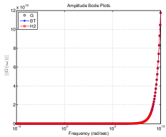
Fig. 4: Oseen equation: amplitude Bode plots of the full and reduced models

To further illustrate the accuracy in the reduced-order model computed by Algorithm 6.2, we display the time domain response plots resulting from two different input selections. In the left pane of Figure 5, we plot the outputs for the input selections ${\mathbf{u}}_{i}(t)=\text{sin}(6it)$ for $i=1,\ldots,6$ (recall that the system has $6$ inputs). The figure illustrate a perfect match between the outputs of the full and reduced-order systems. Error in the outputs for the same input selection is given in the right pane of Figure 5. Note the difference in the scale of the error plot compared to the actual output; the error is four orders of magnitude smaller. We repeat the same experiments with ${{\mathbf{u}}}_{i}(t)=\text{sin}(it)$ for $i=1,\ldots,6$ and reach the same conclusions as shown in Figure 6.

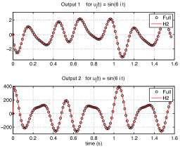
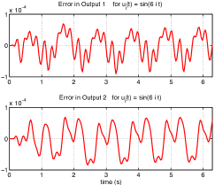
Fig. 5: Oseen equation: (left) time domain response for ${{\mathbf{u}}}_{i}(t)=\sin(6it)$; (right) error in time domain response for ${{\mathbf{u}}}_{i}(t)=\sin(6it)$.

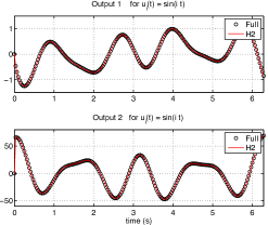
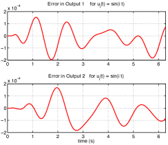
Fig. 6: Oseen equation: (left) time domain response for ${\mathbf{u}}_{i}(t)=\sin(it)$; (right) error in time domain response for ${\mathbf{u}}_{i}(t)=\sin(it)$.

7 Conclusions

For interpolatory model reduction of descriptor systems, we have introduced subspace conditions that not only guarantee interpolation conditions but also automatically enforce matching the polynomial part of the transfer function, thus preventing the error grow unbounded. We have also extended the optimal ${{\mathcal{H}}_{2}}$ interpolation point selection strategy to descriptor systems. For the index-$1$ and index-$2$ descriptor systems, we have shown how to construct the reduced-order models without computing the deflating subspaces corresponding to the finite and infinite eigenvalues explicitly. Several numerical examples have supported the theoretical discussion.

8 Acknowledgements

The authors thank Prof. M. Heinkenschloss for providing the data and the MATLAB files for the numerical example of Section 6.2. The work of S. Gugercin was supported in part by NSF through Grant DMS-0645347. The work of T. Stykel was supported in part by the Research Network FROPT: Model Reduction Based Optimal Control for Field-Flow Fractionation  funded by the German Federal Ministry of Education and Science (BMBF), Grant 05M10WAB.