Distribution of the least-squares estimators of a single Brownian trajectory diffusion coefficient

Abstract

In this paper we study the distribution function $P(u_{\alpha})$ of the estimators $u_{\alpha}\sim T^{-1}\int^{T}_{0}\,\omega(t)\,{\bf B}^{2}_{t}\,dt$, which optimise the least-squares fitting of the diffusion coefficient $D_{f}$ of a single $d$-dimensional Brownian trajectory ${\bf B}_{t}$. We pursue here the optimisation further by considering a family of weight functions of the form $\omega(t)=(t_{0}+t)^{-\alpha}$, where $t_{0}$ is a time lag and $\alpha$ is an arbitrary real number, and seeking such values of $\alpha$ for which the estimators most efficiently filter out the fluctuations. We calculate $P(u_{\alpha})$ exactly for arbitrary $\alpha$ and arbitrary spatial dimension $d$, and show that only for $\alpha=2$ the distribution $P(u_{\alpha})$ converges, as $\epsilon=t_{0}/T\to 0$, to the Dirac delta-function centered at the ensemble average value of the estimator. This allows us to conclude that only the estimators with $\alpha=2$ possess an ergodic property, so that the ensemble averaged diffusion coefficient can be obtained with any necessary precision from a single trajectory data, but at the expense of a progressively higher experimental resolution. For any $\alpha\neq 2$ the distribution attains, as $\epsilon\to 0$, a certain limiting form with a finite variance, which signifies that such estimators are not ergodic.

Keywords: diffusion and diffusion coefficient, single particle trajectory, trajectory-to-trajectory fluctuations, weighted least-squares estimators

1 Introduction

Single particle tracking (SPT) is an increasingly used method of analysis in biological and sot matter systems where the trajectories of individual particles can be optically observed. Recent advances in image processing, data storage and microscopy have led to an increasing number of papers, notably in biophysics, on single particle tracking in biological settings such as the cellular interior and the cell membrane. However the basic method of SPT owes its origin to the work of Perrin on Brownian motion [1], where optical observation is used to generate the time series for the position of an individual particle trajectory ${\bf B}_{t}$ in a medium (see, e.g., Refs. [2, 3]). Complemented by the appropriate theoretical analysis, the information drawn from a single, or a finite number of trajectories, provides insight into the underlying physical mechanisms governing the transport properties of the particles. Via the analysis of the stochastic processes manifested in single particle trajectories, SPT is routinely used for the microscopic characterisation of the thermodynamic rheological properties of complex media [4], and also to identify non-equilibrium biological effects, for example the motion of biomolecular motors [5]. In biological cells and complex fluids, SPT methods have become instrumental in demonstrating deviations from normal Brownian motion of passively moving particles (see, e.g., Refs.[6, 7, 8, 9, 10]). The method is thus potentially a powerful tool to probe physical and biological processes at the level of a single molecule [11].

The reliability of the information drawn from SPT analysis, obtained at high temporal and spatial resolution but at expense of statistical sample size is not always clear. Time averaged quantities associated with a given trajectory may be subject to large trajectory-to-trajectory fluctuations. For a wide class of anomalous diffusions, described by continuous-time random walks, time-averages of certain particle’s observables are, by their very nature, themselves random variables distinct from their ensemble averages [12, 13]. For example, the square displacement time-averaged along a given trajectory differs from the ensemble averaged mean squared displacement[13, 14, 15]. By analyzing time-averaged displacements of a particular trajectory realization, subdiffusive motion can actually look normal, although with strongly differing diffusion coefficients from one trajectory to another [13, 14, 15] and show pronounced ageing effects [16].

Standard Brownian motion is a much simpler random process than anomalous diffusion, however the analysis of its trajectories is far from being as straightforward as one might think, and all the above mentioned troublesome problems exist for Brownian motion as well. Even in bounded systems, substantial manifestations of trajectory-to-trajectory fluctuations in first passage time phenomena have been revealed [17, 18]. If one is interested in determining the diffusion coefficient of a given particle, standard fitting procedures applied to finite albeit very long trajectories unavoidably lead to fluctuating estimates $D_{f}$ of the diffusion coefficient, which might be very different from the true ensemble average value $D$, defined in a standard fashion as

$$D=\frac{\mathbb{E}\left\{{\bf B}^{2}_{t}\right\}}{2dt}\,,$$ (1.1)

where the symbol $\mathbb{E}\{\ldots\}$ denotes the ensemble average and $d$ is the spatial dimension.

To get a rough idea of how basic estimators for diffusion constants can fluctuate, consider a simple-minded, rough estimate of $D_{f}$, defining it as the slope of the line connecting the starting and the end-points ${\bf B}_{t}$ of a given trajectory, i.e., like $D$ in Eq. (1.1) but without averaging, that is $D_{f}={\bf B}^{2}_{t}/2dt$. A single trajectory diffusion coefficient $D_{f}$ so defined is a random variable whose probability density function (pdf) $P(D_{f})$ is the so-called chi-squared distribution with $d$ degrees of freedom:

$$P(D_{f})=\frac{1}{\Gamma(d/2)}\,\left(\frac{d}{2D}\right)^{d/2}\,D_{f}^{d/2-1}\,\exp\left(-\frac{d}{2}\cdot\frac{D_{f}}{D}\right)\,,$$ (1.2)

where $\Gamma(\cdot)$ is the Gamma-function. The pdf in the latter equation diverges as $D_{f}\to 0$ for $d=1$, $P(D_{f}=0)$ is constant for $d=2$, and only for $d>2$ the distribution has a bell-shaped form with the most probable value $D_{f}^{*}=(1-2/d)D$. This means that, e.g., for $d=3$, it is most likely that extracting $D_{f}$ from a single Brownian trajectory using this simple-minded approach we will obtain just one third of the true diffusion coefficient $D$.

As a matter of fact, even taking advantage of more sophisticated fitting procedures, variations by orders of magnitude have been observed in SPT measurements of the diffusion coefficient for diffusion of the LacI repressor protein along elongated DNA [19], in the plasma membrane [3] or for diffusion of a single protein in the cytoplasm and nucleoplasm of mammalian cells [20]. Such a broad dispersion of the values of the diffusion coefficient extracted from SPT measurements raises important questions about the optimal methodology, much more robust than the rough estimate mentioned above, that should be used to determine the true ensemble average value of $D$ from just a single trajectory. Clearly, it is highly desirable to have a reliable estimator even for the hypothetical pure cases, such as, e.g., unconstrained standard Brownian motion. A reliable estimator must possess an ergodic property so that its most probable value should converge to the ensemble average one and the variance should vanish as the observation time increases. This is often not the case and moreover, ergodicity of a given estimator is not known a priori and has to be tested for each particular form of the estimator. On the other hand, knowledge of the distribution of such an estimator could provide a useful gauge to identify effects of the medium complexity as opposed to variations in the underlying thermal noise driving microscopic diffusion. Recently, much effort has been invested in the analysis of this challenging problem and several important results have been obtained for the estimators based on the time-averaged mean-square displacement [22, 23, 24], mean maximal excursion [25] or the maximum likelihood approximation and its ramifications [26, 27, 28, 29, 30].

Let us define the dimensionless estimator of the diffusion coefficient as $u\equiv D_{f}/D$. In this paper, following our succinct presentation in [31], we focus on a family of least-squares estimators $u_{\alpha}$ given by

$$u_{\alpha}=\frac{A_{\alpha}}{T}\int^{T}_{0}\,\omega(t)\,{\bf B}^{2}_{t}\,dt,$$ (1.3)

where $\omega(t)$ is the weight function of the form

$$\omega(t)=\frac{1}{(t_{0}+t)^{\alpha}}\,,$$ (1.4)

$\alpha$ being a tunable exponent, (positive or negative), $t_{0}$ - a lag time and $A_{\alpha}$ - the normalisation constant, appropriately chosen such that $\mathbb{E}\left\{u_{\alpha}\right\}\equiv 1$. Therefore

$$A_{\alpha}=\frac{T}{2dD}\left(\int^{T}_{0}\frac{t\,dt}{(t_{0}+t)^{\alpha}}\right)^{-1}\,.$$ (1.5)

Note that such a normalisation permits a direct comparison of the effectiveness of estimators corresponding to different values of $\alpha$. Our goal here is to find such $\alpha$ for which $u_{\alpha}$ is ergodic, namely, so that the single trajectory diffusion coefficient $D_{f}\to D$ (or $u_{\alpha}\rightarrow 1$) as $\epsilon=t_{0}/T\to 0$.

It should be emphasised that, as a matter of fact, we are dealing here with two consecutive optimisation schemes: first, the estimators in Eq. (1.3) are already the results of an optimisation of the least-squares fitting procedure for the diffusion coefficient $D_{f}$ of a single Brownian trajectory and second, an optimisation is performed for the weight function $\omega(t)$ chosen from the family of functions in Eq. (1.4).

This paper is outlined as follows: We start in Section 2 with a physical interpretation of the estimators given in Eq. (1.3) and show that these stem out of the minimisation procedure of certain least-squares functionals of the square displacement ${\bf B}^{2}_{t}$. Next, in Section 3 we introduce basic notations and the definitions of the characteristic properties we are going to study. Section 4 is devoted to the evaluation of the moment-generating function of the estimators. In Section 5 we present explicit results for the variance of the least-squares estimators for $\alpha\neq 2$ for an infinite observation time, the variance for the case $\alpha=2$ for arbitrary observation time. We also discuss the optimisation of the variance of the least-squares estimators in the case of continuous-time and -space Brownian trajectories recorded at discrete time moments. Next, in Section 6 we obtain the asymptotic behaviour of the distribution $P(u_{\alpha})$ in arbitrary spatial dimension. Further on, Section 7 discusses the shape of the full distribution $P(u_{\alpha})$ and the location of the most probable values of the estimators for three and two-dimensional systems. We also study the distribution of the variable $\omega_{\alpha}\equiv u^{(1)}_{\alpha}/(u^{(1)}_{\alpha}+u^{(2)}_{\alpha})$, with $u^{(1)}_{\alpha}$ and $u^{(2)}_{\alpha}$ two independent estimates. Finally, in Section 8 we conclude with a brief summary of our results.

2 Physical interpretation of the estimators $u_{\alpha}$.

Before we proceed, it might be instructive to understand where do the functionals in Eq. (1.3) stem from and what physical interpretation may they have. Consider a given $d$-dimensional trajectory ${\bf B}_{t}$ with $t\in[0,T]$ and try to calculate the diffusion coefficient $D_{f}$ of this given trajectory using the least-squares approximation for the whole trajectory. To this purpose, one writes the following least-squares functional

$$F=\frac{1}{2}\int^{T}_{0}\frac{\omega(t)}{t}\,\left({\bf B}^{2}_{t}-2dD_{f}t\right)^{2}\,dt\,,$$ (2.1)

and seeks to minimise it with respect to the value of $D_{f}$, considered as a variational parameter. Note that Eq. (2.1) is a bit more general compared to the usually used least-squares functionals. A novel feature here is that in Eq. (2.1) we have introduced a weight function $\omega(t)$ which, depending on whether it is a decreasing or an increasing function of $t$, will sensitive to the short time or the long time behavior of the trajectory ${\bf B}_{t}$, respectively.

Furthermore, setting the functional derivative $\partial F/\partial D_{f}$ equal to zero, we find that the minimum of $F$ is obtained for

$$\frac{D_{f}}{D}=\left(\frac{1}{T}\int^{T}_{0}dt\,\omega(t)\,{\bf B}^{2}_{t}\right)/\left(\frac{2dD}{T}\int^{T}_{0}dt\,t\,\omega(t)\right)\,.$$ (2.2)

Next, identifying the denominator with $1/A_{\alpha}$ in Eq. (1.5), we conclude that $u_{\alpha}$ in Eq. (1.3) minimises the least-squares functionals with a weight function $\omega(t)=(t_{0}+t)^{-\alpha}$.

It is interesting to note that with this weight function, the functional (1.3) interpolates two well known estimators for the diffusion constant: In the case of $\alpha=-1$, the estimator $u_{\alpha}$ corresponds to a usual unweighted least-squares estimate (LSE) of the time-averaged squared displacement [3, 20, 21]. The case $\alpha=1$ arises in a conceptually different fitting procedure in which the conditional probability of observing the whole trajectory ${\bf B}_{t}$ is maximised, subject to the constraint that it is drawn from a Brownian process with the mean-square displacement $2dDt$, Eq. (1.1). This is the so-called maximum likelihood estimate (MLE) which takes the value of $D_{f}$ that maximises the likelihood of ${\bf B}_{t}$, defined as:

$$L=\prod_{t=0}^{T}\left(4\pi D_{f}t\right)^{-d/2}\exp\left(-\frac{{\bf B}^{2}_{t}}{4D_{f}t}\right)\,,$$ (2.3)

where the trajectory ${\bf B}_{t}$ is appropriately discretized. Differentiating the logarithm of $L$ with respect to $D_{f}$ and setting $d\ln L/dD_{f}=0$, one finds the maximum likelihood estimate (see, e.g., Refs.[26, 29, 30]) of $D_{f}$, which upon a proper normalisation is defined by Eq. (1.3) with $\alpha=1$.

3 Basic notations and definitions

The fundamental characteristic property we will focus on is the moment-generating function $\Phi(\sigma)$ of the random variable in Eq. (1.3):

$$\Phi(\sigma)=\mathbb{E}\left\{\exp\left(-\sigma u_{\alpha}\right)\right\}\,,$$ (3.1)

where $\sigma$ is a parameter.

It is important to realise that for standard Brownian motion the generating function of the original $d$-dimensional problem decomposes into a product of the generating function of the components, since the squared distance from the origin of a given realisation of a $d$-dimensional Brownian motion at time $t$ decomposes into the sum

$${\bf B}^{2}_{t}=\sum_{i=1}^{d}B_{t}^{2}(i),$$ (3.2)

$B_{t}(i)$ being realisations of trajectories of independent 1D Brownian motions (for each spatial direction). Thus, the moment-generating function $\Phi(\sigma)$ factorizes

$$\Phi(\sigma)=G^{d}(\sigma),$$ (3.3)

where

$$G(\sigma)=\mathbb{E}\left\{\exp\left(-\frac{\sigma A_{\alpha}}{T}\int^{T}_{0}\omega(\tau)\,B_{\tau}^{2}(i)\,d\tau\right)\right\}.$$ (3.4)

In what follows we will thus skip the argument $(i)$ and denote as $B_{t}$ a given trajectory of a one-dimensional Brownian motion with an ensemble average diffusion coefficient $D$.

The knowledge of $\Phi(\sigma)$ will allow us to calculate directly, by merely differentiating $\Phi(\sigma)$, the variance ${\rm Var}(u_{\alpha})$ of the distribution function $P(u_{\alpha})$ and to infer the asymptotic behaviour of the distribution function. The complete distribution $P(u_{\alpha})$ will be obtained by inverting the Laplace transform in Eq. (3.1) with respect to the parameter $\sigma$, namely

$$P(u_{\alpha})=\frac{1}{2\pi i}\int^{\gamma+i\infty}_{\gamma-i\infty}d\sigma\,\exp\left(\sigma u_{\alpha}\right)\,\Phi(\sigma)\,,$$ (3.5)

where $\gamma$ is a real number chosen in such a way that the contour path of integration is in the region of convergence of $\Phi(\sigma)$. The explicit results for the variance and for the distribution $P(u_{\alpha})$ will be presented in the next sections.

Further on, to highlight the role of the trajectory-to-trajectory fluctuations, we will consider the probability density function $P(\omega_{\alpha})$ of the random variable

$$\omega_{\alpha}=\frac{u_{\alpha}^{(1)}}{u_{\alpha}^{(1)}+u_{\alpha}^{(2)}}\,,$$ (3.6)

where $u_{\alpha}^{(1)}$ and $u_{\alpha}^{(2)}$ are two identical independent random variables with the same distribution $P(u_{\alpha})$. The distribution $P(\omega_{\alpha})$, introduced recently in Ref.[17, 18] (see also Refs.[32, 33, 34]) is a robust measure of the effective broadness of $P(u_{\alpha})$, and probes the likelihood that the diffusion coefficients drawn from two different trajectories are equal to each other. This characteristic property can be readily obtained from the identity [55]

$$P(\omega_{\alpha})=\frac{1}{(1-\omega_{\alpha})^{2}}\,\int^{\infty}_{0}du_{\alpha}\,u_{\alpha}\,P(u_{\alpha})\,P\left(\frac{\omega_{\alpha}}{1-\omega_{\alpha}}u_{\alpha}\right)\,.$$ (3.7)

Hence, $P(\omega_{\alpha})$ is known once we know $P(u_{\alpha})$. To illustrate this statement, let us return to the simple-minded estimate of $D_{f}$ mentioned in the Introduction and the corresponding pdf given by Eq. (1.2). In this case, $P(\omega)$ can be obtained explicitly,

$$P(\omega)=\frac{\Gamma(d)}{\Gamma^{2}(d/2)}\,\omega^{d/2-1}\left(1-\omega\right)^{d/2-1}\,.$$ (3.8)

A striking feature of the beta-distribution in Eq. (3.8) is that its very shape depends on the spatial dimension $d$ (see Fig. 1). For $d=1$, $P(\omega)$ is bimodal with a $U$-like shape, the most probable values being $0$ and $1$ and, remarkably, $\omega=1/2$ being the least probable value. Therefore, if we take two $1d$ Brownian trajectories, most likely we will obtain two very different estimators of the diffusion coefficient by this method, both having little to do with the true ensemble average value $D$. It is unlikely that we will get two equal values. Further on, for $d=2$, $P(\omega)\equiv 1$, which signifies that any relation between estimates $D_{f}$ drawn from two different trajectories is equally probable. Only for $d=3$ the pdf $P(\omega)$ is unimodal with a maximum at $\omega=1/2$. But even in this case it is broad (a part of a circular arc), revealing important trajectory-to-trajectory fluctuations. Clearly, such a simple-minded estimate is not plausible and one has to resort to more reliable estimators. Below we will consider the forms of $P(\omega_{\alpha})$ for the family of weighted least-squares estimators.

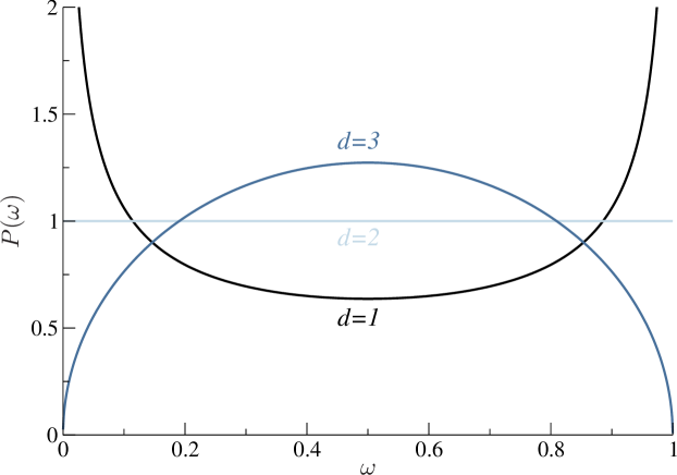
Figure 1: (Color online) The distribution $P(\omega)$ in Eq. (3.8) for $d=1,2$ and $3$.

4 The moment-generating function of the estimators.

Note that the Laplace transforms of quadratic functionals of Brownian motion (and other Gaussian processes), as the one in Eq. (3.1), have attracted a great deal of interest over the last decades following the pioneering work by Cameron and Martin [35]. Numerous results have been obtained both in the general setting of abstract Gaussian spaces and in various specific models generalising the original approach for Brownian motion due to Cameron and Martin (see, e.g., Refs.[36, 37, 38, 39] for contributions and references therein). An alternative approach is based on the path integrals formulation for quantum mechanics, which represents a powerful tool to analyse these problems using methods more familiar to physicists [40, 41]: here, the problem appears as the computation of the partition function of a quantum-harmonic oscillator with time dependent frequency. Various quadratic functionals of Brownian motion have been studied in details by physicists [42] with a variety of methods. They arise in a plethora of physical contexts, from polymers in elongational flows [43] to Casimir/van der Waals interactions and general fluctuation induced interactions [44, 45, 46, 47, 48] where, in the language of the harmonic oscillator, both the frequency and mass depend on time. Quadratic functionals of Brownian motion also arise in the theory of electrolytes when one computes the one-loop or fluctuation corrections to the mean field Poisson-Boltzmann theory [49, 50, 51, 52]. Finally we mention that functionals of Brownian motion also turn out to have applications in computer science [53].

In order to calculate $G(\sigma)$ in Eq. (3.4) we resort to the path integrals formulation. Following Refs.[29, 30], we introduce an auxiliary functional

$$\Psi(x,t)=\mathbb{E}^{x}_{t}\left\{\exp\left(-\frac{\sigma A_{\alpha}}{T}\int^{T}_{t}\,\omega(\tau)\,B_{\tau}^{2}\,d\tau\right)\right\}$$ (4.1)

where the expectation is for a Brownian motion starting at $x$ at time $t$. In terms of $\Psi(x,t)$ the moment-generating function is determined by noting that $G(\sigma)=\Psi(0,0)$.

Further on, we derive a Feynman-Kac type formula for $\Psi(x,t)$ considering how the functional in Eq. (4.1) evolves in the time interval $(t,t+dt)$. During this interval the Brownian motion moves from $x$ to $x+dB_{t}$, where $dB_{t}$ is an infinitesimal Brownian increment such that $\mathbb{E}_{dB}\{dB_{t}\}=0$ and $\mathbb{E}_{dB}\{dB^{2}_{t}\}=2Ddt$, where $\mathbb{E}_{dB}$ denotes now averaging with respect to the increment $dB_{t}$. For such an evolution we have, to linear order in $dt$

$$\Psi(x,t)=\mathbb{E}_{dB}\Big{\{}\left(1-\frac{\sigma A_{\alpha}\omega(t)}{T}x^{2}dt\right)\,\mathbb{E}^{x+dB_{t}}_{t+dt}\left\{\exp\left(-\frac{\sigma A_{\alpha}}{T}\int^{T}_{t+dt}\omega(\tau)\,B_{\tau}^{2}\,d\tau\right)\right\}\Big{\}}$$

$$=\mathbb{E}_{dB}\left\{\Psi(x+dB_{t},t+dt)\left(1-\frac{\sigma A_{\alpha}\omega(t)}{T}x^{2}dt\right)\right\}\,.$$ (4.2)

Expanding the right-hand-side of the latter equation to second order in $dB_{t}$ and to linear order in $dt$, we eventually find, after averaging, that $\Psi(x,t)$ obeys the equation

$$\frac{\partial\Psi(x,t)}{\partial t}=-D\frac{\partial^{2}\Psi(x,t)}{\partial x^{2}}+\frac{\sigma A_{\alpha}\omega(t)}{T}x^{2}\Psi(x,t)\,,$$ (4.3)

which looks like a Schrödinger equation with a harmonic time-dependent potential. Eq. (4.3) is to be solved subject to boundary condition $\Psi(x,T)=1$ for any $x$.

We seek the solution of Eq. (4.3) for arbitrary $\omega(t)$ in the form

$$\Psi(x,t)=f(t)\exp\left(-\frac{1}{2}g(t)x^{2}\right)\,,$$ (4.4)

where

$$\dot{f}=Dfg\,\,,f(t=T)=1\,,$$ (4.5)

and

$$\dot{g}=2Dg^{2}-\frac{\sigma\omega(t)}{dD\int^{T}_{0}\tau\omega(\tau)d\tau}\ ,\quad g(t=T)=0\,.$$ (4.6)

Next, we get rid of the nonlinearity in Eq.(4.6) introducing a new function $h$ obeying

$$g=-\frac{1}{2D}\frac{\dot{h}}{h}\,.$$ (4.7)

The function $h(t)$ is solution of the linear second-order differential equation

$$\ddot{h}-\frac{2\sigma\omega(t)}{d\int^{T}_{0}\tau\omega(\tau)d\tau}h=0\,,$$ (4.8)

which has to be solved subject to the boundary conditions

$$h(t=T)=1\,,\,\,\,\dot{h}(t=T)=0\,.$$ (4.9)

Once $h(t)$ is found, $f(t)$ is determined by $f(t)=1/\sqrt{h(t)}$ and $G(\sigma)$ by $G(\sigma)=f(0)=1/\sqrt{h(t=0)}$.

4.1 The moment-generating function for $\alpha\neq 2$.

We focus now on the particular case of the weight function $\omega(t)$ defined by Eq. (1.4) with $\alpha\neq 2$. In this case Eq. (4.8) reads

$$\ddot{h}-\frac{a\sigma}{\left(t_{0}+t\right)^{\alpha}}h=0\,,$$ (4.10)

with

$$a=\frac{2}{d\int^{T}_{0}\tau(t_{0}+\tau)^{-\alpha}d\tau}>0\,.$$ (4.11)

Solution of Eq.(4.10) has the form

$$h(t)=\sqrt{t_{0}+t}\left[C_{1}I_{\nu}\left(2\nu\sqrt{a(t_{0}+t)^{2-\alpha}\sigma}\right)+C_{2}K_{\nu}\left(2\nu\sqrt{a(t_{0}+t)^{2-\alpha}\sigma}\right)\right]\,,$$ (4.12)

where $I_{\mu}(\cdot)$ and $K_{\mu}(\cdot)$ are the modified Bessel functions [54], the exponent $\nu$ is given by

$$\nu=\frac{1}{2-\alpha}\,,$$ (4.13)

while the constants $C_{1}$ and $C_{2}$ are chosen to fulfil the boundary conditions in Eqs.(4.9), so that

$$C_{1}=2\nu\sqrt{a(t_{0}+T)^{1-\alpha}\sigma}K_{\nu-1}\left(2\nu\sqrt{a(t_{0}+T)^{2-\alpha}\sigma}\right)\,,$$ (4.14)

and

$$C_{2}=2\nu\sqrt{a(t_{0}+T)^{1-\alpha}\sigma}I_{\nu-1}\left(2\nu\sqrt{a(t_{0}+T)^{2-\alpha}\sigma}\right)\,.$$ (4.15)

Consequently, we find that $h(t=0)$ obeys

$$h(t=0) = \left(\frac{\epsilon}{1+\epsilon}\right)^{(\alpha-1)/2}\frac{\pi\nu z\sqrt{\sigma}}{2\sin\left(\pi\nu\right)}\times$$ (4.16)

$$\times \Big{[}I_{-\nu}\left(\nu z\sqrt{\sigma}\right)I_{\nu-1}\left(\left(\frac{1+\epsilon}{\epsilon}\right)^{1-\alpha/2}\nu z\sqrt{\sigma}\right)-$$

$$- I_{\nu}\left(\nu z\sqrt{\sigma}\right)I_{1-\nu}\left(\left(\frac{1+\epsilon}{\epsilon}\right)^{1-\alpha/2}\nu z\sqrt{\sigma}\right)\Big{]}\,,$$

where $\epsilon=t_{0}/T$, and

$$z=\sqrt{\frac{8(1-\alpha)(2-\alpha)\epsilon^{2-\alpha}}{d\left(\epsilon^{2-\alpha}-(\alpha+\epsilon-1)(1+\epsilon)^{1-\alpha}\right)}}\,.$$ (4.17)

Turning finally to the limit $\epsilon\to 0$, we find that the leading small-$\epsilon$ behaviour of the moment-generating function is given by

$$\Phi(\sigma)=\left[\Gamma\left(\nu\right)\left(\frac{\sigma}{\chi_{1}}\right)^{\frac{1-\nu}{2}}{\rm I}_{\nu-1}\left(2\sqrt{\frac{\sigma}{\chi_{1}}}\right)\right]^{-d/2}\,,$$ (4.18)

for $\alpha<2$, while for $\alpha>2$ it obeys

$$\Phi(\sigma)=\left[\Gamma\left(1-\nu\right)\left(\frac{\sigma}{\chi_{2}}\right)^{\frac{\nu}{2}}{\rm I}_{-\nu}\left(2\sqrt{\frac{\sigma}{\chi_{2}}}\right)\right]^{-d/2}\,,$$ (4.19)

where

$$\chi_{1}=\frac{d(2-\alpha)}{2}\,\,\,\,{\rm and}\,\,\,\chi_{2}=\frac{d(\alpha-2)}{2(\alpha-1)}\,.$$ (4.20)

4.2 The moment-generating function for $\alpha=2$.

We focus next on the particular case $\alpha=2$ and consider for convenience a slightly more general form of the weight function $\omega(t)$ by introducing an additional parameter $\xi$. We stipulate that $\omega(t)$ is the piece-wise continuous function

$$\omega(t)=\cases{2\xi/t_{0}^{2},&for $0\leq t\leq t_{0}$,\\ 1/t^{2},&for $t_{0}\leq t\leq T$.}$$ (4.21)

We seek now the corresponding moment-generating function $\Phi(\sigma)$ and optimise it in what follows considering $\xi$ as an optimisation parameter.

The differential Eq. (4.8) has to be solved now for two intervals $t\in[0,t_{0}]$ and $t\in[t_{0},T]$ in which the ”potential” has two different forms. For the first interval, i.e., when $t\in[0,t_{0}]$, the general solution of Eq. (4.8) obeys

$$h(t)=c_{1}\,\exp\left(-\sqrt{2a\xi\sigma}\,\frac{t}{t_{0}}\right)+c_{2}\,\exp\left(\sqrt{2a\xi\sigma}\,\frac{t}{t_{0}}\right)\,,$$ (4.22)

where $c_{1}$ and $c_{2}$ are coefficients to be determined. The parameter $a$ given by Eq. (4.11) now reads

$$a=\frac{2}{d(\xi+\ln\left(1/\epsilon\right))}\,.$$ (4.23)

For the second interval, i.e., when $t$ belongs to $[t_{0},T]$, we have

$$h(t)=c_{3}\,t^{(1+\delta)/2}+c_{4}\,t^{(1-\delta)/2}\,,$$ (4.24)

where

$$\delta=\sqrt{1+4a\sigma}\,,$$ (4.25)

while the coefficients $c_{3}$ and $c_{4}$ are to be found from the boundary conditions in Eqs. (4.9). This yields

$$c_{3}=\frac{\delta-1}{2\delta}\,T^{-(1+\delta)/2}\,,$$ (4.26)

and

$$c_{4}=\frac{\delta+1}{2\delta}\,T^{(\delta-1)/2}\,.$$ (4.27)

Further on, we require the continuity of $h(t)$ and its first derivative at $t=t_{0}$. We find then that

$$c_{1}=\frac{(\delta+1)\exp\left(\sqrt{2a\xi\sigma}\right)}{4\delta\epsilon^{(\delta-1)/2}}\,\left(1+\frac{\delta-1}{\delta+1}\epsilon^{\delta}-\frac{\delta-1}{2\sqrt{2a\xi\sigma}}\left(1+\epsilon^{\delta}\right)\right)$$ (4.28)

and

$$c_{2}=\frac{(\delta+1)\exp\left(-\sqrt{2a\xi\sigma}\right)}{4\delta\epsilon^{(\delta-1)/2}}\,\left(1+\frac{\delta-1}{\delta+1}\epsilon^{\delta}+\frac{\delta-1}{2\sqrt{2a\xi\sigma}}\left(1+\epsilon^{\delta}\right)\right)\,.$$ (4.29)

Consequently, we find that in this case the moment-generating function is given for arbitrary $\epsilon$ explicitly by

$$\Phi(\sigma)=\left(c_{1}+c_{2}\right)^{-d/2} = \Big{[}\frac{(\delta+1)}{2\delta\epsilon^{(\delta-1)/2}}\Big{(}\Big{(}1+\frac{\delta-1}{\delta+1}\epsilon^{\delta}\Big{)}\,\cosh\left(\sqrt{2a\xi\sigma}\right)+$$ (4.30)

$$+ \frac{\delta-1}{2\sqrt{2a\xi\sigma}}\left(1+\epsilon^{\delta}\right)\,\sinh\left(\sqrt{2a\xi\sigma}\right)\Big{)}\Big{]}^{-d/2}\,.$$

Now, we are equipped with all necessary results to determine the variance of the distribution $P(u_{\alpha})$ as well as the distribution itself.

5 The variance of the distribution $P(u_{\alpha})$.

In this section we analyse the behaviour of the variance ${\rm Var}(u_{\alpha})$ of the estimator in Eq. (1.3). First, we calculate exactly the limiting small-$\epsilon$ form of ${\rm Var}(u_{\alpha})$ for arbitrary $\alpha\neq 2$. Further on, we focus on the case $\alpha=2$ and determine ${\rm Var}(u_{\alpha=2})$ for arbitrary $\epsilon$ and $\xi$, Eq. (4.21). We show next that the variance has a minimum for a certain amplitude $\xi=\xi_{\rm opt}$ and present a corresponding expression for the optimised variance. Finally, we consider the case when the continuous-space and -time trajectory is recorded at arbitrary discrete time moments $t_{j}$ and calculate exactly the weight function $\omega(t)$ which provides the minimal possible variance.

5.1 The variance for $\alpha\neq 2$ and $\epsilon=0$.

The variance ${\rm Var}(u_{\alpha})$ is obtained by differentiating Eqs. (4.18) or (4.19) twice with respect to $\sigma$ and setting $\sigma$ equal to zero. For arbitrary $\alpha\neq 2$ the variance is then given explicitly by

$${\rm Var}(u_{\alpha})=\frac{2}{d}\cases{\frac{2-\alpha}{3-\alpha},&for $\alpha<2$,\\ \frac{\alpha-2}{2\alpha-3},&for $\alpha>2$.}$$ (5.1)

The result in the latter equation is depicted in Fig. 2 and shows that, strikingly, the variance can be made arbitrarily small in the leading order in $\epsilon$ by taking $\alpha$ gradually closer to $2$, either from above or from below. The slopes at $\alpha=2^{+}$ and $\alpha=2^{-}$ appear to be the same, so that the accuracy of the estimator will be the same for approaching $\alpha=2$ from above or from below. Equation (5.1), although formally invalid for $\alpha=2$, also suggests that the estimator in Eq. (1.3) with $\alpha=2$ has vanishing variance and thus possesses an ergodic property.

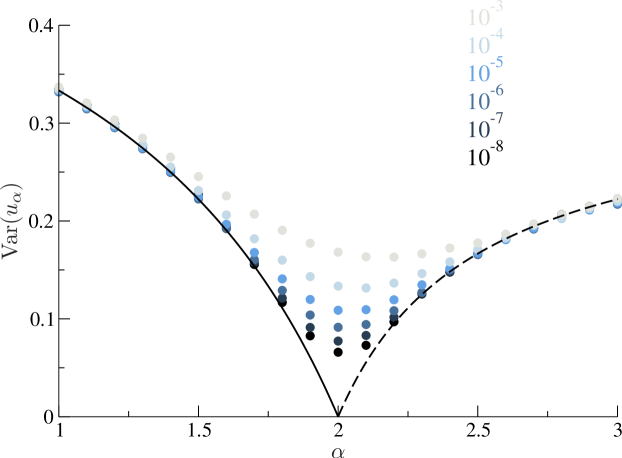
Figure 2: (Color online) The variance of the distribution $P(u_{\alpha})$ in $d=3$ for different values of $\alpha$. Solid line - Eq. (5.1) with $\alpha<2$ and the dashed line - Eq. (5.1) with $\alpha>2$. The symbols correspond to the values obtained from numerical simulations of 3D random walks for different $\epsilon$, as indicated by the labels.

A word of caution is now in order. As a matter of fact, we deduce from Eq. (4.16) that finite-$\epsilon$ corrections to the result in Eq. (5.1) are of order of $\mathcal{O}(\epsilon^{2-\alpha})$ for $1<\alpha<2$, which means that this asymptotical behaviour can be only attained when $\epsilon\ll\exp\left(-1/(2-\alpha)\right)$. In other words, the variance can be made arbitrarily small by choosing $\alpha$ closer to $2$, but only at expense of either decreasing the experimental resolution time $t_{0}$ or increasing the observation time $T$, which is clearly seen from the numerical data shown in Fig. 2.

5.2 The variance for $\alpha=2$ and arbitrary $\epsilon$.

Differentiating Eq. (4.30) with respect to $\sigma$ twice, we find that for arbitrary $\epsilon$ the variance of the distribution $P(u_{2})$ is given explicitly by

$${\rm Var}(u_{2})=\frac{4}{3d}\,\frac{3\ln(1/\epsilon)-3(1-\epsilon)+2(1-\epsilon)\xi+\xi^{2}}{\left(\xi+\ln(1/\epsilon)\right)^{2}}\,.$$ (5.2)

Notice now that ${\rm Var}(u_{2})$ in Eq. (5.2) is a non-monotonic function of $\xi$ which attains its minimal value when

$$\xi=\xi_{{\rm opt}}=\frac{(2+\epsilon)\ln(1/\epsilon)-3(1-\epsilon)}{\ln(1/\epsilon)+\epsilon-1}\,.$$ (5.3)

This is a somewhat surprising result which states that the optimal choice of the amplitude $\xi$ in Eq. (4.21), which defines the weight function $\omega(t)$, actually depends on both the time lag $t_{0}$ and on the observation time $T$. In other words, in order to make a proper choice of the amplitude $\xi$, one has to know in advance the time through which the trajectory is observed. Similar dependence of the optimal parameters on the observation time has been recently reported in Refs.[56, 57], which optimised the number of distinct sites visited by intermittent random walks. Note that $\xi_{\rm opt}\to 2$ as $\epsilon\to 0$, but for any finite $\epsilon$ it is greater than $2$.

Plugging the expression in Eq. (5.3) into the Eq. (5.2) we obtain the corresponding optimised variance

$${\rm Var}_{\rm opt}(u_{2})=\frac{4}{3d}\,\frac{3\ln(1/\epsilon)-4+5\epsilon-\epsilon^{2}}{\ln(1/\epsilon)\left(\ln(1/\epsilon)+1+2\epsilon\right)-3(1-\epsilon)}\,.$$ (5.4)

From Eq. (5.4) we find that in 3D ${\rm Var}_{\rm opt}(u_{2})\approx 0.144$ for $\epsilon=10^{-3}$, ${\rm Var}_{\rm opt}(u_{2})\approx 0.096$ for $\epsilon=10^{-5}$ and ${\rm Var}_{\rm opt}(u_{2})\approx 0.082$ for $\epsilon=10^{-6}$. When $\epsilon\to 0$, ${\rm Var}_{\rm opt}(u_{2})$ vanishes in a logarithmic way with $\epsilon$ at leading order:

$${\rm Var}_{\rm opt}(u_{2})\sim\frac{4}{d}\frac{1}{\ln(1/\epsilon)}\,.$$ (5.5)

Therefore, the variance can be made arbitrarily small but at expense of a progressively higher resolution or a larger observation time. Note that this is the only case ($\alpha=2$) in which the estimator defined by Eq. (1.3) is ergodic.

5.3 Optimisation of the variance for continuous-time and -space trajectories recorded at discrete time moments.

Finally we consider the estimation of the diffusion constant $D_{f}$ when one has a set of $N$ temporal points $t_{j}$ such that $0<t_{0}<t_{1}<\cdots<t_{N-1}=T$ and a value $B_{t_{j}}^{2}$, (which is one of the components of $d$-dimensional Brownian motion), for each of these points. We consider the least-squares estimator

$$u_{\rm dis}={1\over 2}\sum_{j=0}^{N-1}\omega_{j}\,B^{2}_{t_{j}}\,,$$ (5.6)

where the normalisation is now adsorbed into the weight function $\omega_{j}$, so that

$${1\over 2}\sum_{j=0}^{N-1}\omega_{j}\,\mathbb{E}\{B^{2}_{t_{j}}\}=1$$ (5.7)

As in the previous subsection, we seek an optimal weight function $\omega_{j}$ which minimises the variance of the least-squares estimator in Eq. (5.6). Remarkably, this problem can be solved exactly for any arbitrary set $\{t_{j}\}$.

The variance of this estimator can be straightforwardly calculated explicitly, for arbitrary $\omega_{j}$, to give

$${\rm Var}(u_{\rm dis})=2\sum_{j,k}\omega_{j}\,\omega_{k}\,(t_{j}\wedge t_{k})^{2}\,,$$ (5.8)

where $(t_{j}\wedge t_{k})$ equals the smallest of two numbers $t_{j}$ and $t_{k}$.

In order to determine the choice of the $\omega_{j}$ which minimises the variance of the estimator, we minimise the functional

$$F={1\over 2}\sum_{j,k}\omega_{j}\,(t_{j}\wedge t_{k})^{2}\,\omega_{k}-\lambda\left(\sum_{j=0}^{N-1}\omega_{j}t_{j}-1\right)\,,$$ (5.9)

where $\lambda$ is a Lagrange multiplier enforcing Eq. (5.7). Minimising with respect to each $\omega_{j}$ gives the system of linear equations

$$\sum_{j}(t_{j}\wedge t_{k})^{2}\omega_{j}=\lambda\,t_{k}.$$ (5.10)

To solve this system of equations exactly, we define

$$\Omega_{k}=\sum_{j\geq k}\omega_{j}\,,$$ (5.11)

or, equivalently,

$$\omega_{j}=\Omega_{j}-\Omega_{j+1}\,,$$ (5.12)

for $0\leq j\leq N-2$. Also clearly we have that $\Omega_{N-1}=\omega_{N-1}$ which is compatible with defining $\Omega_{N}=0$. Therefore Eq. (5.10) can be written as

$$\sum_{j<k}(\Omega_{j}-\Omega_{j+1})t_{j}^{2}+t_{k}^{2}\Omega_{k}=\lambda t_{k}.$$ (5.13)

Now subtracting Eq. (5.13) for $k$ from the same equation for $k+1$ gives the solution

$$\Omega_{k+1}={\lambda\over t_{k+1}+t_{k}},$$ (5.14)

valid for $0\leq k\leq N-2$, which implies that

$$\Omega_{k}={\lambda\over t_{k}+t_{k-1}}$$ (5.15)

which is valid for $1\leq k\leq N-1$. In addition, if we set $k=0$ in Eq. (5.13) we find that

$$\Omega_{0}={\lambda\over t_{0}},$$ (5.16)

which is compatible with Eq. (5.15) upon defining an additional point $t_{-1}=0$. We thus find that for $1\leq j\leq N-2$,

$$\omega_{j}=\Omega_{j}-\Omega_{j+1}={\lambda\over(t_{j}+t_{j-1})}-{\lambda\over(t_{j}+t_{j+1})}\,,$$ (5.17)

while

$$\omega_{0}={\lambda t_{1}\over t_{0}(t_{0}+t_{1})}\,,$$ (5.18)

and

$$\omega_{N-1}=\Omega_{N-1}={\lambda\over t_{N-1}+t_{N-2}}\,.$$ (5.19)

The normalisation constraint, Eq. (5.7), then yields $\lambda$ as

$$\lambda=\left({t_{1}\over t_{0}+t_{1}}+{t_{N-1}\over t_{N-1}+t_{N-2}}+\sum_{j=1}^{N-2}{t_{j}(t_{j+1}-t_{j-1})\over(t_{j+1}+t_{j})(t_{j}+t_{j-1})}\right)^{-1}.$$ (5.20)

Finally the minimal variance can be computed by multiplying Eq.(5.10) by $\omega_{k}$ and summing over $k$ which gives

$$\sum_{j,k}\omega_{j}\,(t_{j}\wedge t_{k})^{2}\omega_{k}=\lambda\,\sum_{j=0}^{N-1}\omega_{j}\,t_{j}=\lambda\,,$$ (5.21)

and hence,

$${\rm Var}(u_{\rm dis})=2\sum_{j,k}\omega_{j}\,\omega_{k}(t_{j}\wedge t_{k})^{2}=2\,\lambda\,,$$ (5.22)

where we have again used the normalisation condition Eq. (5.7). Equations (5.17) to (5.20) define the exact solution of the problem of the optimal estimator for Brownian trajectories recorded at discrete time moments.

In order to compare the results with the continuum case we take the first point $t_{0}$ to be fixed and write $t_{j}=t_{0}+\Delta(j-1)$ for $j>0$, where $\Delta$ is a constant time step, $\Delta=T/(N-1)$. This gives the following expression for the Lagrange multiplier, which defines the variance of the distribution,

$$\lambda=\left({t_{0}\over 2t_{0}+\Delta}+{T\over 2T-\Delta}+2\Delta\,\sum_{j=1}^{N-2}{t_{0}+(j-1)\Delta\over(2t_{0}+(2j-1)\Delta)(2t_{0}+(2j+1)\Delta)}\right)^{-1}\,.$$ (5.23)

Turning to the limit $\Delta\to 0$ and $N\to\infty$, but keeping the ratio $T=N/\Delta$ fixed, the sum in the latter equation becomes a Riemann integral and we find

$$\lambda^{-1}=1+{1\over 2}\int_{t_{0}}^{T}{dt\over t}=1+{1\over 2}\ln({T\over t_{0}})\,,$$ (5.24)

so that in the leading in $\epsilon$ order, for $d$-dimensional systems,

$${\rm Var}(u_{\rm dis})={4\over d\left(2+\ln({1/\epsilon})\right)}\,.$$ (5.25)

Note that for $\ln(1/\epsilon)\gg 2$, the latter equation exhibits exactly the same asymptotic behaviour in the limit $\epsilon\to 0$, as the result of the previous Section 5.2, Eq. (5.5).

6 Tails of the distribution $P(u_{\alpha})$ in $d$ dimensions

Exact expressions for the moment-generating function allow us to deduce the asymptotic behaviour of the distribution $P(u_{\alpha})$ for $u_{\alpha}\ll 1$ and $u_{\alpha}\gg 1$.

6.1 Asymptotic behaviour of $P(u_{\alpha})$ for $\alpha\neq 2$ and $\epsilon=0$.

Large- and small-$u_{\alpha}$ asymptotics of $P(u_{\alpha})$ can be deduced directly from Eqs. (4.18) and (4.19). Let us first focus on the small-$u_{\alpha}$ behaviour, which stems from the large-$\sigma$ asymptotical behaviour of the moment-generating function. For $\alpha<2$ the latter obeys

$$\Phi(\sigma)\sim\sigma^{d(1+2/(2-\alpha))/8}\,\exp\left(-\sqrt{\frac{2d\sigma}{2-\alpha}}\right)\,.$$ (6.1)

Inverting Eq. (6.1) we find that for $u_{\alpha}\to 0$ and $\alpha<2$ the distribution $P(u_{\alpha})$ shows a singular behaviour:

$$P(u_{\alpha})\sim\exp\left(-\frac{d^{2}}{4\chi_{1}}\cdot\frac{1}{u_{\alpha}}\right)\frac{1}{u_{\alpha}^{\zeta}}\,,$$ (6.2)

where the exponent $\zeta$ is given by

$$\zeta=\frac{3}{2}+\frac{d}{4}\frac{\alpha}{|2-\alpha|}\,,$$ (6.3)

and the parameter $\chi_{1}$ is defined in Eq. (4.20). The analogous left tail for $\alpha>2$ case can be obtained from Eq. (6.2) by simply making the replacement $\chi_{1}\to\chi_{2}$.

Note that Eq. (6.2) describes a bell-shaped function whose maximum gives an approximation to the most probable value of the estimator $u$

$$u^{*}=\frac{2d}{\alpha d+6|2-\alpha|}$$ (6.4)

Note that for any fixed $d$ and $\alpha\to 2$, the most probable $u^{*}\to 1$, i.e. to the ensemble average value of the estimator in Eq. (1.3). Therefore, the least-squares estimators outperform the naive end-to-end estimator of the diffusion coefficient, whose distribution is given in Eq. (1.2) and has a bell-shaped form only for $d\geq 3$.

Next, we turn to the large-$u_{\alpha}$ asymptotical behaviour of the distribution function. To do this, it is convenient to rewrite the result in Eq. (4.18) as

$$\Phi(\sigma)=\prod_{m=1}^{\infty}\left(1+8\sigma/(2-\alpha)d\gamma^{2}_{\nu-1,m}\right)^{-d/2}\,,$$ (6.5)

where $\gamma_{\mu,m}$ is the $m$-th zero of the Bessel function $J_{\mu}(z)$, organised in an ascending order [54]. The large-$u_{\alpha}$ behaviour of the distribution function stems from the behaviour of the moment-generating function in the vicinity of the singular point on the negative $\sigma$-axis which is closest to $\sigma=0$ (all singularities are all located on the negative $\sigma$-axis). This yields, for $\alpha<2$, an exponential decay of the form

$$P(u_{\alpha})\sim u_{\alpha}^{d/2-1}\exp\left(-\frac{\chi_{1}\gamma_{\nu-1,1}^{2}}{4}\cdot u_{\alpha}\right)\,.$$ (6.6)

In a similar fashion, we get that for $\alpha>2$ the moment-generating function can be represented as

$$\Phi(\sigma)=\prod_{m=1}^{\infty}\left(1+8(\alpha-1)\sigma/(\alpha-2)d\gamma^{2}_{-\nu,m}\right)^{-d/2}\,,$$ (6.7)

so that in this case the right tail of $P(u_{\alpha})$ follows

$$P(u_{\alpha})\sim u_{\alpha}^{d/2-1}\exp\left(-\frac{\chi_{2}\gamma_{-\nu,1}^{2}}{4}\cdot u_{\alpha}\right)\,.$$ (6.8)

To summarise the results of this subsection, we note the following:

• when $\alpha\to 2$, either from above or from below, the small-$u_{\alpha}$ behaviour of $P(u_{\alpha})$ becomes progressively more singular and small values of $u_{\alpha}$ become very unlikely since both $\chi_{1}$ and $\chi_{2}$ tend to zero and the exponent $\zeta$ diverges.

• when $\alpha\to 2$, either from above or from below, the inverse relaxation ”lengths” (i.e., the terms $(\alpha-2)\gamma_{-\nu,1}^{2}$ and $(2-\alpha)\gamma_{\nu-1,1}^{2}$ in the exponentials in Eqs. (6.6) and (6.8)) diverge, suppressing large values of $u_{\alpha}$ in the distribution.

Since $P(u_{\alpha})$ is normalised for arbitrary $\alpha$, so that the area below the curve is fixed, this implies that $P(u_{\alpha})$ tends to the delta-function as $\alpha\to 2$.

6.2 Asymptotic behaviour of $P(u_{\alpha})$ for $\alpha=2$ and small $\epsilon$.

We focus first on the left tails of the distribution for $\alpha=2$ and fixed small $\epsilon$. From Eq. (4.30) we find that in the limit $\sigma\to\infty$ (so that $\delta$ in Eq. (4.25) is $\delta\gg 1$), fixed sufficiently small $\epsilon$, the moment-generating function obeys

$$\Phi(\sigma)\sim\exp\left(-\sqrt{\frac{d\,\ln(1/\epsilon)}{2}\cdot\sigma}\right)\,,$$ (6.9)

from which equation we readily obtain the following singular form:

$$P(u_{2})\sim\exp\left(-\frac{d\ln(1/\epsilon)}{8}\cdot\frac{1}{u_{2}}\right)\frac{1}{u_{2}^{3/2}}\,,$$ (6.10)

which holds for $u_{2}\ll 1$. Within the opposite limit, i.e., for $u_{2}\gg 1$, the leading behaviour of the distribution $P(u_{2})$ is dominated by the closest to the origin root of the denominator in Eq. (4.30). Some algebra gives that for $\epsilon\to 0$ the distribution function $P(u_{2})$ has the following simple form

$$P(u_{2})\sim u_{2}^{d/2-1}\exp\left(-\frac{d\,x_{0}^{2}\left(\xi_{\rm opt}+\ln(1/\epsilon)\right)}{4\,\xi_{\rm opt}}\cdot u_{2}\right)\,,$$ (6.11)

where $\xi_{\rm opt}$ is the optimised amplitude in Eq. (5.3) and $x_{0}$, in the limit $\epsilon\to 0$, is the root of the equation

$$\left(1-\frac{2x_{0}^{2}}{\xi_{\rm opt}}\right)^{1/2}\,\frac{x_{0}\cos\left(x_{0}\right)}{\sin\left(x_{0}\right)}=\frac{1}{2+\ln(1/\epsilon)}$$ (6.12)

The asymptotic behaviour of $x_{0}$ can be readily obtained:

$$x_{0}=\sqrt{\frac{\xi_{\rm opt}}{2}}\left(1-\frac{1}{\xi_{\rm opt}\,\cot^{2}\left(\sqrt{\xi_{\rm opt}/2}\right)\,\left(2+\ln(1/\epsilon)\right)^{2}}+\mathcal{O}\left(\frac{1}{\ln^{4}(1/\epsilon)}\right)\right)\,.$$ (6.13)

Therefore, the characteristic decay lengths of the distribution $P(u_{2})$ from both sides from the maximum vanish as $1/\ln(1/\epsilon)$ when $\epsilon\to 0$.

7 The distribution $P(u_{\alpha})$ in $d$ dimensions

We turn now to the inversion of the Laplace transform in Eq. (3.1) in order to visualise the full distribution $P(u_{\alpha})$ and to get an idea of the location of most probable values of the estimators in Eq. (1.3).

7.1 Inversion of the Laplace transform for $\alpha\neq 2$

As we have already remarked, all poles of the moment-generating function $\Phi(\sigma)$ lie on the complex plane on the negative real $\sigma$-axis, as can be readily seen from the representations in Eqs. (6.5) and (6.7). Setting then $\gamma=0$ in Eq. (3.5), we find

$$P(u_{\alpha})=\frac{1}{\pi}\int^{\infty}_{0}\frac{dz\,\cos\left(zu_{\alpha}-d\,\phi_{\alpha}(z)/2\right)}{\rho_{\alpha}^{d/4}(z)},$$ (7.1)

where, for $\alpha<2$,

$$\rho_{\alpha}(z)=\Gamma^{2}\left(\nu\right)\left(\frac{\chi_{1}}{z}\right)^{\nu-1}\,\left({\rm ber}_{\nu-1}^{2}\left(2\,\sqrt{\frac{z}{\chi_{1}}}\right)+{\rm bei}_{\nu-1}^{2}\left(2\,\sqrt{\frac{z}{\chi_{1}}}\right)\right)\,,$$ (7.2)

and the phase $\phi$ is given by

$$\phi_{\alpha}(z)={\rm arctg}\left({\rm ber}_{\nu-1}\left(2\,\sqrt{\frac{z}{\chi_{1}}}\right)/{\rm ber}_{\nu-1}\left(2\,\sqrt{\frac{z}{\chi_{1}}}\right)\right)\,,$$ (7.3)

while for $\alpha>2$ we have

$$\rho_{\alpha}(z)=\Gamma^{2}\left(1-\nu\right)\left(\frac{\chi_{2}}{z}\right)^{-\nu}\,\left({\rm ber}_{-\nu}^{2}\left(2\,\sqrt{\frac{z}{\chi_{2}}}\right)+{\rm bei}_{-\nu}^{2}\left(2\,\sqrt{\frac{z}{\chi_{2}}}\right)\right)\,,$$ (7.4)

and

$$\phi_{\alpha}(z)={\rm arctg}\left({\rm ber}_{-\nu}\left(2\,\sqrt{\frac{z}{\chi_{2}}}\right)/{\rm ber}_{-\nu}\left(2\sqrt{\frac{z}{\chi_{2}}}\right)\right)\,,$$ (7.5)

where ${\rm ber}_{\mu}(x)$ and ${\rm bei}_{\mu}(x)$ are the Kelvin functions [54]. Equation (7.1) defines the probability distributions $P(u_{\alpha})$ in the leading in $\epsilon$ order for arbitrary $\alpha\neq 2$ and arbitrary spatial dimension $d$.

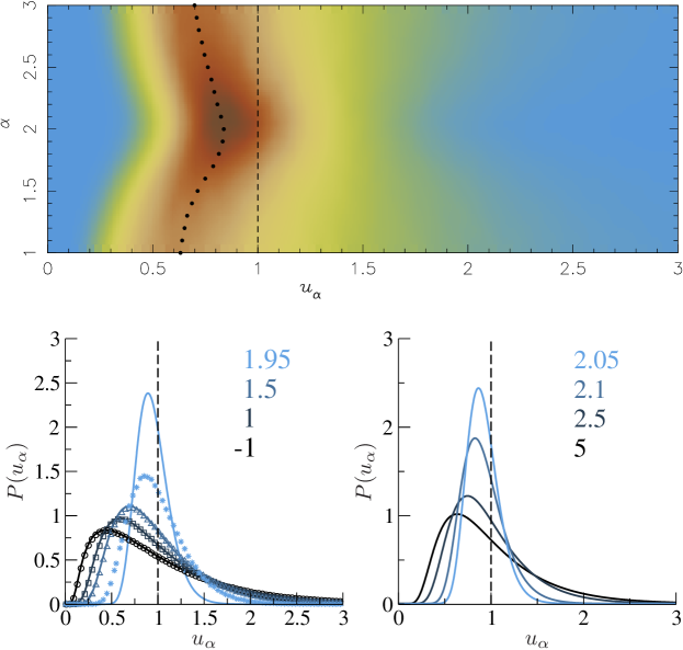
Figure 3: (Color online) The distribution $P(u_{\alpha})$ in 3D systems. Upper panel: Colour density map of $P(u_{\alpha})$ as a function of $\alpha$, obtained from numerical simulations of 3D random walks, with $\epsilon=10^{-5}$. The solid knots indicate, for different values of $\alpha$, the position of the most probable value of the estimator $u_{\alpha}$. Lower panel: The distribution $P(u_{\alpha})$ for different $\alpha\neq 2$ and with $\epsilon=0$, obtained by numerical inversion of Eq. (7.1) for $\alpha<2$ (left lower panel) and of Eq. (7.1) for $\alpha>2$ (right lower panel). The symbols in the left panel correspond to numerical simulations for (from dark to light), $\alpha=-1$ (circles), $\alpha=1$ (squares), $\alpha=3/2$ (triangles), and $\alpha=1.95$ (stars), and $\epsilon=10^{-5}$, except for $\alpha=1.95$ for which we used $\epsilon=10^{-7}$.

In Fig. 3 we plot $P(u_{\alpha})$ from Eq. (7.1) for $\alpha\neq 2$ and $\epsilon=0$ for three-dimensional systems together with the results of numerical simulations. One notices that the theoretically predicted distribution $P(u_{\alpha})$ becomes more narrow and its maximal value grows when $\alpha$ moves towards $\alpha=2$, either from above or from below. When $\alpha$ approaches $2$ from below, the most probable value moves toward the ensemble average value ($=1$) of the estimator and then starts to move back when $\alpha$ overpasses $2$ and grows further. Similarly to the behaviour of the variance, we observe a very good agreement between our theoretical predictions and numerical data for $\alpha$ not too close to $2$ for $\epsilon=10^{-5}$ (lower left panel of Fig.3). For $\alpha=1.95$ and $\epsilon$ as small as $10^{-7}$, we still see a discrepancy between the numerical data and the asymptotic form of $P(u_{\alpha})$ in Eq. (7.1). Note that the same slow convergence to zero variance was observed in Fig.2 as $\epsilon\to 0$.

Figure 4: (color online) The distribution $P(\omega_{\alpha})$ in Eq. (3.7) for different $\alpha<2$ in 3D systems. Symbols are the results of numerical simulations. The dashed curve is the corresponding result for the end-to-end estimate of the diffusion coefficient in Eq. (3.8).

In Fig.4 we present the results of numerical simulations for the distribution in Eq. (3.7) of the random variable $\omega$ defined in Eq. (3.6). One notices that as $\alpha\to 2$, the distribution becomes progressively narrower and the peak at $\omega=1/2$ becomes more pronounced, which means that it becomes progressively more likely that the diffusion coefficients, deduced from two different realisations of Brownian trajectories using the weighted least-squares estimators, will have the same value.

7.2 Two-dimensional systems: series representation of the distributions $P(u_{\alpha})$ and $P(\omega_{\alpha})$

We proceed further and focus now on the case $d=2$ when $\Phi(\sigma)$ in Eqs. (6.5) and (6.7) have only simple poles. In this case, we readily find via standard residue calculus

$$P(u_{\alpha})=\frac{2^{-\nu}}{\Gamma(\nu+1)}\,\sum_{m=1}^{\infty}\frac{\gamma^{\nu}_{\nu-1,m}}{J_{\nu}\left(\gamma_{\nu-1,m}\right)}\,\exp\left(-\frac{(2-\alpha)\gamma^{2}_{\nu-1,m}}{4}u_{\alpha}\right)\,,$$ (7.6)

for $\alpha<2$, while for $\alpha>2$ we get

$$P(u_{\alpha})=\frac{2^{\nu-1}}{\Gamma(2-\nu)}\,\sum_{m=1}^{\infty}\frac{\gamma^{1-\nu}_{-\nu,m}}{J_{1-\nu}\left(\gamma_{-\nu,m}\right)}\,\exp\left(-\frac{(\alpha-2)\gamma^{2}_{-\nu,m}}{(\alpha-1)4}u_{\alpha}\right)\,.$$ (7.7)

These expressions can be readily plotted using, e.g., Mathematica, and they show exactly the same qualitative behaviour (apart from a slightly larger variance), as our results obtained by the inversion of the Laplace transform for three-dimensional systems (see, Fig. 3).

We finally present explicit results for the distribution $P(\omega_{\alpha})$, Eq. (1.4), for two-dimensional systems. For $P(u_{\alpha})$ in Eq. (7.6) one has, using the definition in Eq. (3.7),

$$P(\omega_{\alpha}) = \left(\frac{2^{-\nu}}{\Gamma\left(\nu+1\right)\,(1-\omega_{\alpha})}\right)^{2}\,\sum_{n=1}^{\infty}\frac{\gamma^{\nu}_{\nu-1,n}}{J_{\nu}\left(\gamma_{\nu-1,n}\right)}\,\sum_{m=1}^{\infty}\frac{\gamma^{\nu}_{\nu-1,m}}{J_{\nu}\left(\gamma_{\nu-1,m}\right)}$$ (7.8)

$$\times \int_{0}^{\infty}u_{\alpha}\,du_{\alpha}\,\exp\left(-\frac{(2-\alpha)}{4}\,\left(\frac{\omega_{\alpha}}{1-\omega_{\alpha}}\,\gamma^{2}_{\nu-1,n}+\gamma^{2}_{\nu-1,m}\right)\,u_{\alpha}\right)$$

$$= \left(\frac{2^{2-\nu}}{(2-\alpha)\,\Gamma\left(\nu+1\right)}\right)^{2}\,\sum_{n=1}^{\infty}\frac{\gamma^{\nu}_{\nu-1,n}}{J_{\nu}\left(\gamma_{\nu-1,n}\right)}$$

$$\times \sum_{m=1}^{\infty}\frac{\gamma^{\nu}_{\nu-1,m}}{J_{\nu}\left(\gamma_{\nu-1,m}\right)}\,\frac{1}{\left(\omega_{\alpha}\gamma^{2}_{\nu-1,n}+(1-\omega_{\alpha})\gamma^{2}_{\nu-1,m}\right)^{2}}\,.$$

Further on, making use of the following equality

$$\frac{1}{\gamma^{2}_{\nu-1,m}}\,\frac{d}{d\omega_{\alpha}}\,\left(\gamma^{2}_{\nu-1,n}+\frac{(1-\omega_{\alpha})}{\omega_{\alpha}}\gamma^{2}_{\nu-1,m}\right)^{-1}=\frac{1}{\left(\omega_{\alpha}\gamma^{2}_{\nu-1,n}+(1-\omega_{\alpha})\gamma^{2}_{\nu-1,m}\right)^{2}}$$ (7.9)

and of the definition of the moment-generating function, Eq. (4.18),

$$\Phi(\sigma) = \int^{\infty}_{0}du_{\alpha}\,P(u_{\alpha})\,\exp\left(-\sigma\,u_{\alpha}\right)$$ (7.10)

$$= \left[\Gamma\left(\nu\right)\left(\frac{\sigma}{2-\alpha}\right)^{\frac{1-\nu}{2}}{\rm I}_{\nu-1}\left(2\sqrt{\frac{\sigma}{2-\alpha}}\right)\right]^{-1}$$

$$= \frac{2^{2-\nu}}{(2-\alpha)\,\Gamma(\nu+1)}\,\sum_{n=1}^{\infty}\frac{\gamma^{\nu}_{\nu-1,n}}{J_{\nu}\left(\gamma_{\nu-1,n}\right)}\,\left(\frac{4\sigma}{2-\alpha}+\gamma^{2}_{\nu-1,n}\right)^{-1}\,,$$

we can perform one of the summations in Eq. (7.8) and, finally, expressing the Bessel functions in terms of hypergeometric series, we find

$$P(\omega_{\alpha})=4\nu\frac{d}{d\omega_{\alpha}}\sum_{m=1}^{\infty}\left[\gamma^{2}_{\nu-1,m}\,{}_{0}F_{1}\left(\nu+1,-\frac{\gamma^{2}_{\nu-1,m}}{4}\right)\,_{0}F_{1}\left(\nu,\frac{1-\omega_{\alpha}}{\omega_{\alpha}}\,\frac{\gamma^{2}_{\nu-1,m}}{4}\right)\right]^{-1}.$$ (7.11)

In a similar fashion, for the case $\alpha>2$ we obtain

$$P(\omega_{\alpha})=\frac{4(\alpha-1)}{\alpha-2}\,\frac{d}{d\omega_{\alpha}}\sum_{m=1}^{\infty}\left[\gamma^{2}_{-\nu,m}\,{}_{0}F_{1}\left(2-\nu,-\frac{\gamma^{2}_{-\nu,m}}{4}\right)\,_{0}F_{1}\left(1-\nu,\frac{1-\omega_{\alpha}}{\omega_{\alpha}}\,\frac{\gamma^{2}_{-\nu,m}}{4}\right)\right]^{-1}.$$ (7.12)

One may readily notice that these two latter distributions are normalised.

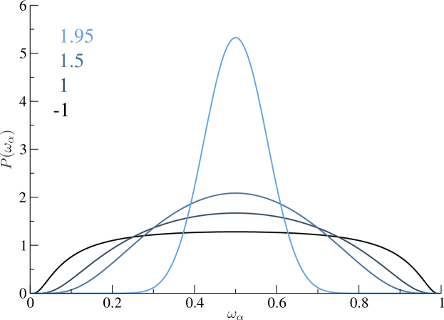
Figure 5: (color online) The distribution $P(\omega_{\alpha})$ in Eq. (7.11) for different $\alpha<2$ in 2D systems.

In Fig. 5 we plot the distribution in Eq. 7.11 for different values of $\alpha<2$. One notices that similarly to the 3D case, as $\alpha\to 2$ the distribution becomes progressively narrower and the peak at $\omega=1/2$ becomes more pronounced, which means that it becomes progressively more likely that the diffusion coefficients, deduced from two different realisations of Brownian trajectories using the weighted least-squares estimators, will have the same value. One notices as well that for the unweighted LSE ($\alpha=1$), the distribution $P(\omega)$ is rather flat, pointing at large discrepancies between the estimates obtained from different trajectories.

8 Conclusions

To conclude, we have studied the distribution function $P(u_{\alpha})$ of the estimators $u_{\alpha}\sim T^{-1}\int^{T}_{0}\,\omega(t)\,{\bf B}^{2}_{t}\,dt$, which optimise the least-squares fitting of the diffusion coefficient $D_{f}$ of a single $d$-dimensional Brownian trajectory ${\bf B}_{t}$. We pursued here the optimisation further by considering a family of weight functions of the form $\omega(t)=(t_{0}+t)^{-\alpha}$, where $t_{0}$ is a time lag and $\alpha$ is an arbitrary real number, and seeking such values of $\alpha$ for which the estimators most efficiently filter out the fluctuations. We calculated $P(u_{\alpha})$ exactly for arbitrary $\alpha$ and for arbitrary spatial dimension $d$, and showed that only for $\alpha=2$ the distribution $P(u_{\alpha})$ converges, as $\epsilon=t_{0}/T\to 0$, to the Dirac delta-function centered at the ensemble average value of the estimator. This allowed us to conclude that only the estimators with $\alpha=2$ possess an ergodic property, so that the ensemble averaged diffusion coefficient can be obtained with any necessary precision from a single trajectory data, but at the expense of a progressively higher experimental resolution. For any $\alpha\neq 2$ the distribution attains, as $\epsilon\to 0$, a certain limiting form with a finite variance, which signifies that such estimators are not ergodic.

References

References

- [1] Perrin J, 1908 C. R. Acad. Sci. 146 967; 1909 Ann. Chim. Phys. 18 5.
- [2] Bräuchle C, Lamb D C and Michaelis J, Eds., 2010 Single particle tracking and single molecule energy transfer (Wiley-VCH, Weinheim).
- [3] Saxton M J and Jacobson K, 1977 Ann. Rev. Biophys. Biomol. Struct. 26 373.
- [4] Mason T G and Weitz D A, 1995 Phys. Rev. Lett. 74 1250.
- [5] Greenleaf W J, Woodside M T and Block S M, 2007 Annu. Rev. Biophys. Biomol. Struct. 36 171.
- [6] Golding I and Cox E C, 2006 Phys. Rev. Lett. 96 098102.
- [7] Weber S C, Spakowitz A J and Theriot J A, 2010 Phys. Rev. Lett. 104 238102.
- [8] Bronstein I et al., 2009 Phys. Rev. Lett. 103 018102.
- [9] Seisenberger G et al., 2001 Science 294 1929.
- [10] Weigel A V, Simon B, Tamkun M M and Krapf D, 2011 Proc. Natl. Acad. Sci. USA 108 6438.
- [11] Moerner W E, 2007 Proc. Natl. Acad. Sci. USA 104 12596.
- [12] Rebenshtok A and Barkai E, 2007 Phys. Rev. Lett. 99 210601.
- [13] Jeon J H et al., 2011 Phys. Rev. Lett. 106 048103.
- [14] He Y, Burov S, Metzler R and Barkai E, 2008 Phys. Rev. Lett. 101 058101.
- [15] Lubelski A, Sokolov I M and Klafter J, 2008 Phys. Rev. Lett. 100 250602.
- [16] Schulz J, Barkai E and Metzler R, Ageing effects in single particle trajectory averages, arXiv:1204.0878v1
- [17] Mejía-Monasterio C, Oshanin G and Schehr G, 2011 J. Stat. Mech. P06022.
- [18] Mattos T G, Mejía-Monasterio C, Metzler R and Oshanin G, 2012 Phys. Rev. E 86 031143.
- [19] Wang Y M, Austin R H and Cox E C, 2006 Phys. Rev. Lett. 97 048302.
- [20] Goulian M and Simon S M, 2000 Biophys. J. 79 2188.
- [21] Saxton M J, 1997 Biophys. J. 72 1744.
- [22] Grebenkov D S, 2011 Phys. Rev. E 83 061117.
- [23] Grebenkov D S, 2011 Phys. Rev. E 84 031124.
- [24] Andreanov A and Grebenkov D S, J. Stat. Mech. (2012) P07001
- [25] Tejedor V et al., 2010 Biophys J 98 1364.
- [26] Berglund A J, 2010 Phys. Rev. E 82 011917.
- [27] Michalet X, 2010 Phys. Rev. E 82 041914; 2011 83 059904.
- [28] Michalet X and Berglund A J, 2012 Phys. Rev. E 85 061916.
- [29] Boyer D and Dean D S, 2011 J. Phys. A: Math. Gen. 44 335003.
- [30] Boyer D, Dean D S, Mejía-Monasterio C and Oshanin G, 2012 Phys. Rev. E 85 031136.
- [31] Boyer D, Dean D S, Mejía-Monasterio C and Oshanin G, Optimal fits of diffusion constants from single time data points of Brownian trajectories, arXiv:1211.1151
- [32] Eliazar I, 2005 Physica A 356 207.
- [33] Eliazar I and Sokolov I M, 2010 Journal of Physics A: Mathematical and Theoretical 43 055001.
- [34] Eliazar I and Sokolov I M, 2012 Physica A 391 3043.
- [35] Cameron R H and Martin W T, 1945 Bull. Am. Math. Soc. 51 73.
- [36] Kac M, 1949 Trans. Am. Math. Soc. 65 1.
- [37] Rogers L C G and Shi Z, 1992 Stochastics Stochastics Rep. 41 201.
- [38] Donati-Martin C and Yor M, 1993 Adv. Appl. Prob. 25 570.
- [39] Kleptsyna M L and Le Breton A, 2002 Stochastics 72 229.
- [40] Feynman R P and Hibbs A R, 1965 Quantum Mechanics and Path Integrals (New York: McGraw-Hill)
- [41] Kleinert H, 2006 Path Integrals in Quantum Mechanics, Statistics, Polymer Physics and Financial Markets (Singapore: World Scientific)
- [42] Khandekar D C and Lawande S V, 1986 Phys. Rep. 137 115.
- [43] Dean D S and Jansons K M, 1995 J. Stat. Phys. 79 265.
- [44] Dean D S and Horgan R R, 2005 J. Phys.: Condens. Matter 17 3473.
- [45] Parsegian V A, 2006 Van der Waals Forces (Cambridge: Cambridge University Press)
- [46] Dean D S and Horgan R R, 2007 Phys. Rev. E 76 041102.
- [47] Dean D S, Horgan R R, Naji A and Podgornik R, 2009 Phys. Rev. A 79 040101.
- [48] Dean D S, Horgan R R, Naji A and Podgornik R, 2010 Phys. Rev. E 81 051117.
- [49] Attard P, Mitchell J and Ninham B W, 1998 J. Chem. Phys. 88 4987.
- [50] Podgornik R and Zeks T, 1998 J. Chem. Soc. Faraday Trans. 2 84 611.
- [51] Podgornik R, 1990 J. Phys. A: Math. Gen. 23 275.
- [52] Dean D S, Horgan R R, Naji A and Podgornik R, 2009 J. Chem. Phys. 130 094504.
- [53] Majumdar S N, 2005 Curr. Sci. 89 2076.
- [54] Abramowitz M and Stegun I R, Eds., 1972 Handbook of mathematical functions (Dover, New York).
- [55] Mejía-Monasterio C, Oshanin G and Schehr G, 2011 Phys. Rev. E 84 035203.
- [56] Oshanin G, Wio H S, Lindenberg K and Burlatsky S F, 2007 J. Phys.: Condens. Matter 19, 065142.
- [57] Oshanin G, Lindenberg K, Wio H S and Burlatsky S F, 2009 J. Phys. A: Math. Theor. 42, 434008.