On the theory of superconductivity in the extended Hubbard model:
Spin-fluctuation pairing

Abstract

A microscopic theory of superconductivity in the extended Hubbard model which takes into account the intersite Coulomb repulsion and electron-phonon interaction is developed in the limit of strong correlations. The Dyson equation for normal and pair Green functions expressed in terms of the Hubbard operators is derived. The self-energy is obtained in the noncrossing approximation. In the normal state, antiferromagnetic short-range correlations result in the electronic spectrum with a narrow bandwidth. We calculate superconducting $T_{c}$ by taking into account the pairing mediated by charge and spin fluctuations and phonons. We found the $d$-wave pairing with high-$T_{c}$ mediated by spin fluctuations induced by the strong kinematic interaction for the Hubbard operators. Contributions to the $d$-wave pairing coming from the intersite Coulomb repulsion and phonons turned out to be small.

I Introduction

Despite intensive studies of high-temperature superconductivity (HTSC) in cuprates for many years after the discovery of Bednorz and Müller Bednorz86 , a commonly accepted mechanism of HTSC is still lacking (see, e.g. Schrieffer07 ; Plakida10 ). A good candidate from various proposed mechanisms is based on a model of strongly correlated electrons Anderson87 . In the model, superconductivity occurs at finite doping in the resonating valence bond state (RVB) due to the antiferromagnetic (AF) superexchange in the $t$–$J$ model. A possibility of HTSC mediated by AF spin fluctuations as a “glue” for superconducting pairing was also considered Scalapino95 , mostly within phenomenological spin-fermion models (see, e.g., Monthoux94b ; Moriya00 ; Chubukov04 ; Abanov08 , and references therein).

Recent studies of spin-excitations by magnetic inelastic neutron scattering (INS) and the electronic spectrum by angle-resolved photoemission spectroscopy (ARPES) have revealed an important role of AF spin excitations in the “kink” phenomenon and the $d$-wave pairing in cuprates (see, e.g., Kordyuk10 and references therein). In particular, in Ref. Dahm09 using INS and ARPES studies on the same YBa₂Cu₃O_6.6 (YBCO_6.6) crystal, an estimation for superconducting $T_{c}\sim 150$ K was found. The main argument against the spin-fluctuation pairing, the weak intensity of spin fluctuations at the optimal doping seen in INS experiments Bourges98 , was dismissed in the recent resonant inelastic x-ray scattering experiments LeTacon11 . In a large family of cuprate superconductors, paramagnon AF excitations with the dispersion and spectral weight similar to those of magnons in undoped cuprates were observed. Using the magnetic spectrum found in the YBCO₇ crystal, superconductivity with $T_{c}=100-200$ K was predicted. Thus, spin fluctuations have sufficient strength to mediate HTSC in cuprates and to explain various physical properties of cuprate materials as, e.g., the optical conductivity Vladimirov12 . Therefore, it can be suggested that the alternative mechanism based on the conventional electron-phonon interaction (EPI) (see, e.g., Kulic04 ; Maksimov10 ) plays a secondary role in the cuprate superconductors.

Recently, in Ref. Raghu10 using the renormalization group (RG) method an asymptotically exact solution for the $d$-wave pairing was found in the conventional Hubbard model Hubbard63 in the weak correlation limit, $U\ll t$. However, as was pointed out later in Ref. Alexandrov11 , a contribution from the repulsive well-screened weak Coulomb interaction (CI) in the first order strongly suppresses the pairing induced by the contributions of higher orders, and a possibility for superconductivity “from repulsion” was questioned. At the same time, in Ref. KaganM11 it was shown that the $p$-wave superconductivity exists in the electronic gas at low density with a strong repulsion $U$ and a relatively strong Coulomb intersite interaction $V_{ij}$ (see, also Efremov00 and references therein). Later on, in Ref. Raghu12 RG studies of the extended Hubbard model with the intersite interaction have shown that superconducting pairing of various symmetries, extended $s$-, $p$-, and $d$-wave types, can occur depending on the electron concentration and the intersite interaction $V_{ij}$. However, in these investigations the Fermi-liquid model in the weak correlation limit was used. To study superconductivity in cuprates, the Mott-Hubbard (more accurately, charge-transfer) doped insulators, a theory of strongly correlated electronic systems should be used (for reviews see Fulde95 ; Avella11 ).

In the present paper we consider superconductivity in the extended Hubbard model with a weak intersite Coulomb repulsion $V_{ij}$ but in comparison with Refs. Raghu10 ; Alexandrov11 ; Raghu12 , we study the limit of strong correlations, $U\gg t$. To compare various contributions to the superconducting $d$-wave pairing, we consider also a model of the EPI with strong forward scattering proposed in Ref. Zeyher96 . The Dyson equation for the thermodynamic Green functions (GFs) expressed in terms of the Hubbard operators (HOs) is derived using the Mori-type projection technique Mori65 . The self-energy is calculated in the noncrossing approximation (NCA) as in the microscopic theory of the electronic spectrum in the normal state in our previous publication Plakida07 . We show that the kinematic interaction for the HOs generates the AF superexchange pairing similar to the $t$–$J$ model. A contribution from the intersite Coulomb repulsion in the first order suppresses the pairing as found in Refs. Alexandrov11 ; Raghu12 . But the kinematic interaction induces also a strong electron interaction with spin-fluctuations which results in the $d$-wave superconductivity with high-$T_{c}$. Contribution from the EPI to the d-wave pairing turned out to be small.

In the next section we introduce the model, derive the Dyson equation, and calculate the self-energy in the NCA. A self-consistent system of equations is formulated in Sec. III. Results of computations of the electronic spectrum in the normal state and of superconducting $T_{\rm c}$ and the $d$-wave gap function are presented in Sec. IV. Concluding remarks are given in Sec. V. In the Appendix details of the calculations are given.

II General formulation

II.1 Extended Hubbard model

We consider an extended Hubbard model on a square lattice which we write in terms of the HOs Hubbard65 :

$$H=\varepsilon_{1}\sum_{i,\sigma}X_{i}^{\sigma\sigma}+\varepsilon_{2}\sum_{i}X_{i}^{22}+\sum_{i\neq j,\sigma}\bigl{\{}t_{ij}^{11}X_{i}^{\sigma 0}X_{j}^{0\sigma}$$

$$+t_{ij}^{22}X_{i}^{2\sigma}X_{j}^{\sigma 2}+\sigma t_{ij}^{12}(X_{i}^{2\bar{\sigma}}X_{j}^{0\sigma}+{\rm H.c.})\bigr{\}}+H_{c,ep}.$$ (1)

To apply the model for consideration of the cuprate superconductors, we introduce the HOs for holes taking into account four possible states on a lattice site $i$: an empty state $(\alpha,\beta=0)$, a singly occupied hole state $(\alpha,\beta=\sigma)$ with the spin $\sigma/2=\pm(1/2)\,,\;\bar{\sigma}=-\sigma$, and a two-hole state $(\alpha,\beta=2)$. Then the HO $X_{i}^{\alpha\beta}=|i\alpha\rangle\langle i\beta|$ describes the transition from the state $|i,\beta\rangle$ to the state $|i,\alpha\rangle$. Energy parameters in the model (1) are taken close to the values found within the cell-perturbation method Feiner96 for the $p$-$d$ model for the CuO₂ plane Emery87 . In particular, the single-particle energy $\varepsilon_{1}=\varepsilon_{d}-\mu$ is the energy of the $d$-type one-hole state measured from the chemical potential $\mu$ and the two-particle energy $\varepsilon_{2}=2\varepsilon_{1}+U$ is the energy of the two-hole $p$-$d$ Zhang-Rice singlet state Zhang88 . The effective Hubbard $U$ in cuprates is the charge-transfer energy $U=\Delta_{pd}=\epsilon_{p}-\epsilon_{d}$. According to the cell perturbation method, in general case the values of the hopping parameters $t^{\eta\zeta}_{ij}$ in (1) depends on the the subband indices $\eta,\zeta=1,\,2$.

In the last term in (1) in addition to the inertsite CI $V_{ij}$ for holes in the plane we take into account also the EPI $g_{ij}$ for holes with phonons:

$$H_{c,ep} = \frac{1}{2}\sum_{i\neq j}\,V_{ij}N_{i}N_{j}+\sum_{i,j}\,g_{ij}N_{i}\,u_{j},$$ (2)

where $u_{j}$ describes an atomic displacement on the lattice site $j$ for a particular phonon mode. More generally, the EPI can be written as a sum $\sum_{\nu}g^{\nu}_{i,j}u_{j}^{\nu}$ over the normal modes $\nu$. The hole number operator and the spin operators in terms of HOs are defined as

$$N_{i} = \sum_{\sigma}X_{i}^{\sigma\sigma}+2X_{i}^{22},$$ (3)

$$S_{i}^{\sigma} = X_{i}^{\sigma\bar{\sigma}},\quad S_{i}^{z}=(\sigma/2)\,[X_{i}^{\sigma\sigma}-X_{i}^{\bar{\sigma}\bar{\sigma}}].$$ (4)

The completeness relation for the HOs, $\,X_{i}^{00}+\sum_{\sigma}X_{i}^{\sigma\sigma}+X_{i}^{22}=1$, rigorously preserves the constraint of no double occupancy of the quantum state $\alpha$ on any lattice site $i$. From the multiplication rule $\,X_{i}^{\alpha\beta}X_{i}^{\gamma\delta}=\delta_{\beta\gamma}X_{i}^{\alpha\delta}\,$ follows the commutation relations:

$$\left[X_{i}^{\alpha\beta},X_{j}^{\gamma\delta}\right]_{\pm}=\delta_{ij}\left(\delta_{\beta\gamma}X_{i}^{\alpha\delta}\pm\delta_{\delta\alpha}X_{i}^{\gamma\beta}\right)\,.$$ (5)

The upper sign refers to the Fermi-type operators like $X_{i}^{0\sigma}$ while the lower sign refers to the Bose-type operators like $N_{i}$ (3) or the spin operators (4).

The chemical potential $\mu$ depends on the average hole occupation number

$$n=1+\delta=\langle\,N_{i}\rangle,$$ (6)

where $\langle...\rangle$ denotes the statistical average with the Hamiltonian (1).

We emphasize here that the Hubbard model (1) does not involve a dynamical coupling of electrons (holes) to fluctuations of spins or charges. Its role is played by the kinematic interaction caused by the complicated commutation relations (5), as was already noted by Hubbard Hubbard65 . For example, the equation of motion for the HO $\,X_{i}^{\sigma 2}\,$ in the Heisenberg representation $(\hbar=1)$ reads,

$$i\frac{d}{dt}X_{i}^{\sigma 2} = [X_{i}^{\sigma 2},H]=(\varepsilon_{1}+U)\,X_{i}^{\sigma 2}\,$$ (7)

$$+ \sum_{l,\sigma^{\prime}}\!\left(t_{il}^{22}B_{i\sigma\sigma^{\prime}}^{22}X_{l}^{\sigma^{\prime}2}-\sigma t^{21}_{il}B_{i\sigma\sigma^{\prime}}^{21}X_{l}^{0\bar{\sigma}^{\prime}}\right)$$

$$- \sum_{l}X_{i}^{02}\left(t^{11}_{il}X_{l}^{\sigma 0}+\sigma t^{21}_{il}X_{l}^{2\bar{\sigma}}\right)$$

$$+ \sum_{l}X_{i}^{\sigma 2}(V_{il}\,N_{l}+g_{il}\,u_{l}).$$

Here $B_{i\sigma\sigma^{\prime}}^{\eta\zeta}$ are the Bose-like operators,

$$B_{i\sigma\sigma^{\prime}}^{22} = (X_{i}^{22}+X_{i}^{\sigma\sigma})\,\delta_{\sigma^{\prime}\sigma}+X_{i}^{\sigma\bar{\sigma}}\,\delta_{\sigma^{\prime}\bar{\sigma}}$$

$$= (N_{i}/2+\sigma\,S_{i}^{z})\,\delta_{\sigma^{\prime}\sigma}+S_{i}^{\sigma}\,\delta_{\sigma^{\prime}\bar{\sigma}},$$

$$B_{i\sigma\sigma^{\prime}}^{21} = (N_{i}/2+\sigma S_{i}^{z})\,\delta_{\sigma^{\prime}\sigma}-S_{i}^{\sigma}\,\delta_{\sigma^{\prime}\bar{\sigma}},$$ (9)

where we used the definition of the number operator (3) and the spin operators (4). The last term in (7) is caused by the dynamic intersite CI and the EPI.

II.2 Dyson equation

To consider the superconducting pairing in the model (1), we introduce the two-time thermodynamic GF Zubarev60 expressed in terms of the four-component Nambu operators, $\,\hat{X}_{i\sigma}$ and $\,\hat{X}_{i\sigma}^{\dagger}=(X_{i}^{2\sigma}\,\,X_{i}^{\bar{\sigma}0}\,\,X_{i}^{\bar{\sigma}2}\,\,X_{i}^{0\sigma})\,$:

$${\sf G}_{ij\sigma}(t-t^{\prime}) = -i\theta(t-t^{\prime})\langle\{\hat{X}_{i\sigma}(t),\hat{X}_{j\sigma}^{\dagger}(t^{\prime})\}\rangle$$ (10)

$$\equiv \langle\!\langle\hat{X}_{i\sigma}(t)\mid\hat{X}_{j\sigma}^{\dagger}(t^{\prime})\rangle\!\rangle,$$

where $\{A,B\}=AB+BA$, $A(t)=\exp(iHt)A\exp(-iHt)$, and $\theta(x)=1$ for $x>0$ and $\theta(x)=0$ for $x<0$. The Fourier representation in $({\bf k},\omega)$-space is defined by the relations:

$${\sf G}_{ij\sigma}(t-t^{\prime}) = \frac{1}{2\pi}\int_{-\infty}^{\infty}dte^{-i(t-t^{\prime})}{\sf G}_{ij\sigma}(\omega),$$ (11)

$${\sf G}_{ij\sigma}(\omega) = \frac{1}{N}\,\sum_{\bf k}\exp[i{\bf k(i-j)}]{\sf G}_{\sigma}({\bf k},\omega).$$ (12)

The GF (11) is convenient to write in the matrix form

$${\sf G}_{ij\sigma}(\omega)={\hat{G}_{ij\sigma}(\omega)\quad\quad\hat{F}_{ij\sigma}(\omega)\choose\hat{F}_{ij\sigma}^{\dagger}(\omega)\quad-\hat{G}_{ji\bar{\sigma}}(-\omega)},$$ (13)

where the normal $\hat{G}_{ij\sigma}$ and anomalous (pair) $\hat{F}_{ij\sigma}$ GFs are the $2\times 2$ matrices for two Hubbard subbands:

$$\hat{G}_{ij}(\omega)=\langle\!\langle\left(\begin{array}[]{c}X_{i}^{\sigma 2}\\ X_{i}^{0\bar{\sigma}}\\ \end{array}\right)\mid X_{j}^{2\sigma}X_{j}^{\bar{\sigma}0}\rangle\!\rangle_{\omega},$$ (14)

$$\hat{F}_{ij}(\omega)=\langle\!\langle\left(\begin{array}[]{c}X_{i}^{\sigma 2}\\ X_{i}^{0\bar{\sigma}}\\ \end{array}\right)\mid X_{j}^{\bar{\sigma}2}X_{j}^{0\sigma}\rangle\!\rangle_{\omega}.$$ (15)

To calculate the GF (10) we use the equation of motion method. Differentiating the GF with respect to time $t$, the Fourier representation of it leads to the equation

$$\omega{\sf G}_{ij\sigma}(\omega)=\delta_{ij}{\sf Q}+\langle\!\langle[\hat{X}_{i\sigma},H]\mid\hat{X}_{j\sigma}^{\dagger}\rangle\!\rangle_{\omega}\,.$$ (16)

Here the correlation function ${\sf Q}=\langle\{\hat{X}_{i\sigma},\hat{X}_{i\sigma}^{\dagger}\}\rangle=\hat{\tau}_{0}\times\hat{Q}\,$ where $\,\hat{Q}=\left(\begin{array}[]{cc}Q_{2}&0\\ 0&Q_{1}\end{array}\right)\,$ and $\hat{\tau}_{0}$ is the $2\times 2$ unit matrix. The spectral weights of the Hubbard subbands in the paramagnetic state $\,Q_{2}=\langle X_{i}^{22}+X_{i}^{\sigma\sigma}\rangle=n/2\,$ and $\,Q_{1}=\langle X_{i}^{00}+X_{i}^{\bar{\sigma}\bar{\sigma}}\rangle=1-Q_{2}\,$ depend on the occupation number of holes (6). In the $\,{\sf Q}$ matrix we neglect anomalous averages of the type $\langle X_{i}^{02}\rangle$ which are irrelevant for the $d$-wave pairing Adam07 .

To introduce the zero-order quasiparticle (QP) excitation energy we use the Mori-type projection method Mori65 . In this approach, the many-particle operator $\hat{Z}_{i\sigma}=[\hat{X}_{i\sigma},H]$ in (16) is written as a sum of a linear part and an irreducible part $\hat{Z}_{i\sigma}^{(ir)}$ orthogonal to $\hat{X}_{j\sigma}^{\dagger}$:

$$\hat{Z}_{i\sigma}=[\hat{X}_{i\sigma},H]=\sum_{l}{\sf E}_{il\sigma}\hat{X}_{l\sigma}+\hat{Z}_{i\sigma}^{(\rm ir)}.$$ (17)

The orthogonality condition $\langle\{\hat{Z}_{i\sigma}^{(\rm ir)},\,\hat{X}_{j\sigma}^{\dagger}\}\rangle=0\,$ determines the excitation energy in the mean-field approximation (MFA)

$${\sf E}_{ij\sigma} = \langle\{[\hat{X}_{i\sigma},H],\hat{X}_{j\sigma}^{\dagger}\}\rangle{\sf Q}^{-1}$$ (18)

$$= (1/N)\,\sum_{\bf k}\exp[i{\bf k(i-j)}]\,{\sf E}_{\sigma}({\bf k}),$$

and the corresponding zero-order GF

$${\sf G}^{0}_{\sigma}({\bf k},\omega)=\Bigl{(}\omega\tilde{\tau}_{0}-{\sf E}_{\sigma}({\bf k})\Bigr{)}^{-1}{\sf Q}\,,$$ (19)

where $\tilde{\tau}_{0}$ is the $4\times 4$ unit matrix.

To calculate the multiparticle GF $\,\langle\langle\hat{Z}_{i\sigma}^{(\rm ir)}(t)\mid\hat{X}_{j\sigma}^{\dagger}(t^{\prime})\rangle\rangle\,$ in (16) we differentiate it with respect to the second time $t^{\prime}$ and apply the same projection procedure as in (17). This results in the equation for the GF (16) in the form,

$${\sf G}_{\sigma}({\bf k},\omega)={\sf G}^{0}_{\sigma}({\bf k},\omega)+{\sf G}^{0}_{\sigma}({\bf k},\omega)\,{\sf T}_{\sigma}({\bf k},\omega)\,{\sf G}^{0}_{\sigma}({\bf k},\omega),$$ (20)

where the scattering matrix

$${\sf T}_{\sigma}({\bf k},\omega)={\sf Q}^{-1}\,\langle\!\langle{\hat{Z}}_{{\bf k}\sigma}^{(\rm ir)}\!\mid\!{\hat{Z}}_{{\bf k}\sigma}^{(\rm ir)\dagger}\rangle\!\rangle_{\omega}\;{\sf Q}^{-1}.$$ (21)

Now we can introduce the self-energy operator ${\sf\Sigma}_{\sigma}({\bf q},\omega)$ as the proper part (pp) of the scattering matrix (21) which has no parts connected by the zero-order GF (19) according to the equation: ${\sf T}={\sf\Sigma}+{\sf\Sigma}\,{\sf G}^{0}\,{\sf T}$. The definition of the proper part of the scattering matrix (21) is equivalent to an introduction of a projected Liouvillian superoperator for the memory function in the conventional Mori technique Mori65 .

Using the self-energy operator instead of the scattering matrix in Eq. (20) we obtain the Dyson equation for the GF (10):

$${\sf G}_{\sigma}({\bf k},\omega)=\left[\omega\tilde{\tau}_{0}-{\sf E}_{\sigma}({\bf k})-{\sf Q}{\sf\Sigma}_{\sigma}({\bf k},\omega)\right]^{-1}{\sf Q},$$ (22)

where the self-energy operator is given by

$${\sf Q}{\sf\Sigma}_{\sigma}({\bf k},\omega)=\langle\!\langle{\hat{Z}}_{{\bf k}\sigma}^{(\rm ir)}\!\mid\!{\hat{Z}}_{{\bf k}\sigma}^{(\rm ir)\dagger}\rangle\!\rangle^{(\rm pp)}_{\omega}\;{\sf Q}^{-1}.$$ (23)

Dyson equation (22) with the zero-order QP excitation energy (18) and the self-energy (23) gives an exact representation for the GF (10). The self-energy takes into account processes of inelastic scattering of electrons (holes) on spin and charge fluctuations due to the kinematic interaction and the dynamic intersite CI and the EPI (see Eq. (7)). To obtain a closed system of equations, the multiparticle GF in the self-energy operator (23) should be evaluated as discussed below.

III Self-consistent system of equations

III.1 Mean-field approximation

The superconducting pairing in the Hubbard model already occurs in the MFA and is caused by the kinetic superexchange interaction as in the $t$–$J$ model Anderson87 . Therefore, it is reasonable to consider at first the MFA described by the zero-order GF (19). Using commutation relations (5) for the HOs we calculate the energy matrix (18):

$${\sf E}_{ij\sigma}=\left(\begin{array}[]{cc}\hat{\varepsilon}_{ij}&\hat{\Delta}_{ij\sigma}\\ \hat{\Delta}_{ji\sigma}^{*}&-\hat{\varepsilon}_{ji\bar{\sigma}}\end{array}\right).$$ (24)

The matrix $\hat{\varepsilon}({\bf k})=\sum_{j}\,\exp[i{\bf k}({\bf i-j})]\,\hat{\varepsilon}_{ij}$ after diagonalization determines the QP spectrum in the two Hubbard subbands in the normal state (for details see Plakida07 ):

$${\varepsilon}_{1,2}({\bf k}) = ({1}/{2})[\omega_{2}({\bf k})+\omega_{1}({\bf k})]\mp({1}/{2})\Lambda({\bf k}),$$ (25)

$${\omega}_{\iota}({\bf k}) = 4t\,\alpha_{\iota}\gamma({\bf k})+4\,\beta_{\iota}\,t^{\prime}\gamma^{\prime}({\bf k})+4\,\beta_{\iota}\,t^{\prime\prime}\gamma^{\prime\prime}({\bf k})$$ (26)

$$+ \omega^{(c)}_{\iota}({\bf k})+U\delta_{\iota,2}-\mu,\quad(\iota=1,2)$$

$$\Lambda({\bf k}) = \{[\omega_{2}({\bf k})-\omega_{1}({\bf k})]^{2}+4W({\bf k})^{2}\}^{1/2},$$

$$W({\bf k}) = 4t\,\alpha_{12}\gamma({\bf k})+4t^{\prime}\,\beta_{12}\gamma^{\prime}({\bf k})+4t^{\prime\prime}\,\beta_{12}\gamma^{\prime\prime}({\bf k}).$$

Here the hopping parameters in (1) are assumed to be equal, $\,t^{22}_{ij}=t^{11}_{ij}=t^{12}_{ij}=t_{ij}$, where $t_{ij}$ is defined by the expression:

$$t_{ij} = (1/N)\,\sum_{\bf k}\exp[i{\bf k(i-j)}]\,t({\bf k}),$$ (27)

$$t({\bf k}) = 4t\,\gamma({\bf k})+4t^{\prime}\,\gamma^{\prime}({\bf k})+4t^{\prime\prime}\,\gamma^{\prime\prime}({\bf k}).$$ (28)

The hopping parameters are equal to $t\,$ for the nearest neighbor (n.n.) sites $a_{1}=(\pm a_{x},\pm a_{y})$, $\,t^{\prime}\,$ – for the next nearest neighbor (n.n.n.) sites $a_{d}=\pm(a_{x}\pm a_{y})$, and $\,t^{\prime\prime}\,$ – for the n.n.n. sites $\,a_{2}=\pm 2a_{x},\pm 2a_{y}$. The corresponding ${\bf k}$-dependent functions are: $\,\gamma({\bf k})=(1/2)(\cos k_{x}+\cos k_{y}),\;\gamma^{\prime}({\bf k})=\,\cos k_{x}\cos k_{y}\,$, and $\;\gamma^{\prime\prime}({\bf k})=(1/2)(\cos 2k_{x}+\cos 2k_{y})$ (the lattice constants $a_{x}=a_{y}$ are put to unity). The contribution from the CI $V_{ij}$ in (26) is given by

$$\omega^{(c)}_{1(2)}({\bf k})=\frac{1}{N}\sum_{\bf q}V({\bf k-q})N_{1(2)}({\bf q}),$$ (29)

where $N_{1}({\bf q})=\langle X_{\bf q}^{0\bar{\sigma}}X_{\bf q}^{\bar{\sigma}0}\rangle/Q_{1},\;N_{2}({\bf q})=\langle X_{\bf q}^{\sigma 2}X_{{}_{\bf q}}^{2\sigma}\rangle/Q_{2}$ and $V({\bf k-q})$ is the Fourier transform of $V_{ij}$.

The kinematic interaction for the HOs results in renormalization of the spectrum (25) determined by the parameters: $\,\alpha_{\iota}=Q_{\iota}[1+{C_{1}}/{Q^{2}_{\iota}}],\,\beta_{\iota}=Q_{\iota}[1+{C_{2}}/{Q^{2}_{\iota}}]\,$, $\,\alpha_{12}=\sqrt{Q_{1}Q_{2}}[1-{C_{1}}/{Q_{1}Q_{2}}],\,\beta_{12}=\sqrt{Q_{1}Q_{2}}[1-{C_{2}}/{Q_{1}Q_{2}}]\,$. Here we take into account the renormalization caused by the spin correlation functions for the n.n. and the n.n.n. sites, respectively:

$$C_{1}=\langle{\bf S}_{i}{\bf S}_{i+a_{1}}\rangle,\quad C_{2}=\langle{\bf S}_{i}{\bf S}_{i+a_{d}}\rangle\approx\langle{\bf S}_{i}{\bf S}_{i+a_{2}}\rangle.$$ (30)

The short-range AF correlations considerably suppress the n.n. hopping parameters since $C_{1}<0\,$ and at low doping $\,|C_{1}|=0.1-0.2$ that results in $\alpha_{\iota}\ll 1$. At the same time, the n.n.n. hopping parameters are increased since $C_{2}>0$.

Now we evaluate the anomalous components $\hat{\Delta}_{ij\sigma}$ of the matrix (24) which determine the superconducting gap in the MFA. Considering the singlet $d$-wave pairing, we calculate the intersite pair correlation functions. The diagonal matrix components are given by the equations:

$$\Delta_{ij\sigma}^{22}Q_{2}=-\sigma\,t_{ij}^{21}\langle X_{i}^{02}N_{j}\rangle-V_{ij}\langle X_{i}^{\sigma 2}\,X_{j}^{\bar{\sigma}2}\rangle,$$ (31)

$$\Delta_{ij\sigma}^{11}Q_{1}=\sigma\,t_{ij}^{12}\langle N_{j}X_{i}^{02}\rangle-V_{ij}\langle X_{i}^{0\bar{\sigma}}X_{j}^{0\sigma}\rangle.$$ (32)

Here we used the original notation for the interband hopping parameters $t_{ij}^{12}$ to emphasize that the kinematic pairing $\langle X_{i}^{02}N_{j}\rangle$ is mediated by the interband hopping. In terms of the Fermi operators $a_{i\sigma}=X_{i}^{0\sigma}+\sigma X_{i}^{\bar{\sigma}2}$, the pair correlation function in (31) can be written as $\,\langle X_{i}^{02}N_{j}\rangle=\langle X_{i}^{0\downarrow}X_{i}^{\downarrow 2}N_{j}\rangle=\langle a_{i\downarrow}\,a_{i\uparrow}N_{j}\rangle$. This representation shows that the kinematic pairing occurs on a single lattice site but in two Hubbard subbands Plakida03 .

The correlation function $\,\langle X_{i}^{02}N_{j}\rangle$ can be calculated directly from the GF $\,L_{ij}(t-t^{\prime})=\langle\langle X_{i}^{02}(t)\mid N_{j}(t^{\prime})\rangle\rangle\,$ without any decoupling approximation as shown in Ref. Plakida03 . In particular, under hole doping, $n=1+\delta>1$, the pair correlation function in the two-site approximation reads (for details see Appendix A):

$$\langle X_{i}^{02}N_{j}\rangle=-\frac{4t_{ij}^{12}}{U}\sigma\,\langle X_{i}^{\sigma 2}X_{j}^{\bar{\sigma}2}\rangle.$$ (33)

As a result, the equation for the superconducting gap in (31) can be written as

$$\Delta^{22}_{ij\sigma}=(J_{ij}-V_{ij})\,\langle X_{i}^{\sigma 2}X_{j}^{\bar{\sigma}2}\rangle/Q_{2},$$ (34)

where $\,J_{ij}={4\,(t_{ij}^{12})^{2}}/{U}$ is the AF superexchange interaction. A similar equation holds for the gap in the one-hole subband: $\,\Delta_{ij\sigma}^{11}=(J_{ij}-V_{ij})\,\langle X_{i}^{0\bar{\sigma}}X_{j}^{0\sigma}\rangle/Q_{1}\,$. We thus conclude that the pairing in the Hubbard model in the MFA is similar to the superconductivity in the $t$–$J$ model mediated by the AF superexchange interaction $J_{ij}$.

III.2 Self-energy operator

Self-energy operator (23) can be written in the same matrix form as the GF (13):

$${\sf Q}\,{\sf\Sigma}_{ij\sigma}(\omega)={\hat{M}_{ij\sigma}(\omega)\quad\quad\hat{\Phi}_{ij\sigma}(\omega)\choose\hat{\Phi}_{ij\sigma}^{\dagger}(\omega)\quad-\hat{M}_{ji\bar{\sigma}}(-\omega)}{\sf Q}^{-1}\,,$$ (35)

where the matrices $\hat{M}$ and $\hat{\Phi}$ denote the respective normal and anomalous (pair) components of the self-energy operator. The system of equations for the $(4\times 4)$ matrix GF (13) and the self-energy (35) can be reduced to a system of equations for the normal ${\hat{G}}_{\sigma}({\bf k},\omega)$ and the pair ${\hat{F}}_{\sigma}({\bf k},\omega)$ $(2\times 2)$ matrix components. Using representations for the energy matrix (24) and the self-energy (35), we derive for these components the following system of matrix equations:

$${\hat{G}}({\bf k},\omega) = \Bigl{(}\hat{G}_{N}({\bf k},\omega)^{-1}$$ (36)

$$+ \hat{\varphi}_{\sigma}({\bf k},\omega)\,\hat{G}_{N}({\bf k},-\omega)\,\hat{\varphi}^{*}_{\sigma}({\bf k},\omega)\Bigr{)}^{-1}\,\hat{Q},\qquad$$

$${\hat{F}}_{\sigma}({\bf k},\omega) = -\hat{G}_{N}({\bf k},-\omega)\,\hat{\varphi}_{\sigma}({\bf k},\omega)\,\hat{G}({\bf k},\omega),$$ (37)

where we introduced the normal state GF

$${\hat{G}}_{N}({\bf k},\omega) = \Bigl{(}\omega\hat{\tau}_{0}-\hat{\varepsilon}({\bf k})-\hat{M}({\bf k},\omega)/\hat{Q}\Bigr{)}^{-1},$$ (38)

and the superconducting gap function

$${\hat{\varphi}}_{\sigma}({\bf k},\omega) = \hat{\Delta}_{\sigma}({\bf k})+\hat{\Phi}_{\sigma}({\bf k},\omega)/\hat{Q}.$$ (39)

To calculate the self-energy matrix (35) we use the mode-coupling approximation which is equivalent to the NCA in the diagram technique for GFs. In this approximation, a propagation of Fermi-like excitations described by the operator $\,X_{l}^{\sigma^{\prime}2},\,$ and Bose-like excitations described by the operator $B_{i\sigma\sigma^{\prime}}$ for $l\neq i$ is assumed to be independent. Therefore, the time-dependent multiparticle correlation functions in the self-energy operators (35) can be written as a product of fermionic and bosonic correlation functions,

$$\langle X_{l^{\prime}}^{2\sigma^{\prime\prime}}B_{j\sigma\sigma^{\prime\prime}}^{\dagger}|B_{i\sigma\sigma^{\prime}}(t)X_{l}^{\sigma^{\prime}2}(t)\rangle$$

$$=\delta_{\sigma^{\prime},\sigma^{\prime\prime}}\langle X_{l^{\prime}}^{2\sigma^{\prime}}X_{l}^{\sigma^{\prime}2}(t)\rangle\langle B_{j\sigma\sigma^{\prime}}^{\dagger}|B_{i\sigma\sigma^{\prime}}(t)\rangle,$$ (40)

$$\langle X_{l^{\prime}}^{\bar{\sigma}^{\prime\prime}2}B_{j\bar{\sigma}\bar{\sigma}^{\prime\prime}}|B_{i\sigma\sigma^{\prime}}(t)X_{l}^{\sigma^{\prime}2}(t)\rangle$$

$$=\delta_{\sigma^{\prime},\sigma^{\prime\prime}}\langle X_{l^{\prime}}^{\bar{\sigma}^{\prime}2}X_{l}^{\sigma^{\prime}2}(t)\rangle\,\langle B_{j\bar{\sigma}\bar{\sigma}^{\prime}}B_{i\sigma\sigma^{\prime}}(t)\rangle\,.$$ (41)

The time-dependent correlation functions are calculated self-consistently using the corresponding GFs (for details see Appendix B).

In particular, the normal and anomalous diagonal components of the self-energy for the two-hole subband are determined by the expressions

$$M^{22}({\bf k},\omega) = \frac{1}{N}\sum_{\bf q}\int\limits_{-\infty}^{+\infty}\!\!{\rm d}z\,K^{(+)}(\omega,z|{\bf q},{\bf k-q})$$ (42)

$$\times \left\{-\frac{1}{\pi}\mbox{Im}\left[G^{22}({\bf q},z)+G^{11}({\bf q},z)\right]\right\},\quad$$

$$\Phi_{\sigma}^{22}({\bf k},\omega) = \frac{1}{N}\sum_{\bf q}\int\limits_{-\infty}^{+\infty}\!\!{\rm d}z\,K^{(-)}(\omega,z|{\bf q},{\bf k-q})$$ (43)

$$\times \left\{-\frac{1}{\pi}\mbox{Im}\left[F_{\sigma}^{22}({\bf q},z)-F_{\sigma}^{11}({\bf q},z)\right]\right\},\quad$$

where $G^{\alpha\alpha}({\bf q},z)$ and $F_{\sigma}^{\alpha\alpha}({\bf q},z)$ are given by the diagonal components of the matrices (36), (37). Similar expressions hold for the self-energy components $M^{11}({\bf k},\omega)$ and $\Phi_{\sigma}^{11}({\bf k},\omega)$ for electron doping when the Fermi energy located in the one-hole subband (see Ref. Plakida97 ). Note, that in the paramagnetic normal state the GF (36) and the self-energy (42) do not depend on the spin $\sigma$.

The kernel of the integral equations (42), (43) has a form, similar to the strong-coupling Migdal-Eliashberg theory Migdal58 ; Eliashberg60 :

$$K^{(\pm)}(\omega,z|{\bf q},{\bf k-q})=\frac{1}{\pi}\int\limits_{-\infty}^{+\infty}{\rm d}\Omega\,\frac{1+N(\Omega)-n(z)}{\omega-z-\Omega}$$

$$\!\!\!\!\!\!\times\big{\{}|t({\bf q})|^{2}{\rm Im}\chi_{sf}({\bf k-q},\Omega)\pm|g({\bf k-q})|^{2}{\rm Im}\chi_{ph}({\bf k-q},\Omega)$$

$$\pm\left[|V({\bf k-q})|^{2}+|t({\bf q})|^{2}/4\right]{\rm Im}\,\chi_{cf}({\bf k-q},\Omega)\big{\}},$$ (44)

where $\,n(\omega)=[e^{\omega/T}+1]^{-1}$ and $\,N(\omega)=[e^{\omega/T}-1]^{-1}$. The spectral densities of bosonic excitations are determined by the dynamic susceptibility for spin $(sf)$, number (charge) $(cf)$, and lattice (phonon) $(ph)$ fluctuations

$$\chi_{sf}({\bf q},\omega) = -\langle\!\langle{\bf S_{q}|S_{-q}}\rangle\!\rangle_{\omega},$$ (45)

$$\chi_{cf}({\bf q},\omega) = -\langle\!\langle\delta N_{\bf q}|\delta N_{-\bf q}\rangle\!\rangle_{\omega},$$ (46)

$$\chi_{ph}({\bf q},\omega) = -\langle\!\langle u_{\bf q}|u_{-\bf q}\rangle\!\rangle_{\omega},$$ (47)

which are defined in terms of the commutator GFs Zubarev60 for the spin ${\bf S_{q}}$, number $\delta N_{\bf q}=N_{\bf q}-\langle N_{\bf q}\rangle$, and lattice displacement (phonon) $u_{\bf q}$ operators.

In the NCA, vertex corrections are neglected as in the Migdal-Eliashberg theory. For the EPI $\,g({\bf k-q})\,$ the vertex corrections are small, as shown by Migdal Migdal58 . The interaction $\,t({\bf q})\,$ with spin-fluctuations (45) induced by the intraband hopping is not small and vertex corrections may be important. However, as was shown in Ref. Liu92 a certain set of diagrams, in particular the first crossing diagram, vanishes due to kinematic restrictions for spin scattering processes. Moreover, in Ref. Monthoux97 it was found that the renormalization of the vertex for a short AF correlation length is weak. Therefore, the NCA for the self-energy calculated self-consistently can be considered as a reasonable approximation. This approximation makes it possible to consider the strong coupling regime which is essential in study of renormalization of quasiparticle spectra and the superconducting pairing.

III.3 Two-subband model

In this section we derive a self-consistent system of equations for the GFs (36)–(38) and the self-energy components (42), (43) for the two Hubbard subbands adopting several approximations to make the system of equations numerically tractable.

At first we consider equations for the normal state. The diagonal components of the GF (38) can be written as Plakida07 :

$${G}^{11(22)}_{N}({\bf k},\omega) = [1-b({\bf k})]{G}_{1(2)}({\bf k},\omega)$$ (48)

$$+ b({\bf k}){G}_{2(1)}({\bf k},\omega),$$

$${G}_{1(2)}({\bf k},\omega) = \frac{1}{\omega-{\varepsilon}_{1(2)}({\bf k})-\Sigma({\bf k},\omega)}\,,$$ (49)

where the hybridization parameter $\,b({\bf k})=[{\varepsilon}_{2}({\bf k})-\omega_{2}({\bf k})]/[{\varepsilon}_{2}({\bf k})-{\varepsilon}_{1}({\bf k})]\,$. The self-energy can be approximated by the same function for the both subbands,

$$\Sigma({\bf k},\omega) = \frac{1}{N}\sum_{\bf q}\int\limits_{-\infty}^{+\infty}\!\!{\rm d}z\,K^{(+)}(\omega,z|{\bf q},{\bf k-q})$$ (50)

$$\times [-({1}/{\pi})]\,\mbox{Im}\,[G_{1}({\bf q},z)+G_{2}({\bf q},z)].$$

The chemical potential $\mu$ is calculated from the equation for the average hole occupation number (6):

$$n=1+\delta=2\langle X_{i}^{\sigma\sigma}\rangle+2\langle X_{i}^{22}\rangle=\frac{2}{N}\sum_{{\bf q}}N_{h}({\bf q}),$$ (51)

where the hole occupation number is given by

$$N_{(h)}({\bf k}) = N_{(h1)}({\bf k})+N_{(h2)}({\bf k}),$$ (52)

$$N_{(h1)}({\bf k}) = [Q_{1}+(n-1)b({\bf k})]\,{N}_{1}({\bf k}),$$

$$N_{(h2)}({\bf k}) = [Q_{2}-(n-1)b({\bf k})]\,{N}_{2}({\bf k}),$$

$${N}_{1(2)}({\bf k}) = -\frac{1}{\pi}\,\int^{\infty}_{-\infty}\frac{d\omega}{e^{\omega/T}+1}\,\mbox{Im}\,{G}_{1(2)}({\bf k},\omega)\,.$$ (53)

Density of states (DOS) is determined by

$$A(\omega)=\frac{1}{N}\sum_{\bf k}\,{A}_{(h)}({\bf k},\omega),$$ (54)

where the spectral function for holes reads

$${A}_{(h)}({\bf k},\omega) = [Q_{1}+P({\bf k})]{A}_{1}({\bf k},\omega)$$ (55)

$$+ [Q_{2}-P({\bf k})]{A}_{2}({\bf k},\omega),$$

$$A_{1(2)}({\bf k},\omega) = -({1}/{\pi})\,{\rm Im}{G}_{1(2)}({\bf k},\omega).$$

Here the hybridization parameter $\,P({\bf k})=(n-1)b({\bf k})-2\sqrt{Q_{1}\,Q_{2}}$ $[W({\bf k})/\Lambda({\bf k})]\,$ takes into account contributions from both the diagonal and off-diagonal components of the GF (38).

Now we formulate equations for the superconducting gap (39). We consider the case of hole doping when the Fermi energy is located in the two-hole subband, $n=1+\delta>1$. By taking into account the gap equation (34) in the MFA and the self-energy (43), Eq. (39) for the two-hole subband gap $\varphi({\bf k},\omega)=\sigma\varphi_{2,\sigma}({\bf k},\omega)$ reads,

$$\varphi({\bf k},\omega) = \frac{1}{N}\sum_{\bf q}\int\limits_{-\infty}^{+\infty}\,dz\,[-\frac{\sigma}{\pi Q_{2}}{\rm Im}F^{22}_{\sigma}({\bf q},z)]$$ (56)

$$\times \big{\{}[J({\bf k-q})-V({\bf k-q})]\,\frac{1}{2}\tanh\frac{z}{2T}$$

$$+ K^{(-)}(\omega,z|{\bf q},{\bf k-q})\big{\}}.$$

Here the contribution from the one-hole subband $F^{11}_{\sigma}({\bf q},z)$ in (43) was neglected since this filled band much below the Fermi level gives a vanishingly small contribution to the pairing. To determine the superconducting $T_{\rm c}$ it is sufficient to solve a linear equation for the gap (56) using the linear approximation for the pair GF (37),

$$F^{22}_{\sigma}({\bf k},\omega)=-G_{N}^{22}({\bf k},-\omega)G_{N}^{22}({\bf k},\omega)\,\sigma{\varphi}({\bf k},\omega)Q_{2}$$

$$\approx-[1-b({\bf q})]^{2}\,G_{2}({\bf k},-\omega)G_{2}({\bf k},\omega)\,\sigma{\varphi}({\bf k},\omega)Q_{2}.\quad$$ (57)

As in (56), here we neglect the GF ${G}_{1}({\bf k},\omega)$ in (48) since the contribution to the pairing from the one-hole subband much below the Fermi energy is small.

For numerical calculations, it is convenient to introduce the imaginary frequency representation, $i\omega_{n}=i\pi T(2n+1)$, $n=0,\pm 1,\pm 2,...\,$. In this representation the self-energy (50) reads

$${\Sigma}({\bf k},\omega_{n}) = -\frac{T}{N}\sum_{\bf q}\sum_{m}\lambda^{(+)}({\bf q,k-q}\mid\omega_{n}-\omega_{m})$$ (58)

$$\times [{G}_{1}({\bf q},\omega_{m})+{G}_{2}({\bf q},\omega_{m})]$$

$$\equiv i\omega_{n}\,[1-Z({\bf k},\omega_{n})]+X({\bf k},\omega_{n}).$$

Here we introduced the renormalization parameters

$$\!\!\!\!\omega\;[1-Z({\bf k},\omega)]=(1/2)\,[{\Sigma}({\bf k},\omega)-{\Sigma}({\bf k},-\omega)],\;$$ (59)

$$X({\bf k},\omega)=(1/2)\,[{\Sigma}({\bf k},\omega)+{\Sigma}({\bf k},-\omega)].\;$$ (60)

The normal GF (49) for the two subbands takes the form:

$$\{G_{1(2)}({\bf k},\omega_{n})\}^{-1}=i\omega_{n}-{\varepsilon}_{1(2)}({\bf k})-\Sigma({\bf k},\omega_{n})$$

$$=i\omega_{n}Z({\bf k},\omega_{n})-[{\varepsilon}_{1(2)}({\bf k})+X({\bf k},\omega_{n})]\,.$$ (61)

The hole occupation number (53) in terms of the GF (61) reads:

$${N}_{1(2)}({\bf k})=\frac{1}{2}+T\sum_{m}\,G_{1(2)}({\bf k},\omega_{m}).$$ (62)

The gap equation (56) in the linear approximation for the pair GF (57) can be written as

$$\varphi({\bf k},\omega_{n}) = \frac{T_{c}}{N}\sum_{\bf q}\,\sum_{m}\,\{\,J({\bf k-q})-V({\bf k-q})$$

$$+ \lambda^{(-)}({\bf q,k-q}\mid\omega_{n}-\omega_{m})\}$$

$$\times \frac{[1-b({\bf q})]^{2}\,\varphi({\bf q},\omega_{m})}{[\omega_{m}Z({\bf q},\omega_{m})]^{2}+[{\varepsilon}_{2}({\bf q})+X{\bf q},\omega_{m})]^{2}}\;.$$

The interaction functions in (58) and (III.3) in the imaginary frequency representation are given by

$$\lambda^{(\pm)}({\bf q},{\bf k-q}|\nu_{n})=-|t({\bf q})|^{2}\,\chi_{sf}({\bf k-q},\nu_{n})$$

$$\mp\big{\{}\left[|V({\bf k-q})|^{2}+|t({\bf q})|^{2}/4\right]\chi_{cf}({\bf k-q},\nu_{n})$$

$$+|g({\bf k-q})|^{2}\,\chi_{ph}({\bf k-q},\nu_{n})\,\big{\}}\,.$$ (64)

Thus, we have derived the self-consistent system of equations for the normal GF (61), the self-energy (58), and the gap function (III.3).

IV Results and discussion

IV.1 Model parameters

To perform numerical calculations we should specify model parameters in the derived system of equations. For the intersite CI $\,V({\bf q})\,$ we consider two models. In the first model the CI is determined by the repulsion of two holes on the n.n. lattice sites,

$$V_{1}({\bf q})=2V_{1}\,(\cos q_{x}+\cos q_{y}).$$ (65)

According to the cell-perturbation method Feiner96 , for the conventional values of electronic parameters in the $p$-$d$ model for the CuO₂ plane, the CI of two n.n. holes is estimated by the value $V_{1}=0.1-0.2$ eV. The CI for n.n.n. holes, $4\,V_{2}\,\cos q_{x}\cos q_{y}$, is much smaller, $\,V_{2}/V_{1}\sim 0.04\,$ and can be safely neglected.

As the second model we consider the 2D screened CI suggested in Ref. Alexandrov11 :

$$V_{c}({\bf q})=\frac{2\pi e^{2}}{a\,\epsilon_{0}}\frac{1}{a|{\bf q}|+a\kappa}\equiv u_{c}\,\frac{1}{a|{\bf q}|+a\kappa},$$ (66)

where $a$ is the lattice parameter (below we put $a=1$) and the dielectric constant $\epsilon_{0}$ takes into account lattice polarization induced by ligand fields. We assume that the screening parameter $\kappa$ depends on the doping and can be described by the interpolation formula: $a\kappa=4\delta$, so that $\,a\kappa=0.2$ in the underdoped case ($\delta=0.05$) and $a\kappa=1$ for the overdoped case ($\delta=0.25$). The energy $u_{c}$ we estimate from calculation of the CI (66) at $\kappa=0$ for two n.n. holes at the distance $a_{x}$ assuming it to be equal to $V_{1}$ in the model (65): $\,V_{c1}(\kappa=0)=(u_{c}/N)\sum_{\bf q}(\cos q_{x}/q)=V_{1}\,$. From this equation we get an estimation $u_{c}=V_{1}/0.175\approx 1$ eV or $\,u_{c}=2.5\,t$ for $t=0.4$ eV. Here for convenience, we take $V_{1}=0.175$ eV.

In the present study we do not perform self-consistent computation of spin and charge excitation spectra but adopt certain models for the spin (45), charge (46), and phonon (47) susceptibility in Eq. (44) or Eq. (64). Since we consider the electronic spectrum only in the normal state and calculate superconducting transition temperature $T_{c}$ from the linearized gap equation (56) or (III.3) the feedback effects caused by opening a superconducting gap are not essential which justifies usage of model functions for the susceptibility.

Due to a large energy scale of charge fluctuations, of the order of several $\,t$, in comparison with the spin excitation energy of the order of $J$, the charge fluctuation contributions in Eq. (44) can be considered in the static limit

$$\chi_{cf}({\bf k}) = \chi_{cf,1}({\bf k})+\chi_{cf,2}({\bf k}),$$ (67)

$$\chi_{cf,1(2)}({\bf k}) = -\frac{1}{N}\sum_{\bf q}\frac{N_{h1(2)}({\bf q+k})-N_{h1(2)}({\bf q})}{\varepsilon_{1(2)}({\bf q+k})-\varepsilon_{1(2)}({\bf q})}.$$

where the hole occupation numbers $N_{h1(2)}({\bf q})$ are defined in Eq. (52). It is assumed that the system is far away from a charge instability or a stripe formation when the energy dependence of the charge susceptibility may be essential (see, e.g., Refs. Becca96 ; Castellani98 ; Gabovich11 ).

For the dynamical spin susceptibility $\,\chi_{sf}({\bf q},\omega)=-\langle\langle{\bf S}_{q}\mid{\bf S}_{-q}\rangle\rangle_{\omega}$ we take a model suggested in numerical studies Jaklic95

$${\rm Im}\,\chi_{sf}({\bf q},\omega+i0^{+})=\chi_{sf}({\bf q})\;\chi_{sf}^{\prime\prime}(\omega)$$ (68)

$$= \frac{\chi_{Q}}{1+\xi^{2}[1+\gamma({\bf q})]}\;\tanh\frac{\omega}{2T}\frac{1}{1+(\omega/\omega_{s})^{2}}\,.$$

The ${\bf q}$-dependence in $\chi_{sf}({\bf q})$ is determined by the AF correlation length $\xi$ (in units of $a$). The frequency dependence is determined by a broad spin-fluctuation spectrum $\chi_{sf}^{\prime\prime}(\omega)\,$ with a cut-off energy of the order of the exchange energy $\omega_{s}\sim J$. This type of the spin-excitation spectrum was found also in the microscopic theory for the $t$-$J$ model in Ref. Vladimirov09 . The strength of the spin-fluctuation interaction given by the static susceptibility $\chi_{Q}=\chi_{sf}({\bf Q})$ at the AF wave vector ${\bf Q=(\pi,\pi)}$,

$$\chi_{Q}=\frac{3(1-\delta)}{2\omega_{s}}\left\{\frac{1}{N}\sum_{\bf q}\frac{1}{1+\xi^{2}[1+\gamma({\bf q})]}\right\}^{-1},$$ (69)

is fixed by the normalization condition:

$$\frac{1}{N}\sum_{\bf q}\int\limits_{-\infty}^{+\infty}\frac{d\omega}{\pi}\,N(\omega)\,{\rm Im}\chi_{sf}({\bf q},\omega)=\langle{\bf S}_{i}^{2}\rangle=\frac{3}{4}(1-\delta).\quad$$

Spin correlation functions $C_{1},\,C_{2}$ (30) in the single-particle excitation spectrum (25) can be calculated using the same model (68):

$$C_{1}=\frac{1}{N}\sum_{\bf q}\,C_{\bf q}\,\gamma({\bf q}),\quad C_{2}=\frac{1}{N}\sum_{\bf q}\,C_{\bf q}\,\gamma^{\prime}({\bf q}).$$ (70)

Here the spin correlation function $\,C_{\bf q}=\langle{\bf S}_{\bf q}{\bf S}_{-\bf q}\rangle=C(\xi)/\{1+\xi^{2}[1+\gamma({\bf q})]\}\,$ where $C(\xi)=\chi_{Q}\,(\omega_{s}/2)$. The results of computation of the correlation functions at several values of the AF correlation length $\xi$ related to the hole concentrations $\delta$ are given in Table 1 where the static susceptibility $\chi_{Q}$, the projected spin susceptibility $\widehat{\chi}_{sf}$ (see Eq. (82)) are also given.

Table 1: Spin correlation functions $C_{1},\,C_{2}$, spin susceptibility $\chi_{Q}$, and projected spin susceptibility $\widehat{\chi}_{sf}$ for several values of AF correlation length $\xi$ related to hole concentration $\delta$.

$\quad\xi/a\;$	$\;\delta\quad$	$\;C_{1}\quad$	$\;C_{2}\quad$	$\;\chi_{Q}\,\cdot t\quad$	$\;-\widehat{\chi}_{sf}\,\cdot t\;$
3.4	0.05	- 0.26	0.16	29.5	1.32
2.4	0.10	- 0.20	0.11	12.6	1.05
1.5	0.25	- 0.12	0.05	6.8	0.61

To estimate the contribution from phonons in Eq. (44) we consider a model susceptibility for optic phonons and the EPI matrix element in the form similar to Ref. Lichtenstein95 :

$$V_{ep}({\bf q},\omega)=|g({\bf q})|^{2}\chi_{ph}({\bf q},\omega)=g_{ep}\,\frac{\omega_{0}^{2}}{\omega^{2}_{0}-\omega^{2}}\,S(q),$$ (71)

where $g_{ep}\,$ is the “bare” matrix element for the short-range EPI, while the momentum dependence of the EPI is determined by the vertex correction $S(q)\,$. It takes into account a strong suppression of charge fluctuations at small distances (large scattering momenta $q$) induced by electron correlations as proposed in Ref. Zeyher96 . For the vertex function we take the model

$$S(q)=\frac{1}{\kappa_{1}^{2}+q^{2}}\equiv\frac{\xi_{ch}^{2}}{1+\xi_{ch}^{2}\,q^{2}},$$ (72)

where the charge correlation length $\xi_{ch}=1/\kappa_{1}\,$ determines the radius of a “correlation hole”. Taking into account that $\xi_{ch}\sim a/\delta$ Zeyher96 , we can use the relation $\xi_{ch}=1/(2\delta)$ in numerical computations. This gives $\xi_{ch}\simeq 10$ for the underdoped case ($\delta=0.05$) and $\xi_{ch}\simeq 2$ for the overdoped case ($\delta=0.25$). We assume a strong EPI $g_{ep}=5\,t=2.0$ eV and take $\omega_{0}=0.1\,t=0.04$ eV.

In computations we use the following parameters for the model (1): $\,U=\Delta_{pd}=8\,t,\quad t^{\prime}=-0.2\,t,\quad t^{\prime\prime}=0.10\,t$. As an energy unit we use $t=0.4$ eV. The exchange interaction is described by the function $\,J({\bf q})=2J\,(\cos q_{x}+\cos q_{y})$ with $J=0.4t$. For the CI energy for the n.n. holes we take $V_{1}=0.44t$ and $u_{c}=2.5t$. The electronic spectrum in the normal state is calculated at $T=0.02t\sim 100$ K. In computations the grid of $64\times 64$ $(k_{x},k_{y})$ points and up to 1200 imaginary frequencies $\omega_{n}$ were used.

IV.2 Electronic spectrum in the normal state

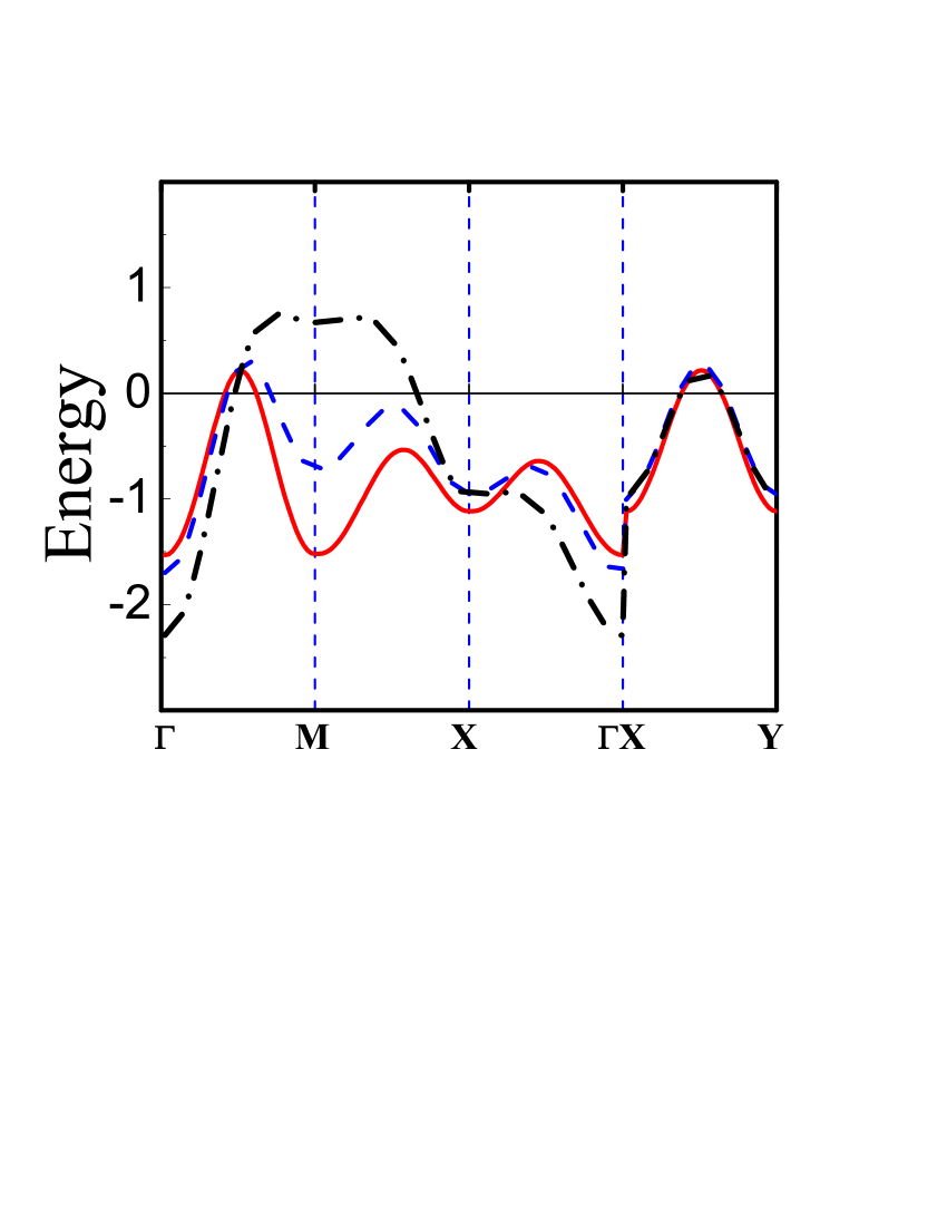
Figure 1: (Color online) Electron dispersion in the MFA ${\varepsilon}_{2}({\bf k})$ along the symmetry directions $\Gamma(0,0)\rightarrow M(\pi,\pi)\rightarrow X(\pi,0)\rightarrow\Gamma(0,0)$ and $X(\pi,0)\rightarrow Y(0,\pi)$ for $\delta=0.05\,$ (red solid line), $0.10$ (blue dashed line), and $0.25$ (black dash-dotted line). Fermi energy for hole doping is at $\omega=0$.

At first we consider results in the MFA for the electronic spectrum (25). The doping dependence of the electron dispersion for the two-hole subband ${\varepsilon}_{2}({\bf k})$ along the symmetry directions in the 2D Brillouin zone (BZ) is shown in Fig. 1. For small doping, $\,\delta=0.05$, the energy at the $M(\pi,\pi)$ and $\Gamma(0,0)$ points are nearly equal as in the AF long-range order state. Only small hole-like FS pockets close to the $(\pm\pi/2,\pm\pi/2)$ points emerge at this doping. With increasing doping, the AF correlation length decreases that results in increasing of the electron energy at the $M(\pi,\pi)$ point and at some critical doping $\delta\sim 0.12$ a large FS appears. At the same time, the renormalized two-hole subband width increases with doping from $\widetilde{W}\approx 2\,t$ at $\,\delta=0.05\,$ to $\widetilde{W}\approx 3\,t$ at $\,\delta=0.25$, which, however, remains less than the “bare” Hubbard bandwidth $W=4t\,(1+\delta)$ where short-range AF correlations are disregarded. Note that in the dynamical mean field theory (DMFT) this narrowing of the subbands due to the short-range AF correlations is missed Georges96 ; Kotliar06 , while they are taken into account partly in the cluster DMFT Haule07 . However, as shown in the DMFT the self-energy contribution strongly renormalizes the electronic spectrum found in the MFA.

To consider the self-energy effects in the electronic spectrum a strong coupling approximation (SCA) should be considered by a self-consistent solution of the system of equations for the normal GF (49) and the self-energy (50). In Ref. Plakida07 a detailed investigation of the normal state electronic spectrum for the conventional Hubbard model in SCA was performed. Therefore, here we present only the results of the electronic spectrum computation for the model (1) which are important for further studies of superconductivity in the model. The spectral functions (55) along the symmetry directions are presented in Figs. 2 and 4 for $\delta=0.10$ and $\delta=0.25$, respectively. The dispersion curves given by the maximum of the spectral function (55) at the same doping are displayed in Figs. 3 and 5.

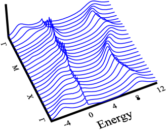
Figure 2: Spectral function in the SCA along the symmetry directions $\Gamma(0,0)\rightarrow M(\pi,\pi)\rightarrow X(\pi,0)\rightarrow\Gamma(0,0)$ for hole concentration $\delta=0.10$.

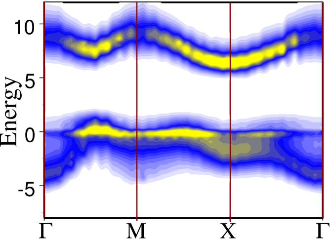
Figure 3: (Color online) Electron dispersion curves in the SCA along the symmetry directions $\Gamma(0,0)\rightarrow M(\pi,\pi)\rightarrow X(\pi,0)\rightarrow\Gamma(0,0)$ for hole concentration $\delta=0.10$.

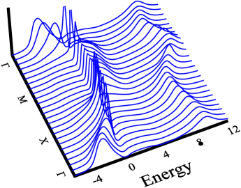
Figure 4: The same as in Fig. 2 for hole concentration $\delta=0.25$.

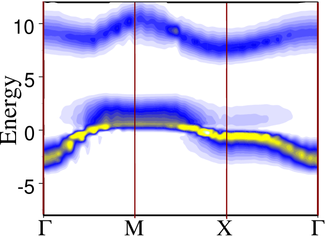
Figure 5: The same as in Fig. 3 for hole concentration $\delta=0.25$.

In comparison with the MFA in Fig. 1, a rather flat energy dispersion is found with QP peaks at the FS. In general, strong increase of the dispersion and intensity of the QP peaks is observed in the overdoped region in comparison with the underdoped region. This is in agreement with our detailed studies of temperature and doping dependence of the self-energy (50) and spectral function (55) in Plakida07 which have proved strong influence of AF spin-correlations on the spectra.

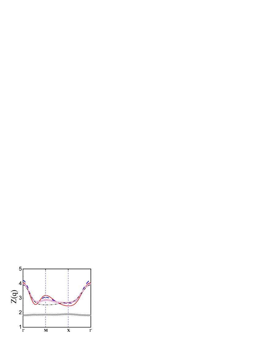
Figure 6: (Color online) Doping dependence of the renormalization parameter $Z({\bf q})$ along the symmetry directions $\Gamma(0,0)\rightarrow M(\pi,\pi)\rightarrow X(\pi,0)\rightarrow\Gamma(0,0)$ at $T\approx 140$ K for $\delta=0.05$ (red solid line), $\delta=0.10$ (blue dashed line), $\delta=0.15$ (pink squares), $\delta=0.25$ (black dash-dotted line), and $\delta=0.35$ (black diamonds).

To estimate the coupling constant $\lambda({\bf q})$ in the two-hole subband, we calculated the renormalization parameter $Z({\bf q})$ (59) at the Fermi energy,

$$Z({\bf q}) = Z({\bf q},\omega=0)=1+\lambda({\bf q})$$ (73)

$$= 1-[\,d\,{\rm Re}\,\Sigma({\bf q},\omega)/{d\omega}]|_{\omega=0}.$$

The doping dependence of $Z({\bf q})$ is shown in Fig. 6. It weakly depends on $\delta$ in the underdoped case for $\delta\lesssim 0.15$ but sharply decreases in the overdoped case for $\delta\gtrsim 0.25$. The temperature dependence of $Z({\bf q})$ presented in Fig. 7 is weak at temperatures lower than the characteristic energy of spin fluctuations $\omega_{s}\sim J$. The EPI gives a small contribution to the coupling constant as follows from the comparison of $Z({\bf q})$ induced by both spin-fluctuations and EPI contributions (red solid line in Fig. 7) with the contribution caused only by spin-fluctuations (blue dashed line).

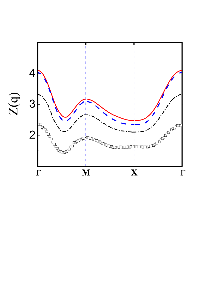
Figure 7: (Color online) Temperature dependence of the renormalization parameter $Z({\bf q})$ for $\delta=0.05$ at $T\approx 140$ K (red solid line), $T\approx 580$ K (black dash-dotted line), and $T\approx 1100$ K (black squares). Blue dashed line shows $Z({\bf q})$ for $\delta=0.05$ caused only by the spin-fluctuation contribution.

The renormalization parameter $X({\bf q})$ (60) at the Fermi energy

$$X({\bf q})=X({\bf q},\omega=0)={\rm Re}{\Sigma}({\bf q},0),$$ (74)

which determines the shift of the dispersion curve is plotted along the symmetry directions in Fig. 8. $X({\bf q})$ decreases with doping in the underdoped region as $Z({\bf q})$, but in the overdoped region reveals an irregular behavior and becomes small at large doping as $Z({\bf q})$. These results demonstrate that at large doping both the electron interaction with spin-fluctuations and the EPI become weak.

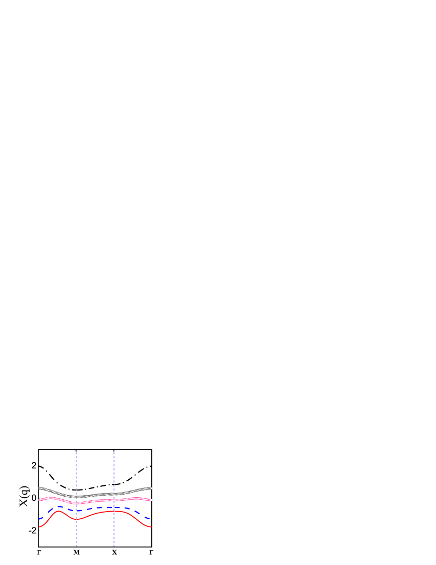
Figure 8: (Color online) Doping dependence of the parameter $X({\bf q})$. Notation are the same as in Fig. 6.

IV.3 Superconducting gap and $\bf T_{c}$

For a comparison of various contributions to the superconducting gap equation (56), as the first step, we consider a weak-coupling approximation (WCA). In the WCA, the interaction (44) is approximated by its value close to the Fermi energy, $\,|\omega,z|\sim 0$. Then integration over $\Omega$ of the dynamical susceptibility in (44) yields

$$\int\limits_{-\infty}^{+\infty}\frac{d\Omega}{\pi}\,\frac{{\rm Im}\,\chi({\bf q},\Omega)}{\omega-z-\Omega}\simeq\int\limits_{-\infty}^{+\infty}\frac{d\Omega}{\pi}\,\frac{{\rm Im}\,\chi({\bf q},\Omega)}{-\Omega}=-\chi({\bf q}),\quad$$ (75)

where $\chi({\bf q})={\rm Re}\,\chi({\bf q},\Omega=0)$ is the static susceptibility. In the WCA the self-energy contribution in the normal-state GF (49) is neglected that results in the BCS-type equation for the gap function at the Fermi energy $\varphi({\bf k})=\sigma\,\varphi_{2,\sigma}({\bf k},\omega=0)$:

$$\varphi({\bf k})=\frac{1}{N}\sum_{\bf q}[1-b({\bf q})]^{2}\frac{\varphi({\bf q})}{2E({\bf q})}\tanh\frac{E({\bf q})}{2T}\big{\{}J({\bf k-q})$$

$$-V({\bf k-q})+\big{[}(1/4)|t({\bf q})|^{2}+|V({\bf k-q})|^{2}\big{]}\chi_{cf}({\bf k-q})$$

$$+|g({\bf k-q})|^{2}\,\chi_{ph}({\bf k-q})\,\theta(\omega_{0}-|\varepsilon_{2}({\bf q})|)$$

$$-|t({\bf q})|^{2}\;\chi_{sf}({\bf k-q})\theta(\omega_{s}-|\varepsilon_{2}({\bf q})|)\big{\}}\,,$$ (76)

where $E({\bf q})=[\varepsilon^{2}_{2}({\bf q})+|\varphi({\bf q})|^{2}]^{1/2}$. Whereas for the exchange interaction and CI there are no retardation effects and the pairing occurs for all electrons in the two-hole subband, the EPI and spin-fluctuation contributions are restricted to the range of energies $\,\pm\omega_{0}$ and $\,\pm\omega_{s}$, respectively, near the FS, as determined by the $\theta$-functions.

To estimate various contributions in the gap equation (76) we consider a model $d$-wave gap function, $\varphi({\bf k})=(\Delta/2)\,\eta({\bf k})$ where $\eta({\bf k})=(\cos k_{x}-\cos k_{y})$. Then the gap equation can be written in the form:

$$1=\frac{1}{N}\sum_{\bf q}[1-b({\bf q})]^{2}\frac{\eta({\bf q})^{2}}{2E_{\bf q}}\tanh\frac{E_{\bf q}}{2T}\big{\{}J-\widehat{V_{c}}$$

$$+\widehat{V}_{cf}+(1/4)\,|t({\bf q})|^{2}\widehat{\chi}_{cf}+\widehat{V}_{ep}\,\theta(\omega_{0}-|\varepsilon_{2}({\bf q})|)$$

$$-|t({\bf q})|^{2}\,\widehat{\chi}_{sf}\theta(\omega_{s}-|\varepsilon_{2}({\bf q})|)\big{\}}.$$ (77)

In this equation only $l=2$ components of the static susceptibility and CI give contributions

$$\widehat{V_{c}} = \frac{1}{N}\sum_{\bf k}V({\bf k})\cos k_{x},$$ (78)

$$\widehat{V}_{cf} = \frac{1}{N}\sum_{\bf k}|V({\bf k})|^{2}\chi_{cf}({\bf k})\,\cos k_{x},$$ (79)

$$\widehat{\chi}_{cf} = \frac{1}{N}\sum_{\bf k}\chi_{cf}({\bf k})\cos k_{x},$$ (80)

$$\widehat{V}_{ep} = \frac{g_{ep}}{N}\sum_{\bf k}S({\bf k})\cos k_{x},$$ (81)

$$\widehat{\chi}_{sf} = \frac{1}{N}\sum_{\bf k}\chi_{sf}({\bf k})\cos k_{x}\,.$$ (82)

Computation yields the following parameters for the n.n. intersite CI (65): $\widehat{V_{c}}=V_{1}=0.44t\approx 0.18$ eV. For the screened CI (66) we have:

$$\widehat{V_{c}}(\kappa) = \frac{u_{c}}{N}\sum_{\bf q}\frac{\cos q_{x}}{q+\kappa},$$ (83)

where $\widehat{V_{c}}(\kappa)=0.12\,t\;(0.28\,t)\approx 0.05\;(0.11)$ eV for $\kappa=1\,(0.2)\,$, respectively (see Table 2). Note, that the projected CI (83) is much smaller than the CI energy $\,V_{c0}(\kappa)=(u_{c}/N)\sum_{\bf q}([1/(q+\kappa)]$. In particular, $\widehat{V_{c}}(\kappa)/V_{c0}(\kappa)=0.15\;(0.24)$ for $\kappa=1,\,(0.2)$, respectively. In the conventional BCS theory the CI is suppressed by retardation effects described by large Bogoliubov-Morel logarithm, $\ln(\mu/\omega_{ph})$. In the Hubbard model there are no retardation effects for the AF exchange interaction but a reduction of the CI contribution is due to the $d$-wave pairing.

To estimate contributions from the charge fluctuations we use the static charge susceptibility (67). Applying this approximation to the screened CI (66) we get the following expression for charge contribution (79):

$$\widehat{V}_{cf}(\kappa) = \frac{u_{c}^{2}}{N}\sum_{\bf k}\,\frac{1}{(k+\kappa)^{2}}\,\chi_{cf}({\bf k})\,\cos k_{x},$$ (84)

where $\,\widehat{V}_{cf}(\kappa)=0.05\;(0.25)\,t\approx 0.02\;(0.1)$ eV for $\kappa=1\,(0.2)$, respectively. This contribution is smaller than the CI repulsion $\widehat{V_{c}}$ (83) and in our approximation the $d$-wave pairing induced by the screened CI in the second order $\widehat{V}_{cf}$ is destroyed by CI repulsion in the first order $\widehat{V_{c}}$ as was pointed out in Ref. Alexandrov11 . The charge fluctuation contribution from the n.n. intersite CI (65) is even smaller, $\;\widehat{V}_{cf}^{nn}\approx 4\cdot 10^{-3}\,t\;$. The contribution from the charge fluctuations (80) calculated for the static susceptibility (67) is also small: $\,\widehat{\chi}_{cf}(\delta)=(1/t)\,0.15\cdot 10^{-2}\;(1.3\cdot 10^{-2})$ for the hole concentrations $\delta=0.05\;(0.10)$, respectively. For the averaged over the BZ vertex $\overline{|t({\bf q})|^{2}}=(1/N)\sum_{\bf q}|t({\bf q})|^{2}\simeq 4\,t^{2}$ this contribution is equal to $\overline{|t({\bf q})|^{2}}\,\widehat{\chi}_{cf}\lesssim 0.02$ eV and can be neglected.

The EPI contribution (81) is given by

$$\widehat{V}_{ep}=\frac{g_{ep}}{N}\sum_{\bf k}\frac{\xi_{ch}^{2}}{1+\xi_{ch}^{2}\,k^{2}}\cos k_{x}\equiv g_{ep}\,S_{d}(\xi_{ch}),$$ (85)

where $S_{d}(\xi_{ch})=0.154\,(0.393)$ for $\xi_{ch}=2\,(10)$, respectively. Thus, even for a strong EPI coupling $g_{ep}=5t=2$ eV we obtain a moderate contribution from the EPI for the $d$-wave pairing: $\widehat{V}_{ep}(\xi_{ch})=0.76\,t\,(1.96\,t)\approx 0.3\,(0.8)$ eV for $\,\xi_{ch}=2\,(10)$, respectively. The EPI contribution to the $s$-wave pairing is given by the $l=0$ component $S_{0}=(1/N)\sum_{\bf q}\,S(q)=0.31\;(0.57)\,$ for $\xi_{ch}=2\;(10)$, respectively. The ratio of the $d$-wave $S_{d}$ and the $s$-wave $S_{s}=S_{0}$ components of the EPI matrix elements is equal to $\,(S_{d}/S_{0})=0.43\;(0.60)$ for $\xi_{ch}=2\;(10)$, respectively. This shows that at small hole concentrations $\delta$ (large charge correlation lengths $\xi_{ch}=1/2\delta$) the EPI for the both components are comparable, while for the overdoped case the $d$-wave component $S_{d}$ becomes considerably smaller than the $s$-wave component in agreement with the results of Ref. Zeyher96 .

The spin-fluctuation contribution $\widehat{\chi}_{sf}$ calculated for the model $\chi_{sf}({\bf q})$ in Eq. (68) for several values of the AF correlation length $\xi$ is given in Table 1. Using the averaged over BZ vertex $\,\overline{|t({\bf q})|^{2}}\simeq 4\,t^{2}\,$ we can estimate an effective spin-fluctuation coupling constant as $\,g_{sf}\simeq-4\,t^{2}\,\widehat{\chi}_{sf}=5.3\,(2.4)t\approx 2\,(1)$ eV for $\delta=0.05\,(0.25)$, respectively. Thus, the spin-fluctuation contribution to the pairing in Eq. (77) appears to be the largest. Note, that $\,g_{sf}\,$ is close to the spin-fluctuation coupling constant $\widetilde{U}\approx 1.6$ eV found in Ref. Dahm09 from ARPES data.

Table 2: CI parameters $\widehat{V}_{c},\,{V}_{c0},\;\widehat{V}_{cf}$, and EPI parameter $\widehat{V_{ep}}$ for several values of the CI screening constant $\kappa=4\delta$ and the charge correlation length $\xi_{cf}=1/2\delta$ for EPI related to hole concentration $\delta$.

$\;\delta\quad$	$\;\kappa\quad$	$\;\xi_{cf}\;$	$\;\widehat{V}_{c}\,/t\quad$	$\;{V}_{c0}\,/t\quad$	$\;\widehat{V}_{cf}\,/t\quad$	$\;\widehat{V_{ep}}\,/t\;$
0.05	0.2	10	0.28	1.18	0.25	1.96
0.10	0.4	5	0.22	1.05	0.26	1.4
0.25	1	2	0.12	0.80	$0.05\;$	0.76

In Table 2 we present the coupling parameters in the equation for $T_{c}$ (77). In the MFA the pairing can be induced by the AF exchange interaction $J=0.4t=0.16$ eV which is comparable with the repulsion caused by the screened CI: $\widehat{V_{c}}=(0.05-0.11)$ eV or even smaller than the n.n. hole CI $V_{1}=0.175$ eV. Therefore, the superconducting pairing in the MFA for the $t$-$J$ model (in particular, the RVB state  Anderson87 ) is strongly suppressed (or even destroyed) by the intersite Coulomb repulsion.

To calculate doping dependence of $T_{c}$ we solve Eq. (77) by taking into account the exchange interaction $J$, the Coulomb repulsion $\widehat{V_{c}}$, and the contributions from the self-energy in the WCA: $\,\widehat{V}_{ep}$, $\widehat{\chi}_{sf}$, and $\,\widehat{V}_{cf}$, neglecting the small contribution $\widehat{\chi}_{cf}$. Results of the calculation is shown in Fig. 9. The highest $T_{c}\approx 0.2\,t$ is found when all the contributions are taken into account. The spin-fluctuation pairing results in superconducting $T^{sf}_{c}\approx 0.04\,t$ much larger than $T^{ep}_{c}\approx 0.01t$ mediated by the EPI. For the ${\bf k}$-independent EPI ($S({\bf k})=1$) as in the Holstein model, the $d$-wave pairing is absent. The doping dependence of $T_{c}$ is qualitatively agree with experiments in cuprates but its value is an order of magnitude higher.

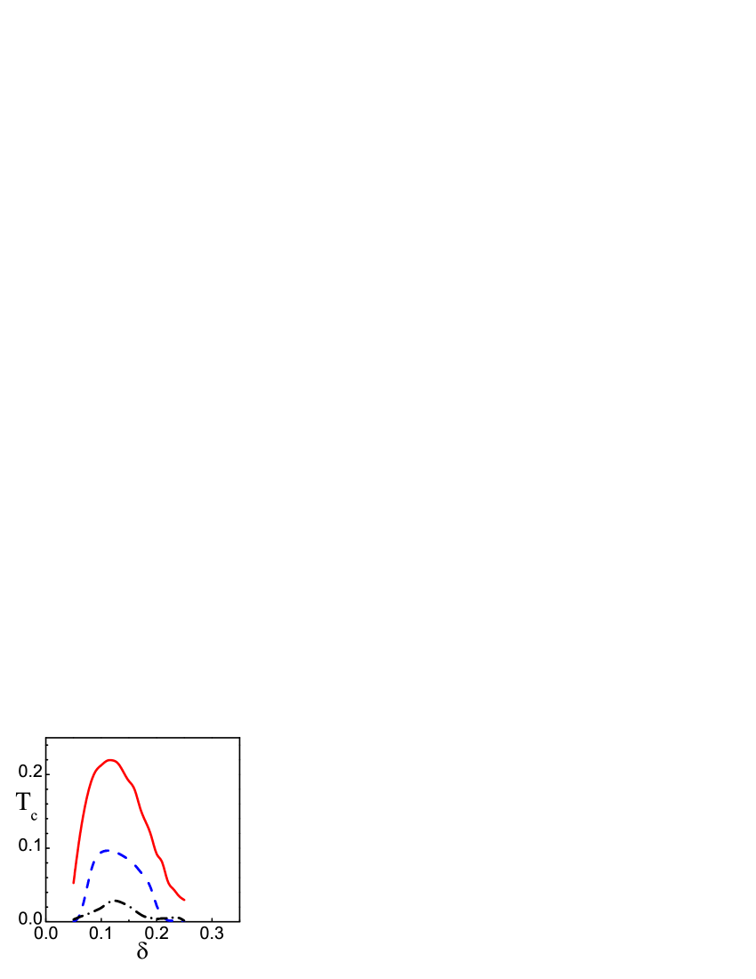
Figure 9: (Color online) $T_{c}(\delta)$ in the WCA induced by all interactions (red solid line) and only by the spin-fluctuation contribution $\widehat{\chi}_{sf}$(blue dashed line) or only by the EPI $\,\widehat{V}_{ep}$ (black dash-dotted line).

The high values for $T_{c}$ found in the WCA are explained by neglecting the reduction of the quasiparticle weight caused by the self-energy effects in the gap equation (III.3). It is convenient to write the gap equation in the form:

$$\varphi({\bf k},\omega_{n})=\frac{T_{c}}{N}\sum_{\bf q}\,\sum_{m}\,\big{\{}J({\bf k-q})-V_{c}({\bf k-q})$$

$$-V_{sf}({\bf q,k-q},\omega_{n}-\omega_{m})+V_{ep}({\bf k-q},\omega_{n}-\omega_{m})\big{\}}$$

$$\times\frac{[1-b({\bf q})]^{2}\,\varphi({\bf q},\omega_{m})}{[\omega_{m}Z({\bf q},\omega_{m})]^{2}+[{\varepsilon}_{2}({\bf q})+X({\bf q},\omega_{m})]^{2}}\,.$$ (86)

For $V_{c}({\bf k-q})$ we take the screened CI (66). Since the charge-fluctuations gives a much weaker contribution than the spin-fluctuation and electron-phonon interactions (see Table 1 and Table 2), we neglect the term $[|V({\bf k-q})|^{2}+|t({\bf q})|^{2}/4]\,\chi_{cf}({\bf k-q},\nu_{n})$ in the interaction function(64). Contributions induced by spin-fluctuations and the EPI are described by the functions

$$V_{sf}({\bf q,k-q},\omega_{\nu})=|t({\bf q})|^{2}\,\chi_{sf}({\bf k-q})F_{sf}(\omega_{\nu}),\quad$$ (87)

$$V_{ep}({\bf k-q},\omega_{\nu})=g_{ep}\,\frac{\omega_{0}^{2}}{\omega^{2}_{0}+\omega_{\nu}^{2}}\,S({\bf k-q}),$$ (88)

where the spectral function for spin fluctuations reads:

$$F_{sf}(\omega_{\nu})=\frac{1}{\pi}\int_{0}^{\infty}\frac{2xdx}{x^{2}+(\omega_{\nu}/\omega_{s})^{2}}\frac{\tanh(x\,\omega_{s}/2T)}{1+x^{2}}\,.$$ (89)

To calculate $T_{c}$ and to find out the energy- and ${\bf k}$-dependence of the gap $\,\varphi({\bf k},\omega)$, Eq. (86) was solved by a direct diagonalization in $(k_{x},k_{y},\,\omega_{n})$-space. Since the largest contribution in Eq. (86) comes from energies close to the FS, we have used the renormalization parameters at the Fermi energy $Z({\bf q})$ (73) and $X({\bf q})$ (74) instead of the energy dependent ones. The results for $T_{c}(\delta)$ is shown in Fig. 10. The highest $T_{c}\sim 0.021t\sim 100$ K is found when all the contributions are taken into account, though pairing induced only by spin-fluctuations also results in high $T^{sf}_{c}\sim 0.014t\sim 65$ K. The $d$-wave pairing induced only by the EPI is rather weak and does not displayed in Fig. 10. The value of $T_{c}$ is reduced by an order of magnitude in comparison with the WCA in Fig. 9 due to a suppression of the QP weight by the factor $[1/Z({\bf q})]^{2}$. The maximum value of $T_{c}$ is found at lower value of doping $\delta_{opt}\approx 0.12$ than in experiments, $\delta^{exp}_{opt}=0.16$.

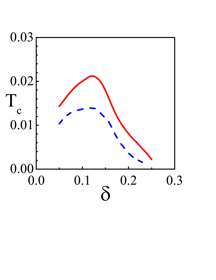
Figure 10: (Color online) $T_{c}(\delta)$ induced by all interactions in Eq. (86) (red solid line) and only by spin-fluctuation contribution $V_{sf}$ (blue dashed line).

The ${\bf k}$-dependence of the gap function $\varphi({\bf k},\omega\simeq 0)\,$ at doping $\delta=0.13$ for $\,(0\leq k_{x},\,k_{y}\leq 2\pi)$ is plotted in Fig. 11. The gap reveals a distinct $d$-wave symmetry with maximum values in the vicinity of the FS. As shown in Fig. 12, its angle dependence on the FS is close to the model $d$-wave dependence $\varphi_{d}(\theta)=\cos 2\theta$.

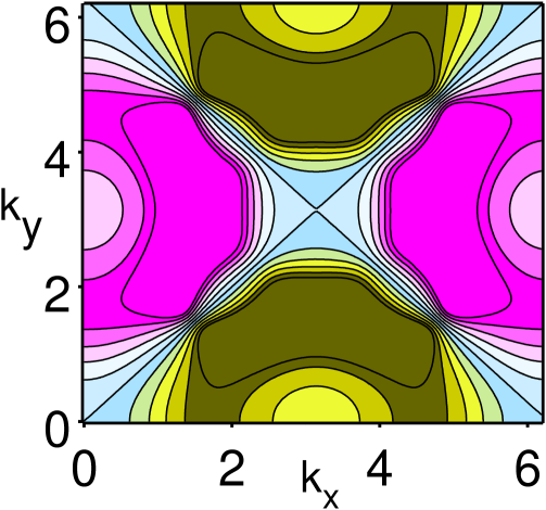
Figure 11: (Color online) 2D plot of the SC gap $\varphi({\bf k},\omega\simeq 0)$.

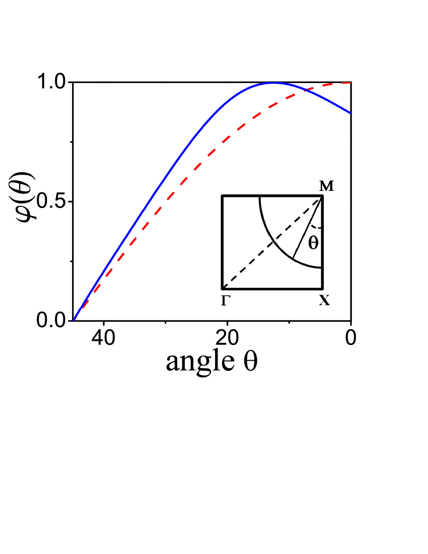
Figure 12: (Color online) Angle dependence of the SC gap $\varphi(\theta)$ on the FS (blue bold line) in comparison with the model $d$-wave dependence $\varphi_{d}(\theta)=\cos 2\theta$ (red dashed lines).

Energy dependence (in units of $\,t\,$) of the gap function $\varphi({\bf k},\omega)$, the real and imaginary parts, is presented in Fig. 13 at ${\bf k}\approx(0,\pi/2)$ and $\delta=0.13$. Since the gap function was obtained as a solution of the linear equation at $T=T_{c}$ the value of the gap is given in arbitrary units. The energy variation of the gap occurs in the region of $\omega\lesssim 0.4t$, of the order of the characteristic spin-fluctuation energy $\omega_{s}=J=0.4t$.

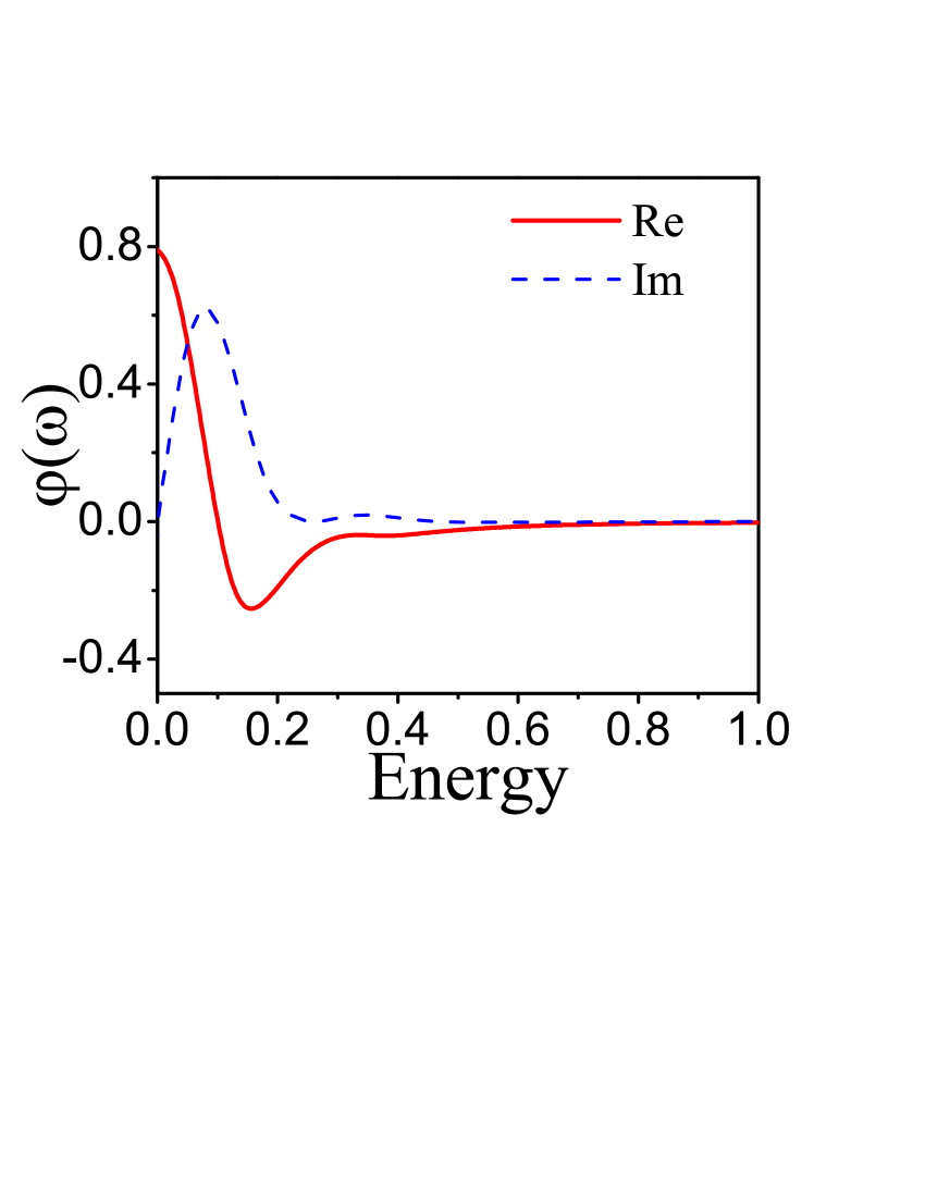
Figure 13: Energy dependence of the real, Re $\varphi({\bf k},\omega)$, and imaginary, Im $\varphi({\bf k},\omega)$, parts of the SC gap in arbitrary units.

Generally, the results obtained in the SCA are in a qualitative agreement with experiments in the cuprate superconductors. They also demonstrate an important role of the self-energy effects in the normal and superconducting states in comparison with the MFA.

IV.4 Comparison with previous theoretical studies

As briefly discussed in Sec. I, various methods have been used in theoretical studies of superconductivity in the Hubbard model. Here we would like to emphasize our results in comparison with previous investigations of the problem.

At first we refer to results obtained in the weak or intermediate correlation limit. In particular, using the two-particle self-consistent non-perturbative approach (see, e.g. Refs. Vilk95 ; Tremblay06 ) and the fluctuation-exchange (FLEX) approximation (see, e.g., Refs. Bickers89 ; Monthoux94a and reviews Moriya00 ; Manske04 ), a system of equations was derived within the Fermi-liquid model to study self-consistently single-electron GFs and the spin and charge dynamical susceptibility. Within the FLEX approximation, the superconducting $d$-wave pairing was found in a narrow range of doping, very close to the AF instability. In our theory superconductivity is mediated by a broad spectrum of AF spin excitations (paramagnons) which results in the doping dependence of $T_{c}$ close to experimentally observed (see Figs. 9, 10).

A general problem of the weak CI in the Hubbard model has been extensively studied within the RG approach (for reviews see Refs. Shankar94 ; Metzner98 ). The RG studies revealed a competition between various type of phases driven by electronic instability, such as the spin-density wave (SDW), charge-density wave (CDW), nematic (Pomeranchuk) phase, stripes, superconducting pairing, etc. (see reviews  Kivelson03 ; Vojta09 and Refs. Furukawa98 ; Honer01 ; Honer07 ; Halb00a ; Halb00b ). For a weak Hubbard interaction $U\sim t$ in a certain range of hopping parameters and doping the $d$-wave superconducting pairing can overcome other instabilities. An important role of the intersite Coulomb repulsion in the Hubbard model was found in Ref. Raghu12 , as mentioned in Sec. I. In our theory we disregarded other instabilities and did not study a general phase diagram since it would demand investigation of a much more complicated system of equations which is beyond the scope of the present paper.

To consider cuprate superconductors, the strong correlation limit should be investigated. In many publications the spectrum of electronic excitations in the normal state in the Hubbard model was extensively studied. Here we refer to numerical simulations for finite clusters (see reviews Dagotto94 ; Bulut02 ; Scalapino07 ), the DMFT (see reviews Georges96 ; Kotliar06 ), the dynamical cluster approximation (DCA) Maier05 ; Maier06 and the cluster DMFT (see, e.g., Refs. Haule07 ; Kancharla08 ). More accurate results have been obtained within the DCA and cluster DMFT methods where short-range AF correlations are partially taken into account. As we have pointed out in Sec. III.1 and Sec. IV.2, in our method short-range AF correlations are properly taken into consideration in the MFA resulting in a large reduction of the effective bandwidth $\,\widetilde{W}$. Consequently, a two-subband state in the Hubbard model is found even in the intermediate correlation limit, $U\sim 4t$. The spectral density computed in SCA, Figs. 2 and 4, are in accord with numerical studies for the Hubbard model (see, e.g., Refs. Maier05 ; Tremblay06 ; Avella07 ).

The most controversial problem is whether the superconductivity can emerge from the repulsion, as discussed in Sec. I. Extensive numerical studies for finite clusters have revealed a tendency to the $d$-wave pairing in the Hubbard model, though a delicate balance between superconductivity and other instabilities (AF, SDW, CDW, etc.) was found (see, e.g., Refs. Bulut02 ; Scalapino07 ; Maier05 ; Maier06 ; Kancharla08 ). In Ref. Macridin09 ), using the DCA with the quantum Monte Carlo method, the superconducting $d$-wave pairing and the isotope effect similar to observed in cuprates were found for the Hubbard-Holstein model. However, in several publications an appearance of the long-range superconducting order has not been confirmed (see, e.g., Ref. Aimi07 ). Therefore, analytical studies are desirable to elucidate this problem.

An accurate analytical method is based on the HO technique where the HO algebra is implemented rigorously. The superconducting pairing induced by the kinematic interaction for the HOs was first proposed by Zaitsev and Ivanov Zaitsev87 who studied the two-particle vertex equation by applying the diagram technique for HOs. The momentum-independent $s$-wave pairing was found in the lowest order diagram approximation equivalent to the MFA. However, this solution violates the HO kinematics and the $t$–$J$ model should be used to obtain the $d$-wave pairing mediated by the AF superexchange interaction (see, e.g., Refs. Plakida89 ; Yushankhai91 ; Plakida99 ; Prelovsek05 ). In this respect we should point out that in many publications superconductivity in the $t$–$J$ model was studied in the MFA (see, e.g., Refs. Plakida89 ; Yushankhai91 ; Valkov02 ; Jedrak10 ). As we have shown in Sec. IV.3, the intersite Coulomb repulsion suppresses or even destroy superconductivity induced by the AF superexchange interaction in the MFA. In particular, in cuprates, a sufficiently strong n.n. hole repulsion $V_{1}=0.1-0.2$ Feiner96 may be detrimental for the RVB state Anderson87 . The same remark refers to the studies of superconductivity in the conventional Hubbard model in the MFA (see, e.g., Refs. Beenen95 ; Avella97 ; Stanescu00 ; Adam07 ). Therefore, consideration of the spin-fluctuation pairing beyond the MFA is essential in description of superconductivity in cuprates as discussed in detail in Sec. IV.3.

In comparison with studies of the intersite Coulomb repulsion in the weak correlation limit in Refs. Alexandrov11 ; Raghu12 , in the strong correlation limit the intersite Coulomb repulsion $V_{ij}$ to some extent is compensated by the nonretarded superexchange interaction $J_{ij}$ (see Eqs. (31), (32)) which is absent in the weak correlation limit. At the same time, even for a sufficiently large component $V_{c0}$ of the CI $V_{ij}$, the contribution to the gap equation is given by a much smaller $d$-wave partial harmonic (83) and therefore is not so detrimental to superconductivity in comparison with the conventional $s$-wave momentum-independent pairing.

Studies of the spin-fluctuation $d$-wave pairing in the presence of the EPI have shown that depending on the symmetry, the EPI could enhance or suppress superconducting pairing (see, e.g., Ref. Plakida94 ; Shneider09 ). In Ref. Lichtenstein95 the $d$-wave pairing induced by both the spin-fluctuations and EPI in the model (71) within the FLEX approximation was considered. It was revealed that a momentum-independent EPI strongly suppresses $T_{c}$, while the EPI with strong forward scattering can enhance $T_{c}$. In our theory the strong spin-fluctuation pairing is induced by the kinematic interaction which is absent in the weak correlation limit as in FLEX approximation, and therefore, the EPI plays only a secondary role in the $d$-wave pairing. A strong EPI in polaronic effects observed in the oxygen isotope effect on the in-plane penetration depth in cuprates Khasanov04 may be irrelevant for the pairing mediated by the $d$-wave partial harmonic of the EPI  Plakida11 as confirmed by a weak isotope effect on $T_{c}$ in the optimally doped cuprates.

V Conclusion

In the paper the theory of superconducting pairing within the extended Hubbard model (1) in the limit of strong electron correlations is presented. Using the Mori-type projection technique we obtained a self-consistent system of equations for normal and anomalous (pair) GFs and for the self-energy calculated in the NCA. The theory is similar to the Migdal-Eliasberg strong-coupling approximation.

We can draw the following conclusions about the mechanism of pairing in the extended Hubbard model. Solution of the gap equation in the weak coupling approximation (76) shows that for the $d$-wave pairing the intersite Coulomb repulsion gives a small contribution determined by $\,l=2\,$ harmonic of the interaction function $V({\bf k-q})$. However, it can be larger than the AF superexchange interaction $\,J({\bf k-q})\,$, and the RVB-type superconducting pairing can be destroyed.

Pairing induced by charge fluctuations $\chi_{ch}({\bf k-q})$ appears to be quite weak (outside the charge-instability region). We have found that the $d$-wave component of the EPI, even for the model of strong forward scattering Zeyher96 and a large fully symmetric $s$-wave component, turned out to be small. The largest contribution to the $d$-wave pairing comes from the electron interaction with spin fluctuations induced by strong kinematic interaction $|t({\bf q})|^{2}$, so that the EPI plays a secondary role in achieving high-$T_{c}$.

It is important to point out that the superconducting pairing induced by the AF superexchange interaction and spin-fluctuation scattering are caused by the kinematic interaction characteristic of systems with strong correlations. These mechanisms of superconducting pairing are absent in the fermionic models (for a discussion, see Ref. Anderson97 ) and are generic for cuprates. The intersite Coulomb repulsion is not strong enough to destroy the $d$-wave pairing mediated by spin fluctuations. Therefore, we believe that the magnetic mechanism of superconducting pairing in the Hubbard model in the limit of strong correlations is a relevant mechanism of high-temperature superconductivity in the copper-oxide materials.

Note added in proof. – When this work was submitted, we became aware of references  Plekhanov03 –Senechal12 which consider the extended Hubbard model with the intersite Coulomb repulsion $V$. The results of the references  Plekhanov03 , Senechal12 show that the on-site repulsion $U$ effectively enhances the $d$-wave pairing which survives for large values of $V$ up to $V\sim U/2\gg J$ (Ref. Senechal12 ). This observation supports our model of spin-fluctuation pairing due to the kinematic interaction which emerges only in the strong correlation limit. As long as the Coulomb repulsion $V$ does not exceed the kinematic interaction of the order of the kinetic energy, $V\lesssim 4\,t\,$, the $d$-wave pairing may survive. The small value of $V=J$ found in Ref. Raghu12a is explained by application of the slave-boson representation in the MFA which ignores the kinematic interaction. We would like to thank A.-M. S. Tremblay for valuable discussion who drew our attention to those papers.

Appendix A Pair correlation function in MFA

Here we calculate the pair correlation function $\langle X_{i}^{02}N_{j}\rangle$ considering an equation of motion for the commutator GF $\,L_{ij}(t-t^{\prime})=\langle\langle X_{i}^{02}(t)\mid N_{j}(t^{\prime})\rangle\rangle|_{i\neq j}\,$. The equation for the GF can be written as Plakida03 :

$$\left(\omega-\varepsilon_{2}\right)L_{ij}(\omega) = \sum_{m\neq i,\sigma^{\prime}}\sigma^{\prime}\,t^{12}_{im}\{\langle\langle X_{i}^{0\bar{\sigma}^{\prime}}X_{m}^{0\sigma^{\prime}}|N_{j}\rangle\rangle_{\omega}$$ (90)

$$- \langle\langle X_{i}^{\sigma^{\prime}2}X_{m}^{\bar{\sigma}^{\prime}2}|N_{j}\rangle\rangle_{\omega}\},$$

where we neglected excitation energy proportional to the intraband hopping in comparison with the interband contribution, $|t^{\alpha\alpha}_{im}|\ll|\varepsilon_{2}|\simeq U\,$. The pair correlation function is determined by the equation:

$$\langle X_{i}^{02}N_{j}\rangle=-\frac{1}{\pi}\int^{+\infty}_{-\infty}\,\frac{d\omega}{1-\exp(-\omega/T)}\,{\rm Im}\,L_{ij}(\omega).$$ (91)

The GF $L_{ij}(\omega)$ has two poles, one at $\omega=\varepsilon_{2}$ and another at the energy of a pair excitation given by the GFs at the right-hand side in Eq. (90) of the singly or the doubly occupied subbands. Let us consider the hole doped case, $n=1+\delta>1$ when the chemical potential crosses the two-hole subband, $\,\mu\sim U\,$ and $\varepsilon_{1}=-\mu\sim-U,\;\varepsilon_{2}=2\varepsilon_{1}+U\sim-U\,$. In this case we can neglect the exponentially small contribution of the order of $\,\exp(-U/T)\ll 1\,$ coming from the pole $\omega=\varepsilon_{2}$. The contribution from the GF of the one-hole subband in (90),

$$-\frac{1}{\pi}{\rm Im}\langle\langle X_{i}^{0\bar{\sigma}}X_{m}^{0\sigma}|N_{j}\rangle\rangle_{\omega}\simeq\delta_{mj}\langle X_{i}^{0\bar{\sigma}}X_{j}^{0\sigma}\rangle\delta(\omega-2\varepsilon_{1}),$$ (92)

also gives an exponentially small contribution of the order of $\,{\exp}(-2U/T)\ll 1\,$. Therefore, we can take into account only the contribution from the GF $\,\langle\langle X_{i}^{\sigma^{\prime}2}X_{m}^{\bar{\sigma}^{\prime}2}|N_{j}\rangle\rangle_{\omega}\,$ where the pair excitation energy $\omega\sim|t^{22}_{im}|$. Using the approximation $\,1/(\omega-\varepsilon_{2})\simeq 1/U\,$ which neglects retardation effects an integration over $\omega$ in Eq. (92) gives the following result,

$$\langle X_{i}^{02}N_{j}\rangle = -\frac{1}{U}\,\sum_{m\neq i,\sigma^{\prime}}\,\sigma^{\prime}\,t^{12}_{im}\langle X_{i}^{\sigma^{\prime}2}X_{m}^{\bar{\sigma}^{\prime}2}N_{j}\rangle$$ (93)

$$\simeq -({4t^{12}_{ij}}/{U})\sigma\,\langle X_{i}^{\sigma 2}\,X_{j}^{\bar{\sigma}2}\rangle.$$

The last formula is obtained in the two-site approximation usually applied for the $t$-$J$ model: $\,m=j$, which gives $X_{j}^{\bar{\sigma}2}N_{j}=2X_{j}^{\bar{\sigma}2}$.

Appendix B Self-energy

The normal and anomalous (pair) components of the self-energy operator (35) are given by the matrices:

$$\hat{M}_{ij\sigma}(\omega)=\langle\!\langle{[\widetilde{X_{i}^{\sigma 2}},H]\choose[\widetilde{X_{i}^{0\bar{\sigma}}},H]}\mid([H,\widetilde{X_{j}^{2\sigma}}]\,[H,\widetilde{X_{j}^{\bar{\sigma}0}}])\rangle\!\rangle^{(pp)}_{\omega},\quad$$ (94)

$$\hat{\Phi}_{ij\sigma}(\omega)=\langle\!\langle{\widetilde{X_{i}^{\sigma 2}},H]\choose[\widetilde{X_{i}^{0\bar{\sigma}}},H]}\mid([H,\widetilde{X_{j}^{\bar{\sigma}2}}][H,\widetilde{X_{j}^{0\sigma}}])\rangle\!\rangle^{(pp)}_{\omega},\quad$$ (95)

where $\,[\widetilde{X_{i}^{\alpha,\beta}},H]\,$ and $\,[H,\widetilde{X_{i}^{\alpha,\beta}}]\,$ are the irreducible parts of the commutators determined by Eq. (17). Using equations of motion for the HOs as given, e.g., by Eq. (7) we obtain multiparticle GFs which are determined by products of bosonic and fermionic operators. Let us consider, in particular, contributions to the two-hole subband self-energy given by the kinematic interaction in Eq. (7). The normal component in Eq. (94) reads,

$$M^{22(k)}_{ij\sigma}(\omega)=\sum_{ll^{\prime}\sigma^{\prime}\sigma^{\prime\prime}}t_{il}t_{jl^{\prime}}\,\langle\!\langle B_{i\sigma\sigma^{\prime}}X_{l}^{\sigma^{\prime}2}|X_{l^{\prime}}^{2\sigma^{\prime\prime}}B_{j\sigma\sigma^{\prime\prime}}^{\dagger}\rangle\!\rangle_{\omega}$$

$$=\sum_{ll^{\prime}\sigma^{\prime}\sigma^{\prime\prime}}t_{il}t_{jl^{\prime}}\,\frac{1}{2\pi}\int_{-\infty}^{\infty}dz\frac{e^{\beta z}+1}{(\omega-z)}\int_{-\infty}^{\infty}\!dte^{izt}$$ (96)

$$\times\;\langle X_{l^{\prime}}^{2\sigma^{\prime\prime}}B_{j\sigma\sigma^{\prime\prime}}^{\dagger}|B_{i\sigma\sigma^{\prime}}(t)X_{l}^{\sigma^{\prime}2}(t)\rangle.$$

For the anomalous component in Eq. (95) we have

$$\Phi^{22(k)}_{ij\sigma}(\omega)=-\sum_{ll^{\prime}\sigma^{\prime}\sigma^{\prime\prime}}t_{il}t_{jl^{\prime}}\,\langle\!\langle B_{i\sigma\sigma^{\prime}}X_{l}^{\sigma^{\prime}2}|X_{l^{\prime}}^{\bar{\sigma}^{\prime\prime}2}B_{j\bar{\sigma}\bar{\sigma}^{\prime\prime}}\rangle\!\rangle_{\omega}$$

$$=-\sum_{ll^{\prime}\sigma^{\prime}\sigma^{\prime\prime}}t_{il}t_{jl^{\prime}}\,\frac{1}{2\pi}\int_{-\infty}^{\infty}dz\frac{e^{\beta z}+1}{\omega-z}\int_{-\infty}^{\infty}\!dte^{izt}$$ (97)

$$\times\;\langle X_{l^{\prime}}^{\bar{\sigma}^{\prime\prime}2}B_{j\bar{\sigma}\bar{\sigma}^{\prime\prime}}|B_{i\sigma\sigma^{\prime}}(t)X_{l}^{\sigma^{\prime}2}(t)\rangle,$$

where the bosonic operator $B_{i\sigma\sigma^{\prime}}=B^{22}_{i\sigma\sigma^{\prime}}$ is defined by Eq. (II.1). Using the spectral representation for the thermodynamic GFs Zubarev60 we introduced in Eqs. (96), (97) the multi-particle time-dependent correlation functions. They are calculated in the mode-coupling approximation as described by Eqs. (40), (41). The time-dependent single-particle fermionic and bosonic correlation functions which appear after the two-time decoupling are calculated self-consistently as e.g.,

$$\langle X_{l^{\prime}}^{2\sigma}X_{l}^{\sigma 2}(t)\rangle = \int_{-\infty}^{\infty}d\omega^{\prime}n(\omega^{\prime})e^{-i\omega^{\prime}t}$$ (98)

$$\times [-(1/\pi)]\,{\rm Im}G^{22}_{ll^{\prime}\sigma}(\omega^{\prime}),$$

$$\langle B_{j\sigma\sigma^{\prime}}^{\dagger}|B_{i\sigma\sigma^{\prime}}(t)\rangle = \int_{-\infty}^{\infty}d\omega^{\prime}N(\omega^{\prime})e^{-i\omega^{\prime}t}$$ (99)

$$\times [-(1/\pi)]\,{\rm Im}\langle\!\langle B_{i\sigma\sigma^{\prime}}|B_{j\sigma\sigma^{\prime}}^{\dagger}\rangle\!\rangle_{\omega^{\prime}}.\quad$$

Here $G^{22}_{ll^{\prime}\sigma}(\omega^{\prime})$ is the GF (36) for the two-hole subband and $\langle\!\langle B_{i\sigma\sigma^{\prime}}|B_{j\sigma\sigma^{\prime}}^{\dagger}\rangle\!\rangle_{\omega^{\prime}}$ is the commutator GF for bosonic excitations. Integration over time $t$ in Eqs. (96) and (97) yields

$$M^{22(k)}_{ij\sigma}(\omega)=\int\!\int_{-\infty}^{\infty}\frac{d\omega_{1}d\omega_{2}}{\pi^{2}}\;\frac{1-n(\omega_{1})+N(\omega_{2})}{\omega-\omega_{1}-\omega_{2}}$$

$$\times\sum_{ll^{\prime}\sigma^{\prime}}t_{il}t_{jl^{\prime}}\,{\rm Im}G^{22}_{ll^{\prime}\sigma^{\prime}}(\omega_{1})\,{\rm Im}\langle\!\langle B_{i\sigma\sigma^{\prime}}|B_{j\sigma\sigma^{\prime}}^{\dagger}\rangle\!\rangle_{\omega_{2}},$$ (100)

$$\Phi^{22(k)}_{ij\sigma}(\omega)=-\int\!\int_{-\infty}^{\infty}\frac{d\omega_{1}d\omega_{2}}{\pi^{2}}\;\frac{1-n(\omega_{1})+N(\omega_{2})}{\omega-\omega_{1}-\omega_{2}}$$

$$\times\sum_{ll^{\prime}\sigma^{\prime}}t_{il}t_{jl^{\prime}}\,{\rm Im}F^{22}_{ll^{\prime}\sigma^{\prime}}(\omega_{1})\,{\rm Im}\langle\!\langle B_{i\sigma\sigma^{\prime}}|B_{j\bar{\sigma}\bar{\sigma}^{\prime}}\rangle\!\rangle_{\omega_{2}}.$$ (101)

Taking into account the definition of the bosonic operator (II.1) the bosonic GFs in these equations can be written as

$$\langle\!\langle B_{i\sigma\sigma^{\prime}}|B_{j\sigma\sigma^{\prime}}^{\dagger}\rangle\!\rangle_{\omega}=(1/4)\langle\!\langle N_{i}|N_{j}\rangle\!\rangle_{\omega}\,\delta_{\sigma^{\prime}\sigma}$$

$$+\langle\!\langle S^{z}_{i}|S^{z}_{j}\rangle\!\rangle_{\omega}\,\delta_{\sigma^{\prime}\sigma}+\langle\!\langle X^{\bar{\sigma}\sigma}_{i}|X^{\sigma\bar{\sigma}}_{j}\rangle\!\rangle_{\omega}\,\delta_{\sigma^{\prime}\bar{\sigma}},$$ (102)

$$\langle\!\langle B_{i\sigma\sigma^{\prime}}|B_{j\bar{\sigma}\bar{\sigma}^{\prime}}\rangle\!\rangle_{\omega}=(1/4)\langle\!\langle N_{i}|N_{j}\rangle\!\rangle_{\omega}\,\delta_{\sigma^{\prime}\sigma}$$

$$-\langle\!\langle S^{z}_{i}|S^{z}_{j}\rangle\!\rangle_{\omega}\,\delta_{\sigma^{\prime}\sigma}+\langle\!\langle X^{\bar{\sigma}\sigma}_{i}|X^{\sigma\bar{\sigma}}_{j}\rangle\!\rangle_{\omega}\,\delta_{\sigma^{\prime}\bar{\sigma}}.$$ (103)

After summation over $\sigma^{\prime}$ in (100) for the bosonic GF (102) and the normal GF in the paramagnetic state, $G^{22}_{ll^{\prime}\sigma}(\omega)=G^{22}_{ll^{\prime}\bar{\sigma}}(\omega)$, the spin-fluctuation contribution can be written in the form: $\langle\!\langle S^{z}_{i}|S^{z}_{j}\rangle\!\rangle_{\omega}+\langle\!\langle X^{\bar{\sigma}\sigma}_{i}|X^{\sigma\bar{\sigma}}_{j}\rangle\!\rangle_{\omega}=\langle\!\langle{\bf S}_{i}|{\bf S}_{j}\rangle\!\rangle_{\omega}$. Similar summation over $\sigma^{\prime}$ in (101) for the bosonic GF (103) and the anomalous GF $F^{22}_{ll^{\prime}\sigma}(\omega)=-F^{22}_{ll^{\prime}\bar{\sigma}}(\omega)$, results in the equation: $\,-\langle\!\langle S^{z}_{i}|S^{z}_{j}\rangle\!\rangle_{\omega}\,F^{22}_{ll^{\prime}\sigma}(\omega)+\langle\!\langle X^{\bar{\sigma}\sigma}_{i}|X^{\sigma\bar{\sigma}}_{j}\rangle\!\rangle_{\omega}\,F^{22}_{ll^{\prime}\bar{\sigma}}(\omega)=-\langle\!\langle{\bf S}_{i}|{\bf S}_{j}\rangle\!\rangle_{\omega}\,F^{22}_{ll^{\prime}\sigma}(\omega)$.

Introducing the $\bf q$-representation for the GFs and the self-energies as defined by Eq. (12) for the self-energies (100) and (101) we obtain the expressions:

$$M^{22(k)}({\bf k},\omega) = \frac{1}{N}\sum_{\bf q}\int\limits_{-\infty}^{+\infty}\!\!{\rm d}z\,K^{(+)}_{(k)}(\omega,z|{\bf q},{\bf k-q})$$ (104)

$$\times [-({1}/{\pi})\,\mbox{Im}\,G^{22}({\bf q},z)],$$

$$\Phi_{\sigma}^{22(k)}({\bf k},\omega) = \frac{1}{N}\sum_{\bf q}\int\limits_{-\infty}^{+\infty}\!\!{\rm d}z\,K^{(-)}_{(k)}(\omega,z|{\bf q},{\bf k-q})$$ (105)

$$\times [-({1}/{\pi})\,\mbox{Im}\,F^{22}_{\sigma}({\bf q},z)],$$

where the contribution from the kinematic interaction is given by the kernel

$$K^{(\pm)}_{(k)}(\omega,z|{\bf q},{\bf k-q})=\frac{|t({\bf q})|^{2}}{\pi}\int\limits_{-\infty}^{+\infty}d\Omega\frac{1+N(\Omega)-n(z)}{\omega-z-\Omega}$$

$$\times\big{\{}{\rm Im}\,\chi_{sf}({\bf k-q},\Omega)\pm(1/4){\rm Im}\,\chi_{cf}({\bf k-q},\Omega)\big{\}}.$$ (106)

Here the spin- and charge-susceptibility are defined by Eqs. (45) and (46). By taking into account contributions from the CI and the EPI in Eq.(7) and using the NCA in calculation of the respective time-dependent correlation functions we obtain the kernel (44) for the integral equations (42) and (43).

References

- (1) J. G. Bednorz and K. A. Müller, Z. Phys. B. 64, 189 (1986).
- (2) Handbook of High-Temperature Superconductivity. Theory and Experiment, edited by J.R. Schrieffer and J.S. Brooks (Springer-Verlag, New York, 2007), Chaps. 13–15.
- (3) N. M. Plakida, High-Temperature Cuprate Superconductors (Springer Series in Solid-State Sciences, Vol. 166, Springer-Verlag, Berlin, 2010), Chap. 7.
- (4) P. W. Anderson, Science 235, 1196 (1987); P. W. Anderson, The theory of superconductivity in the high- cuprates (Princeton University Press, Princeton, 1997).
- (5) D.J. Scalapino, Phys. Reports 250, 329 (1995).
- (6) P. Monthoux and D. Pines, Phys. Rev. B 49, 4261 (1994).
- (7) T. Moriya and K. Ueda, Adv. in Physics 49, 555 (2000); Rep. Prog. Phys. 66, 1299 (2003).
- (8) A. V. Chubukov, D. Pines, and J. Schmalian, in The Physics of Conventional and Unconventional Superconductors, edited by K. H. Bennemann and J. B. Ketterson (Springer-Verlag, Berlin, 2004), Vol. I, p. 495; Ar. Abanov, A.V. Chubukov, and J. Schmalian, Advances in Phys. 52, 119 (2003).
- (9) Ar. Abanov, A.V. Chubukov, and M.R. Norman, Phys. Rev. B 78, 220507(R) (2008).
- (10) A.A. Kordyuk, V.B. Zabolotnyy, D.V. Evtushinsky, D.S. Inosov, T.K. Kim, B. Büchner, and S.V. Borisenko, Eur. Phys. J. 188, 153 (2010).
- (11) T. Dahm, V. Hinkov, S.V. Borisenko, A.A. Kordyuk, V.B. Zabolotnyy, J. Fink, B. Büchner, D.J. Scalapino, W. Hanke, and B. Keimer, Nature Phys. 5, 780 (2009).
- (12) Ph. Bourges, in The Gap Symmetry and Fluctuations in High Temperature Superconductors, edited by J. Bok, G. Deutscher, D. Pavuna and S. A. Wolf (Plenum Press, 1998), p. 349.
- (13) M. Le Tacon, G. Ghiringhelli, J. Chaloupka, M. Moretti Sala, V. Hinkov, M.W. Haverkort, M. Minola, M. Bakr, K. J. Zhou, S. Blanco-Canosa, C. Monney, Y. T. Song, G. L. Sun, C. T. Lin, G. M. De Luca, M. Salluzzo, G. Khaliullin, T. Schmitt, L. Braicovich, and B. Keimer, Nature Phys. 7, 725 (2011).
- (14) A.A. Vladimirov, D. Ihle, and N.M. Plakida, Phys. Rev. B 85, 224536 (2012).
- (15) M. L. Kulić, in Lectures on Physics of Highly Correlated Electronic Systems VIII, edited by A. Avella and F. Mancini, AIP Conf. Proc., Vol. 715 (Melville, New York, 2004), p. 75.
- (16) E.G. Maksimov, M.L. Kulić, and O. V. Dolgov, Adv. in Cond. Mat. Phys., Volume 2010, Article ID 423725 (2010) ( DOI: 10.1155/2010/423725)
- (17) S. Raghu, S. A. Kivelson, and D.J. Scalapino, Phys. Rev. B 81, 224505 (2010).
- (18) J. Hubbard, Proc. Roy. Soc. (London) A, 276, 238 (1963).
- (19) A. S. Alexandrov and V.V. Kabanov, Phys. Rev. Lett. 106, 136403 (2011).
- (20) M. Yu. Kagan, D.V. Efremov, M.S. Marienko, and V.S. Valkov. JETP Lett. 93 725 (2011).
- (21) D. V. Efremov, M. S. Mar enko, M.A. Baranov, and M.Yu. Kagan, J. Exp. Theor. Phys. 90, 861 (2000).
- (22) S. Raghu, E. Berg, A.V. Chubukov, and S. A. Kivelson1 Phys. Rev. B 85, 024516 (2012).
- (23) P. Fulde, Electronic correlations in molecules and solids (Springer Verlag, Berlin 1995).
- (24) Strongly Correlated Systems. Theoretical Methods, edited by A. Avella and F. Mancini (Springer Series in Solid-State Sciences, Vol. 171, Springer Verlag, Berlin, 2012).
- (25) R. Zeyher and M. L. Kulić, Phys. Rev. B 53, 2850 (1996).
- (26) H. Mori, Prog. Theor. Phys. 34, 399 (1965).
- (27) N.M. Plakida and V.S. Oudovenko, JETP 104, 230 (2007).
- (28) J. Hubbard, Proc. Roy. Soc. A (London,) 285, 542 (1965).
- (29) L.F. Feiner, J.H. Jefferson, and R. Raimondi, Phys. Rev. B 53, 8751 (1996).
- (30) V.J. Emery, Phys. Rev. Lett. 58, 2794 (1987); C.M. Varma, S. Schmitt-Rink, and E. Abrahams, Solid State Commun. 62, 681 (1987).
- (31) F.C. Zhang and T.M. Rice, Phys. Rev. B 37, 3759 (1988).
- (32) D.N. Zubarev, Usp. Fiz. Nauk 71, 71 (1960); ( Sov. Phys. Usp. 3, 320 (1960)); Nonequilibrium Statical Thermodynamics (Consultant Bureau, New-York, 1974).
- (33) Gh. Adam and S. Adam, J. Phys. A: Math. Theor. 40, 11205 (2007).
- (34) N.M. Plakida, L. Anton, S. Adam, and Gh. Adam, Zh. Exp.Theor. Fyz. 124, 367 (2003), (JETP 97, 331 (2003)).
- (35) N.M. Plakida, Physica C 282–287, 1737 (1997).
- (36) A.B. Migdal, Zh. Eksp. Teor. Fiz. 34, 1438 (1956), (Soviet Phys. JETP 7, 996 (1958)).
- (37) G.M. Eliashberg, Zh. Eksp. Teor. Fiz. 38, 966 (1960); ibid 39, 1437 (1960) (Soviet Phys. JETP 11, 696 (1960); ibid 12, 1000 (1960)).
- (38) Z. Liu and E. Manousakis, Phys. Rev. B 45, 2425 (1992).
- (39) P. Monthoux, Phys. Rev. B 55, 15261 (1997).
- (40) F. Becca, M. Tarquini, M. Grilli, and C. Di Castro, Phys. Rev. B, 54, 12 443 (1996).
- (41) C. Castellani, C. Di Castro, and M. Grilli, J. of Phys. and Chem. of Sol. 59, 1694 (1998).
- (42) T. Ekino, A.M. Gabovich, Mai Suan Li, M. Pȩkała, H. Szymczak, and A.I. Voitenko, J. Phys.: Condens. Matter 23 385701 (2011).
- (43) J. Jaklič and P. Prelovśek, Phys. Rev. Lett. 74, 3411 (1995); ibid. 75, 1340 (1995).
- (44) A.A. Vladimirov, D. Ihle, and N. M. Plakida, Phys. Rev. B 80, 104425 (2009).
- (45) A.I. Lichtenstein. and M.L. Kulić, Physica C 245, 186 (1995).
- (46) A. Georges, G. Kotliar, W. Krauth, and M. Rozenberg, Rev. Mod. Phys. 68, 13 (1996).
- (47) G. Kotliar, S. Y. Savrasov, K. Haule, V.S. Oudovenko, O. Parcollet, and C.A. Marianetti, Rev. Mod. Phys. 78, 865 (2006).
- (48) K. Haule and G. Kotliar, Phys. Rev. B 76, 104509 (2007).
- (49) Y. Vilk and A.-M. Tremblay, J. Phys. Chem. Solids (UK) 56, 1769 (1995); Y. Vilk and A.-M. Tremblay, J. Phys I (France) 7, 1309 (1997); Y. Vilk, L. Chen, and A.-M. Tremblay, Phys. Rev. B 49, 13267 (1994).
- (50) A-M.S. Tremblay, B. Kyung and D. Sénéchal, Fiz. Nizk. Temp. (Low Temp. Phys., Ukraine) 32, 561 (2006); B. Davoudi and A.-M.S. Tremblay, Phys. Rev. B 76, 085115 (2007).
- (51) N.E. Bickers, D.J. Scalapino, and S.R. White, Phys. Rev. Lett. 62, 961 (1989).
- (52) P. Monthoux and D.J. Scalapino, Phys. Rev. Lett. 72, 1874 (1994).
- (53) D. Manske, I. Eremin, and K.H. Bennemann, in The Physics of Conventional and Unconvencional Superconductors, edited by K.H. Bennemann and J.B. Ketterson (Springer-Verlag, Berlin, 2004), Vol. II, p. 731.
- (54) R. Shankar, Rev. Mod. Phys. 66, 129 (1994).
- (55) W. Metzner, C. Castellani, and C. Di Castro, Adv. Phys. 47, 317 (1998).
- (56) S.A. Kivelson, E. Fradkin, V. Oganesyan, I.P. Bindloss, J.M. Tranquada, A. Kapitulnik, and C. Howald, Rev. Mod. Phys. 75, 1201 (2003).
- (57) M. Vojta, Adv. Phys., 58, 699 (2009).
- (58) N. Furukawa, T.M. Rice, and M. Salmhofer, Phys. Rev. Lett. 81, 3195 (1998).
- (59) C. Honerkamp, M. Salmhofer, N. Furukawa, and T. M. Rice, Phys. Rev. B 63, 035109 (2001).
- (60) C. Honerkamp, H. C. Fu, and D.-H. Lee, Phys. Rev. B 75, 014503 (2007).
- (61) C. J. Halboth and W. Metzner, Phys. Rev. B 61, 7364 (2000).
- (62) C. J. Halboth and W. Metzner, Phys. Rev. Lett. 85, 5162 (2000)
- (63) E. Dagotto, Rev. Mod. Phys. 66, 763 (1994).
- (64) N. Bulut, Advances in Physics 51, 1587 (2002).
- (65) D.J. Scalapino, in Handbook of High-Temperature Superconductivity. Theory and Experiment, edited by J.R. Schrieffer and J.S. Brooks (Springer-Verlag, New York, 2007), pp. 495–526.
- (66) Th. Maier, M. Jarrel, Th. Pruschke, and M.H. Hettler, Rev. Mod. Phys. 77, 1027 (2005).
- (67) Th.A. Maier, M. Jarrell, and D.J. Scalapino, Phys. Rev. Lett. 96, 047005 (2006); ibid, Phys. Rev. B 74, 094513 (2006).
- (68) S. S. Kancharla, B. Kyung, D. Sénéchal, M. Civelli, M. Capone, G. Kotliar, and A.-M. S. Tremblay, Phys. Rev. B 77, 184516 (2008).
- (69) A. Avella and F. Mancini, Phys. Rev. B 75, 134518 (2007); A. Avella and F. Mancini, J. Phys.: Condens. Matter 19, 255209 (2007).
- (70) A. Macridin and M. Jarrell, Phys. Rev. B 79, 104517 (2009).
- (71) T. Aimi and M. Imada, J. Phys. Soc. Jpn. 76, 13708 (2007).
- (72) R.O. Zaitsev, and V.A. Ivanov, Soviet Phys. Solid State 29, 2554 (1987), Ibid. 29, 3111 (1987), Int. J. Mod. Phys. B 5, 153 (1988).
- (73) N.M. Plakida, V.Yu. Yushankhai, and I.V. Stasyuk, Physica C 160, 80 (1989).
- (74) V.Yu. Yushankhai, N.M. Plakida, and P. Kalinay, Physica C 174, 401 (1991).
- (75) N.M. Plakida and V.S. Oudovenko, Phys. Rev. B 59, 11949 (1999).
- (76) P. Prelovšek and A. Ramšak, Phys. Rev. B 72, 012510 (2005).
- (77) V.V. Val’kov, T.A. Val’kova, D.M. Dzebisashvili, and S.G. Ovchinnikov, JETP Letters 75, 378 (2002).
- (78) J. Jȩdrak and J. Spałek, Phys. Rev. B 81, 073108 (2010), ibid., 83, 104512 (2011).
- (79) J. Beenen and D.M. Edwards, Phys. Rev. B, 52, 13636 (1995).
- (80) A. Avella, F. Mancini, D. Villani, and H. Matsumoto, Physica C, 282–287, 1757 (1997); T. Di Matteo, F. Mancini, H. Matsumoto, and V.S. Oudovenko, Physica B, 230–232, 915 (1997).
- (81) T.D. Stanescu, I. Martin, and Ph. Phillips, Phys. Rev. B 62, 4300 (2000).
- (82) N.M. Plakida and R. Hayn, Z. Physik B 93, 313 (1994).
- (83) E.I. Shneider and S.G. Ovchinnikov, Zh. Eksp. Teor. Fiz. 136, 1177 (2009).
- (84) R. Khasanov, A. Shengelaya, E. Morenzoni, K. Conder, I.M. Savic̀, and H. Keller, J. Phys.: Condens. Matter 16, S4439 (2004).
- (85) N.M. Plakida, Physica Scripta 83, 038303 (2011).
- (86) P.W. Anderson, Adv. in Physics, 46, 3 (1997).
- (87) E. Plekhanov, S. Sorella, and M. Fabrizio, Phys. Rev. Lett. 90, 187004 (2003)
- (88) S. Raghu, R. Thomale, and T. H. Geballe, Phys. Rev. B 86, 094506 (2012)
- (89) D. Sénéchal, A. Day, V. Bouliane, and A.-M. S. Tremblay, arXiv:1212.4503 (unpublished)