On the heat flux and entropy produced by thermal fluctuations
Abstract
We report an experimental and theoretical analysis of the energy exchanged between two conductors kept at different temperature and coupled by the electric thermal noise. Experimentally we determine, as functions of the temperature difference, the heat flux, the out-of- equilibrium variance and a conservation law for the fluctuating entropy, which we justify theoretically. The system is ruled by the same equations as two Brownian particles kept at different temperatures and coupled by an elastic force. Our results set strong constrains on the energy exchanged between coupled nano-systems held at different temperatures.
pacs:
05.40.-a, 05.70.-a, 05.70.LnThe fluctuations of thermodynamics variables play an important role in understanding the out-of-equilibrium dynamics of small systems sek10 ; Seifert_2012 , such as Brownian particles bli06 ; Jop ; Ruben ; Evans02 ; seifbech2012 , molecular motors kumiko and other small devices Ciliberto . The statistical properties of work, heat and entropy, have been analyzed, within the context of the fluctuation theorem gallavotti and stochastic thermodynamics sek10 ; Seifert_2012 , in several experiments on systems in contact with a single heat bath and driven out-of-equilibrium by external forces or fields bli06 ; Jop ; Ruben ; Evans02 ; kumiko ; Ciliberto ; seifbech2012 . In contrast, the important case in which the system is driven out-of-equilibrium by a temperature difference and energy exchange is produced only by the thermal noise has been analyzed only theoretically on model systems Deridda ; Jarz2004 ; VandenBroeck ; Villamania ; Visco ; Dhar2007 ; Gas2009 ; evans_temp ; Hanggi2011 but never in an experiment because of the intrinsic difficulties of dealing with large temperature differences in small systems.
We report here an experimental and theoretical analysis of the statistical properties of the energy exchanged between two conductors kept at different temperature and coupled by the electric thermal noise, as depicted in fig. 1a. This system is inspired by the proof developed by Nyquist Nyquist in order to give a theoretical explanation of the measurements of Johnson Johnson on the thermal noise voltage in conductors. In his proof, assuming thermal equilibrium between the two conductors, he deduces the Nyquist noise spectral density. At that time, well before Fluctuation Dissipation Theorem (FDT), this was the second example, after the Einstein relation for Brownian motion, relating the dissipation of a system to the amplitude of the thermal noise. In this letter we analyze the consequences of removing the Nyquist’s equilibrium conditions and we study the statistical properties of the energy exchanged between the two conductors kept at different temperature. This system is probably among the simplest examples where recent ideas of stochastic thermodynamics can be tested but in spite of its simplicity the explanation of the observations is far from trivial. We measure experimentally the heat flowing between the two heath baths, and show that the fluctuating entropy exhibits a conservation law. This system is very general because is ruled by the same equations of two Brownian particles kept at different temperatures and coupled by an elastic force VandenBroeck ; Villamania . Thus it gives more insight into the properties of the heat flux produced by mechanical coupling, in the famous Feymann ratchet Feymann ; Smoluchowski ; Abb2000 widely studied theoretically VandenBroeck but never in an experiment.


Therefore our results have implications well beyond the simple system we consider here.
Such a system is sketched in fig.1a). It is constituted by two resistances and , which are kept at different temperature and respectively. These temperatures are controlled by thermal baths and is kept fixed at whereas can be set at a value between and using liquid nitrogen vapor as a circulating coolant. In the figure, the two resistances have been drawn with their associated thermal noise generators and , whose power spectral densities are given by the Nyquist formula , with (see eqs.3,4 and ref.Supplementary ). The coupling capacitance controls the electrical power exchanged between the resistances and as a consequence the energy exchanged between the two baths. No other coupling exists between the two resistances which are inside two separated screened boxes. The quantities and are the capacitances of the circuits and the cables. Two extremely low noise amplifiers and RSI measure the voltage and across the resistances and respectively. All the relevant quantities considered in this paper can be derived by the measurements of and , as discussed below. In the following we will take and , if not differently stated. When the system is in equilibrium and exhibits no net energy flux between the two reservoirs. This is indeed the condition imposed by Nyquist to prove his formula, and we use it to check all the values of the circuit parameters. Applying the Fluctuation-Dissipation-Theorem (FDT) to the circuit, one finds the Nyquist’s expression for the variance of and at equilibrium, which reads with , if and if . For example one can check that at K, using the above mentioned values of the capacitances and resistances, the predicted equilibrium standard deviations of and are and respectively. These are indeed the measured values with an accuracy better than , see ref. Supplementary for further details on the system calibration.
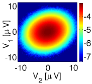
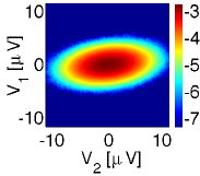
The important quantity to consider here is the joint probability , which is plotted in fig. 2a) at and at fig. 2b) at . The fact that the axis of the ellipses defining the contours lines of are inclined with respect to the and axis indicates that there is a certain correlation between and . This correlation, produced by the electric coupling, plays a major role in determining the mean heat flux between the two reservoirs, as we discuss below. The interesting new features occur of course when . The questions that we address for such a system are: What are the heat flux and the entropy production rate ? How the variance of an are modified because of the heat flux ? What is the role of correlation between and ? We will see that these questions are quite relevant and have no obvious answers because of the statistical nature of the energy transfer.
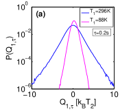
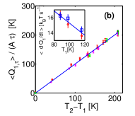
We consider the electric power dissipated in the resistance with which reads where is the current flowing in the resistance . The integral of the power over a time is the total energy , dissipated by the resistance in this time interval, i.e. . All the voltages and currents can be measured: indeed we have where is the current flowing in the capacitance , and is the current flowing in . Thus rearranging the terms one finds that where , and is the potential energy change of the circuit in the time . Notice that are the terms responsible for the energy exchange since they couple the fluctuations of the two circuits. The quantities and can be identified as the work performed by the circuit 2 on 1 and vice-versa Sekimoto ; VanZonCil ; Garnier , respectively. Thus, the quantity () can be interpreted as the heat flowing from the reservoir 2 to the reservoir 1 (from 1 to 2), in the time interval , as an effect of the temperature difference. As the two variables are fluctuating voltages all the other quantities also fluctuate. In fig. 3a) we show the probability density function , at various temperatures: we see that is a strongly fluctuating quantity, whose has long exponential tails.
Notice that although for the mean value of is positive, instantaneous negative fluctuations can occur, i.e., sometimes the heat flux is reversed. The mean values of the dissipated heats are expected to be linear functions of the temperature difference , i.e. , where is a parameter dependent quantity, that can be obtained explicitly from eqs. 3 and 4 below. This relation is confirmed by our experimental results, as shown in fig. 3b. Furthermore, the mean values of the dissipated heat satisfy the equality , corresponding to an energy conservation principle: the power extracted from the bath 2 is dissipated into the bath 1 because of the electric coupling. This mean flow produces a change of the variances of with respect to the equilibrium value , that is the equilibrium value measured when the two baths are at the same temperature . Specifically we find which is an extension to two temperatures of the Harada-Sasa relation harada (see also ref.Supplementary for a theoretical proof of this experimental result). This result is shown in the inset of fig. 3b) where the values of directly estimated from the experimental data (using the steady state ) are compared with those obtained from the difference of the variances of measured in equilibrium and out-of-equilibrium. The values are comparable within error bars and show that the out-of-equilibrium variances are modified only by the heat flux.
It is now important to analyze the entropy produced by the total system, circuit plus heat reservoirs. We consider first the entropy due to the heat exchanged with the reservoirs, which reads . This entropy is a fluctuating quantity as both and fluctuate, and its average in a time is . However the reservoir entropy is not the only component of the total entropy production: one has to take into account the entropy variation of the system, due to its dynamical evolution. Indeed, the state variables also fluctuate as an effect of the thermal noise, and thus, if one measures their values at regular time interval, one obtains a “trajectory” in the phase space . Thus, following Seifert Seifert , who developed this concept for a single heat bath, one can introduce a trajectory entropy for the evolving system , which extends to non-equilibrium systems the standard Gibbs entropy concept. Therefore, when evaluating the total entropy production, one has to take into account the contribution over the time interval of
| (1) |
It is worth noting that the system we consider is in a non-equilibrium steady state, with a constant external driving . Therefore the probability distribution (as shown in fig. 2b)) does not depend explicitly on the time, and is non vanishing whenever the final point of the trajectory is different from the initial one: . Thus the total entropy change reads , where we omit the explicit dependence on , as the system is in a steady-state as discussed above. This entropy has several interesting features. The first one is that , and as a consequence which grows with increasing . The second and most interesting result is that independently of and of , the following equality always holds:
| (2) |
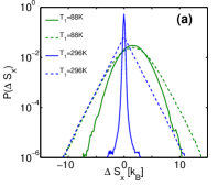
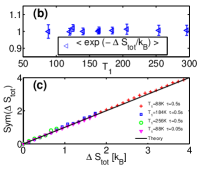
for which we find both experimental evidence, as discussed in the following, and provide a theoretical proof in ref. Supplementary . Equation (2) represents an extension to two temperature sources of the result obtained for a system in a single heat bath driven out-of-equilibrium by a time dependent mechanical force Seifert ; Evans02 and our results provide the first experimental verification of the expression in a system driven by a temperature difference. Eq. (2) implies that , as prescribed by the second law. From symmetry considerations, it follows immediately that, at equilibrium (), the probability distribution of is symmetric: . Thus Eq. (2) implies that the probability density function of is a Dirac function when , i.e. the quantity is rigorously zero in equilibrium, both in average and fluctuations, and so its mean value and variance provide a measure of the entropy production. The measured probabilities and are shown in fig. 4a). We see that and are quite different and that the latter is close to a Gaussian and reduces to a Dirac function in equilibrium, i.e. (notice that, in fig.4a, the small broadening of the equilibrium is just due to unavoidable experimental noise and discretization of the experimental probability density functions). The experimental measurements satisfy eq. (2) as it is shown in fig. 4b). It is worth to note that eq. (2) implies that should satisfy a fluctuation theorem of the form , as discussed extensively in reference EVDB10 ; Seifert_2012 . We clearly see in fig.4c) that this relation holds for different values of the temperature gradient. Thus this experiment clearly establishes a relationship between the mean and the variance of the entropy production rate in a system driven out-of-equilibrium by the temperature difference between two thermal baths coupled by electrical noise. Because of the formal analogy with Brownian motion the results also apply to mechanical coupling as discussed in the following.
We will now give a theoretical interpretation of the experimental observations. This will allow us to show the analogy of our system with two interacting Brownian particles coupled to two different temperatures, see fig. 1-b). Let () be the charges that have flowed through the resistances , so the instantaneous current flowing through them is . A circuit analysis shows that the equations for the charges are:
| (3) | |||||
| (4) |
where is the usual white noise: . The relationships between the measured voltages and the charges are:
| (5) | |||||
| (6) |
Eqs. 3 and 4 are the same of those for the two coupled Brownian particles sketched in fig.1b) by considering the displacement of the particle , its velocity, the stiffness of the spring , the coupling spring and the viscosity. With this analogy we see that our definition of the heat flow corresponds exactly to the work performed by the viscous forces and by the bath on the particle , and it is consistent with the stochastic thermodynamics definition Sekimoto ; VanZonCil ; Seifert_2012 ; alb1 ; alb2 . Thus our theoretical analysis and the experimental results apply to both interacting mechanical and electrical systems coupled to baths at different temperatures. Starting from eqs. (3)-(4), we can prove (see ref. Supplementary ) that eq.2 is an exact result and that the average dissipated heat rate is
| (7) |
with and is the parameter used to rescale the data in fig. 3b).
To conclude we have studied experimentally the statistical properties of the energy exchanged between two heat baths at different temperature which are coupled by electric thermal noise. We have measured the heat flux, the entropy production rate and we have shown the existence of a conservation law for entropy which imposes the existence of a fluctuation theorem which is not asymptotic in time. Our results, which are theoretically proved, are very general since the electric system considered here is ruled by the same equations as for two Brownian particles, held at different temperatures and mechanically coupled. Therefore these results set precise constraints on the energy exchanged between coupled nano and micro-systems held at different temperatures. We finally mention that for the quantity an asymptotic fluctuation theorem can be proved both experimentally and theoretically, and this will be the subject of a paper in preparation.
References
- (1) U. Seifert Rep. Progr. Phys. 75, 126001, (2012).
- (2) Sekimoto, K. Stochastic Energetics. (Springer, 2010).
- (3) Blickle V., Speck T., Helden L., Seifert U., and Bechinger C. Phys. Rev. Lett. 96, 070603 (2006).
- (4) Jop, P., Petrosyan A. and Ciliberto S. EPL 81, 50005 (2008).
- (5) Gomez-Solano, J. R., Petrosyan, A., Ciliberto, S. Chetrite, R. and Gawedzki K. Phys. Rev. Lett 103, 040601 (2009).
- (6) G. M. Wang, E. M. Sevick, E. Mittag, D. J. Searles, and D. J. Evans, Phys. Rev. Lett., 89: 050601 (2002).
- (7) J. Mehl, B. Lander, C. Bechinger, B. Blicke and U. Seifert, Phys. Rev. Lett. 108, 220601 (2012).
- (8) K. Hayashi, H. Ueno, R. Iino, H. Noji, Phys. Rev. Lett. 104, 218103 (2010)
- (9) S Ciliberto, S Joubaud and A Petrosyan J. Stat. Mech., P12003 (2010).
- (10) D. J. Evans et al., Phys. Rev. Lett. 71, 2401 (1993); G. Gallavotti, E. G. D. Cohen, J. Stat. Phys. 80, 931 (1995).
- (11) T. Bodinau, B. Deridda, Phy.Rev. Lett 92, 180601 (2004).
- (12) C. Jarzynski and D. K. Wójcik Phys. Rev. Lett. 92, 230602 (2004).
- (13) C. Van den Broeck, R. Kawai and P. Meurs, Phys. Rev. Lett 93, 090601 (2004).
- (14) P Visco, J. Stat. Mech., page P06006, (2006).
- (15) K. Saito and A. Dhar Phys. Rev. Lett. 99, 180601 (2007).
- (16) D. Andrieux, P. Gaspard, T. Monnai, S. Tasaki, New J. Phys. 11, 043014 (2009).
- (17) Evans D. , Searles D. J. Williams S. R., J. Chem. Phys. 132, 024501 2010.
- (18) M. Campisi, P. Talkner, P. Hanggi, Rev. Mod. Phys. 83, 771 (2011)
- (19) A. Crisanti, A. Puglisi, and D. Villamaina, Phys. Rev. E 85, 061127 (2012)
- (20) H. Nyquist, Phys. Rev. 32, 110 (1928)
- (21) J. Johnson, Phys. Rev. 32, 97 (1928)
- (22) R. P. Feynman, R. B. Leighton, and M. Sands, The Feynman Lectures on Physics I (Addison-Wesley, Reading, MA, 1963), Chap. 46.
- (23) M. v. Smoluchowski, Phys. Z. 13, 1069 (1912).
- (24) D. Abbott, B. R. Davis, and J. M. R. Parrondo, AIP Conf. Proc. 511, 213 (2000).
- (25) Sekimoto K, Prog. Theor. Phys. Suppl. 130, 17, (1998)
- (26) Supplementary Material.
- (27) N. Garnier, S. Ciliberto, Phys. Rev. E, 71, 060101(R) (2005)
- (28) U. Seifert, Phys. Rev. Lett., 95: 040602 (2005).
- (29) M. Esposito, C. Van den Broeck, Phys. Rev. Lett., 104, 090601 (2010).
- (30) R. van Zon, S. Ciliberto, E. G. D. Cohen,Phys. Rev. Lett. 92: 130601 (2004).
- (31) A. Imparato, L. Peliti, G. Pesce, G. Rusciano, A. Sasso, Phys. Rev. E, 76: 050101R (2007).
- (32) H. C. Fogedby, A. Imparato, J. Stat. Mech. P04005 (2012).
- (33) G. Cannatá, G. Scandurra, C. Ciofin,Rev. Scie. Instrum. 80,114702 (2009).
- (34) Harada T. Sasa S.-I.,Phys. Rev. Lett.,95,130602(2005).
See pages 1,, 2, 3, 4, 5, 6 of supp_mat_4.pdf