Inferring the Rate-Length Law of Protein Folding

Abstract

We investigate the rate-length scaling law of protein folding, a key undetermined scaling law in the analytical theory of protein folding. We demonstrate that chain length is a dominant factor determining folding times, and that the unambiguous determination of the way chain length correlates with folding times could provide key mechanistic insight into the folding process. Four specific proposed laws (power law, exponential, and two stretched exponentials) are tested against one another, and it is found that the power law best explains the data. At the same time, the fit power law results in rates that are very fast, nearly unreasonably so in a biological context. We show that any of the proposed forms are viable, conclude that more data is necessary to unequivocally infer the rate-length law, and that such data could be obtained through a small number of protein folding experiments on large protein domains.

I Introduction

A deep understanding of protein folding must involve a description of the general mechanisms involved. It is reasonable to suspect this will consist of a simple model, based on microscopic physics, expressed in a simple mathematical language. Such a model would show how biological sequences are able to employ physics to spontaneously self-assemble into intricate molecular machines.

Simple models of this sort often start by postulating a mechanism of folding, and then derive the consequences of that mechanism Lane and Pande (2012); Gutin et al. (1996); Cieplak and Hoang (2003); Cieplak et al. (1999); Zwanzig et al. (1992); Zwanzig (1995); Thirumalai (1995); Li et al. (2002); Naganathan and Muñoz (2005); Koga and Takada (2001); Finkelstein et al. (2007); Wolynes (1997). This suggests it might be possible to infer the general mechanisms of protein folding by verifying the specific predictions of these models. For a simple model of protein folding, however, there is a limited set of general experimental trends that can be readily predicted. One such experimental trend is the law governing how folding times scale with chain length. This is perhaps the simplest comparison of theory and experiment possible, but has not yet been unambiguously inferred despite nearly two decades of active research Thirumalai (1995); Gutin et al. (1996).

The rate-length law is also an interesting result in and of itself. Such a law can be viewed as a statement of the computational complexity of protein folding – given a problem of size $N$ (residues), how does one expect the time-to-solution (folding) to scale? Levinthal pointed out that an exhaustive search would result in exponential scaling, and suggested that this would result in unreasonably large folding times Levinthal (1969). Thus, in many ways, a resolution to Levinthal’s paradox is likely to be phrased directly as a rate scaling law, either non-exponential (polynomial) or exponential with an explicitly small exponential factor.

A number of issues complicate inferring such a law from experiment, most importantly the fact that available kinetic data on protein folding spans a very limited range of chain lengths - about 30 to 300 residues Bogatyreva et al. (2009). The statistical power of the data is inherently limited by the fact that protein domain sizes barely span a single order of magnitude, and that most studies of folding have focused on small, well-behaved model systems.

Further complicating the inference of the rate-length scaling law is the fact that chain length is certainly not the only factor affecting folding rates. In fact, it has been argued that it is a fairly weak predictor of the folding time Plaxco et al. (1998); Nakamura and Takano (2005). For instance, there seems to be some correlation of folding times with topological complexity of the native state, such that if two proteins have the same number of residues, but different folds, they may take different amounts of time to fold Plaxco et al. (1998); Ivankov et al. (2003). Moreover, even protein mutants with the same native structure can have at least 3 orders of magnitude variation in their folding rates Lawrence et al. (2010). Thus, we expect that experimental data on the scaling of folding time with chain length should be very noisy, and difficult to statistically estimate.

Nonetheless, there does seem to be a significant correlation between the number of residues ($N$) and folding times ($\tau$). Many different forms of the scaling law have been predicted, but all fall into one of three basic classes. Shaknovich Gutin et al. (1996), Cieplak Cieplak and Hoang (2003); Cieplak et al. (1999), and co-workers have proposed a power-law, $\tau\sim N^{\nu}$. We recently constructed a model that suggested exponential scaling, $\tau\sim e^{\alpha N}$ Lane and Pande (2012), consistent with predictions made by Zwanzig Zwanzig et al. (1992); Zwanzig (1995). Finally, Thirumalai Thirumalai (1995); Li et al. (2002), Muñoz Naganathan and Muñoz (2005), Takada Koga and Takada (2001), Finkelstein Finkelstein et al. (2007), and co-workers have suggested a stretched exponentials, $\tau\sim e^{\alpha N^{\beta}}$, with $\beta$ as $1/2$ or $2/3$. Wolynes has proposed the law may conditionally change between all four suggested models Wolynes (1997).

In what follows, we develop and apply two methods for choosing between these models and evaluate how each proposed model performs.

II Modeling

Below, we outline two complementary methods for inferring which proposed scaling law is the most reasonable. First, we present a method capable of fitting each model’s parameters to the known data, and examining how well each model explains the data. Next, we investigate a second discriminatory method, which proposes that folding times must be below a certain threshold value to be biologically viable. It has been demonstrated that in the crowded milieu of the cell, proteins must fold rapidly to avoid aggregation or degradation. We suggest that this implies that we can check the reasonableness of any model by seeing if its prediction for this threshold time is reasonable with what has been observed empirically in biology.

In this study we focus on single-domain globular proteins. Kinetic data for the folding times of proteins were taken from the KineticDB Bogatyreva et al. (2009), which reports protein folding times at zero denaturant, near room temperature, and under neutral pH. Other data sets exist Ouyang and Liang (2008); De Sancho and Muñoz (2011); Ivankov and Finkelstein (2010), but were not consistent with one another - despite this, they yielded very similar results (see SI, Fig. 2 and Table I).

II.1 Direct Method: Likelihood Maximization

We want to estimate the parameters for each proposed form of the scaling law. In what follows, we adopt a model that accounts not only for this scaling law, but all other factors (topology, experimental conditions, etc.) via a random Gaussian component. Thus, by fitting each model, we not only learn parameters for each proposed model, but also get an estimate for the relative importance of these other factors in determining folding times.

We assert the following model for the folding time,

$$\log\tau/\tau_{0}=f(N)+X$$ (1)

where

$$f(N)=\begin{cases}\nu\log N&\mbox{power-law}\\ \alpha N&\mbox{exponential}\\ \alpha N^{1/2}&\mbox{stretched exp. (1/2)}\\ \alpha N^{2/3}&\mbox{stretched exp. (2/3)}\end{cases}$$

are the proposed folding rate laws, $X$ represents a random variable distributed as a zero-mean Gaussian, $X\sim\mathcal{N}(0,\sigma^{2})$, and $\tau_{0}$ is a fit constant accounting for units of time. By adding $X$ to the logarithm of the folding time (1), we model random variation in relative terms, and it enters as a multiplicative factor.

Equation (1) implies $\tau$ is distributed as a log-normal, with location parameter $f(N)$ and scale parameter $\sigma$. The likelihood of the entire data set (assuming $n$ independent measurements) is

$$\mathcal{L}=\prod_{i=1}^{n}\frac{1}{\tau_{i}\sqrt{2\pi\sigma^{2}}}\exp\left[-\frac{(\log\tau_{i}/\tau_{0}-f(N_{i}))^{2}}{2\sigma^{2}}\right]$$ (2)

We have three parameters for each model, $\sigma$, $\tau_{0}$, and $\alpha$ or $\nu$ for the exponential and power-law families, respectively.

Figure 1: The predicted models for the folding rate law, overlaid with measurements of folding times (top), and the putative folding time distributions these models imply (bottom). Parameter values derived from a maximum likelihood fit are displayed, along with intervals indicating the spread in the fit probability distribution. Dark grey shading indicates a factor of $e^{\sigma}$, while light grey indicates $e^{2\sigma}$.

We have fit these parameters by maximizing the likelihood $\mathcal{L}$. Model comparison can then be performed by investigating the ratio of the likelihoods of two alternative models (Table 1). We have adopted the simple likelihood approach (versus a full-fledged Bayesian analysis) because the number of fit parameters are small and equal for each model, the models are simple and low-dimensional, and we have little prior information about the parameters. See the supplemental information, Fig. 4 and Table II for a Bayesian analysis and comparison.

II.2 Indirect Method: Biological Limits

We postulate that there exists a critical time, $\tau_{c}$, that places a biological upper bound on folding times. Specifically, if a protein folds slower than this time (i.e. $\tau>\tau_{c}$) then that protein will be much more likely to aggregate during the course of folding, and therefore is evolutionarily selected against.

The majority of biologically observed proteins should have folding times less than $\tau_{c}$, but we postulate that some proteins will have greater times. These proteins are those that receive help folding from chaperones or other cellular machinery. It has been estimated that about $C\approx 10\%$ of proteins fall into this category Hartl and Hayer-Hartl (2009).

Together, these assumptions allow us to build a model for the predicted distribution of protein chain lengths. The size distribution of domains (SI Fig. 1) can be roughly approximated by a Gaussian with parameters $\mu_{N}$ and $\sigma_{N}$. In that case,

$$\int_{f^{-1}(\tau_{c}/\tau_{0})}^{\infty}\frac{1}{\sqrt{2\pi\sigma_{N}^{2}}}\exp\left[\frac{(N-\mu_{N})^{2}}{2\sigma_{N}^{2}}\right]=C$$

where $f^{-1}(\tau_{c}/\tau_{0})=N_{c}$ is the chain length corresponding to $\tau_{c}$ for a specific model (power law, exponential, etc.), and $C$ is the percentage of proteins with folding times slower than $\tau_{c}$.

This framework is, of course, an approximation. There are undoubtedly many other factors affecting the optimal sizes of proteins beyond merely their folding times. Metabolic efficiency, structural packing constraints Xu and Nussinov (1998); Shen et al. (2005), and the behavior of specific proteins in their local cellular environments certainly play a role. Nonetheless, the concept of an upper limit to the folding times is reasonable, and our aim here is to simply extract some general comments about the reasonableness of predicted folding times, rather than make quantitatively accurate predictions.

III Results

Table 1: Likelihood Ratios of $\mathcal{L}$-Maximized Models

Model	Pr. Law	Exp.	S. E. 1/2	S. E. 2/3
Power Law		$1.59\cdot 10^{3}$	$7.98\cdot 10^{0}$	$3.82\cdot 10^{1}$
Exponential	$6.30\cdot 10^{-4}$		$5.03\cdot 10^{-3}$	$2.41\cdot 10^{-2}$
S. E. 1/2	$1.25\cdot 10^{-1}$	$1.99\cdot 10^{2}$		$4.79\cdot 10^{0}$
S. E. 2/3	$2.61\cdot 10^{-2}$	$4.15\cdot 10^{1}$	$2.09\cdot 10^{-1}$

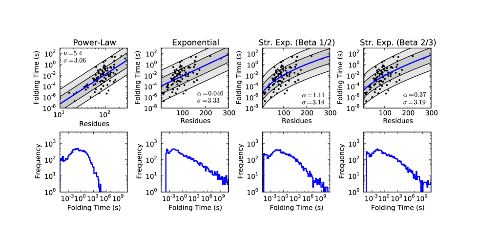
Direct fitting of all proposed models to the available data yields reasonable results for each (Fig. 1). Each model reports a scale parameter ($\sigma$) of approximately 3, which indicates that 68% of proteins will have folding times within a factor of $e^{\sigma}\approx 20$ from the time predicted by the rate law, and 95% will be within a factor of $e^{2\sigma}\approx 400$. Since the available data spans folding times of more than 9 orders of magnitude (between $1.9\cdot 10^{-7}$ and $9.9\cdot 10^{2}$ seconds), this demonstrates that chain length captures the majority of variation in folding times, since orthogonal factors (topology, mutations, etc.) account for approximately $400^{2}\sim 10^{5}$ orders of magnitude of variation.

Do the data support any one model? The power-law model is slightly favored by comparing the likelihoods that each model generated the observed data (Table 1). In such comparisons, typically a ratio of $10^{2}$ or greater is considered significant, and often models differ by hundreds of orders of magnitude Kass and Rafterty (1995) – thus, the power law model is better supported by the data, but only by a modest margin. Further, an attempt to fit the stretched exponential form with $\beta$ as a variable parameter resulted in an unreasonably small value of $\beta$ along with a very large value of $\alpha$, resulting in a fit that is very close to the power law (SI Fig. 3). Finally, the power law model has the smallest fit $\sigma$, indicating that it explains the most variation in the data, and attributes less to orthogonal factors.

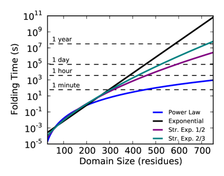
It is clear, however, that there is little difference between the models in the range of available data. These models diverge significantly only for very large proteins (Fig. 2).

Figure 2: The predicted folding times from each model in Figure 1, in a direct comparison. Intuitive timescales are denoted for clarity.

They yield significantly different predictions for the distribution of folding times, generated by transforming the known distribution of domain sizes into each of the different models (Fig. 1). The most significant differences are in the tails of these distributions, where the exponential forms predict much longer folding times for the largest proteins (Table 2).

Table 2: Estimated Fraction of Protein Domains with Folding Times Greater than Time Indicated

	Hour	Day	Month	Year
Power Law	0.41%	0.01%	0.00%	0.00%
Exponential	9.56%	5.70%	3.34%	2.46%
S. E. 1/2	5.48%	2.37%	0.95%	0.57%
S. E. 2/3	7.49%	3.53%	1.74%	1.11%

The power law model predicts no proteins fold in times longer than an hour, while the exponential forms show a significant number of proteins with folding times longer than a day (Fig. 2).

An evaluation of the reasonableness of these folding time distributions is provided by the critical time $\tau_{c}$ for each model (SI Table III). For reasonable values of $C$, the power law $\tau_{c}$ is on the order of minutes. The exponential forms, on the other hand, predict $\tau_{c}$ is on the order of hours.

Figure 3: The of probability of observing the observed domain sizes (SI Fig. 1) given a rate scaling law and a folding complexity cutoff time, $\tau_{c}$. Assumes the Gaussian model (with $C=0.10$) described in the main text. Note the y-axis is $\log_{10}$ and divided by $10^{3}$ for clarity, so small differences on the plot are actually quite large.

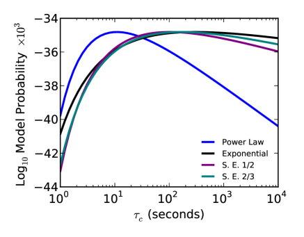
Indeed, picking a reasonable value of $\tau_{c}$ and calculating the probability of observing the empirically observed domain size distribution (Fig. 3) shows that for values of $\tau_{c}\sim 10$ seconds, the power law model is clearly the best. However, for any values of $\tau_{c}$ greater than $100$ seconds, the exponential laws are much better models.

IV Conclusions

Thus, we have a mixed conclusion. While the power law model appears to best explain the available raw data, it results in very fast predicted folding times. The exponential forms, while doing a marginally poorer job of explaining the raw data, yield a distribution of folding times much more in line with what we expect from biology. Given the current available data, no clear victor emerges.

Previous theories have claimed that simply predicting one of the four laws investigated here is strong evidence in support of that theory. This is manifestly not the case – not only must the proposed law be reasonable, but it must also predict reasonable parameter estimates, and even then the supporting evidence the rate scaling law can provide given current data is limited. Conversely, the analytical theories mentioned here are not ruled out by the current available data. This is most striking in the case of the exponential form, since exponential scaling of the folding times has often been associated with Levinthal’s paradox. This study shows that exponential scaling is reasonable given current experimental data, so long as the exponential scaling constant ($\alpha$) is sufficiently small.

Clear evidence for any one rate law remains missing, however with a few clear examples of very large globular proteins (500 residues or larger) capable of folding unassisted in vitro, it might be possible to discriminate between the models proposed here. Figure 2 clearly shows the divergences between predicted folding times for large proteins, and shows how just a few data points in this extreme regime might be able to begin differentiating between the proposed models investigated here.

References

- Thirumalai (1995) D. Thirumalai, J Phys I 5, 1457 (1995).
- Gutin et al. (1996) A. M. Gutin, V. I. Abkevich, and E. I. Shakhnovich, Phys. Rev. Lett. 77, 5433 (1996).
- Levinthal (1969) C. Levinthal, Mossbauer Spectroscopy in Biological Systems Proceedings of a meeting held at Allerton House , 22 (1969).
- Bogatyreva et al. (2009) N. S. Bogatyreva, A. A. Osypov, and D. N. Ivankov, Nucleic Acids Research 37, D342 (2009).
- Plaxco et al. (1998) K. W. Plaxco, K. T. Simons, and D. Baker, Journal of Molecular Biology 277, 985 (1998).
- Nakamura and Takano (2005) H. Nakamura and M. Takano, Phys. Rev. E 71 (2005).
- Ivankov et al. (2003) D. N. Ivankov, S. O. Garbuzynskiy, E. Alm, K. W. Plaxco, D. Baker, and A. V. Finkelstein, Protein Science 12, 2057 (2003).
- Lawrence et al. (2010) C. Lawrence, J. Kuge, K. Ahmad, and K. W. Plaxco, Journal of Molecular Biology 403, 446 (2010).
- Cieplak and Hoang (2003) M. Cieplak and T. X. Hoang, Biophys. J. 84, 475 (2003).
- Cieplak et al. (1999) M. Cieplak, T. Hoang, and M. Li, Phys. Rev. Lett. 83, 1684 (1999).
- Lane and Pande (2012) T. J. Lane and V. S. Pande, J. Phys. Chem. B , 120411093425008 (2012).
- Zwanzig et al. (1992) R. Zwanzig, A. Szabo, and B. Bagchi, Proc. Natl. Acad. Sci. 89, 20 (1992).
- Zwanzig (1995) R. Zwanzig, Proc. Natl. Acad. Sci. 92, 9801 (1995).
- Li et al. (2002) M. S. Li, D. K. Klimov, and D. Thirumalai, J. Phys. Chem. B 106, 8302 (2002).
- Naganathan and Muñoz (2005) A. N. Naganathan and V. Muñoz, J. Am. Chem. Soc. 127, 480 (2005).
- Koga and Takada (2001) N. Koga and S. Takada, Journal of Molecular Biology 313, 171 (2001).
- Finkelstein et al. (2007) A. V. Finkelstein, D. N. Ivankov, S. O. Garbuzynskiy, and O. V. Galzitskaya, Curr. Protein Pept. Sci. 8, 521 (2007).
- Wolynes (1997) P. Wolynes, Proc. Natl. Acad. Sci. 94, 6170 (1997).
- Ouyang and Liang (2008) Z. Ouyang and J. Liang, Protein Science 17, 1256 (2008).
- De Sancho and Muñoz (2011) D. De Sancho and V. Muñoz, Phys. Chem. Chem. Phys. 13, 17030 (2011).
- Ivankov and Finkelstein (2010) D. N. Ivankov and A. V. Finkelstein, J. Phys. Chem. B 114, 7930 (2010).
- Hartl and Hayer-Hartl (2009) F. U. Hartl and M. Hayer-Hartl, Nat Struct Mol Biol 16, 574 (2009).
- Xu and Nussinov (1998) D. Xu and R. Nussinov, Fold Des 3, 11 (1998).
- Shen et al. (2005) M.-y. Shen, F. P. Davis, and A. Sali, Chemical Physics Letters 405, 224 (2005).
- Kass and Rafterty (1995) R. E. Kass and A. E. Rafterty, J Am Stat Assoc 90, 773 (1995).