Matrix product states for quantum metrology

Abstract

We demonstrate that the optimal states in lossy quantum interferometry may be efficiently simulated using low rank matrix product states. We argue that this should be expected in all realistic quantum metrological protocols with uncorrelated noise and is related to the elusive nature of the Heisenberg precision scaling in the asymptotic limit of large number of probes.

Over the recent years, advancements in quantum engineering have pushed non-classical concepts such as entanglement and squeezing, previously regarded as largely academic topics, close to practical applications. Quantum features of light and atoms helped to improve the performance of measuring devices that operate in the regime where the precision is limited by the fundamental laws of physics Giovanetti . One of the most spectacular examples of practical applications of quantum metrology can be found in gravitational wave detectors LIGO , where the original idea Caves of employing squeezed states of light to improve the sensitivity of an interferometer has found its full scale realization GEO ; GEO2011 . No less impressive are experiments with trapped entangled ions demonstrating spectroscopic resolution enhancement crucial for the operation of the atomic clocks clock ; Schmidt ; Ospelkaus .

When standard sources of laser light are being used, any interferometric experiment may be fully described by treating each photon individually and claiming that each photon interferes only with itself. Sensing a phase delay $\phi$ between the two arms of the interferometer via intensity measurements may be regarded as many independent repetitions of single photon interferometric experiments. $N$ independent experiments result in the data that allows the parameter $\phi$ to be estimated with error scaling as $1/\sqrt{N}$—the so called standard quantum limit or the shot noise limit. If, however, an experiment cannot be split into $N$ independent processes, as is e.g. the case with the $N$ probing photons being entangled, the above reasoning is invalid and one can in principle achieve the $1/N$ estimation precision—the Heiseberg scaling Giovanetti2004 ; Berry ; Lee ; Zwierz — with the help of e.g. the N00N states Dowling .

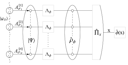
Figure 1: Quantum metrology with matrix product states. $N$ parallel quantum channels act on the input state $|\Psi\rangle$ inscribing parameter value $\phi$ as well as causing local decoherence on each of the probes. Measurement $\hat{\Pi}_{x}$ on the output state $\hat{\rho}_{\phi}$ allows to make an estimate $\tilde{\phi}(x)$ based on the measurement result $x$. The input state is a matrix product state obtained by the action of maps $A^{[k]}_{\sigma_{k}}$ on pairs of virtual $D$ dimensional systems prepared in such a way that the two adjacent systems corresponding to different neighboring particles are in a maximally entangled state $|\varphi_{D}\rangle$.

Still, in all realistic experimental setups, decoherence typically makes the relevant quantum features such as squeezing or entanglement die out very quickly Huelga ; Shaji . Recently, it has been rigorously shown for optical interferometry with loss Janek ; Knysh , as well as for more general decoherence models Escher ; RafalJanek:Fujiwara , that if decoherence acts independently on each of the probes one can get at best $c/\sqrt{N}$ asymptotic scaling of error—precision that is better than classical one only by a constant factor $c$ which depends on the type of decoherence and its strength. One can therefore appreciate the Heisenberg-like decrease in uncertainty only in the regime of small $N$, where the precise meaning of “small” depends on the decoherence strength Escher , and in typical cases is of the order of $10$ photons/atoms.

This indicates that in the limit of large number of probes, almost optimal performance can be achieved by dividing the probes into independent groups where only the probes from a given group are entangled among each other. Clearly, the size of the group that is needed to approach the fundamental $c/\sqrt{N}$ bound up to a given accuracy will depend on the strength of decoherence. Nevertheless, irrespectively of how small the decoherence strength is, for $N$ large enough the size of the group will saturate at some point and therefore asymptotically the optimal state may be regarded as only locally correlated.

A natural class of states efficiently representing locally correlated states are the Matrix Product States (MPSs) MPS1 ; MPS3 ; MPS4 ; MPS5 ; MPS6 , which have proved to be highly successful in simulating low-energy states of complex spin systems. Until now no attempt has been made, however, to employ MPSs for quantum metrology purposes. Establishing this connection is the essence of the present paper.

Basic quantum metrology scheme is depicted in Fig. 1. $N$ probe input state $|\Psi\rangle$ travels through $N$ parallel noisy channels $\Lambda_{\phi}$ which action is parameterized by an unknown value $\phi$. A measurement $\hat{\Pi}_{x}$ is performed on the output density matrix $\hat{\rho}_{\phi}=\Lambda_{\phi}^{\otimes N}(|\Psi\rangle\langle\Psi|)$ yielding a result $x$ with probability $p(x|\phi)=\textrm{Tr}(\hat{\rho}_{\phi}\hat{\Pi}_{x})$. The estimation procedure is completed by specifying an estimator function $\tilde{\phi}(x)$. Eventually we are left with the estimated value of the parameter, $\tilde{\phi}$, which in general will be different from $\phi$. We denote the average uncertainty of estimation by $\Delta\phi=\sqrt{\langle(\tilde{\phi}-\phi)^{2}\rangle}$. where the average is performed over different measurement results $x$. The main goal of theoretical quantum metrology is to find strategies that minimize $\Delta\phi$. For this purpose one has to find the optimal estimator, measurement and input state. This in general is a difficult task.

To simplify the problem one may resort to the quantum Cramer-Rao inequality Braunstein ; Helstrom ; Nielsen ; Paris

$$\Delta\phi\geq\frac{1}{\sqrt{kF(\hat{\rho}_{\phi}})},\quad F(\hat{\rho}_{\phi})=\textrm{Tr}(\hat{\rho}_{\phi}\hat{L}_{\phi}^{2})$$ (1)

that bounds the precision of any unbiased estimation strategy based on $k$ independent repetitions of an experiment. $F(\hat{\rho}_{\phi})$ is the Quantum Fisher Information (QFI) written in terms of $\hat{L}_{\phi}$—the so called symmetric logarithmic derivative (SLD)—defined implicitly as: $2\frac{d\hat{\rho}_{\phi}}{d\phi}=\hat{L}_{\phi}\hat{\rho}_{\phi}+\hat{\rho}_{\phi}\hat{L}_{\phi}$. For pure states the formula for QFI simplifies to $F(|\Psi_{\phi}\rangle)=4(\langle\dot{\Psi}_{\phi}|\dot{\Psi}_{\phi}\rangle-|\langle\dot{\Psi}_{\phi}|\Psi_{\phi}\rangle|^{2})$, where $|\dot{\Psi}_{\phi}\rangle=\frac{d|\Psi_{\phi}\rangle}{d\phi}$. The bound is known to be saturable in the asymptotic limit of $k\rightarrow\infty$ in the sense that there exist a measurement and an estimator that yields equality in (1). The main benefit of using QFI is that since it does not depend neither on the measurement nor on the estimator, the only remaining optimization problem is the maximization of $F(\hat{\rho}_{\phi})$ over input states.

Since the optimal states in the regime of large number of probes $N$ (not $k$) may be regarded as consisting of independent groups, the Cramer-Rao bound may be saturated even for $k=1$ provided $N$ is large enough Nielsen ; Guta . This makes the QFI an even more appealing quantity than in the decoherence-free case where some controversies arise on the practical use of the strategies based on the optimization of the QFI Anisimov ; Giovanetti2012 . Maximization of QFI over the most general input states for large $N$ may still be challenging, though, and even if successful might not provide an insight into the structure of the optimal states. This is the place where MPSs come in useful.

A general MPS of $N$ qubits is defined as

$$|\Psi\rangle_{\textrm{MPS}}=\frac{1}{\sqrt{\mathcal{N}}}\sum_{\sigma_{1}\dots\sigma_{N}=0}^{1}\textrm{Tr}(A_{\sigma_{1}}^{[1]}\dots A_{\sigma_{N}}^{[N]})|\sigma_{1}\dots\sigma_{N}\rangle,$$ (2)

where $A_{\sigma_{k}}^{[k]}$ are square complex matrices of dimension $D\times D$, $D$ is called the bond dimension and $\mathcal{N}$ is the normalization factor. In operational terms, a MPS is generated by assuming that each qubit is substituted by a pair of $D$ dimensional virtual systems. Adjacent systems corresponding to different neighboring particles are prepared in maximally entangled states $|\varphi_{D}\rangle=\frac{1}{\sqrt{D}}\sum_{\alpha=1}^{D}|\alpha,\alpha\rangle$ (Fig. 1) and maps $A_{\sigma_{k}}^{[k]}=\sum_{\alpha,\beta=1}^{D}A_{\sigma_{k},\alpha,\beta}|\sigma_{k}\rangle\langle\alpha,\beta|$ are applied to the pair of virtual systems corresponding to the $k$-th particle MPS5 .

Such a description of state is very efficient provided the bond dimension $D$ increases slowly with $N$. In a most favorable case when $D$ may be assumed to be bounded, $D<D_{\textrm{max}}$, the number of coefficients needed to specify an $N$ qubit state in the asymptotic regime of large $N$ will scale as $ND_{\textrm{max}}^{2}$ (linear in $N$), as opposed to the standard $2^{N}$ scaling. It should be noted, however, that in many quantum metrological models, in particular the ones based on the QFI, the search for the optimal input probe states may be restricted to symmetric (bosonic) states Huelga ; Escher ; Kolenderski ; Rafal:OptStates . Even though the description of a symmetric $N$ qubit pure state is efficient and requires only $N+1$ parameters, the use of MPSs may still offer a significant advantage as the symmetric MPS description involves matrices $A$ which are identical for different particles: $A^{[k]}_{\sigma}=A_{\sigma}$ and commute under the trace—$\textrm{Tr}(A_{\sigma_{1}}\dots A_{\sigma_{N}})$ does not depend on the order of matrices. Provided $D$ is asymptotically bounded or grows slowly with $N$, one can still benefit significantly from the use of MPS in the large $N$ regime.

In order to demonstrate the power of the MPS approach, we apply it to the most thoroughly analyzed and relevant model in quantum metrology—the lossy interferometer. We will not specify the nature of the physical systems (atoms, photons) but will rather refer to abstract two-level probes, with orthogonal sates $|0\rangle$, $|1\rangle$. The parameter to be estimated is the relative phase delay $\phi$ a probe experiences being in $|1\rangle$ vs. $|0\rangle$ state. The decoherence mechanism amounts to a loss of probes where each of the probes is lost independently of the others with probability $1-\eta$. As such, this is an example of a general scheme depicted in Fig. 1. Since the distinguishability of probes offers no advantage for phase estimation Rafal:OptStates we move to the symmetric state description where the general $N$ probe state reads $|\Psi\rangle=\sum_{n=0}^{N}\alpha_{n}|n,N-n\rangle$, and $|n,N-n\rangle$ represents $n$ and $N-n$ probes in states $|0\rangle$ and $|1\rangle$ respectively. The output state $\hat{\rho}_{\phi}$ can be written explicitly as:

$$\hat{\rho}_{\phi}=\sum_{l_{0}=0}^{N}\sum_{l_{1}=0}^{N-l_{0}}p_{l_{0}l_{1}}|\Psi^{l_{0}l_{1}}_{\phi}\rangle\langle\Psi^{l_{0}l_{1}}_{\phi}|$$ (3)

where

$$|\Psi^{l_{0}l_{1}}_{\phi}\rangle=\frac{1}{\sqrt{p_{l_{0}l_{1}}}}\sum_{n=l_{0}}^{N-l_{1}}\alpha_{n}e^{\mathrm{i}n\phi}\beta_{l_{0}l_{1}}^{n}|n-l_{0},N-n-l_{1}\rangle\\ \beta_{l_{0}l_{1}}^{n}(\eta)=\sqrt{B_{l_{0}}^{n}B_{l_{1}}^{N-n}},\ B_{l}^{n}={{n}\choose{l}}\eta^{n-l}(1-\eta)^{l}$$ (4)

and $p_{l_{0}l_{1}}$ is a normalization factor which can be interpreted as a probability to lose $l_{0}$, $l_{1}$ probes in states $|0\rangle$ and $|1\rangle$ respectively.

As the output state $\hat{\rho}_{\phi}$ is mixed, QFI is not explicitly given in terms of the input state parameters as it requires involved calculation of the SLD or other equivalent quantities Escher ; Toth ; Fujiwara . In general, due to convexity, QFI for a mixed state is smaller than a weighted sum of QFIs for pure states into which a mixed state may be decomposed. Nevertheless, it was shown in Dorner that assuming additional knowledge of how many photons were lost being in the state $|0\rangle$ and how many being in the state $|1\rangle$ does not improve the estimation precision appreciably. Hence, one can approximate the QFI with a weighted sum of QFIs all pure states entering the mixture $\hat{\rho}_{\phi}$:

$$F(\hat{\rho}_{\phi})\lesssim\tilde{F}(\hat{\rho}_{\phi})=\sum_{l_{0}=0}^{N}\sum_{l_{1}=0}^{N-l_{0}}p_{l_{0},l_{1}}F(|\Psi^{l_{0},l_{1}}_{\phi}\rangle).$$ (5)

This approximation simplifies the calculations significantly since in our case $F(|\Psi_{\phi}^{l_{0}l_{1}}\rangle)=4(\langle\Psi_{\phi}^{l_{0}l_{1}}|\hat{n}^{2}|\Psi_{\phi}^{l_{0}l_{1}}\rangle-|\langle\Psi_{\phi}^{l_{0}l_{1}}|\hat{n}|\Psi_{\phi}^{l_{0}l_{1}}\rangle|^{2})$ with $\hat{n}$ being the the excitation number operator $\hat{n}|n,N-n\rangle=n|n,N-n\rangle$. Direct optimization of formula (5) over the input state parameters $\alpha_{n}$ involves $N+1$ variables. This approach was taken in Dorner ; Rafal:OptStates . Here we consider the class of symmetric MPSs parameterized with two diagonal (assuring commutativity) $D\times D$ matrices $A_{0}$, $A_{1}$. These MPS are parameterized with $2D$ complex numbers, instead of $N+1$, and read explicitly:

$$|\Psi\rangle_{\textrm{MPS}}=\frac{1}{\sqrt{\mathcal{N}}}\sum_{n=0}^{N}\sqrt{{{N}\choose{n}}}\textrm{Tr}(A_{0}^{n}A_{1}^{N-n})|n,N-n\rangle.$$ (6)

Thanks to the simple form of Eq (5) it is possible to compute $\tilde{F}$ directly on $A_{\sigma}$ matrices and there is no need to go back to the less efficient standard description as would be the case with the formula (1).

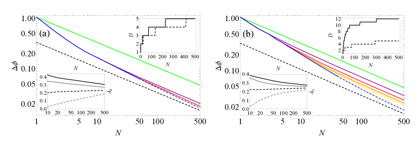
Figure 2: (color online) Log-Log plots of the phase estimation precision with losses ($\eta=0.9$) as a function of number of probes $N$ optimized over input states in (a) the QFI approach where $\Delta\phi=\frac{1}{\sqrt{F}}$ with $F$ given by Eq. (5) and (b) the Ramsey interferometry with $\Delta\phi$ given by Eq. (7). The color curves correspond to matrix product states of different bond dimensions $D$: $D=1$ (green, no correlations: $\Delta\phi=1/\sqrt{\eta N}$), $D=2$ (purple), $D=3$ (red), $D=4$ (orange), $D=5$ (yellow). The blue curves correspond to the optimal states obtained with brute force optimization, with extrapolation for higher $N$ (dashed) obtained using scaling formulas of Knysh (a) and optimization over the spin-squeezed states Ma (b). The black line represents the asymptotic bound $\Delta\phi=\sqrt{\frac{1-\eta}{\eta N}}$ Janek ; Knysh ; Escher ; RafalJanek:Fujiwara . The upper-right insets depict the bond dimension $D$ needed to reach the optimal precision with at most $1\%$ discrepancy: $\eta=0.9$ (solid), $\eta=0.3$ (dashed). Lower-left insets present normalized absolute values of elements of the optimal diagonal MPS matrix $A_{\sigma}$ for bond dimension $D=4$ and $\eta=0.9$.

Fig. 2a illustrates the precision obtained using MPS for the case of relatively small losses $\eta=0.9$. As one can see, the MPS approximation is excellent. In particular, the upper-right inset shows that already $D=5$ is sufficient to obtain less than $1\%$ discrepancy for $N\leq 500$. We have confirmed this observation for different $\eta$ and observed that for higher losses (lower $\eta$) lower $D$ are required to obtain a given level of approximation for a particular $N$—an effect that should be much more spectacular for larger $N$ reflecting the fact that stronger decoherence diminishes the role of quantum correlations.

Moreover we have observed that optimal matrices $A_{0}$, $A_{1}$ have the same diagonal values which are ordered complementarily—the highest in $A_{0}$ is paired with lowest one in $A_{1}$ etc. The higher is $N$ the closer the diagonal values approach each other as can be seen from the lower-left inset on Fig. (2). This confirms the intuition that with increasing $N$, the optimal states are becoming less distinct from the product state—all diagonal values of $A_{\sigma}$ equal.

The peculiarity of phase estimation is that in the decoherence-free case optimal QFI is achieved for the N00N state which, even though has non-local correlations, is an example of an MPS with $D=2$. This makes the MPS capable of approximating the optimal states very well even for low loss and small $N$ $[N\lesssim 1/(1-\eta)]$—an ability that in general will not hold for other estimation problems.

Taking now a more operational approach, not based on the QFI, one may consider a concrete measurement scheme with a particular observable $\hat{O}$ being measured. Simple error-propagation formula for $\phi$ yields $\Delta\phi=\Delta\hat{O}/|\frac{\textrm{d}\langle\hat{O}\rangle}{\textrm{d}\phi}|$. In the Ramsey spectroscopy setup Wineland1 , or equivalently in the Mach-Zehnder interferometer with photon number difference measurement, one effectively measures a component of the total angular momentum operator $\hat{J}$ of $N$ spins 1/2—if a qubit $|0\rangle$, $|1\rangle$ is treated as a spin 1/2 particle Lee . If the phase dependent rotation $\hat{U}=e^{i\phi\hat{J}_{z}}$ is being sensed by the measurement of the $\hat{J}_{x}$ observable, the explicit formula for estimation uncertainty at the optimal operation point $\phi=0$ calculated for $\hat{\rho}_{\phi}$ from Eq. (3) reads

$$\Delta\phi=\sqrt{\frac{\Delta^{2}\hat{J}_{x}}{\langle\hat{J}_{y}\rangle^{2}}+\frac{1-\eta}{\eta}\frac{N}{4\langle\hat{J}_{y}\rangle^{2}}}.$$ (7)

Search for the optimal state amounts to minimizing the above quantity. Since it depends only on first and second moments of $\hat{J}$ it is simple to implement numerically using MPS. Results are presented in Fig. 2b.

It is clear that MPS are capable to capture the essential feature of the optimal states—the squeezing of the $\hat{J}_{x}$—with relatively low bond dimensions $D$. Moreover, the upper-right inset indicates that the required bond dimension $D$ is reduced much more significantly with increasing decoherence strength than in the QFI approach. The lower-left inset confirms again that the structure of the optimal states gets closer to the product state structure with increasing $N$. We have also applied the MPS approach to Ramsey spectroscopy with other decoherence models including independent dephasing, depolarization and spontaneous emission and have obtained completely analogous results.

In summary, we have shown that MPS are very well suited for achieving the optimal performance in realistic quantum metrological setups and may reduce the numerical effort while searching for the optimal estimation strategies. Even though we have based our presentation on a single model of lossy phase estimation we anticipate these conclusions to be valid in all metrological setups where decoherence makes the asymptotic Heisenberg scaling unachievable—the intuitive argument being that no large scale strong correlations are needed to reach the optimal performance. An intriguing open question remains: is it possible, as it is in many-body physics problems, to obtain an exponential reduction in numerical complexity thanks to the use of MPS. This is not possible when the optimal states are known to be symmetric, as in the lossy phase estimation. In problems, however, where distinguishability of probes is essential as e.g. in Bayesian multiparameter estimation Chiribella ; Bagan , MPS might demonstrate their full potential when impact of decoherence is taken into account.

We thank Janek Kołodyński and Konrad Banaszek for fruitful discussions and support. This research was supported by the European Commission under the Integrating Project Q-ESSENCE, Polish NCBiR under the ERA-NET CHIST-ERA project QUASAR and the Foundation for Polish Science under the TEAM programme.

References

- (1) V. Giovanetti, S. Lloyd and L. Maccone, Nature Photon. 5, 222 (2011)
- (2) B. P. Abbott et al., Rep. Prog. Phys. 72, 076901 (2009).
- (3) C. M. Caves, Phys. Rev. D 23, 1693 (1981)
- (4) J. Abadie et al. (The Ligo Scientific Collaboration), Nature Phys. 7, 962, (2011)
- (5) Henning Vahlbruch et al., Class. Quantum Grav. 27, 084027 (2010).
- (6) J. J. Bollinger, W. M. Itano, D. J. Wineland, and D. J. Heinzen, Phys. Rev. A 54, R4649 (1996).
- (7) P. O. Schmidt, T. Rosenband, C. Langer, W. M. Itano, J. C. Bergquist and D. J. Wineland, Science 309, 749 (2005)
- (8) C. Ospelkaus, U. Warring, Y. Colombe, K. R. Brown, J. M. Amini, D. Leibfried and D. J. Wineland, Nature 476, 181 (2011)
- (9) V. Giovannetti, S. Lloyd, L. Maccone, Science 306, 1330 2004).
- (10) D. W. Berry, H. M. Wiseman, Phys. Rev. Lett. 85, 5098 (2000).
- (11) H. Lee, P. Kok, J. P. Dowling, J. Mod. Opt. 49, 2325 (2002).
- (12) M. Zwierz, C. A. Perez-Delgado and P. Kok, Phys. Rev. Lett. 105, 180402 (2010)
- (13) J. P. Dowling, Phys. Rev. A 57, 4736 (1998)
- (14) S. F. Huelga et. al., Phys. Rev. Lett. 79, 3865 (1997)
- (15) A. Shaji and C. M. Caves, Phys. Rev. A 76, 032111 (2007)
- (16) S. Knysh, V. N. Smelyanskiy and G. A. Durkin, Phys. Rev. A 83, 021804(R) (2011)
- (17) J. Kolodynski and R. Demkowicz-Dobrzanski, Phys. Rev. A 82, 053804 (2010)
- (18) B. M. Escher, R. L. de Matos Filho, L. Davidovich, Nature Physics 7, 406-411 (2011).
- (19) R. Demkowicz-Dobrzański, J. Kolodyński, M. Guta, Nature Communications 3, 1063 (2012).
- (20) I. Affleck, T. Kennedy, E. H. Lieb, H. Tasaki, Commun. Math. Phys. 115, 477 (1988).
- (21) M. Fannes, B. Nachtergaele, R. F. Werner, Commun. Math. Phys. 144, 443-490 (1992).
- (22) F. Verstraete, J. I. Cirac, Phys. Rev. B 73, 094423 (2006).
- (23) D. Perez-Garcia, F. Verstraete, M. M. Wolf, J. I. Cirac, Quantum Inf. Comput. 7, 401 (2007)
- (24) F. Verstraete, J. I. Cirac and V. Murg, Adv. Phys. 57, 143 (2008)
- (25) S. L. Braunstein, C. M. Caves, Phys. Rev. Lett. 72, 3439 (1994).
- (26) C. W. Helstrom, Quantum Detection and Estimation Theory, Academic Press, 1976.
- (27) O. E. Barndorff-Nielsen, R. D. Gill, P. E. Jupp, J. R. Statist. Soc. B, 65, 775-816 (2003).
- (28) M. G. A. Paris, Int. J. Quant. Inf. 7, 125 (2009)
- (29) J. Kahn and M. Guta, Commun. Math. Phys. 289, 597 652 (2009).
- (30) P. Anisimov et al. Phys. Rev. Lett. 104, 103602 (2010).
- (31) V. Giovannetti and L. Maccone, Phys. Rev. Lett. 108, 210404 (2012)
- (32) P. Kolenderski, R. Demkowicz-Dobrzański, Phys. Rev. A 78, 052333 (2008).
- (33) R. Demkowicz-Dobrzański et al., Phys. Rev. A 80, 013825 (2009).
- (34) Géza Tóth, Dénes Petz, Phys. Rev. A 87, 032324 (2013).
- (35) A. Fujiwara, H. Imai, J. Phys. A: Math. Theor. 41, 255304 (2008).
- (36) U. Dorner et al., Phys. Rev. Lett. 102, 040403 (2009)
- (37) D. J. Wineland, J. J. Bollinger, W. M. Itano, F. L. Moore, D. J. Heinzen, Phys. Rev. A 46, R6797 (1992).
- (38) J. Ma, X. Wang, C. P. Sun and F. Nori, Phys. Rep. 509, 89 (2011)
- (39) G. Chiribella, G. M. D’Ariano, P. Perinotti and M. F. Sacchi, Phys. Rev. Lett. 93, 180503 (2004)
- (40) E. Bagan, M. Baig, A. Brey, R. Munoz-Tapia and R. Tarrach, Phys. Rev. A 63, 052309 (2001)