Graphical Models via Univariate
Exponential Family Distributions

Abstract

Undirected graphical models, or Markov networks, are a popular class of statistical models, used in a wide variety of applications. Popular instances of this class include Gaussian graphical models and Ising models. In many settings, however, it might not be clear which subclass of graphical models to use, particularly for non-Gaussian and non-categorical data. In this paper, we consider a general sub-class of graphical models where the node-wise conditional distributions arise from exponential families. This allows us to derive multivariate graphical model distributions from univariate exponential family distributions, such as the Poisson, negative binomial, and exponential distributions. Our key contributions include a class of M-estimators to fit these graphical model distributions; and rigorous statistical analysis showing that these M-estimators recover the true graphical model structure exactly, with high probability. We provide examples of genomic and proteomic networks learned via instances of our class of graphical models derived from Poisson and exponential distributions.

Keywords: Graphical Models, Model Selection, Sparse Estimation

1 Introduction

Undirected graphical models, also known as Markov random fields, are an important class of statistical models that have been extensively used in a wide variety of domains, including statistical physics, natural language processing, image analysis, and medicine. The key idea in this class of models is to represent the joint distribution as a product of clique-wise compatibility functions. Given an underlying graph, each of these compatibility functions depends only on a subset of variables within any clique of the underlying graph. Popular instances of such graphical models include Ising and Potts models (see references in Wainwright and Jordan (2008) for a varied set of applications in computer vision, text analytics, and other areas with discrete variables), as well as Gaussian Markov Random Fields (GMRFs), which are popular in many scientific settings for modeling real-valued data. A key modeling question that arises, however, is: how do we pick the clique-wise compatibility functions, or alternatively, how do we pick the form or sub-class of the graphical model distribution (e.g. Ising or Gaussian MRF)? For the case of discrete random variables, Ising and Potts models are popular choices; but these are not best suited for count-valued variables, where the values taken by any variable could range over the entire set of positive integers. Similarly, in the case of continuous variables, Gaussian Markov Random Fields (GMRFs) are a popular choice; but the distributional assumptions imposed by GMRFs are quite stringent. The marginal distribution of any variable would have to be Gaussian for instance, which might not hold in instances when the random variables characterizing the data are skewed (Liu et al., 2009). More generally, Gaussian random variables have thin tails, which might not capture fat-tailed events and variables. For instance, in the finance domain, the lack of modeling of fat-tailed events and probabilities has been suggested as one of the causes of the 2008 financial crisis (Acemoglu, 2009).

To address this modeling question, some have recently proposed non-parametric extensions of graphical models. Some, such as the non-paranormal (Liu et al., 2009; Lafferty et al., 2012) and copula-based methods (Dobra and Lenkoski, 2011; Liu et al., 2012a), use or learn transforms that Gaussianize the data, and then fit Gaussian MRFs to estimate network structure. Others, use non-parametric approximations, such as rank-based estimators, to the correlation matrix, and then fit a Gaussian MRF (Xue and Zou, 2012; Liu et al., 2012b). More broadly, there could be non-parametric methods that either learn the sufficient statistics functions, or learn transformations of the variables, and then fit standard MRFs over the transformed variables. However, the sample complexity of such classes of non-parametric methods is typically inferior to those that learn parametric models. Alternatively, and specifically for the case of multivariate count data, Lauritzen (1996); Bishop et al. (2007) have suggested combinatorial approaches to fitting graphical models, mostly in the context of contingency tables. These approaches, however, are computationally intractable for even moderate numbers of variables.

Interestingly, for the case of univariate data, we have a good understanding of appropriate statistical models to use. In particular, a count-valued random variable can be modeled using a Poisson distribution; call-times, time spent on websites, diffusion processes, and life-cycles can be modeled with an exponential distribution; other skewed variables can be modeled with gamma or chi-squared distributions. Here, we ask if we can extend this modeling toolkit from univariate distributions to multivariate graphical model distributions? Interestingly, recent state of the art methods for learning Ising and Gaussian MRFs (Meinshausen and Bühlmann, 2006; Ravikumar et al., 2010; Jalali et al., 2011) suggest a natural procedure deriving such multivariate graphical models from univariate distributions. The key idea in these recent methods is to learn the MRF graph structure by estimating node-neighborhoods, or by fitting node-conditional distributions of each node conditioned on the rest of the nodes. Indeed, these node-wise fitting methods have been shown to have strong computational as well as statistical guarantees. Here, we consider the general class of models obtained by the following construction: suppose the node-conditional distributions of each node conditioned on the rest of the nodes follows a univariate exponential family. By the Hammersley-Clifford Theorem (Lauritzen, 1996), and some algebra as derived in Besag (1974), these node-conditional distributions entail a global multivariate distribution that (a) factors according to cliques defined by the graph obtained from the node-neighborhoods, and (b) has a particular set of compatibility functions specified by the univariate exponential family. The resulting class of MRFs, which we call exponential family MRFs, broadens the class of models available off the shelf, from the standard Ising, indicator-discrete, and Gaussian MRFs.

Thus the class of exponential family MRFs provides a principled approach to model multivariate distributions and network structures among a large number of variables; by providing a natural way to “extend” univariate exponential families of distributions to the multivariate case, in many cases where multivariate extensions did not exist in an analytical or computationally tractable form. Potential applications for these exponential family graphical models abound. Networks of call-times, time spent on websites, diffusion processes, and life-cycles can be modeled with exponential graphical models; other skewed multivariate data can be modeled with gamma or chi-squared graphical models; while multivariate count data such as from website visits, user-ratings, crime and disease incident reports, and bibliometrics could be modeled via Poisson graphical models. A key motivating application for our research is multivariate count data from next-generation genomic sequencing technologies (Mortazavi et al., 2008). This technology produces read counts of the number of short RNA fragments that have been mapped back to a particular gene; and measures gene expression with less technical variation than, and is thus rapidly replacing, microarrays (Marioni et al., 2008). Univariate count data is typically modeled using Poisson or negative binomial distributions (Li et al., 2011). As Gaussian graphical models have been traditionally used to understand genomic relationships and estimate regulatory pathways from microarray data, Poisson and negative-binomial graphical models could thus be used to analyze this next-generation sequencing data. Furthermore, there is a proliferation of new technologies to measure high-throughput genomic variation in which the data is not even approximately Gaussian (single nucleotide polymorphisms, copy number, methylation, and micro-RNA and gene expression via next-generation sequencing). For this data, a more general class of high-dimensional graphical models could thus lead to important breakthroughs in understanding genomic relationships and disease networks.

The construction of the class of exponential family graphical models also suggests a natural method for fitting such models: node-wise neighborhood estimation via sparsity constrained node-conditional likelihood maximization. A main contribution of this paper is to provide a sparsistency analysis (or analysis of variable selection consistency) for the recovery of the underlying graph structure of this broad class of MRFs. We note that the presence of non-linearities arising from the generalized linear models (GLM) posed subtle technical issues not present in the linear case (Meinshausen and Bühlmann, 2006). Indeed, for the specific cases of logistic, and multinomial respectively, Ravikumar et al. (2010); Jalali et al. (2011) derive such a sparsistency analysis via fairly extensive arguments, but which were tuned to the specific cases; for instance they used the fact that the variables were bounded, and the specific structure of the corresponding GLMs. Here we generalize their analysis to general GLMs, which required a subtler analysis as well as a slightly modified M-estimator. We note that this analysis might be of independent interest even outside the context of modeling and recovering graphical models. In recent years, there has been a trend towards unified statistical analyses that provide statistical guarantees for broad classes of models via general theorems (Negahban et al., 2012). Our result is in this vein and provides structure recovery for the class of sparsity constrained generalized linear models. We hope that the techniques we introduce might be of use to address the outstanding question of sparsity constrained M-estimation in its full generality.

There has been related work on the simple idea above of constructing joint distributions via specifying node-conditional distributions. Varin and Vidoni (2005); Varin et al. (2011) propose the class of composite likelihood models where the joint distribution is a function of the conditional distributions of subsets of nodes conditioned on other subsets. Besag (1974) discuss such joint distribution constructions in the context of node-conditional distributions belonging to exponential families, but for special cases of joint distributions such as pairwise models. In this paper, we consider the general case of higher-order graphical models for the joint distributions, and univariate exponential families for the node-conditional distributions. Moreover, a key contribution of the paper is that we provide tractable $M$-estimators with corresponding high-dimensional statistical guarantees and analysis for learning this class of graphical models even under high-dimensional statistical regimes.

Additionally, we note that a preliminary abridged version of this paper appeared at (Yang et al., 2012). In this manuscript, we provide a more in depth theoretical analysis along with several novel developments. Particularly, we provide a novel analytic framework on the sparsistency of our $M$-estimators that provide tighter finite-sample bounds, simpler proofs, and less restrictive assumptions than that of (Yang et al., 2012); these innovations are discussed further in Section 3.2. Further, we highlight and study several instances of our framework, relating our work to the existing literature on Gaussian MRFs and Ising models, as well as introducing two novel instances, the Poisson MRF and Exponential MRF. For each of these cases, we provide specific corollaries on conditions necessary for sparsistent recovery of the underlying graph structure. Finally, we also provide a greatly expanded experimental analysis of our class of MRFs and their $M$-estimators compared to that of (Yang et al., 2012). Focusing on two novel instances of our model, the Poisson and Exponential MRF, we study the theoretical rates, graph structural recovery, and robustness of our estimators through simulated examples. Further, we provide an additional case study on protein signaling networks using the Exponential MRF in Section 4.2.2.

2 Exponential Family Graphical Models

Suppose $X=(X_{1},\ldots,X_{p})$ is a random vector, with each variable $X_{i}$ taking values in a set $\mathcal{X}$. Let $G=(V,E)$ be an undirected graph over the set of nodes $V:=\{1,\ldots,p\}$ corresponding to the $p$ variables $\{X_{r}\}_{r=1}^{p}$. The graphical model over $X$ corresponding to $G$ is a set of distributions that satisfy Markov independence assumptions with respect to the graph $G$ (Lauritzen, 1996). By the Hammersley-Clifford theorem (Clifford, 1990), any such distribution that is strictly positive over its domain also factors according to the graph in the following way. Let $\mathcal{C}$ be a set of cliques (fully-connected subgraphs) of the graph $G$, and let $\{\phi_{c}(X_{c})\}_{c\in\mathcal{C}}$ be a set of clique-wise sufficient statistics. With this notation, any strictly positive distribution of $X$ within the graphical model family represented by the graph $G$ takes the form:

$$P(X) \propto \exp\biggr{\{}\sum_{c\in\mathcal{C}}\theta_{c}\phi_{c}(X_{c})\biggr{\}},$$ (1)

where $\{\theta_{c}\}$ are weights over the sufficient statistics. An important special case is a pairwise graphical model, where the set of cliques $\mathcal{C}$ consists of the set of nodes $V$ and the set of edges $E$, so that

$$P(X) \propto \exp\biggr{\{}\sum_{r\in V}\theta_{r}\phi_{r}(X_{r})+\sum_{(r,t)\in E}\theta_{rt}\phi_{rt}(X_{r},X_{t})\biggr{\}}.$$ (2)

As previously discussed, an important question is how to select the form of the graphical model distribution, which under the above parametrization in (1), translates to the question of selecting the class of sufficient statistics, $\phi$. As discussed in the introduction, it is of particular interest to derive such a graphical model distribution as a multivariate extension of specified univariate parametric distributions such as negative binomial, Poisson, and others. We next outline a subclass of graphical models that answer these questions via the simple construction: set the node-conditional distributions of each node conditioned on the rest of the nodes as following a univariate exponential family, and then derive the joint distribution that is consistent with these node-conditional distributions. Then, in Section 3, we will study how to learn the underlying graph structure, or the edge set $E$, for this general class of “exponential family” graphical models. We provide a natural sparsity-encouraging $M$-estimator, and sufficient conditions under which the $M$-estimator recovers the graph structure with high probability.

2.1 The Form of Exponential Family Graphical Models

A popular class of univariate distributions is the exponential family, whose distribution for a random variable $Z$ is given by

$$P(Z)=\exp\Big{\{}\theta\,B(Z)+C(Z)-D(\theta)\Big{\}},$$ (3)

with sufficient statistics $B(Z)$, base measure $C(Z)$, and log-normalization constant $D(\theta)$. Such exponential family distributions include a wide variety of commonly used distributions such as Gaussian, Bernoulli, multinomial, Poisson, exponential, gamma, chi-squared, beta, and many others; any of which can be instantiated with particular choices of the functions $B(\cdot)$, and $C(\cdot)$. Such exponential family distributions are thus used to model a wide variety of data types including skewed continuous data and count data. Here, we ask if we can leverage this ability to model univariate data to also model the multivariate case. Let $X=(X_{1},X_{2},\ldots,X_{p})$ be a $p$-dimensional random vector; and let $G=(V,E)$ be an undirected graph over $p$ nodes corresponding to the $p$ variables. Could we then derive a graphical model distribution over $X$ with underlying graph $G$, from a particular choice of univariate exponential family distribution (3) above?

Consider the following construction. Set the distribution of $X_{r}$ given the rest of nodes $X_{V\backslash r}$ to be given by the above univariate exponential family distribution (3), and where the canonical exponential family parameter $\theta$ is set to a linear combination of $k$-th order products of univariate functions $\{B(X_{t})\}_{t\in N(r)}$, where $N(r)$ is the set of neighbors of node $r$ according to graph $G$. This gives the following conditional distribution:

$$P(X_{r}|X_{V\backslash r}) =\exp\bigg{\{}B(X_{r})\Big{(}\theta_{r}+\sum_{t\in N(r)}\theta_{rt}\,B(X_{t})+\sum_{t_{2},t_{3}\in N(r)}\theta_{r\,t_{2}t_{3}}\,B(X_{t_{2}})B(X_{t_{3}})$$

$$+\ldots+\sum_{t_{2},\ldots,t_{k}\in N(r)}\theta_{r\,t_{2}\ldots t_{k}}\,\prod_{j=2}^{k}B(X_{t_{j}})\Big{)}+C(X_{r})-\bar{D}(X_{V\backslash r})\bigg{\}},$$ (4)

where $C(X_{r})$ is specified by the exponential family, and $\bar{D}(X_{V\backslash r})$ is the log-normalization constant. Notice that we use the notation $\bar{D}(\cdot)$ in case when we express the log-partition function in terms of random variables. That is, $\bar{D}(X_{V\backslash r}):=D\big{(}\theta(X_{V\backslash r})\big{)}$ where $\theta(X_{V\backslash r})$ is the canonical parameter $\theta$ derived from $X_{V\backslash r}$.

By the Hammersley-Clifford theorem, and some elementary calculation, this conditional distribution can be shown to specify the following unique joint distribution $P(X_{1},\ldots,X_{p})$:

Proposition 1

Suppose $X=(X_{1},X_{2},\ldots,X_{p})$ is a $p$-dimensional random vector, and its node-conditional distributions are specified by (2.1) given an undirected graph $G$. Then its joint distribution $P(X_{1},\ldots,X_{p})$ belongs to the graphical model represented by $G$, and is given by:

$$P(X) =\exp\Biggr{\{}\sum_{r\in V}\theta_{r}B(X_{r})+\sum_{r\in V}\sum_{t\in N(r)}\theta_{rt}\,B(X_{r})B(X_{t})+\ldots$$

$$+\sum_{r\in V}\sum_{t_{2},\ldots,t_{k}\in N(r)}\theta_{r\ldots t_{k}}\,B(X_{r})\prod_{j=2}^{k}B(X_{t_{j}})+\sum_{r\in V}C(X_{r})-A(\theta)\Biggr{\}},$$ (5)

where $A(\theta)$ is the log-normalization constant.

Note that the function $D(\cdot)$ (and hence $\bar{D}(\cdot)$) in (2.1) is the log-partition function of the node-conditional distribution, while the function $A(\cdot)$ in (1) in turn is the log-partition function of the joint distribution. Proposition 1, thus, provides an answer to our earlier question on selecting the form of a graphical model distribution given a univariate exponential family distribution. When the node-conditional distributions follow a univariate exponential family as in (2.1), there exists a unique graphical model distribution as specified by (1). One question that remains, however, is whether the above construction, beginning with (2.1), is the most general possible. In particular, note that the canonical parameter of the node-conditional distribution in (2.1) is a tensor factorization of the univariate sufficient statistic, which seems a bit stringent. Interestingly, by extending the argument from (Besag, 1974), which considers the special pairwise case, and the Hammersley-Clifford Theorem, we can show that indeed (2.1) and (1) have the most general form.

Theorem 2

Suppose $X=(X_{1},X_{2},\ldots,X_{p})$ is a $p$-dimensional random vector, and its node-conditional distributions are specified by an exponential family,

$$P(X_{r}|X_{V\backslash r})=\exp\Big{\{}E(X_{V\backslash r})\,B(X_{r})+C(X_{r})-\bar{D}(X_{V\backslash r})\Big{\}},$$ (6)

where the function $E(X_{V\backslash r})$, the canonical parameter of exponential family, depends on the rest of all random variables except $X_{r}$ (and hence the log-normalization constant $\bar{D}(X_{V\backslash r})$). Further, suppose the corresponding joint distribution factors according to the graph $G$, with the factors over cliques of size at most $k$. Then, the conditional distribution in (6) necessarily has the tensor-factorized form in (2.1), and the corresponding joint distribution has the form in (1).

Theorem 2 thus tells us that under the general assumptions that:

(a)

the joint distribution is a graphical model that factors according to a graph $G$, and has clique-factors of size at most $k$, and

(b)

its node-conditional distribution follows an exponential family,

it necessarily follows that the conditional and joint distributions are given by (2.1) and (1) respectively.

An important special case is when the joint graphical model distribution has clique factors of size at most two. From Theorem 2, the conditional distribution is given by:

$$P(X_{r}|X_{V\backslash r})=\exp\bigg{\{}\theta_{r}\,B(X_{r})+\sum_{t\in N(r)}\theta_{rt}\,B(X_{r})B(X_{t})+C(X_{r})-\bar{D}(X_{V\backslash r})\bigg{\}},$$ (7)

while the joint distribution is given as:

$$P(X)=\exp\bigg{\{}\sum_{r\in V}\theta_{r}B(X_{r})+\sum_{(r,t)\in E}\theta_{rt}\,B(X_{r})B(X_{t})+\sum_{r\in V}C(X_{r})-A(\theta)\bigg{\}}.$$ (8)

For many classes of models (e.g. general Ising, discrete CRFs), the log-partition function of the joint distribution, $A(\cdot)$, has no analytical form, and might even be intractable to compute, while the function $D(\cdot)$ typically is more amenable, and available in analytical form, since it is the log-partition function of a univariate exponential family distribution.

When the univariate sufficient statistic function $B(\cdot)$ is a linear function $B(X_{r})=X_{r}$, then the conditional distribution in (7) is precisely a generalized linear model (McCullagh and Nelder, 1989) in canonical form,

$$P(X_{r}|X_{V\backslash r})=\exp\bigg{\{}\theta_{r}\,X_{r}+\sum_{t\in N(r)}\theta_{rt}\,X_{r}\,X_{t}+C(X_{r})-\bar{D}(X_{V\backslash r};\theta)\bigg{\}},$$ (9)

where the canonical parameter of GLMs becomes $\theta_{r}+\sum_{t\in N(r)}\theta_{rt}\,X_{t}$. At the same time, the joint distribution has the form

$$P(X)=\exp\bigg{\{}\sum_{r\in V}\theta_{r}X_{r}+\sum_{(r,t)\in E}\theta_{rt}\,X_{r}\,X_{t}+\sum_{r\in V}C(X_{r})-A(\theta)\bigg{\}},$$ (10)

where the log-partition function $A(\cdot)$ in this case is defined as

$$A(\theta):=\log\int_{X}\exp\bigg{\{}\sum_{r\in V}\theta_{r}X_{r}+\sum_{(r,t)\in E}\theta_{rt}\,X_{r}\,X_{t}+\sum_{r\in V}C(X_{r})\bigg{\}}dX.$$ (11)

We will now provide some examples of our general class of “exponential family” graphical model distributions, focusing on the case in (10) with linear functions $B(X_{r})=X_{r}$. For each of these examples, we will also detail the domain, $\Theta:=\{\theta:A(\theta)<+\infty\}$, of valid parameters that ensure that the density is normalizable. Indeed, such constraints on valid parameters are typically necessary for the distributions over countable discrete or continuous valued variables.

Gaussian Graphical Models.

The popular Gaussian graphical model (Speed and Kiiveri, 1986) can be derived as an instance of the construction in Theorem 2, with the univariate Gaussian distribution as the exponential family distribution. The univariate Gaussian distribution with known variance $\sigma^{2}$ is given by,

$$P(Z)\propto\exp\left\{\frac{\mu}{\sigma}\frac{Z}{\sigma}-\frac{Z^{2}}{2\sigma^{2}}\right\},$$

where $Z\in\mathbb{R}$, so that it can be seen to be an exponential family distribution of the form (3), with sufficient statistic $B(Z)=\frac{Z}{\sigma}$, and base measure $C(Z)=-\frac{Z^{2}}{2\sigma^{2}}$. Substituting these in (10), we get the distribution,

$$P(X;\theta)\propto\exp\Bigg{\{}\sum_{r\in V}\frac{1}{\sigma_{r}}\theta_{r}X_{r}+\sum_{(r,t)\in E}\frac{1}{\sigma_{r}\sigma_{t}}\theta_{rt}\,X_{r}\,X_{t}-\sum_{r\in V}\frac{X_{r}^{2}}{2\sigma_{r}^{2}}\Bigg{\}},$$ (12)

which can be seen to be the multivariate Gaussian distribution. Note that the set of parameters $\{\theta_{rt}\}_{(r,t)\in E}$ entails a precision matrix that needs to be positive definite for a valid probability distribution.

Ising Models

The Ising model (Wainwright and Jordan, 2008) in turn can be derived from the construction in Theorem 2 with the Bernoulli distribution as the univariate exponential family distribution. The Bernoulli distribution is a member of the exponential family of the form (3), with sufficient statistic $B(X)=X$, and base measure $C(X)=0$, and with variables taking values in the set $\mathcal{X}=\{0,1\}$. Substituting these in (10), we get the distribution,

$$P(X;\theta)=\exp\Bigg{\{}\sum_{(r,t)\in E}\theta_{rt}\,X_{r}\,X_{t}-A(\theta)\Bigg{\}},$$ (13)

where we have ignored the singleton term, i.e. set $\theta_{r}=0$ for simplicity. The form of the multinomial graphical model, an extension of the Ising model, can also be represented by (10) and has been previously studied in Jalali et al. (2011) and others. The Ising model imposes no constraint on its parameters, $\{\theta_{rt}\}$, for normalizability, since there are finitely many configurations of the binary random vector $X$.

Poisson Graphical Models

Poisson graphical models are an interesting instance with the Poisson distribution as the univariate exponential family distribution. The Poisson distribution is a member of the exponential family of the form (3), with sufficient statistic $B(X)=X$ and $C(X)=-\mathrm{log}(X!)$, and with variables taking values in the set $\mathcal{X}=\{0,1,2,...\}$. Substituting these in (10), we get the following Poisson graphical model distribution:

$$P(X;\theta)=\exp\Bigg{\{}\sum_{r\in V}\big{(}\theta_{r}X_{r}-\log(X_{r}!)\big{)}+\sum_{(r,t)\in E}\theta_{rt}\,X_{r}\,X_{t}-A(\theta)\Bigg{\}}.$$ (14)

For this Poisson family, with some calculation, it can be seen that the normalizability condition, $A(\theta)<+\infty$, entails $\theta_{rt}\leq 0\ \forall\ r,t$. In other words, the Poisson graphical model can only capture negative conditional relationships between variables.

Exponential Graphical Models

Another interesting instance uses the exponential distribution as the univariate exponential family distribution, with sufficient statistic $B(X)=-X$ and $C(X)=0$, and with variables taking values in $\mathcal{X}=\{0\}\cup\mathbb{R}^{+}$. Such exponential distributions are typically used for data describing inter-arrival times between events, among other applications. Substituting these in (10), we get the following exponential graphical model distribution:

$$P(X;\theta)=\exp\Bigg{\{}-\sum_{r\in V}\theta_{r}X_{r}-\sum_{(r,t)\in E}\theta_{rt}\,X_{r}\,X_{t}-A(\theta)\Bigg{\}}.$$ (15)

To ensure that the distribution is valid and normalizable, so that $A(\theta)<+\infty$, we then require that $\theta_{r}>0,\theta_{rt}\geq 0\ \forall\ r,t$. Because of the negative sufficient statistic, this implies that the exponential graphical model can only capture negative conditional relationships between variables.

3 Statistical Guarantees on Learning Graphical Model Structures

In this section, we study the problem of learning the graph structure of an underlying exponential family MRF, given i.i.d. samples. Specifically, we assume that we are given $n$ samples of random vector $X^{1:n}:=\{X^{(i)}\}_{i=1}^{n}$, from a pairwise exponential family MRF,

$$P(X;\theta^{*})=\exp\Bigg{\{}\sum_{r\in V}\theta^{*}_{r}X_{r}+\sum_{(r,t)\in E^{*}}\theta^{*}_{rt}\,X_{r}\,X_{t}+\sum_{r}C(X_{r})-A(\theta^{*})\Bigg{\}}.$$ (16)

The goal in graphical model structure recovery is to recover the edges $E^{*}$ of the underlying graph $G=(V,E^{*})$. Following Meinshausen and Bühlmann (2006); Ravikumar et al. (2010); Jalali et al. (2011), we will approach this problem via neighborhood estimation: where we estimate the neighborhood of each node individually, and then stitch these together to form the global graph estimate. Specifically, if we have an estimate $\widehat{N}(r)$ for the true neighborhood $N^{*}(r)$, then we can estimate the overall graph structure as,

$$\widehat{E}=\cup_{r\in V}\cup_{t\in\widehat{N}(r)}\{(r,t)\}.$$ (17)

Remark.

Note that the node-neighborhood estimates $\widehat{N}(r)$ might not be symmetric (i.e. there may be a pair $(r,s)\in V\times V$, with $r\in\widehat{N}(s)$, but $s\not\in\widehat{N}(r)$). The graph-structure estimate in (17) provides one way to reconcile these neighborhood estimates; see Meinshausen and Bühlmann (2006) for some other ways to do so (though as they note, these different estimates have asymptotically identical sparsistency guarantees: given exponential convergence in the probability of node-neighborhood recovery to one, the probability that the node-neighborhood estimates are symmetric, and hence that the different “reconciling” graph estimates would become identical, also converges to one.)

The problem of graph structure recovery can thus be reduced to the problem of recovering the neighborhoods of all the nodes in the graph. In order to estimate the neighborhood of any node in turn, we consider the sparsity constrained conditional MLE. Note that given the joint distribution in (16), the conditional distribution of $X_{r}$ given the rest of the nodes is reduced to a GLM and given by,

$$P(X_{r}|X_{V\backslash r})=\exp\Bigg{\{}X_{r}\Big{(}\theta^{*}_{r}+\sum_{t\in N^{*}(r)}\theta^{*}_{rt}X_{t}\Big{)}+C(X_{r})-D\Big{(}\theta^{*}_{r}+\sum_{t\in N^{*}(r)}\theta^{*}_{rt}X_{t}\Big{)}\Bigg{\}}.$$ (18)

Let $\theta^{*}(r)$ be a set of parameters related to the node-conditional distribution of node $X_{r}$, i.e. $\theta^{*}(r)=(\theta^{*}_{r},\theta^{*}_{\backslash r})\in\mathbb{R}\times\mathbb{R}^{p-1}$ where $\theta^{*}_{\backslash r}=\{\theta^{*}_{rt}\}_{t\in V\backslash r}$ be a zero-padded vector, with entries $\theta^{*}_{rt}$ for $t\in N^{*}(r)$ and $\theta^{*}_{rt}=0$, for $t\not\in N^{*}(r)$. In order to infer the neighborhood structure for each node $X_{r}$, we solve the $\ell_{1}$ regularized conditional log-likelihood loss:

$$\operatorname*{minimize}_{\theta(r)\in\Omega} \ \Big{\{}\ell\big{(}\theta(r);X^{1:n}\big{)}+\lambda_{n}\|\theta_{\backslash r}\|_{1}\Big{\}},$$ (19)

where $\Omega$ is the parameter space in $\mathbb{R}\times\mathbb{R}^{p-1}$, and $\ell\big{(}\theta(r);X^{1:n}\big{)}$ is the conditional log-likelihood of the distribution (18),

$$\ell\big{(}\theta(r);X^{1:n}\big{)} :=-\frac{1}{n}\log\prod_{i=1}^{n}P\big{(}X_{r}^{(i)}|X_{V\setminus r}^{(i)},\theta(r)\big{)}$$

$$=\frac{1}{n}\sum_{i=1}^{n}\bigg{\{}-X_{r}^{(i)}\Big{(}\theta_{r}+\langle\theta_{\backslash r},X_{V\setminus r}^{(i)}\rangle\Big{)}+D\Big{(}\theta_{r}+\langle\theta_{\backslash r},X_{V\setminus r}^{(i)}\rangle\Big{)}\bigg{\}}.$$

Note that the parameter space $\Omega$ might be restricted, and strictly smaller than $\mathbb{R}\times\mathbb{R}^{p-1}$; for Poisson graphical models, $\theta_{rt}\leq 0$ for all $r,t\in V$ for instance.

Given the solution $\widehat{\theta}(r)$ of the $M$-estimation problem above, we then estimate the node-neighborhood of $r$ as $\widehat{N}(r)=\{t\in V\backslash r\,:\,\widehat{\theta}_{rt}\neq 0\}$. In what follows, when we focus on a fixed node $r\in V$, we will overload notation, and use $\theta\in\mathbb{R}\times\mathbb{R}^{p-1}$ as the parameters of the conditional distribution, suppressing dependence on the node $r$.

3.1 Conditions

A key quantity in the analysis is the Fisher information matrix, $Q^{*}_{r}=\nabla^{2}\ell\big{(}\theta^{*};X^{1:n}\big{)}$, which is the Hessian of the node-conditional log-likelihood. In the following, we again will simply use $Q^{*}$ instead of $Q^{*}_{r}$ where the reference node $r$ should be understood implicitly. We also use $S=\{(r,t):t\in N^{*}(r)\}$ to denote the true neighborhood of node $r$, and $S^{c}$ to denote its complement. We use $Q^{*}_{SS}$ to denote the $d\times d$ sub-matrix of $Q^{*}$ indexed by $S$ where $d$ is the number of neighborhoods of node $r$ again suppressing dependence on $r$. Our first two conditions, mirroring those in Ravikumar et al. (2010), are as follows.

1. (Dependency condition) There exists a constant $\rho_{\min}>0$ such that $\lambda_{\min}(Q^{*}_{SS})\geq\rho_{\min}$ so that the sub-matrix of Fisher information matrix corresponding to true neighborhood has bounded eigenvalues. Moreover, there exists a constant $\rho_{\max}<\infty$ such that $\lambda_{\max}(\frac{1}{n}\sum_{i=1}^{n}[X_{V\setminus r}^{(i)}(X_{V\setminus r}^{(i)})^{T}])\leq\rho_{\max}$.

These condition can be understood as ensuring that variables do not become overly dependent. We will also need an incoherence or irrepresentable condition on the Fisher information matrix as in Ravikumar et al. (2010).

1. (Incoherence condition) There exists a constant $\alpha>0$, such that $\max_{t\in S^{c}}\|Q^{*}_{tS}(Q^{*}_{SS})^{-1}\|_{1}\allowbreak\leq 1-\alpha$.

This condition, standard in high-dimensional analyses, can be understood as ensuring that irrelevant variables do not exert an overly strong effect on the true neighboring variables.

A key technical facet of the linear, logistic, and multinomial models in Meinshausen and Bühlmann (2006); Ravikumar et al. (2010); Jalali et al. (2011), used heavily in their proofs, was that the random variables $\{X_{r}\}$ there were bounded with high probability. Unfortunately, in the general exponential family distribution in (18), we cannot assume this explicitly. Nonetheless, we show that we can analyze the corresponding regularized M-estimation problems under the following mild conditions on the log-partition functions of the joint and node-conditional distributions.

1. (Bounded Moments) For all $r\in V$, the first and second moments are bounded, so that

   $$\mathbb{E}[X_{r}]\leq\kappa_{m}\quad\textrm{and}\quad\mathbb{E}[X_{r}^{2}]\leq\kappa_{v},$$

   for some constants $\kappa_{m}$, $\kappa_{v}$. Further, the log-partition function $A(\cdot)$ of the joint distribution (16) satisfies:

   $$\max_{u:|u|\leq 1}\frac{\partial^{2}}{\partial\theta_{r}^{2}}A(\theta^{*}+ue_{r})\leq\kappa_{h},$$

   for some constant $\kappa_{h}$, and where $e_{r}\in\mathbb{R}^{p^{2}}$ is an indicator vector that is equal to one at the index corresponding to $\theta_{r}$, and zero everywhere else. Further, it holds that

   $$\max_{\eta:|\eta|\leq 1}\frac{\partial^{2}}{\partial\eta^{2}}\bar{A}_{r}(\eta;\theta^{*})\leq\kappa_{h},$$

   where $\bar{A}_{r}(\eta;\theta^{*})$ is a slight variant of (11):

   $$\bar{A}_{r}(\eta;\theta):=\log\int_{X}\exp\bigg{\{}\eta X_{r}^{2}+\sum_{u\in V}\theta_{u}X_{u}+\sum_{(u,t)\in V^{2}}\theta_{ut}\,X_{u}\,X_{t}+\sum_{u\in V}C(X_{u})\bigg{\}}\,dX,$$ (20)

   for some scalar variable $\eta$.

2. For all $r\in V$, the log-partition function $D(\cdot)$ of the node-wise conditional distribution (18) satisfies: there exist functions $\kappa_{1}(n,p)$ and $\kappa_{2}(n,p)$ (that depend on the exponential family) such that, for all $\theta\in\Theta$ and $X\in\mathcal{X}$, $|D^{\prime\prime}(a)|\leq\kappa_{1}(n,p)$ where $a\in\big{[}b,b+4\kappa_{2}(n,p)\max\{\log n,\log p\}\big{]}$ for $b:=\theta_{r}+\langle\theta_{\backslash r},\,X_{V\backslash r}\rangle$. Additionally, $|D^{\prime\prime\prime}(b)|\leq\kappa_{3}(n,p)$ for all $\theta\in\Theta$ and $X\in\mathcal{X}$. Note that $\kappa_{1}(n,p)$,$\kappa_{2}(n,p)$ and $\kappa_{3}(n,p)$ are functions that might be dependent on $n$ and $p$, which affect our main theorem below.

Conditions (C3) and (C4) are the key technical components enabling us to generalize the analyses in Meinshausen and Bühlmann (2006); Ravikumar et al. (2010); Jalali et al. (2011) to the general exponential family case. It is also important to note that almost all exponential family distributions including all our previous examples can satisfy (C4) with mild functions $\kappa_{1}(n,p)$, $\kappa_{2}(n,p)$ and $\kappa_{3}(n,p)$, as we will explicitly show later in this section. Comparing to the assumption in Yang et al. (2012) that requires $\|\theta^{*}\|_{2}\leq 1$ for some exponential families, this will be much less restrictive condition on the minimum values of $\theta^{*}$ permitted to achieve variable selection consistency.

3.2 Statement of the Sparsistency Result

Armed with the conditions above, we can show that the random vector $X$ following a exponential family MRF distribution in (16) is suitably well-behaved:

Proposition 3

Suppose $X$ is a random vector with the distribution specified in (16). Then, for $\forall r\in V$,

$$P\bigg{(}\frac{1}{n}\sum_{i=1}^{n}\big{(}X_{r}^{(i)}\big{)}^{2}\geq\delta\bigg{)}\leq\exp\left(-c\,n\,\delta^{2}\right)$$

where $\delta\leq\min\{2\kappa_{v}/3,\kappa_{h}+\kappa_{v}\}$, and $c$ is a positive constant.

We recall the notation that the superscript indicates the sample and the subscript indicates the node; so that $X^{(i)}$ is the i-th sample, while $X_{s}^{(i)}$ is the $s$-th variable/node of this random vector.

Proposition 4

Suppose $X$ is a random vector with the distribution specified in (16). Then, for $\forall r\in V$,

$$P\Big{(}|X_{r}|\geq\delta\log\eta\Big{)}\leq c\eta^{-\delta}$$

where $\delta$ is any positive real value, and $c$ is a positive constant.

These propositions are key to the following sparsistency result for the general family of pairwise exponential family MRFs (16).

Theorem 5

Consider a pairwise exponential family MRF distribution as specified in (16), with true parameter $\theta^{*}$ and associated edge set $E^{*}$ that satisfies Conditions (C1)-(C4). Suppose that $\min_{(s,t)\in E^{*}}|\theta^{*}_{rt}|\geq\frac{10}{\rho_{\min}}\sqrt{d}\lambda_{n}$, where $d$ is the maximum neighborhood size. Suppose also that the regularization parameter is chosen such that $M_{1}\frac{(2-\alpha)}{\alpha}\sqrt{\kappa_{1}(n,p)}\sqrt{\frac{\log p}{n}}\leq\lambda_{n}\leq M_{2}\frac{(2-\alpha)}{\alpha}\kappa_{1}(n,p)\kappa_{2}(n,p)$ for some constants $M_{1},M_{2}>0$. Then, there exist positive constants $L$, $c_{1}$, $c_{2}$ and $c_{3}$ such that if $n\geq Ld^{2}\kappa_{1}(n,p)(\kappa_{3}(n,p))^{2}\log p(\max\{\log n,\log p\})^{2}$, then with probability at least $1-c_{1}(\max\{n,p\})^{-2}-\exp(-c_{2}n)-\exp(-c_{3}n)$, the following statements hold.

(a)

(Unique Solution) For each node $r\in V$, the solution of the M-estimation problem in (19) is unique, and

(b)

(Correct Neighborhood Recovery) The M-estimate also recovers the true neighborhood exactly, so that $\widehat{N}(r)=N^{*}(r)$.

Note that if the neighborhood of each node is recovered with high probability, then by a simple union bound, the estimate in (17), $\widehat{E}=\cup_{r\in V}\cup_{t\in\widehat{N}(r)}\{(r,t)\}$ is equal to the true edge set $E^{*}$ with high-probability.

In the following subsections, we investigate the consequences of Theorem 5 for the sparsistency of specific instances of our general exponential family MRFs.

3.3 Statistical Guarantees for Gaussian MRFs, Ising Models, Exponential Graphical Models

In order to apply Theorem 5 to a specific instance of our general exponential family MRFs, we need to specify the terms $\kappa_{1}(n,p)$, $\kappa_{2}(n,p)$ and $\kappa_{3}(n,p)$ defined in Condition (C4). It turns out that we can specify these terms for the Gaussian graphical models, Ising models and Exponential graphical model distributions, discussed in Section 2, in a similar manner, since the node-conditional log-partition function $D(\cdot)$ for all these distributions can be upper bounded by some constant independent of $n$ and $p$. In particular, we can set $\kappa_{1}(n,p):=\kappa_{1}$, $\kappa_{2}(n,p):=\infty$ and $\kappa_{1}(n,p):=\kappa_{3}$ where $\kappa_{1}$ and $\kappa_{3}$ now become some constants depending on the distributions.

Gaussian MRFs.

Recall that the node-conditional distribution for Gaussian MRFs follow a univariate Gaussian distribution :

$$P(X_{r}|X_{V\backslash r})\propto\exp\bigg{\{}X_{r}\big{(}\theta_{r}+\sum_{t\in N(r)}\theta_{rt}X_{t}\big{)}-\frac{1}{2}X_{r}^{2}-\frac{1}{2}\big{(}\theta_{r}+\sum_{t\in N(r)}\theta_{rt}X_{t}\big{)}^{2}\bigg{\}}.$$

Note that following (Meinshausen and Bühlmann, 2006), we assume that $\sigma_{r}^{2}=1$ for all $r\in V$. The node-conditional log-partition function $D(\cdot)$ can thus be written as $D(\eta):=-\frac{1}{2}\eta^{2}$, so that $|D^{\prime\prime}(\eta)|=1$ and $D^{\prime\prime\prime}(\eta)=0$. We can thus set $\kappa_{1}=1$ and $\kappa_{3}=0$.

Ising Models.

For Ising models, node-conditional distribution follows a Bernoulli distribution:

$$P(X_{r}|X_{V\backslash r})=\exp\Bigg{\{}X_{r}\Big{(}\sum_{t\in N(r)}\theta_{rt}X_{t}\Big{)}-\log\bigg{(}1+\exp\Big{(}\sum_{t\in N(r)}\theta_{rt}X_{t}\Big{)}\bigg{)}\Bigg{\}}.$$

The node-conditional log-partition function $D(\cdot)$ can thus be written as $D(\eta):=\log\big{(}1+\exp(\eta)\big{)}$, so that for any $\eta$, $|D^{\prime\prime}(\eta)|=\frac{\exp(\eta)}{(1+\exp(\eta))^{2}}\leq\frac{1}{4}$ and $|D^{\prime\prime\prime}(\eta)|=\big{|}\frac{\exp(\eta)(1-\exp(\eta))}{(1+\exp(\eta))^{3}}\big{|}<\frac{1}{4}$. Hence, we can set $\kappa_{1}=\kappa_{3}=1/4$.

Exponential Graphical Models.

Lastly, for exponential graphical models, we have

$$P(X_{r}|X_{V\backslash r})=\exp\Bigg{\{}-X_{r}\Big{(}\theta_{r}+\sum_{t\in N(r)}\theta_{rt}X_{t}\Big{)}+\log\Big{(}\theta_{r}+\sum_{t\in N(r)}\theta_{rt}X_{t}\Big{)}\Bigg{\}}.$$

The node-conditional log-partition function $D(\cdot)$ can thus be written as $D(\eta):=-\log\eta$, with $\eta=\theta_{r}+\sum_{t\in N(r)}\theta_{rt}X_{t}$. Recall from Section 2.1 that the node parameters are strictly positive $\theta_{r}>0$, and the edge-parameters are positive as well, $\theta_{rt}\geq 0$, as are the variables themselves $X_{t}\geq 0$. Thus, under the additional constraint that $\theta_{r}>a_{0}$ where $a_{0}$ is a constant smaller than $\theta^{*}_{r}$, we have that $\eta:=\theta_{r}+\sum_{t\in N(r)}\theta_{rt}X_{t}\geq a_{0}$. Consequently, $|D^{\prime\prime}(\eta)|=\frac{1}{\eta^{2}}\leq\frac{1}{a_{0}^{2}}$ and $|D^{\prime\prime\prime}(\eta)|=\big{|}\frac{2}{\eta^{3}}\big{|}\leq\frac{2}{a_{0}^{3}}$. We can thus set $\kappa_{1}=\frac{1}{a_{0}^{2}}$ and $\kappa_{3}=\frac{2}{a_{0}^{3}}$.

Armed with these derivations, we recover the following result on the sparsistency of Gaussian, Ising and Exponential graphical models, as a corollary of Theorem 5:

Corollary 6

Consider a Gaussian MRF (12) or Ising model (13) or Exponential graphical model (15) distribution with true parameter $\theta^{*}$, and associated edge set $E^{*}$, and which satisfies Conditions (C1)-(C3). Suppose that $\min_{(s,t)\in E^{*}}|\theta^{*}_{rt}|\geq\frac{10}{\rho_{\min}}\sqrt{d}\lambda_{n}$. Suppose also that the regularization parameter is set so that $M\frac{(2-\alpha)}{\alpha}\sqrt{\kappa_{1}}\sqrt{\frac{\log p}{n}}\leq\lambda_{n}$ for some constant $M>0$. Then, there exist positive constants $L$, $c_{1}$, $c_{2}$ and $c_{3}$ such that if $n\geq L\kappa_{1}\kappa_{3}^{2}d^{2}\log p(\max\{\log n,\log p\})^{2}$, then with probability at least $1-c_{1}(\max\{n,p\})^{-2}-\exp(-c_{2}n)-\exp(-c_{3}n)$, the statements on the uniqueness of the solution and correct neighborhood recovery, in Theorem 5 hold.

Remarks.

As noted, our models and theorems are quite general, extending well beyond the popular Ising and Gaussian graphical models. The graph structure recovery problem for Gaussian models was studied in Meinshausen and Bühlmann (2006) especially for the regime where the neighborhood sparsity index is sublinear, meaning that $d/p\rightarrow 0$. Besides the sublinear scaling regime, Corollary 6 can be adapted to entirely different types of scaling, such as the linear regime where $d/p\rightarrow\alpha$ for some $\alpha>0$ (see Wainwright (2009) for details on adaptations to sublinear scaling regimes). Moreover, with $\kappa_{1}$ and $\kappa_{3}$ as defined above, Corollary 6 exactly recovers the result in Ravikumar et al. (2010) for the Ising models as a special case.

Also note that Corollary 6 provides tighter finite-sample bounds than the results of Yang et al. (2012). In particular, a sample size complexity necessary on $\lambda_{n}$ to achieve sparsistent recovery here is $O(\sqrt{\frac{\mathrm{log}p}{n}})$, which is faster as compared to $O(\sqrt{\frac{\mathrm{log}p}{n^{1-\kappa}}})$ in Yang et al. (2012).

3.4 Statistical Guarantees for Poisson Graphical Models

We now consider the Poisson graphical model. Again, to derive the corresponding corollary of Theorem 5, we need to specify the terms $\kappa_{1}(n,p)$, $\kappa_{2}(n,p)$ and $\kappa_{3}(n,p)$ defined in Condition (C4). Recall that the node-conditional distribution of Poisson graphical models has the form:

$$P(X_{r}|X_{V\backslash r})=\exp\bigg{\{}X_{r}\Big{(}\theta_{r}+\sum_{t\in N(r)}\theta_{rt}X_{t}\Big{)}-\log(X_{r}!)-\exp\Big{(}\theta_{r}+\sum_{t\in N(r)}\theta_{rt}X_{t}\Big{)}\bigg{\}}.$$

The node-conditional log-partition function $D(\cdot)$ can thus be written as $D(\eta):=\exp\eta$, with $\eta=\theta_{r}+\sum_{t\in N(r)}\theta_{rt}X_{t}$. Noting that the variables $\{X_{t}\}$ range over positive integers, and that feasible parameters $\theta_{rt}$ are negative, we obtain

$$D^{\prime\prime}(\eta)=D^{\prime\prime}\big{(}\theta_{r}+\langle\theta_{\backslash r},\,X_{V\backslash r}\rangle+4\kappa_{2}(n,p)\log p^{\prime}\big{)} =\exp\big{(}\theta_{r}+\langle\theta_{\backslash r},\,X_{V\backslash r}\rangle+4\kappa_{2}(n,p)\log p^{\prime}\big{)}$$

$$\leq\exp\big{(}\theta_{r}+4\kappa_{2}(n,p)\log p^{\prime}\big{)},$$

where $p^{\prime}=\max\{n,p\}$. Suppose that we restrict our attention on the subfamily where $\theta_{r}\leq a_{0}$ for some positive constant $a_{0}$. Then, if we choose $\kappa_{2}(n,p):=1/(4\log p^{\prime})$, we then obtain $\theta_{r}+4\kappa_{2}(n,p)\log p^{\prime}\leq a_{0}+1$, so that setting $\kappa_{1}(n,p):=\exp(a_{0}+1)$ would satisfy Condition (C4). Similarly, we obtain $D^{\prime\prime\prime}\big{(}\theta_{r}+\langle\theta_{\backslash r},\,X_{V\backslash r}\rangle\big{)}=\exp\big{(}\theta_{r}+\langle\theta_{\backslash r},\,X_{V\backslash r}\rangle\big{)}\leq\exp(a_{0}+1)$, so that we can set $\kappa_{3}(n,p)$ to $\exp(a_{0}+1)$.

Armed with these settings, we recover the following corollary for Poisson graphical models:

Corollary 7

Consider a Poisson graphical model distribution as specified in (14), with true parameters $\theta^{*}$, and associated edge set $E^{*}$, that satisfies Conditions (C1)-(C3). Suppose that $\min_{(s,t)\in E^{*}}|\theta^{*}_{rt}|\geq\frac{10}{\rho_{\min}}\sqrt{d}\lambda_{n}$. Suppose also that the regularization parameter is chosen such that $M_{1}\frac{(2-\alpha)}{\alpha}\sqrt{\kappa_{1}}\sqrt{\frac{\log p}{n}}\leq\lambda_{n}\leq M_{2}\kappa_{1}\frac{(2-\alpha)}{\alpha}\frac{1}{\max\{\log n,\log p\}}$ for some constants $M_{1},M_{2}>0$. Then, there exist positive constants $L$, $c_{1}$, $c_{2}$ and $c_{3}$ such that if $n\geq Ld^{2}\kappa_{1}\kappa_{3}^{2}\log p(\max\{\log n,\log p\})^{2}$, then with probability at least $1-c_{1}(\max\{n,p\})^{-2}-\exp(-c_{2}n)-\exp(-c_{3}n)$, the statements on the uniqueness of the solution and correct neighborhood recovery, in Theorem 5 hold.

4 Experiments

We evaluate our M-estimators for exponential family graphical models, specifically for the Poisson and exponential distributions, through simulations and real data examples. Neighborhood selection was performed for each M-estimator with an $\ell_{1}$ penalty to induce sparsity and non-negativity or non-positivity constraints to enforce appropriate restrictions on the parameters. Optimization algorithms were implemented using projected gradient descent (Daubechies et al., 2008; Beck and Teboulle, 2010), which since the objectives are convex, is guaranteed to converge to the global optimum. Further details on the optimization problems used for our M-estimators are given in the Appendix E.

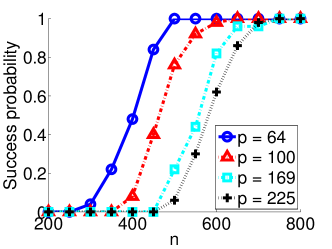
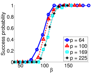
(a) Exponential Grid Structure

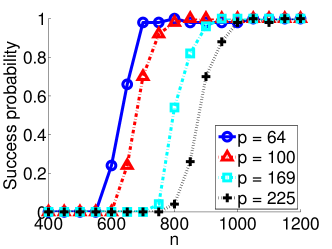
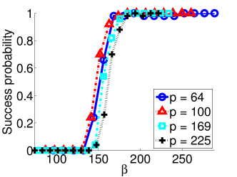
(b) Poisson Grid Structure

Figure 1: Probabilities of successful support recovery for the (a) exponential MRF, grid structure with parameters $\theta^{*}_{r}=0.1$ and $\theta^{*}_{rt}=1$, and the (b) Poisson MRF, grid structure with parameters $\theta^{*}_{r}=2$ and $\theta^{*}_{rt}=-0.1$. The empirical probability of successful edge recovery over 50 replicates is shown versus the sample size $n$ (left), and verses the re-scaled sample size $\beta=n/(\log p)$ (right). The empirical curves align for the latter, thus verifying the logarithmic dependence of $n$ on $p$ as obtained in our sparsistency analysis.

4.1 Simulation Studies

We provide a small simulation study that corroborates our sparsistency results; specifically Corollary 6 for the exponential graphical model, where node-conditional distributions follow an exponential distribution, and Corollary 7 for the Poisson graphical model, where node-conditional distributions follow a Poisson distribution. We instantiated the corresponding exponential and Poisson graphical model distributions in (15) and (14) for 4 nearest neighbor lattice graphs ($d=4$), with varying number of nodes, $p\in\{64,100,169,225\}$, and with identical edge weights for all edges: for exponential MRF, $\theta^{*}_{r}=0.1$ and $\theta^{*}_{rt}=1$, and, for Poisson MRF, $\theta^{*}_{r}=2$ and $\theta^{*}_{rt}=-0.1$. We generated i.i.d. samples from these distributions using Gibbs sampling, and solved our sparsity-constrained $M$-estimation problem by setting $\lambda_{n}=c\sqrt{\frac{\log p}{n}}$, following our corollaries; $c=3$ for exponential MRF, and 15 for Poisson MRF. We repeated each simulation 50 times and measured the empirical probability over the 50 trials that our penalized graph estimate in (17) successfully recovered all edges, that is, $P(\hat{E}=E^{*})$. The left panels of Figure 1(a) and Figure 1(b) show the empirical probability of successful edge recovery. In the right panel, we plot the empirical probability against a re-scaled sample size $\beta=n/(\log p)$. According to our corollaries, the sample size $n$ required for successful graph structure recovery scales logarithmically with the number of nodes $p$. Thus, we would expect the empirical curves for different problem sizes to more closely align with this re-scaled sample size on the horizontal axis, a result clearly seen in the right panels of Figure 1. This small numerical study thus corroborates our theoretical sparsistency results.

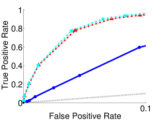
(a) Exponential Grid Structure

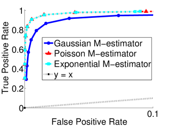
(b) Poisson Grid Structure

Figure 2: Receiver-operator curves (ROC) computed by varying the regularization parameter, $\lambda_{n}$. High-dimensional data is generated according to (a) the Exponential MRF with $(n,p)=(150,225)$ and to (b) the Poisson MRF with $(n,p)=(100,225)$. Results are compared for three $M$-estimators: that of the Poisson, exponential, and Gaussian distributions.

We also evaluate the comparative performance of our $M$-estimators for recovering the true edge structure from the different types of data. Specifically, we consider the three typical examples in our unified neighborhood selection approach: the Poisson $M$-estimator, the Exponential $M$-estimator, and the well-known Gaussian $M$-estimator by (Meinshausen and Bühlmann, 2006). In order to extensively compare their performances, we compute the receiver-operator-curves for the overall graph recovery by varying the regularization parameter, $\lambda_{n}$. In Figure 2, the same graph structures for the exponential MRF ($\theta^{*}_{r}=0.1$ and $\theta^{*}_{rt}=1$) and the Poisson MRF ($\theta^{*}_{r}=2$ and $\theta^{*}_{rt}=-0.1$) with 4 nearest neighbors, are used as in the previous simulation. Moreover, we focus on the high-dimensional regime where $n<p$. As shown in the figure, exponential and Poisson $M$-estimators outperform and have significant advantage over Gaussian neighborhood selection approach if the data is generated according to exponential or Poisson MRFs. One interesting phenomenon we observe is that exponential and Poisson $M$-estimators perform similarly regardless of the underlying graphical model distribution. This likely occurs as our estimator maximizes the conditional likelihoods by fitting penalized GLMs. Note that GLMs assume that the conditional mean of the regression model follows an exponential family distribution. As both the Poisson distribution and the exponential distribution have the same mean, the rate parameter, $\lambda$, we would expect GLM-based methods that fit conditional means to perform similarly.

As discussed at end of Section 2, the exponential and Poisson graphical models are able to capture only negative conditional dependencies between random variables, and our corresponding $M$-estimators are computed under this constraint. In our last simulation, we evaluate the impact of this restriction when the true graph contains both positive and negative edge weights. As there does not exist a proper MRF related to the Poisson and exponential distributions with both positive and negative dependencies, we resort to generating data from via a copula transform. In particular, we first generate multivariate Gaussian samples from $N(0,\Sigma$) where $\Theta=\Sigma^{-1}$ is the precision matrix corresponding to the 4 nearest neighbor grid structure previously considered. Specifically, $\Theta$ has all ones on the diagonal and $\theta_{rt}^{*}=\pm 0.2$ with equal probabilities. We then use a standard copula transform to make the marginals of the generated data approximately Poisson. Figure 3 again present receiver operator curves (ROC) for the three different classes of $M$-estimators on the copula transformed data, transformed to the Poisson distribution. In the left of Figure 3, we consider signed support recovery where we define the true positive rate as $\displaystyle\frac{\text{$\#$ of edges s.t. $\text{sign}(\theta_{rt}^{*})=\text{sign}(\widehat{\theta}_{rt})$ }}{\text{$\#$ of edges}}$. In the right, on the other hand, we ignore the positive edges so that true positive rate is now $\displaystyle\frac{\text{$\#$ of edges s.t. $\text{sign}(\theta_{rt}^{*})=\text{sign}(\widehat{\theta}_{rt})=-1$ }}{\text{$\#$ of negative edges}}$. Note that the false positive rate is also defined similarly. As expected, the results indicate that our Poisson and exponential $M$-estimators fail to recover the edges with positive conditional dependencies recovered by the Gaussian $M$-estimator. However, when attention is restricted to negative conditional dependencies, our method outperforms the Gaussian $M$-estimator. Notice also that for the exponential and Poisson $M$-estimators, the highest false positive rate achieved is around $0.15$. This likely occurs due to the constraints enforced by our $M$-estimators that force the weights of potential positive conditional dependent edges to be zero. Thus, while the restrictions on the edge weights may be severe, for the purpose of estimating negative conditional dependencies with limited false positives, the Poisson and exponential $M$-estimators have an advantage.

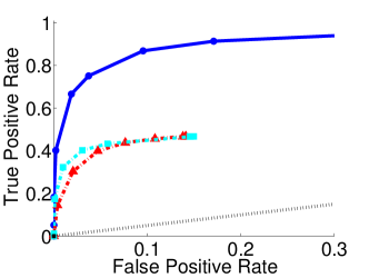
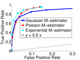
Figure 3: Receiver-operator curves (ROC) computed by varying the regularization parameter, $\lambda_{n}$, for data, $(n,p)=(200,225)$, generated via Poisson copula transform according to a network with both positive and negative conditional dependencies. Left plot denotes results on overall edge recovery, while right plot denotes recovery of the edges with negative weights corresponding to negative conditional dependencies.

4.2 Real Data Examples

To demonstrate the versatility of our family of graphical models, we also provide two real data examples: a meta-miRNA inhibitory network estimated by the Poisson graphical model, Figure 4, and a cell signaling network estimated by the exponential graphical model, Figure 5.

When applying our family of graphical models, there is always a question of whether our model is an appropriate fit for the observed data. Typically, one can assess model fit using goodness-of-fit tests. For the Gaussian graphical model, this reduces to testing whether the data follows a multivariate Gaussian distribution. For general exponential family graphical models, testing for goodness-of-fit is more challenging. Some have proposed likelihood ratio tests specifically for lattice systems with a fixed and known dependence structure (Besag, 1974). When the network structure is unknown, however, there are no such existing tests. While we leave the development of an exact test to future work, we provide a heuristic that can help us understand whether our model is appropriate for a given dataset.

Recall that our model assumes that conditional on its node-neighbors, each variable is distributed according to an exponential family. Thus, if the neighborhood is known, our conditional models are simply GLMs, for which the goodness-of-fit can be assessed compared to a null model by a likelihood ratio test (McCullagh and Nelder, 1989). When neighborhoods must be estimated, and specifically when estimated via an $\ell_{1}$-norm penalty, the resulting ratio of likelihoods no longer follow a chi-squared distribution (Bühlmann, 2011). Recently, for the $\ell_{1}$ linear regression case, Lockhart et al. (2014) have shown that the difference in the residual sums of squares follows an exponential distribution. Similar results have not yet been extended to the penalized GLM case. In the absence of such tests, we propose a simple heuristic: for each node, first estimate the node-neighborhood via our proposed M-estimator. Next, assuming the neighborhood is fixed, fit a GLM and compare the fit of this model to that of a null model (only an intercept term) via the likelihood ratio test. One can then heuristically assess the overall goodness-of-fit by examining the fit of a GLM to all the nodes. This procedure is clearly not an exact test, and following from Lockhart et al. (2014), it is likely conservative. In the absence of an exact test, which we leave for future work, this heuristic provides some assurances about the appropriateness of our model for real data.

4.2.1 Poisson Graphical Model: Meta-miRNA Inhibitory Network

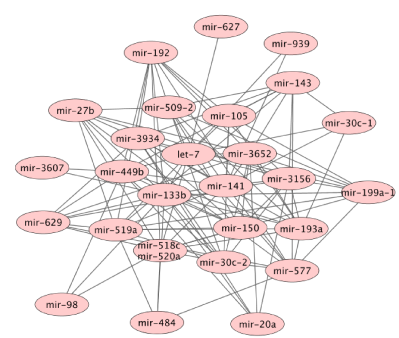
Figure 4: Meta-miRNA inhibitory network for breast cancer estimated via Poisson graphical models from miRNA-sequencing data. Level III data from TCGA was processed into tightly correlated clusters, meta-miRNAs, with the driver miRNAs identified for each cluster taken as the set of nodes for our network. The Poisson network reveals major inhibitory relationships between three hub miRNAs, two of which have been previously identified as tumor suppressors in breast cancer.

Gaussian graphical models have often been used to study high-throughput genomic networks estimated from microarray data (Pe’er et al., 2001; Friedman, 2004; Wei and Li, 2007). Many high-throughput technologies, however, do not produce even approximately Gaussian data, so that our class of graphical models could be particularly important for estimating genomic networks from such data. We demonstrate the applicability of our class of models by estimating a meta-miRNA inhibitory network for breast cancer estimated by a Poisson graphical model. Level III breast cancer miRNA expression (Cancer Genome Atlas Research Network, 2012) as measured by next generation sequencing was downloaded from the TCGA portal (http://tcga-data.nci.nih.gov/tcga/). MicroRNAs (miRNA) are short RNA fragments that are thought to be post-transcriptional regulators, predominantly inhibiting translation. Measuring miRNA expression by high-throughput sequencing results in count data that is zero-inflated, highly skewed, and whose total count volume depends on experimental conditions (Li et al., 2011). Data was processed to be approximately Poisson by following the steps described in (Allen and Liu, 2013). In brief, the data was quantile corrected to adjust for sequencing depth (Bullard et al., 2010); the miRNAs with little variation across the samples, the bottom 50%, were filtered out; and the data was adjusted for possible over-dispersion using a power transform and a goodness of fit test (Li et al., 2011). We also tested for batch effects in the resulting data matrix consisting of 544 subjects and 262 miRNAs: we fit a Poisson ANOVA model (Leek et al., 2010), and only found 4% of miRNAs to be associated with batch labels; and thus no significant batch association was detected. As several miRNAs likely target the same gene or genes in the same pathway, we expect there to be strong positive dependencies among variables that cannot be captured directly by our Poisson graphical model which only permits negative conditional relationships. Thus, we will use our model to study inhibitory relationships between what we term meta-miRNAs, or groups of miRNAs that are tightly positively correlated. To accomplish this, we further processed our data to form clusters of positively correlated miRNAs using hierarchical clustering with average linkage and one minus the correlation as the distance metric. This resulted in 40 clusters of tightly positively correlated miRNAs. The nodes of our meta-miRNA network were then taken as a the medoid, or median centroid defined as the miRNA closest in Euclidean distance to the cluster centroid, in each group.

A Poisson graphical model was fit to the meta-miRNA data by performing neighborhood selection with the sparsity of the graph determined by stability selection (Liu et al., 2010). The heuristic previously discussed was used to assess goodness-of-fit for our model. Out of the 40 node-neighborhoods tested via a likelihood ratio test, 36 exhibited $p$-values less than 0.05, and 34 were less than 0.05/40, the Bonferroni-adjusted significance level. These results show that the Poisson GLM is a significantly better fit for the majority of node-neighborhoods than the null model, indicating that our Poisson graphical model is appropriate for this data. The results of our estimated Poisson graphical model, Figure 4 (left), are consistent with the cancer genomics literature. First, the meta-miRNA inhibitory network has three major hubs. Two of these, miR-519 and miR-520, are known to be breast cancer tumor suppressors, suppressing growth by reducing HuR levels (Abdelmohsen et al., 2010) and by targeting NF-KB and TGF-beta pathways (Keklikoglou et al., 2012) respectively. The third major hub, miR-3156, is a miRNA of unknown function; from its major role in our network, we hypothesize that miR-3156 is also associated with tumor suppression. Also interestingly, let-7, a well-known miRNA involved in tumor metastasis (Yu et al., 2007), plays a central role in our network, sharing edges with the five largest hubs. This suggests that our Poisson graphical model has recovered relevant negative relationships between miRNAs with the five major hubs acting as suppressors, and the central let-7 miRNA and those connected to each of the major hubs acting as enhancers of tumor progression in breast cancer.

4.2.2 Exponential Graphical Model: Inhibitory Cell-Signaling Network

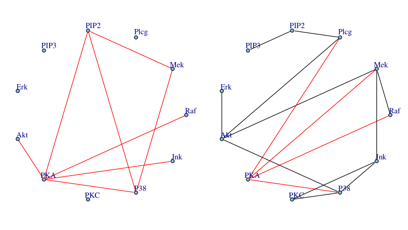
Figure 5: Cell signaling network estimated from flow cytometry data via exponential graphical models (left) and Gaussian graphical models (right). The exponential graphical model was fit to un-transformed flow cytometry data measuring 11 proteins, and the Gaussian graphical model to log-transformed data. Estimated negative conditional dependencies are given in red. Both networks identify PKA (protein kinase A) as a major inhibitor, consistent with previous results.

We demonstrate our exponential graphical model, derived from the univariate exponential distribution, using a protein signaling example (Sachs et al., 2005). Multi-florescent flow cytometry was used to measure the presence of eleven proteins ($p=11$) in $n=7462$ cells. This data set was first analyzed using Bayesian Networks in Sachs et al. (2005) and then using the graphical lasso algorithm in Friedman et al. (2007). Measurements from flow-cytometry data typically follow a left skewed distribution. Thus to model such data, these measurements are typically normalized to be approximately Gaussian using a log transform after shifting the data to be non-negative (Herzenberg et al., 2006). Here, we demonstrate the applicability of our exponential graphical models to recover networks directly from continuous skewed data, so that we learn the network directly from the flow-cytometry data without any log or such transforms. Our pre-processing is limited to shifting the data for each protein so that it consists of non-negative values. For comparison purposes, we also fit a Gaussian graphical model to the log-transformed data.

We then learned an exponential and Gaussian graphical model from this flow cytometry data using stability selection (Liu et al., 2010) to select the sparsity of the graphs. The goodness-of-fit heuristic previously described was used to assess the appropriateness of our model. Out of the eight connected node-neighborhoods, the likelihood ratio test was statistically significant for seven neighborhoods, indicating that our exponential GLM is a better fit than the null model. The estimated protein-signaling network is shown on the right in Figure 5 with that of the Gaussian graphical model fit to the log-transformed data on the left. Estimated negative conditional dependencies are shown in red. Recall that the exponential graphical model restricts the edge weights to be non-negative; because of the negative inverse link, this implies that only negative conditional associations can be estimated. Notice that our exponential graphical model finds that PKA, protein kinase A, is a major protein inhibitor in cell signaling networks. This is consistent with the inhibitory relationship of PKA as estimated by the Gaussian graphical model, right Figure 5, as well as its hub status in the Bayesian network of (Sachs et al., 2005). Interestingly, our exponential graphical model also finds a clique between PIP2, Mek, and P38, which was not found by Gaussian graphical models.

5 Discussion

We study what we call the class of exponential family graphical models that arise when we assume that node-wise conditional distributions follow exponential family distributions. Our work broadens the class of off-the-shelf graphical models from classical instances such as Ising and Gaussian graphical models. In particular, our class of graphical models provide closed form multivariate densities as extensions of several univariate exponential family distributions (e.g. Poisson, exponential, negative binomial) where few currently exist; and thus may be of further interest to the statistical community. Further, we provide simple M-estimators for estimating any of these graphical models from data, by fitting node-wise penalized conditional exponential family distributions, and show that these estimators enjoy strong statistical guarantees. The statistical analyses of our M-estimators required subtle techniques that may be of general interest in the analysis of sparse M-estimation.

There are many avenues of future work related to our proposed models. We assume that all conditional distributions are members of an exponential family. To determine whether this assumption is appropriate in practice for real data, a goodness-of-fit procedure is needed. While we have proposed a heuristic to this effect, more work is needed to determine a rigorous likelihood ratio test for testing model fit. For several instances of our proposed class of models, specifically those with variables with infinite domains, severe restrictions on the parameter space are sometimes needed. For instance, the Poisson and exponential graphical models studied in Section 4, could only model negative conditional dependencies, which may not always be desirable in practice. A key question for future work is whether these restrictions can be relaxed for particular exponential family distributions. Finally, while we have focused on single parameter exponential families, it would be interesting to investigate the consequences of using multi-parameter exponential family distributions. Overall, our work has opened avenues for learning Markov networks from a broad class of univariate distributions, the properties and applications of which leave much room for future research.

Acknowledgments

We would like to acknowledge support for this project from ARO W911NF-12-1-0390, NSF IIS-1149803, IIS-1320894, IIS-1447574, and DMS-1264033 (PR and EY); NSF DMS-1264058 and DMS-1209017 (GA); and the Houston Endowment and NSF DMS-1263932 (ZL).

A Proof of Theorem 2

The proof follows the development in Besag (1974), where they consider the case with $k=2$. We define $Q(X)$ as $Q(X):=\log(P(X)/P({\bf 0}))$, for any $X=(X_{1},\ldots,X_{p})\in\mathcal{X}^{p}$ where $P({\bf 0}))$ denotes the probability that all random variables take 0. Given any $X$, also denote $\overline{X}_{r:0}:=(X_{1},\ldots,X_{r-1},0,X_{r+1},\ldots,X_{p})$. Now, consider the following the most general form for $Q(X)$:

$$Q(X)=\sum_{1\leq r\leq p}X_{r}G_{r}(X_{r})+\ldots+\sum_{1\leq r_{1}<r_{2}<\ldots<r_{k}\leq p}X_{r_{1}}\ldots X_{r_{k}}G_{r_{1}\ldots r_{k}}(X_{r_{1}},\ldots,X_{r_{k}}),$$ (21)

since the joint distribution has factors of at most size $k$. By the definition of $Q$ and some algebra (See Section 2 of Besag (1974) for details), it can then be seen that

$$\exp(Q(X)-Q(\overline{X}_{r:0}))$$

$$=\ P(X_{r}|X_{1},\ldots,X_{r-1},X_{r+1},\ldots,X_{p})/P(0|X_{1},\ldots,X_{r-1},X_{r+1},\ldots,X_{p}).$$ (22)

Now, consider the simplifications of both sides of (A). For notational simplicity, we fix $r=1$ for a while. Given the form of $Q(X)$ in (21), we have

$$Q(X)-Q(\overline{X}_{1:0})=\ X_{1}\bigg{(}G_{1}(X_{1})+\sum_{2\leq t\leq p}X_{t}G_{1t}(X_{1},X_{t})+\ldots$$

$$+\sum_{2\leq t_{2}<t_{3}<\ldots<t_{k}\leq p}X_{t_{2}}\ldots X_{t_{k}}G_{1t_{2}\ldots t_{k}}(X_{1},X_{t_{2}}\ldots,X_{t_{k}})\bigg{)}.$$ (23)

By given the exponential family form of the node-conditional distribution specified in the statement, right-hand side of (A) become

$$\log\frac{P(X_{1}|X_{2},\ldots,X_{p})}{P(0|X_{2},\ldots,X_{p})}=E(X_{V\backslash 1})(B(X_{1})-B(0))+(C(X_{1})-C(0)).$$ (24)

Setting $X_{t}=0$ for all $t\neq 1$ in (A) and (24), we obtain,

$$X_{1}G_{1}(X_{1})=E({\bf 0})(B(X_{1})-B(0))+(C(X_{1})-C(0)).$$

Setting $X_{t_{2}}=0$ for all $t_{2}\not\in\{1,t\}$,

$$X_{1}G_{1}(X_{1})+X_{1}X_{t}G_{1t}(X_{1},X_{t})=E(0,\ldots,X_{t},\ldots,0)(B(X_{1})-B(0))+(C(X_{1})-C(0)).$$

Recovering the index 1 back to $r$ yields

$$X_{r}G_{r}(X_{r})=E({\bf 0})(B(X_{r})-B(0))+(C(X_{r})-C(0)),$$

$$X_{r}G_{r}(X_{r})+X_{r}X_{t}G_{rt}(X_{r},X_{t})=E(0,\ldots,X_{t},\ldots,0)(B(X_{r})-B(0))+(C(X_{r})-C(0)).$$

Similarly,

$$X_{t}G_{t}(X_{t})+X_{r}X_{t}G_{rt}(X_{r},X_{t})=E(0,\ldots,X_{r},\ldots,0)(B(X_{t})-B(0))+(C(X_{t})-C(0)).$$ (25)

From the above three equations, we obtain:

$$X_{r}X_{t}G_{rt}(X_{r},X_{t})=\theta_{rt}(B(X_{r})-B(0))(B(X_{t})-B(0)).$$

More generally, by considering non-zero triplets, and setting $X_{v}=0$ for all $v\not\in\{r,t,u\}$, we obtain,

$$X_{r}G_{r}(X_{r})+X_{r}X_{t}G_{rt}(X_{r},X_{t})+X_{r}X_{u}G_{ru}(X_{r},X_{u})+X_{r}X_{t}X_{u}G_{rtu}(X_{r},X_{t},X_{u})=$$

$$E(0,\ldots,X_{t},\ldots,X_{u},\ldots,0)(B(X_{r})-B(0))+(C(X_{r})-C(0)),$$ (26)

so that by a similar reasoning we can obtain

$$X_{r}X_{t}X_{u}G_{rtu}(X_{r},X_{t},X_{u})=\theta_{rtu}(B(X_{r})-B(0))(B(X_{t})-B(0))(B(X_{u})-B(0)).$$

More generally, we can show that

$$X_{t_{1}}\ldots X_{t_{k}}G_{t_{1},\ldots,t_{k}}(X_{t_{1}},\ldots,X_{t_{k}})=\theta_{t_{1},\ldots,t_{k}}(B(X_{t_{1}})-B(0))\ldots(B(X_{t_{k}})-B(0)).$$

Thus, the $k$-th order factors in the joint distribution as specified in (21) are tensor products of $(B(X_{r})-B(0))$, thus proving the statement of the theorem.

B Proof of Proposition 3

By the definition of (20) with the following simple calculation, the moment generating function of $X_{r}^{2}$ becomes:

$$\log\mathbb{E}[\exp(aX_{r}^{2})] =\log\int_{X}\exp\Big{\{}aX_{r}^{2}+\sum_{t\in V}\theta_{t}^{*}X_{t}+\sum_{(t,u)\in E}\theta_{tu}^{*}\,X_{t}\,X_{u}+\sum_{t\in V}C(X_{t})-A(\theta^{*})\Big{\}}$$

$$=\bar{A}_{r}(a;\theta^{*})-\bar{A}_{r}(0;\theta^{*}).$$

Suppose that $a\leq 1$. Then, by a Taylor Series expansion, we have for some $\nu\in[0,1]$,

$$\bar{A}_{r}(a;\theta^{*})-\bar{A}_{r}(0;\theta^{*}) =a\frac{\partial}{\partial\eta}\bar{A}_{r}(0;\theta^{*})+\frac{1}{2}a^{2}\frac{\partial^{2}}{\partial\eta^{2}}\bar{A}_{r}(\nu a;\theta^{*})\leq\kappa_{v}a+\frac{1}{2}\kappa_{h}a^{2},$$

where the inequality uses Condition (C3). Note that since the derivative of log-partition function is the mean of the corresponding sufficient statistics and $\bar{A}_{r}(0;\theta)=A(\theta)$, $\frac{\partial}{\partial\eta}\bar{A}_{r}(0;\theta^{*})=\mathbb{E}[X_{r}^{2}]\leq\kappa_{v}$ by assumption. Thus, by the standard Chernoff bounding technique, for all positive $a\leq 1$,

$$P\bigg{(}\frac{1}{n}\sum_{i=1}^{n}\big{(}X_{r}^{(i)}\big{)}^{2}\geq\delta\bigg{)} \leq\exp(-n\delta a+n\kappa_{v}a+\frac{n}{2}\kappa_{h}a^{2})$$

With the choice of $a=\frac{\delta-\kappa_{v}}{\kappa_{h}}\leq 1$, we obtain

$$P\bigg{(}\frac{1}{n}\sum_{i=1}^{n}\big{(}X_{r}^{(i)}\big{)}^{2}\geq\delta\bigg{)}\leq\exp\bigg{(}-n\frac{(\delta-\kappa_{v})^{2}}{2\kappa_{h}}\bigg{)}\leq\exp\Big{(}-n\frac{\delta^{2}}{8\kappa_{h}}\Big{)}$$

provided that $\delta\leq 2\kappa_{v}/3$, as in the statement.

C Proof of Proposition 4

Let $\bar{v}\in\mathbb{R}^{p+\binom{p}{2}}$ be the zero-padded parameter with only one non-zero coordinate, which is $1$, for the sufficient statistics $X_{r}$ so that $\|\bar{v}\|_{2}=1$. A simple calculation shows that

$$\log\mathbb{E}[\exp(X_{r})]=A(\theta^{*}+\bar{v})-A(\theta^{*}).$$

By a Taylor Series expansion and Condition (C3), we have for some $\nu\in[0,1]$,

$$A(\theta^{*}+\bar{v})-A(\theta^{*}) =\nabla A(\theta^{*})\cdot\bar{v}+\frac{1}{2}\bar{v}^{T}\nabla^{2}A(\theta^{*}+\nu\bar{v})\bar{v}$$

$$\overset{(i)}{\leq}\mathbb{E}[X_{r}]\|\bar{v}\|_{2}+\frac{1}{2}\frac{\partial^{2}}{\partial\theta_{r}^{2}}A(\theta^{*}+\nu\bar{v})\|\bar{v}\|_{2}^{2}\leq\kappa_{m}+\frac{1}{2}\kappa_{h},$$

where the inequality $(i)$ uses the fact that $\bar{v}$ has only nonzero element for the sufficient statistics $X_{r}$. Thus, again by the standard Chernoff bounding technique, for any positive constant $a$, $P\left(X_{r}\geq a\right)\leq\exp(-a+\kappa_{m}+\frac{1}{2}\kappa_{h})$, and by setting $a=\delta\log\eta$ we have

$$P\left(X_{r}\geq\delta\log\eta\right) \leq\exp(-\delta\log\eta+\kappa_{m}+\frac{1}{2}\kappa_{h})\leq c\eta^{-\delta},$$

where $c=\exp(\kappa_{m}+\frac{1}{2}\kappa_{h})$, as claimed.

D Proof of Theorem 5

In this section, we sketch the proof of Theorem 5 following the primal-dual witness proof technique in Wainwright (2009); Ravikumar et al. (2010). We first note that the optimality condition of the convex program (19) can be written as

$$\nabla\ell(\widehat{\theta};X^{1:n})+\lambda_{n}\widehat{Z}=0,$$ (27)

where $\widehat{Z}$ is a length $p$ vector: $\widehat{Z}_{\backslash r}\in\partial\|\widehat{\theta}_{\backslash r}\|_{1}$ is a length $(p-1)$ subgradient vector where $\widehat{Z}_{rt}=$ sign$(\widehat{\theta}_{rt})$ if $\widehat{\theta}_{rt}\neq 0$, and $|\widehat{Z}_{rt}|\leq 1$ otherwise; while $\widehat{Z}_{r}$, corresponding to $\theta_{r}$, is set to 0 since the nodewise term $\theta_{r}$ is not penalized in the $M$-estimation problem (19).

Note that in a high-dimensional regime with $p\gg n$, the convex program (19) is not necessarily strictly convex, so that it might have multiple optimal solutions. However, the following lemma, adapted from Ravikumar et al. (2010), shows that nonetheless the solutions share their support set under certain conditions. We first recall the notation $S=\{(r,t):t\in N^{*}(r)\}$ to denote the true neighborhood of node $r$, and $S^{c}$ to denote its complement.

Lemma 8

Suppose that there exists a primal optimal solution $\widehat{\theta}$ with associated subgradient $\widehat{Z}$ such that $\|\widehat{Z}_{S^{c}}\|_{\infty}<1$. Then, any optimal solution $\tilde{\theta}$ will satisfy $\tilde{\theta}_{S^{c}}=0$. Moreover, under the condition of $\|\widehat{Z}_{S^{c}}\|_{\infty}<1$, if $Q_{SS}^{*}$ is invertible, then $\widehat{\theta}$ is the unique optimal solution of (19).

Proof  This lemma can be proved by the same reasoning developed for the special cases Wainwright (2009); Ravikumar et al. (2010) in our framework; As in the previous works, for any node-conditional distribution in the form of exponential family, we are solving the convex objective with $\ell_{1}$ regularizer (19). Therefore, the problem can be written as an equivalent constrained optimization problem, and by the complementary slackness, for any optimal solution $\tilde{\theta}$, we have $\langle\widehat{Z},\tilde{\theta}\rangle=\|\tilde{\theta}\|_{1}$. This simply implies that for all index $j$ for which $|\widehat{Z}_{j}|<1$, $\tilde{\theta}_{j}=0$ (See Ravikumar et al. (2010) for details). Therefore, if there exists a primal optimal solution $\widehat{\theta}$ with associated subgradient $\widehat{Z}$ such that $\|\widehat{Z}_{S^{c}}\|_{\infty}<1$, then, any optimal solution $\tilde{\theta}$ will satisfy $\tilde{\theta}_{S^{c}}=0$ as claimed.

Finally, we consider the restricted optimization problem subject to the constraint $\theta_{S^{C}}=0$. For this restricted optimization problem, if the Hessian, $Q_{SS}^{*}$, is positive definite as assumed in the lemma, then, this restricted problem is strictly convex, and its solution is unique. Moreover, since all primal optimal solutions of (19), $\tilde{\theta}$, satisfy $\tilde{\theta}_{S^{c}}=0$ as discussed, the solution of the restricted problem is the unique solution of (19).  

We use this lemma to prove the theorem following the primal-dual witness proof technique in Wainwright (2009); Ravikumar et al. (2010). Specifically, we explicitly construct a pair $(\widehat{\theta},\widehat{Z})$ as follows (denoting the true support set of the edge parameters by $S$):

1. Recall that $\theta(r)=(\theta_{r},\theta_{\backslash r})\in\mathbb{R}\times\mathbb{R}^{p-1}$. We first fix $\theta_{S^{c}}=0$ and solve the restricted optimization problem: $(\widehat{\theta}_{r},\,\widehat{\theta}_{S},0)=\operatorname*{arg\,min}_{\theta_{r}\in\mathbb{R},\,(\theta_{S},0)\in\mathbb{R}^{p-1}}\{\ell(\theta;X^{1:n})+\lambda_{n}\|\theta_{S}\|_{1}\}$, and $\widehat{Z}_{S}=$ sign$(\widehat{\theta}_{S})$.

2. We set $\widehat{\theta}_{S^{c}}=0$.

3. We set $\widehat{Z}_{S^{c}}$ to satisfy the condition (27) with $\widehat{\theta}$ and $\widehat{Z}_{S}$.

By construction, the support of $\widehat{\theta}$ is included in the true support $S$ of $\theta^{*}$, so that we would finish the proof of the theorem provided (a) $\widehat{\theta}$ satisfies the stationary condition of  (19), as well as the condition $\|\widehat{Z}_{S^{c}}\|_{\infty}<1$ in Lemma 8 with high probability, so that by Lemma 8, the primal solution $\widehat{\theta}$ is guaranteed to be unique; and (b) the support of $\widehat{\theta}$ is not strictly within the true support $S$. We term these conditions strict dual feasibility, and sign consistency respectively.

We will now rewrite the subgradient optimality condition (27) as

$$\nabla^{2}\ell(\theta^{*};X^{1:n})(\widehat{\theta}-\theta^{*})=-\lambda_{n}\widehat{Z}+W^{n}+R^{n},$$

where $W^{n}:=-\nabla\ell(\theta^{*};X^{1:n})$ is the sample score function (that we will show is small with high probability), and $R^{n}$ is the remainder term after coordinate-wise applications of the mean value theorem; $R_{j}^{n}=[\nabla^{2}\ell(\theta^{*};X^{1:n})-\nabla^{2}\ell(\bar{\theta}^{(j)};X^{1:n})]_{j}^{T}(\widehat{\theta}-\theta^{*})$, for some $\bar{\theta}^{(j)}$ on the line between $\widehat{\theta}$ and $\theta^{*}$, and with $[\cdot]_{j}^{T}$ being the $j$-th row of a matrix.

Recalling the notation for the Fisher information matrix $Q^{*}:=\nabla^{2}\ell(\theta^{*};X^{1:n})$, we then have

$$Q^{*}(\widehat{\theta}-\theta^{*})=-\lambda_{n}\widehat{Z}+W^{n}+R^{n}.$$

From now on, we provide lemmas that respectively control various terms in the above expression: the score term $W^{n}$, the deviation $\widehat{\theta}-\theta^{*}$, and the remainder term $R^{n}$. The first lemma controls the score term $W^{n}$:

Lemma 9

Suppose that we set $\lambda_{n}$ to satisfy $\frac{8(2-\alpha)}{\alpha}\sqrt{\kappa_{1}(n,p)\kappa_{4}}\sqrt{\frac{\log p}{n}}\leq\lambda_{n}\leq\frac{4(2-\alpha)}{\alpha}\allowbreak\kappa_{1}(n,p)\kappa_{2}(n,p)\kappa_{4}$ for some constant $\kappa_{4}\leq\min\{2\kappa_{v}/3,2\kappa_{h}+\kappa_{v}\}$. Suppose also that $n\geq\frac{8\kappa_{h}^{2}}{\kappa_{4}^{2}}\log p$. Then, given a incoherence parameter $\alpha\in(0,1]$,

$$P\left(\frac{2-\alpha}{\lambda_{n}}\|W^{n}\|_{\infty}\leq\frac{\alpha}{4}\right)\geq 1-c_{1}p^{\prime-2}-\exp(-c_{2}n)-\exp(-c_{3}n)$$

where $p^{\prime}:=\max\{n,p\}$.

The next lemma controls the deviation $\widehat{\theta}-\theta^{*}$:

Lemma 10

Suppose that $\lambda_{n}d\leq\frac{\rho_{\min}^{2}}{40\rho_{\max}\kappa_{3}(n,p)\log p^{\prime}}$ and $\|W^{n}\|_{\infty}\leq\frac{\lambda_{n}}{4}$. Then, we have

$$P\left(\|\widehat{\theta}_{S}-\theta_{S}^{*}\|_{2}\leq\frac{5}{\rho_{\min}}\sqrt{d}\lambda_{n}\right)\geq 1-c_{1}p^{\prime-2},$$ (28)

for some constant $c_{1}>0$.

The last lemma controls the Taylor series remainder term $R^{n}$:

Lemma 11

If $\lambda_{n}d\leq\frac{\rho_{\min}^{2}}{400\rho_{\max}\kappa_{3}(n,p)\log p^{\prime}}\frac{\alpha}{2-\alpha}$, and $\|W^{n}\|_{\infty}\leq\frac{\lambda_{n}}{4}$, then we have

$$P\left(\frac{\|R^{n}\|_{\infty}}{\lambda_{n}}\leq\frac{\alpha}{4(2-\alpha)}\right)\geq 1-c_{1}p^{\prime-2},$$ (29)

for some constant $c_{1}>0$.

The proof then follows from Lemmas 9, 10 and 11 in a straightforward fashion, following Ravikumar et al. (2010). Consider the choice of regularization parameter $\lambda_{n}=\frac{8(2-\alpha)}{\alpha}\sqrt{\kappa_{1}(n,p)\kappa_{4}}\sqrt{\frac{\log p}{n}}$. For a sample size greater $n\geq\max\{\frac{4}{\kappa_{1}(n,p)\kappa_{2}(n,p)^{2}\kappa_{4}},\frac{8\kappa_{h}^{2}}{\kappa_{4}^{2}}\}\allowbreak\log p$, the conditions of Lemma 9 are satisfied, so that we may conclude that $\|W^{n}\|_{\infty}\leq\frac{\alpha}{1-\alpha}\frac{\lambda_{n}}{4}\leq\frac{\lambda_{n}}{4}$ with high probability. Moreover, with a sufficiently large sample size such that $n\geq L^{\prime}\left(\frac{2-\alpha}{\alpha}\right)^{4}d^{2}\kappa_{1}(n,p)\kappa_{3}(n,p)^{2}\log p(\log p^{\prime})^{2}$ for some constant $L^{\prime}>0$ depending only on $\rho_{\min}$, $\rho_{\max}$, $\kappa_{4}$ and $\alpha$, it can be shown that the remaining condition of Lemma 11 (and hence the milder condition in Lemma 10) in turn is satisfied. Therefore, the resulting statements (28) and (29) of Lemmas 10 and 11 hold with high probability.

Strict dual feasibility. Following Ravikumar et al. (2010), we obtain

$$\|\widehat{Z}_{S^{c}}\|_{\infty}\ \leq\ |\!|\!|Q^{*}_{S^{c}S}(Q^{*}_{SS})^{-1}|\!|\!|_{\infty}\Big{[}\frac{\|W_{S}^{n}\|_{\infty}}{\lambda_{n}}+\frac{\|R_{S}^{n}\|_{\infty}}{\lambda_{n}}+1\Big{]}+\frac{\|W_{S^{c}}^{n}\|_{\infty}}{\lambda_{n}}+\frac{\|R_{S^{c}}^{n}\|_{\infty}}{\lambda_{n}}$$

$$\leq(1-\alpha)+(2-\alpha)\Big{[}\frac{\|W^{n}\|_{\infty}}{\lambda_{n}}+\frac{\|R^{n}\|_{\infty}}{\lambda_{n}}\Big{]}\leq(1-\alpha)+\frac{\alpha}{4}+\frac{\alpha}{4}=1-\frac{\alpha}{2}<1.$$

Correct sign recovery. To guarantee that the support of $\widehat{\theta}$ is not strictly within the true support $S$, it suffices to show that $\|\widehat{\theta}_{S}-\theta_{S}^{*}\|_{\infty}\leq\frac{\theta_{\min}^{*}}{2}$. From Lemma 10, we have $\|\widehat{\theta}_{S}-\theta_{S}^{*}\|_{\infty}\leq\|\widehat{\theta}_{S}-\theta_{S}^{*}\|_{2}\leq\frac{5}{\rho_{\min}}\sqrt{d}\lambda_{n}\leq\frac{\theta_{\min}^{*}}{2}$ as long as $\theta_{\min}^{*}\geq\frac{10}{\rho_{\min}}\sqrt{d}\lambda_{n}$. This completes the proof.

D.1 Proof of Lemma 9

For a fixed $t\in V\backslash r$, we define $V^{(i)}_{t}$ for notational convenience so that

$$W^{n}_{t}=\frac{1}{n}\sum_{i=1}^{n}X_{r}^{(i)}X_{t}^{(i)}-X_{t}^{(i)}D^{\prime}(\theta^{*}_{r}+\langle\theta^{*}_{\backslash r},X_{V\setminus r}^{(i)}\rangle)=\frac{1}{n}\sum_{i=1}^{n}V^{(i)}_{t}$$

Consider the upper bound on the moment generating function of $V^{(i)}_{t}$, conditioned on $X_{V\setminus r}^{(i)}$,

$$\ \mathbb{E}[\exp(aV_{t})|X_{V\setminus r}^{(i)}]=\int_{X_{r}}\exp\bigg{\{}a\big{[}X_{r}X_{t}^{(i)}-X_{t}^{(i)}D^{\prime}\big{(}\theta^{*}_{r}+\langle\theta^{*}_{\backslash r},X_{V\setminus r}^{(i)}\rangle\big{)}\big{]}$$

$$\ +\Big{(}X_{r}\big{(}\theta^{*}_{r}+\langle\theta^{*}_{\backslash r},X_{V\setminus r}^{(i)}\rangle\big{)}+C(X_{r})-D\big{(}\theta^{*}_{r}+\langle\theta^{*}_{\backslash r},X_{V\setminus r}^{(i)}\rangle\big{)}\Big{)}\bigg{\}}$$

$$= \ \exp\Big{\{}D\big{(}\theta^{*}_{r}+\langle\theta^{*}_{\backslash r},X_{V\setminus r}^{(i)}\rangle+aX_{t}^{(i)}\big{)}-D\big{(}\theta^{*}_{r}+\langle\theta^{*}_{\backslash r},X_{V\setminus r}^{(i)}\rangle\big{)}-aX_{t}^{(i)}D^{\prime}\big{(}\theta^{*}_{r}+\langle\theta^{*}_{\backslash r},X_{V\setminus r}^{(i)}\rangle\big{)}\Big{\}}$$

$$= \ \exp\Big{\{}\frac{a^{2}}{2}\big{(}{X_{t}^{(i)}}\big{)}^{2}D^{\prime\prime}\big{(}\theta^{*}_{r}+\langle\theta^{*}_{\backslash r},X_{V\setminus r}^{(i)}\rangle+\nu_{i}aX_{t}^{(i)}\big{)}\Big{\}}\quad\textrm{for some $\nu_{i}\in[0,1]$}$$

where the last equality holds by the second-order Taylor series expansion. Consequently, we have

$$\ \frac{1}{n}\sum_{i=1}^{n}\log\mathbb{E}[\exp(aV^{(i)}_{t})|X_{V\setminus r}^{(i)}]\leq\frac{1}{n}\sum_{i=1}^{n}\frac{a}{2}\big{(}X_{t}^{(i)}\big{)}^{2}D^{\prime\prime}\big{(}\theta^{*}_{r}+\langle\theta^{*}_{\backslash r},X_{V\setminus r}^{(i)}\rangle+\nu_{i}aX_{t}^{(i)}\big{)}.$$

First, we define the event: $\xi_{1}:=\Big{\{}\max_{i,s}|X_{r}^{(i)}|\leq 4\log p^{\prime}\Big{\}}$. Then, by Proposition 4, we obtain $P[\xi_{1}^{c}]\leq c_{1}\,npp^{\prime-4}\leq c_{1}\,p^{\prime-2}$. Provided that $a\leq\kappa_{2}(n,p)$, we can use Condition (C4) to control the second-order derivative of log-partition function and we obtain

$$\ \frac{1}{n}\sum_{i=1}^{n}\log\mathbb{E}[\exp(aV^{(i)}_{t})|X_{V\setminus r}^{(i)}]\leq\frac{\kappa_{1}(n,p)a^{2}}{2}\frac{1}{n}\sum_{i=1}^{n}\big{(}X_{t}^{(i)}\big{)}^{2}\quad\textrm{for $a\leq\kappa_{2}(n,p)$}$$

with probability at least $1-c_{1}p^{\prime-2}$. Now, for each index $t$, the variables $\frac{1}{n}\sum_{i=1}^{n}\big{(}X_{t}^{(i)}\big{)}^{2}$ satisfy the tail bound in Proposition 3. Let us define the event ${\displaystyle\xi_{2}:=\Big{\{}\max_{t\in V}}\ \frac{1}{n}\sum_{i=1}^{n}\big{(}X_{t}^{(i)}\big{)}^{2}\allowbreak\leq\kappa_{4}\Big{\}}$ for some constant $\kappa_{4}\leq\min\{2\kappa_{v}/3,2\kappa_{h}+\kappa_{v}\}$. Then, we can establish the upper bound of probability $P[\xi_{2}^{c}]$ by a union bound,

$$P[\xi_{2}^{c}]\leq\exp(-\frac{\kappa_{4}^{2}}{4\kappa_{h}^{2}}n+\log p)\leq\exp(-c_{2}n)$$

as long as $n\geq\frac{8\kappa_{h}^{2}}{\kappa_{4}^{2}}\log p$. Therefore, conditioned on $\xi_{1},\xi_{2}$, the moment generating function is bounded as follows:

$$\ \frac{1}{n}\sum_{i=1}^{n}\log\mathbb{E}[\exp(aV^{(i)}_{t})|X_{V\setminus r}^{(i)},\xi_{1},\xi_{2}]\leq\frac{\kappa_{1}(n,p)\kappa_{4}\,a^{2}}{2}\quad\textrm{for $a\leq\kappa_{2}(n,p)$}.$$

The standard Chernoff bound technique implies that for any $\delta>0$,

$$\ P\Big{[}\big{|}\frac{1}{n}\sum_{i=1}^{n}V^{(i)}_{t}\big{|}>\delta\ |\ \xi_{1},\xi_{2}\Big{]}\leq 2\exp\left(n\Big{(}\frac{\kappa_{1}(n,p)\kappa_{4}\,a^{2}}{2}-a\delta\Big{)}\right)\quad\textrm{for $a\leq\kappa_{2}(n,p)$}.$$

Setting $a=\frac{\delta}{\kappa_{1}(n,p)\kappa_{4}}$ yields

$$\ P\Big{[}\big{|}\frac{1}{n}\sum_{i=1}^{n}V^{(i)}_{t}\big{|}>\delta\ |\ \xi_{1},\xi_{2}\Big{]}\leq 2\exp\left(-\frac{n\delta^{2}}{2\kappa_{1}(n,p)\kappa_{4}}\right)\quad\textrm{for $\delta\leq\kappa_{1}(n,p)\kappa_{2}(n,p)\kappa_{4}$}.$$

Suppose that $\frac{\alpha}{2-\alpha}\frac{\lambda_{n}}{4}\leq\kappa_{1}(n,p)\kappa_{2}(n,p)\kappa_{4}$ for large enough $n$; thus setting $\delta=\frac{\alpha}{2-\alpha}\frac{\lambda_{n}}{4}$:

$$\ P\Big{[}\big{|}\frac{1}{n}\sum_{i=1}^{n}V^{(i)}_{t}\big{|}>\frac{\alpha}{2-\alpha}\frac{\lambda_{n}}{4}\ |\ \xi_{1},\xi_{2}\Big{]}\leq 2\exp\left(-\frac{\alpha^{2}}{(2-\alpha)^{2}}\frac{n\lambda_{n}^{2}}{32\kappa_{1}(n,p)\kappa_{4}}\right),$$

and by a union bound, we obtain

$$\ P\Big{[}\|W^{n}\|_{\infty}>\frac{\alpha}{2-\alpha}\frac{\lambda_{n}}{4}\ |\ \xi_{1},\xi_{2}\Big{]}\leq 2\exp\left(-\frac{\alpha^{2}}{(2-\alpha)^{2}}\frac{n\lambda_{n}^{2}}{32\kappa_{1}(n,p)\kappa_{4}}+\log p\right).$$

Finally, provided that $\lambda_{n}\geq\frac{8(2-\alpha)}{\alpha}\sqrt{\kappa_{1}(n,p)\kappa_{4}}\sqrt{\frac{\log p}{n}}$, we obtain

$$\ P\Big{[}\|W^{n}\|_{\infty}>\frac{\alpha}{2-\alpha}\frac{\lambda_{n}}{4}\Big{]}\leq c_{1}p^{\prime-2}+\exp(-c_{2}n)+\exp(-c_{3}n),$$

where we use the fact that the probability of occurring event $\mathcal{A}$ is upper bounded by $P(\mathcal{A})\leq P(\xi_{1}^{c})+P(\xi_{2}^{c})+P(\mathcal{A}|\xi_{1},\xi_{2})$.

D.2 Proof of Lemma 10

In order to establish the error bound $\|\widehat{\theta}_{S}-\theta_{S}^{*}\|_{2}\leq B$ for some radius $B$, several works (e.g. Negahban et al. (2012); Ravikumar et al. (2010)) proved that it suffices to show $F(u_{S})>0$ for all $u_{S}:=\theta_{S}-\theta_{S}^{*}$ s.t. $\|u_{S}\|_{2}=B$ where

$$F(u_{S}):=\ell(\theta_{S}^{*}+u_{S};X^{1:n})-\ell(\theta_{S}^{*};X^{1:n})+\lambda_{n}(\|\theta_{S}^{*}+u_{S}\|_{1}-\|\theta_{S}^{*}\|_{1}).$$

Note that $F(0)=0$, and for $\hat{u}_{S}:=\widehat{\theta}_{S}-\theta_{S}^{*}$, $F(\hat{u}_{S})\leq 0$. From now on, we show that $F(u_{S})$ is strictly positive on the boundary of the ball with radius $B=M\lambda_{n}\sqrt{d}$ where $M>0$ is a parameter that we will choose later in this proof. Some algebra yields

$$F(u_{S})\geq(\lambda_{n}\sqrt{d})^{2}\Big{\{}-\frac{1}{4}M+q^{*}M^{2}-M\Big{\}}$$ (30)

where $q^{*}$ is the minimum eigenvalue of $\nabla^{2}\ell(\theta_{S}^{*}+vu_{S};X^{1:n})$ for some $v\in[0,1]$. Moreover,

$$q^{*} :=\Lambda_{\min}\big{(}\nabla^{2}\ell(\theta_{S}^{*}+vu_{S})\big{)}$$

$$\geq\min_{v\in[0,1]}\Lambda_{\min}\big{(}\nabla^{2}\ell(\theta_{S}^{*}+vu_{S})\big{)}$$

$$\geq\Lambda_{\min}\big{[}\frac{1}{n}\sum_{i=1}^{n}D^{\prime\prime}(\theta^{*}_{r}+\langle\theta_{S}^{*},X_{S}^{(i)}\rangle)X_{S}^{(i)}\big{(}X_{S}^{(i)}\big{)}^{T}\big{]}$$

$$\quad\quad-\max_{v\in[0,1]}|\!|\!|\frac{1}{n}\sum_{i=1}^{n}D^{\prime\prime\prime}\big{(}\theta^{*}_{r}+\langle\theta_{S}^{*},X_{S}^{(i)}\rangle\big{)}\big{(}u_{S}^{T}X_{S}^{(i)}\big{)}X_{S}^{(i)}\big{(}X_{S}^{(i)}\big{)}^{T}|\!|\!|_{2}$$

$$\geq\rho_{\min}-\max_{v\in[0,1]}\max_{y}\frac{1}{n}\sum_{i=1}^{n}|D^{\prime\prime\prime}\big{(}\theta^{*}_{r}+\langle\theta_{S}^{*},X_{S}^{(i)}\rangle\big{)}|\ |\langle u_{S},X_{S}^{(i)}\rangle|\ \big{(}\langle X_{S}^{(i)},y\rangle\big{)}^{2}$$

where $y\in\mathbb{R}^{d}$ s.t $\|y\|_{2}=1$. Similarly as in the previous proof, we consider the event $\xi_{1}$ with probability at least $1-c_{1}p^{\prime-2}$. Then, since all the elements in vector $X_{S}^{(i)}$ is smaller than $4\log p^{\prime}$, $|\langle u_{S},X_{S}^{(i)}\rangle|\leq 4\log p^{\prime}\sqrt{d}\|u_{S}\|_{2}=4\log p^{\prime}M\lambda_{n}d$ for all $i$. At the same time, by Condition (C4), $|D^{\prime\prime\prime}((\theta^{*}_{r}+vu_{S})+\langle\theta_{S}^{*}+vu_{S},X_{S}^{(i)}\rangle)|\leq\kappa_{3}(n,p)$. Note that $\theta_{S}^{*}+vu_{S}$ is a convex combination of $\theta^{*}_{S}$ and $\widehat{\theta}_{S}$, and as a result, we can directly apply the Condition (C4). Hence, conditioned on $\xi_{1}$, we have

$$q^{*} \geq\rho_{\min}-4\rho_{\max}M\lambda_{n}d\kappa_{3}(n,p)\log p^{\prime},$$

As a result, assuming that $\lambda_{n}\leq\frac{\rho_{\min}}{8\rho_{\max}Md\kappa_{3}(n,p)\log p^{\prime}}$, $q^{*}\geq\frac{\rho_{\min}}{2}$. Finally, from (30), we obtain

$$F(u_{S})\geq(\lambda_{n}\sqrt{d})^{2}\Big{\{}-\frac{1}{4}M+\frac{\rho_{\min}}{2}M^{2}-M\Big{\}},$$

which is strictly positive for $M=\frac{5}{\rho_{\min}}$. Therefore, if $\lambda_{n}d\leq\frac{\rho_{\min}}{8\rho_{\max}M\kappa_{3}(n,p)\log p^{\prime}}\leq\frac{\rho_{\min}^{2}}{40\rho_{\max}\kappa_{3}(n,p)\log p^{\prime}}$, then

$$\|\widehat{\theta}_{S}-\theta_{S}^{*}\|_{2}\leq\frac{5}{\rho_{\min}}\sqrt{d}\lambda_{n},$$

which completes the proof.

D.3 Proof of Lemma 11

In the proof, we are going to show that $\|R^{n}\|_{\infty}\leq 4\kappa_{3}(n,p)\log p^{\prime}\rho_{\max}\|\widehat{\theta}_{S}-\theta_{S}^{*}\|_{2}^{2}$. Then, since the conditions of Lemma 11 are stronger than those of Lemma 10, from the result of Lemma 10, we can conclude that

$$\|R^{n}\|_{\infty}\leq\frac{100\kappa_{3}(n,p)\rho_{\max}\log p^{\prime}}{\rho_{\min}^{2}}\lambda_{n}^{2}d,$$

as claimed in Lemma 11.

From the definition of $R^{n}$, for a fixed $t\in V\backslash r$, $R_{t}^{n}$ can be written as

$$\frac{1}{n}\sum_{i=1}^{n}\Big{[}D^{\prime\prime}\big{(}\theta^{*}_{r}+\langle\theta^{*}_{\backslash r},X_{V\setminus r}^{(i)}\rangle\big{)}-D^{\prime\prime}\big{(}\bar{\theta}_{s}+\langle\bar{\theta}^{(t)},X_{V\setminus r}^{(i)}\rangle\big{)}\Big{]}\Big{[}X_{V\setminus r}^{(i)}\big{(}X_{V\setminus r}^{(i)}\big{)}^{T}\Big{]}_{t}^{T}[\widehat{\theta}_{\backslash r}-\theta^{*}_{\backslash r}]$$

where $\bar{\theta}^{(t)}_{\backslash r}$ is some point in the line between $\widehat{\theta}_{\backslash r}$ and $\theta^{*}_{\backslash r}$, i.e., $\bar{\theta}^{(t)}_{\backslash r}=v_{t}\widehat{\theta}_{\backslash r}+(1-v_{t})\theta^{*}_{\backslash r}$ for $v_{t}\in[0,1]$. By another application of the mean value theorem, we have

$$R_{t}^{n}=-\frac{1}{n}\sum_{i=1}^{n}\left\{D^{\prime\prime\prime}\big{(}\bar{\bar{\theta}}_{s}+\langle\bar{\bar{\theta}}^{(t)}_{\backslash r},X_{V\setminus r}^{(i)}\rangle\big{)}X_{t}^{(i)}\right\}\left\{v_{t}[\widehat{\theta}_{\backslash r}-\theta^{*}_{\backslash r}]^{T}X_{V\setminus r}^{(i)}\big{(}X_{V\setminus r}^{(i)}\big{)}^{T}[\widehat{\theta}_{\backslash r}-\theta^{*}_{\backslash r}]\right\}$$

for a some point $\bar{\bar{\theta}}^{(t)}_{\backslash r}$ between $\bar{\theta}^{(t)}_{\backslash r}$ and $\theta^{*}_{\backslash r}$. Similarly in the previous proofs, conditioned on the event $\xi_{1}$, we obtain

$$|R_{t}^{n}|\leq\frac{4\kappa_{3}(n,p)\log p^{\prime}}{n}\sum_{i=1}^{n}\left\{v_{t}[\widehat{\theta}_{\backslash r}-\theta^{*}_{\backslash r}]^{T}X_{V\setminus r}^{(i)}\big{(}X_{V\setminus r}^{(i)}\big{)}^{T}[\widehat{\theta}_{\backslash r}-\theta^{*}_{\backslash r}]\right\}.$$

Performing some algebra yields

$$|R_{t}^{n}|\leq 4\kappa_{3}(n,p)\rho_{\max}\log p^{\prime}\,\|\widehat{\theta}_{S}-\theta_{S}^{*}\|_{2}^{2},\quad\textrm{for all $t\in V\backslash r$}$$

with probability at least $1-c_{1}p^{\prime-2}$, which completes the proof.

E Optimization Problems for Poisson and Exponential Graphical Model Neighborhood Selection

We propose to fit our family of graphical models by performing neighborhood selection, or maximizing the $\ell_{1}$-penalized log-likleihood for each node conditional on all other nodes. For several exponential families, however, further restrictions on the parameter space are needed to ensure a proper Markov Random Field. When performing neighborhood selection, these can be imposed by adding constraints to the penalized generalized linear models. We illustrate this by providing the optimization problems solved by our Poisson graphical model and exponential graphical model M-estimator that are used in Section 4.

Following from Section 3, the neighborhood selection problem for our family of models maximizes the likelihood of a node, $X_{r}$, conditional on all other nodes, $X_{V\backslash r}$. This conditional likelihood is regularized with an $\ell_{1}$ penalty to induce sparsity in the edge weights, $\theta(r)$ a $p-1$ dimensional vector, and constrained to enforce restrictions, $\theta(r)\in\mathcal{C}$, needed to yield a proper MRF:

$$\operatorname*{maximize}_{\theta(r)}\ \ \frac{1}{n}\sum_{i=1}^{n}\ell\left(X_{i,r}|X_{i,V\backslash r};\theta(r)\right)-\lambda_{n}\|\theta(r)\|_{1}\ \ \textrm{subject to}\ \ \theta(r)\in\mathcal{C},$$

where $\ell\left(X_{i,r}|X_{i,V\backslash r};\theta(r)\right)$ is the conditional log-likelihood for the exponential family. For the Poisson graphical model, the edge weights are constrained to be non-positive. This yields the following optimization problem:

$$\operatorname*{maximize}_{\theta(r)} \ \ \frac{1}{n}\sum_{i=1}^{n}\left[X_{r,i}X_{V\backslash r,i}^{T}\theta(r)-\mathrm{exp}\left(X_{V\backslash r,i}^{T}\theta(r)\right)\right]-\lambda_{n}\|\theta(r)\|_{1}$$

subject to $$\ \ \theta(r)\leq 0.$$

Similarly, the edge weights of the exponential graphical are restricted to be non-negative yielding:

$$\operatorname*{maximize}_{\theta(r)} \ \ \frac{1}{n}\sum_{i=1}^{n}\left[-X_{r,i}X_{V\backslash r,i}^{T}\theta(r)+\mathrm{log}\left(X_{V\backslash r,i}^{T}\theta(r)\right)\right]-\lambda_{n}\|\theta(r)\|_{1}$$

subject to $$\ \ \theta(r)\geq 0.$$

Note that we neglect the intercept term, assuming this to be zero as is common in other proposed neighborhood selection methods (Meinshausen and Bühlmann, 2006; Ravikumar et al., 2010; Jalali et al., 2011). Both of the neighborhood selection problems are concave problems with a smooth log-likelihood and linear constraints. While there are a plethora of optimization routines available to solve such problems, we have employed a projected gradient descent scheme which is guaranteed to converge to a global optimum (Daubechies et al., 2008; Beck and Teboulle, 2010).

References

- Abdelmohsen et al. (2010) K. Abdelmohsen, M. M. Kim, S. Srikantan, E. M. Mercken, S. E. Brennan, G. M. Wilson, R. de Cabo, and M. Gorospe. mir-519 suppresses tumor growth by reducing hur levels. Cell cycle, 9(7):1354–1359, 2010.
- Acemoglu (2009) D. Acemoglu. The crisis of 2008: Lessons for and from economics. Critical Review, 21(2-3):185–194, 2009.
- Allen and Liu (2013) G. I. Allen and Z. Liu. A local poisson graphical model for inferring networks from sequencing data. IEEE Trans. NanoBioscience, 12(1):1–10, 2013.
- Beck and Teboulle (2010) A. Beck and M. Teboulle. Gradient-based algorithms with applications to signal recovery problems. Convex Optimization in Signal Processing and Communications, pages 42–88, 2010.
- Besag (1974) J. Besag. Spatial interaction and the statistical analysis of lattice systems. Journal of the Royal Statistical Society. Series B (Methodological), 36(2):192–236, 1974.
- Bishop et al. (2007) Y. M. Bishop, S. E. Fienberg, and P. W. Holland. Discrete multivariate analysis. Springer Verlag, 2007.
- Bühlmann (2011) P. Bühlmann. Statistics for high-dimensional data. Springerverlag Berlin Heidelberg, 2011.
- Bullard et al. (2010) J. Bullard, E. Purdom, K. Hansen, and S. Dudoit. Evaluation of statistical methods for normalization and differential expression in mrna-seq experiments. BMC bioinformatics, 11(1):94, 2010.
- Cancer Genome Atlas Research Network (2012) Cancer Genome Atlas Research Network. Comprehensive molecular portraits of human breast tumours. Nature, 490(7418):61–70, 2012.
- Clifford (1990) P. Clifford. Markov random fields in statistics. In Disorder in physical systems. Oxford Science Publications, 1990.
- Daubechies et al. (2008) I. Daubechies, M. Fornasier, and I. Loris. Accelerated projected gradient method for linear inverse problems with sparsity constraints. Journal of Fourier Analysis and Applications, 14(5):764–792, 2008.
- Dobra and Lenkoski (2011) A. Dobra and A. Lenkoski. Copula gaussian graphical models and their application to modeling functional disability data. Annals of Applied Statistics, 5(2A):969–993, 2011.
- Friedman et al. (2007) J. Friedman, T. Hastie, and R. Tibshirani. Sparse inverse covariance estimation with the lasso. Biostatistics, 9(3):432–441, 2007.
- Friedman (2004) N. Friedman. Inferring cellular networks using probabilistic graphical models. Science, 303(5659):799–805, 2004.
- Herzenberg et al. (2006) L. A. Herzenberg, J. Tung, W. A. Moore, L. A. Herzenberg, and D. R. Parks. Interpreting flow cytometry data: a guide for the perplexed. Nature immunology, 7(7):681–685, 2006.
- Jalali et al. (2011) A. Jalali, P. Ravikumar, V. Vasuki, and S. Sanghavi. On learning discrete graphical models using group-sparse regularization. In Inter. Conf. on AI and Statistics (AISTATS), 14, 2011.
- Keklikoglou et al. (2012) I. Keklikoglou, C. Koerner, C. Schmidt, J. D. Zhang, D. Heckmann, A. Shavinskaya, H. Allgayer, B. Gückel, T. Fehm, A. Schneeweiss, et al. Microrna-520/373 family functions as a tumor suppressor in estrogen receptor negative breast cancer by targeting nf-b and tgf- signaling pathways. Oncogene, 31:4150–4163, 2012.
- Lafferty et al. (2012) J. Lafferty, H. Liu, and L. Wasserman. Sparse nonparametric graphical models. Statistical Science, 27(4):519–537, 2012.
- Lauritzen (1996) S. L. Lauritzen. Graphical models. Oxford University Press, USA, 1996.
- Leek et al. (2010) J. T. Leek, R. B. Scharpf, H. C. Bravo, D. Simcha, B. Langmead, W. E. Johnson, D. Geman, K. Baggerly, and R. A. Irizarry. Tackling the widespread and critical impact of batch effects in high-throughput data. Nature Reviews Genetics, 11(10):733–739, 2010.
- Li et al. (2011) J. Li, D. M. Witten, I. M. Johnstone, and R. Tibshirani. Normalization, testing, and false discovery rate estimation for rna-sequencing data. Biostatistics, 2011.
- Liu et al. (2009) H. Liu, J. Lafferty, and L. Wasserman. The nonparanormal: Semiparametric estimation of high dimensional undirected graphs. Journal of Machine Learning Research, 10:2295–2328, 2009.
- Liu et al. (2010) H. Liu, K. Roeder, and L. Wasserman. Stability approach to regularization selection (stars) for high dimensional graphical models. Arxiv preprint arXiv:1006.3316, 2010.
- Liu et al. (2012a) H. Liu, F. Han, M. Yuan, J. Lafferty, and L. Wasserman. High dimensional semiparametric gaussian copula graphical models. Arxiv preprint arXiv:1202.2169, 2012a.
- Liu et al. (2012b) H. Liu, F. Han, M. Yuan, J. Lafferty, and L. Wasserman. The nonparanormal skeptic. In International Conference on Machine learning (ICML), 29, 2012b.
- Lockhart et al. (2014) R. Lockhart, J. Taylor, R. J. Tibshirani, and R. Tibshirani. A significance test for the lasso. Annals of statistics, 42(2):413–468, 2014.
- Marioni et al. (2008) J. C. Marioni, C. E. Mason, S. M. Mane, M. Stephens, and Y. Gilad. Rna-seq: an assessment of technical reproducibility and comparison with gene expression arrays. Genome research, 18(9):1509–1517, 2008.
- McCullagh and Nelder (1989) P. McCullagh and J. A. Nelder. Generalized linear models. Monographs on statistics and applied probability 37. Chapman and Hall/CRC, 1989.
- Meinshausen and Bühlmann (2006) N. Meinshausen and P. Bühlmann. High-dimensional graphs and variable selection with the Lasso. Annals of Statistics, 34:1436–1462, 2006.
- Mortazavi et al. (2008) A. Mortazavi, B. A. Williams, K. McCue, L. Schaeffer, and B. Wold. Mapping and quantifying mammalian transcriptomes by rna-seq. Nature methods, 5(7):621–628, 2008.
- Negahban et al. (2012) S. Negahban, P. Ravikumar, M. J. Wainwright, and B. Yu. A unified framework for high-dimensional analysis of -estimators with decomposable regularizers. Statistical Science, 27:538–557, 2012.
- Pe’er et al. (2001) D. Pe’er, A. Regev, G. Elidan, and N. Friedman. Inferring subnetworks from perturbed expression profiles. Bioinformatics, 17(Suppl 1):S215–S224, June 2001.
- Ravikumar et al. (2010) P. Ravikumar, M. J. Wainwright, and J. Lafferty. High-dimensional ising model selection using -regularized logistic regression. Annals of Statistics, 38(3):1287–1319, 2010.
- Sachs et al. (2005) K. Sachs, O. Perez, D. Pe’er, D. A. Lauffenburger, and G.P. Nolan. Causal protein-signaling networks derived from multiparameter single-cell data. Science, 308(5721):523–529, 2005.
- Speed and Kiiveri (1986) T. P. Speed and H. T. Kiiveri. Gaussian Markov distributions over finite graphs. Annals of Statistics, 14(1):138–150, 1986.
- Varin and Vidoni (2005) C. Varin and P. Vidoni. A note on composite likelihood inference and model selection. Biometrika, 92:519–528, 2005.
- Varin et al. (2011) C. Varin, N. Reid, and D. Firth. An overview of composite likelihood methods. Statistica Sinica, 21:5–42, 2011.
- Wainwright (2009) M. J. Wainwright. Sharp thresholds for high-dimensional and noisy sparsity recovery using -constrained quadratic programming (Lasso). IEEE Trans. Information Theory, 55:2183–2202, 2009.
- Wainwright and Jordan (2008) M. J. Wainwright and M. I. Jordan. Graphical models, exponential families, and variational inference. Foundations and Trends® in Machine Learning, 1(1-2):1–305, 2008.
- Wei and Li (2007) Z. Wei and H. Li. A markov random field model for network-based analysis of genomic data. Bioinformatics, 23(12):1537–1544, 2007.
- Xue and Zou (2012) L. Xue and H. Zou. Regularized rank-based estimation of high-dimensional nonparanormal graphical models. Annals of Statistics, 40:2541–2571, 2012.
- Yang et al. (2012) E. Yang, P. Ravikumar, G. I. Allen, and Z. Liu. Graphical models via generalized linear models. In Neur. Info. Proc. Sys. (NIPS), 25, 2012.
- Yu et al. (2007) F. Yu, H. Yao, P. Zhu, X. Zhang, Q. Pan, C. Gong, Y. Huang, X. Hu, F. Su, J. Lieberman, et al. let-7 regulates self renewal and tumorigenicity of breast cancer cells. Cell, 131(6):1109–1123, 2007.