Parallel resampling in the particle filter
Abstract
Modern parallel computing devices, such as the graphics processing unit (GPU), have gained significant traction in scientific and statistical computing. They are particularly well-suited to data-parallel algorithms such as the particle filter, or more generally Sequential Monte Carlo (SMC), which are increasingly used in statistical inference. SMC methods carry a set of weighted particles through repeated propagation, weighting and resampling steps. The propagation and weighting steps are straightforward to parallelise, as they require only independent operations on each particle. The resampling step is more difficult, as standard schemes require a collective operation, such as a sum, across particle weights. Focusing on this resampling step, we analyse two alternative schemes that do not involve a collective operation (Metropolis and rejection resamplers), and compare them to standard schemes (multinomial, stratified and systematic resamplers). We find that, in certain circumstances, the alternative resamplers can perform significantly faster on a GPU, and to a lesser extent on a CPU, than the standard approaches. Moreover, in single precision, the standard approaches are numerically biased for upwards of hundreds of thousands of particles, while the alternatives are not. This is particularly important given greater single- than double-precision throughput on modern devices, and the consequent temptation to use single precision with a greater number of particles. Finally, we provide auxiliary functions useful for implementation, such as for the permutation of ancestry vectors to enable in-place propagation.
Keywords: graphics processing unit, sequential Monte Carlo, particle methods, parallel computing
1 Introduction
The particle filter, and more generally Sequential Monte Carlo (SMC) methods, constitute a large class of numerical methods routinely used to perform statistical inference. Particle filters were originally developed for object tracking and time series analysis using nonlinear, non-Gaussian state-space models (Gordon et al., 1993; Doucet et al., 2001). They have been extended to accommodate general statistical models (Chopin, 2002; Del Moral, 2004; Del Moral et al., 2006), with recent applications including rare event estimation (Cérou et al., 2012), graphical models (Naesseth et al., 2014), phylogenetic inference (Bouchard-Côté et al., 2012) and variable selection (Schäfer and Chopin, 2013). SMC has shown comparative advantage over Markov chain Monte Carlo (MCMC) when the target distribution is multimodal (Chopin and Jacob, 2010; Schweizer, 2012) or when the interest lies in the normalizing constant of the target distribution (Zhou et al., 2013).
The general framework of SMC involves introducing a sequence of distributions , where the interest might be in each distribution or only in the last one . At step , particles are drawn independently from , and each weight in the vector is set to . The weighted particles constitute an empirical approximation of . Then at any step of the algorithm, the previous particles approximating are propagated and weighted to obtain new particles , which approximate . A generic way to achieve this (Del Moral, 2004) involves sequences of Markov kernels and potential functions taking values in , as in the algorithm in Code 1.
-
1for each 2 // initialise particle 3 // initialise weight 4for 5 // resample 6 for each 7 // propagate particle 8 // weight particle
Before giving more details on the resampling step, let us describe two choices for and . Consider, for example, a state-space model where is an unobserved Markov chain and are conditionally independent observations of with additional noise, such that the joint distribution can be written
| (1) |
For a given data set , the interest is to draw samples from the filtering distributions for . When the probability densities and are linear and Gaussian, the Kalman filter (Kalman, 1960) can be used for this purpose. When they are nonlinear and non-Gaussian, the particle filter is preferred, as it provides asymptotically consistent estimates of quantities of interest as . The bootstrap particle filter (Gordon et al., 1993) corresponds to the choice and .
Another example is that of parameter inference, where the interest is in the posterior distribution of a parameter given a data set . Let (the prior distribution) and introduce, for all , . In this case, a practical choice (Chopin, 2002) is to choose to be an MCMC kernel leaving invariant, such as a Metropolis–Hastings kernel, and to define , or, in the case of independent observations, . Since any MCMC kernel can be chosen for , SMC can be seen as a framework to turn an arbitrary MCMC algorithm into a population-based, and thus parallelisable, algorithm for parameter inference.
1.1 Resampling
In Code 1, the resampling step is encoded by a randomised algorithm Ancestors that accepts a vector of weights, and returns a vector , where each is the index of the particle at time which is to be the ancestor of the th particle at time . Alternatively, the resampling step may be encoded by a randomised algorithm Offspring that also accepts a vector of particle weights, but instead returns a vector , where each is the number of offspring to be created from the th particle at time for propagation to time . Ancestry vectors are readily converted to offspring vectors and vice-versa (Appendix D provides functions to achieve this).
There are numerous acceptable algorithms for the resampling step. Recalling that the output is random, typically it is required only that, :
| (2) |
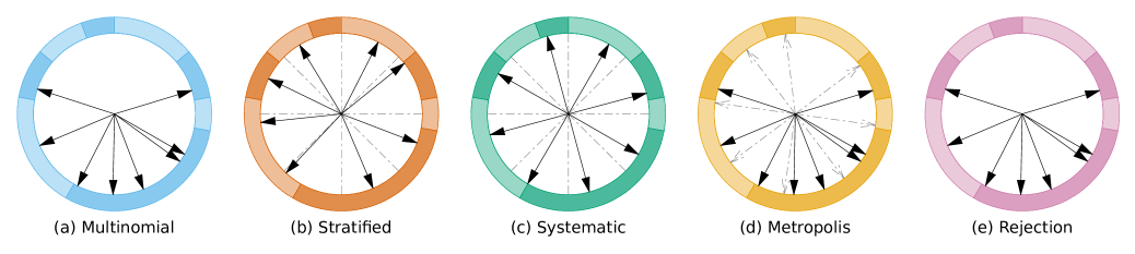
that is, the expected number of offspring of a particle should be equal to times its normalised weight. This unbiasedness condition ensures unbiased estimates of quantities such as the marginal likelihood , which follows from a simple extension of Proposition 7.4.1 in Del Moral (2004). Details of standard unbiased strategies, including their specific implementation in this work, are given in Appendix B. One common approach is to draw according to a multinomial distribution with parameters and (multinomial resampling). We will consider alternative strategies below, including some opportunities to relax the unbiasedness condition in exchange for a significant reduction in execution time. Figure 1 visualises both standard and alternative approaches.
1.2 Parallelisation
The initialisation, propagation and weighting steps of SMC are readily parallelised, being independent operations on each particle and its weight . Resampling, on the other hand, is a collective operation across particles and weights, so that parallelisation is more difficult. Summing the weights necessitates synchronization across threads, so that some threads may wastefully idle while waiting on others. For certain hardware that does not permit global communication between concurrently running threads, such as graphics processing units (GPUs), the elimination of collective operations can yield significant speed up. For this reason the resampling step has attracted recent attention as a potential bottleneck in the further scaling of SMC to larger systems (Murray, 2011; Whiteley et al., 2013).
At the core of most standard resampling schemes, such as the multinomial, stratified and systematic schemes, is a cumulative sum of weights, also called a prefix sum. A major theme of prior contributions has been the parallelisation of this prefix sum (Maskell et al., 2006; Hendeby et al., 2010; Chao et al., 2010; Gong et al., 2012). This is a generic problem that is also relevant to other algorithms (see e.g. Harris et al., 2007). Another theme in prior work is the partitioning of particles into disjoint subsets within which local resampling is performed (Chao et al., 2010). This is more useful in a distributed memory context, as it limits communication between processes (Whiteley et al., 2013); it has been considered in this context before (Brun et al., 2002; Bolić et al., 2005). General comments regarding the parallelisability of particle filtering algorithms are given in Lee et al. (2010) and Murray (2013).
1.3 Numerical precision and stability
As demonstrated later in this work, numerical instabilities can be apparent in standard resampling schemes when is large. One million particles is not an unrealistic number for some contemporary applications of SMC (see e.g. Klaas et al., 2006; Kitagawa, 2014). In double-precision, where 15 significant figures (in decimal) are expected, it is unlikely that will be sufficiently large for numerical instability to be a problem in current applications. In single-precision, however, where 8 significant figures (in decimal) are expected, numerical instabilities can manifest with this many particles. This is important because contemporary hardware has significantly faster single-precision than double-precision floating-point performance. There is reason to believe that this gap will remain; consider, for example, that single-precision is twice as fast on CPU architectures—even reasonably mature architectures—when SIMD instructions (such as those of SSE and AVX) are employed. On current GPUs, while the architecture is changing more rapidly, using single-precision also leads to at least a two-fold speedup. On other architectures, such as field-programmable gate arrays (FPGAs), custom precision is possible, allowing a trade-off between accuracy and performance (Mingas and Bouganis, 2012).
1.4 Contributions
As identified above, standard resampling algorithms require a cumulative sum over weights, leading to two problems:
-
1.
they are less readily parallelised, and
-
2.
they exhibit numerical instability for large numbers of particles or large weight variance.
This work contributes two alternative algorithms that eliminate the cumulative sum over weights in order to remedy both problems. They are better suited to the breadth of parallelism afforded by modern hardware, and do not exhibit the numerical instability of standard schemes. The two alternative schemes are based on Metropolis and rejection samplers. In comparing these to standard schemes, we carefully consider the consequences of the choice of resampling scheme on both the CPU and GPU, considering how numerical stability, bias, mean squared error and execution time vary across the number of particles and the variability in their weights. In this respect, the work constitutes a thorough study of resampling schemes and a useful guide to the selection and implementation of the most appropriate algorithm for a given problem.
Section 2 describes the Metropolis and rejection resampling schemes. We also describe a useful permutation of ancestry vectors in Section 2.3 to prevent read and write conflicts between concurrently running threads. Empirical comparisons around bias, mean squared error and execution time are given in Section 3, with concluding remarks in Section 4.
Appendix A provides our pseudocode conventions for reference. Appendix B recalls the standard algorithms for resampling based on multinomial, stratified and systematic sampling, highlighting their use of collective operations. Appendix C gives more details on the permutation algorithm. Appendix D presents auxiliary functions for converting between offspring and ancestry vectors. Appendix E provides some implementation notes.
2 Alternative resampling schemes
In this section we describe two approaches, not typically considered in the literature, that bypass the two issues shared by the standard schemes. Henceforth, we omit the subscript from weight, offspring and ancestry vectors, as the algorithms presented behave identically at each step of SMC.
2.1 Metropolis resampling
The first approach resamples via the Metropolis algorithm (Metropolis et al., 1953) rather than direct sampling, giving a result close to that of the multinomial resampler. The approach was briefly studied by the first author in a technical report (Murray, 2011), but a more complete treatment and improved analysis is given here. Instead of the collective operation, only the ratio between pairs of weights is ever computed. Code 2 describes the approach.
-
1for each 2 3 for 4 5 6 if 7 8 9return
The Metropolis resampler is parameterised by , the number of iterations to be performed before convergence is assumed and each particle may settle on its chosen ancestor. We can view the inner for loop as iterating a Markov kernel with stationary distribution for steps, where
is the categorical distribution associated with the weights.
As must be finite, the algorithm produces a biased sample. Setting is a tradeoff between speed and bias, with smaller giving faster execution time but larger bias. This bias may not be much of a problem for filtering applications, but does violate the assumptions that lead to unbiased marginal likelihood estimates in a particle MCMC framework (Andrieu et al., 2010), so care should be taken.
To provide guidance as to the selection of , we bound the total variation distance of the -fold iterate from , where
Such a bound can be obtained by noting that is an independent Metropolis Markov kernel with target and a uniform proposal on . By Theorem 2.1 of Mengersen and Tweedie (1996)
where
| (3) |
Because implies that the associated Markov chain is uniformly ergodic, and from Liu (1996), we know that the spectral gap of is exactly . To ensure that for a given it then suffices to choose
| (4) |
This requires a value or lower bound on , whose computation we would like to avoid. The bound in (3) is too weak, as it leads to setting roughly as a multiple of for large . It is sensible instead to choose as some estimate of
| (5) |
where and are respectively the mean of the weights and an upper bound on the weights. The serial complexity of the Metropolis resampler is , but may itself be a function of and the distribution of weights, as in the analysis above.
2.2 Rejection resampling
When an upper bound on the weights is known a priori, rejection sampling is possible. Like the Metropolis resampler, the rejection resampler avoids collective operations and associated numerical instability, but offers a couple of additional advantages:
-
1.
it is unbiased,
-
2.
it permits a first deterministic proposal that , increasing the probability of this outcome, and reducing the variance in the ancestry vectors produced.
Pseudocode is given in Code 3. If line 2 is replaced with (forgoing the second advantage above), rejection resampling is an alternative implementation of multinomial resampling. Its serial complexity is then .
-
1for each 2 3 4 while 5 6 7 8return
An issue unique to the rejection resampler is that the computational effort required to draw each ancestor varies, depending on the number of rejected proposals before acceptance. This is an example of a variable task-length problem (Murray, 2012), particularly acute in the GPU context. On GPUs, threads are grouped into warps and execute the same instructions in parallel. The threads in the same warp may trip the loop on line 3 of Code 3 a different number of times. All threads in the warp must complete before any thread can proceed beyond the loop. This is a particular case of warp divergence, which harms performance. A persistent threads strategy (Aila and Laine, 2009; Murray, 2012) might be used to mitigate the effects of this, although we have not been successful in finding such an implementation that does not lose more than it gains through additional overhead in register use and branching.
If line 2 of Code 3 is modified so that is sampled uniformly on then the number of iterations in the while loop is a geometric random variable with success probability given by , where is the same as that of (3), perhaps also chosen as an estimate of (5). The rejection resampler will perform poorly if this probability is small, which can occur, e.g., when . One could use the empirical maximum, , but this would require a collective operation over weights that would defeat the purpose of the approach and, moreover, could still be small.
Because of the variable task length, the serial complexity of the rejection resampling algorithm may not be as interesting as its parallel complexity. In order to determine the expected time to draw samples, we need to bound the expectation of the maximum of independent and identically distributed geometric random variables, . Such a bound is obtained in Eisenberg (2008), and we have
| (6) |
Since is the th harmonic number, we additionally have the bounds
| (7) |
and so we have that
| (8) |
Noting the inequality for , we have , and therefore that the expected parallel complexity of rejection resampling with processors is . This compares to for the Metropolis resampler with processors and set to in (4). This suggests that, if bias in the resampling step is acceptable and can be chosen appropriately, Metropolis resampling may be more appropriate than rejection resampling.
Performance can be tuned if one is willing to concede a weighted outcome from the resampling step, rather than the usual unweighted outcome. This is the approach taken with the partial rejection control heuristic (Liu et al., 1998). To do this, choose some , then form a categorical distribution using the weights , where . Clearly forms an upper bound on these new weights. One could sample from this using Code 3, with in place of , and then importance weight each particle with . Note that each weight is 1 except where . The procedure may also be used when no hard upper bound on weights exists (), but where some reasonable substitute can be made ().
2.3 Ancestor permutation for in-place propagation
A desirable feature of a resampling scheme is for it to allow in-place propagation of the particle system. This is useful for memory-intensive applications of SMC in general (Bouchard-Côté et al., 2012), but particularly for GPU implementations, since the memory available to GPU devices is typically much smaller than main memory. Instead of having an input buffer holding particles at time , and a separate output buffer into which to write the propagated particles at time , a single buffer is used with the time particles replacing the time particles. This in-place operation is more memory efficient by a factor of two (for a fixed number of particles), but requires guarantees that the reads and writes on the single buffer can be executed concurrently without conflicts. That is, each particle is either read from or written to, but not both.
To work in-place and prevent read and write conflicts, it is sufficient that the ancestry vector, , satisfies :
| (9) |
With this, it is possible to insert a copy step immediately before each propagation step, setting for all where . Each particle can then be propagated in-place by reading from and writing to the same buffer. The ancestry vector produced by resampling schemes will not typically satisfy (9), but a permutation of it will. In Appendix C we describe an algorithm to re-order the ancestry vector to achieve this, in both serial and parallel settings.
3 Results and discussion
The resampling algorithms are assessed empirically for bias, mean squared error and execution time. Single precision is used for all experiments, in order to highlight some of the numerical issues arising when standard resampling schemes are used with large numbers of particles. While the use of double precision eliminates the numerical artifacts in the results, the ranking of algorithms by execution time is unaffected.
Experiments are conducted on two devices. The first is an eight-core Intel Xeon E5-2650 CPU, compiling with the Intel C++ Compiler version 12.1.3, using OpenMP to parallelise over eight threads. The second device is an NVIDIA K20 GPU hosted by the same CPU, compiling with CUDA 5.0 and the same version of the Intel compiler. All compiler optimisations are applied. In particular, we use the -arch sm_35 option to the CUDA compiler to target the specific architecture of the NVIDIA K20.
3.1 Framework
Resampling algorithms are often assessed using the mean squared error (MSE, see e.g. Kitagawa (1996)), computed from the offspring vector and weight vector . The squared error (SE) of a particular offspring vector is:
| (10) |
For some set of offspring vectors, , the mean squared error is simply the sample mean of these squared errors: . The MSE can be written as separate bias and variance components:
| (11) |
noting:
where denotes the sample mean of the th component of across the set of offspring vectors, and the sample variance of the same. This permits separate evaluation of the bias of each resampling algorithm, recalling the unbiasedness condition (2). This is particularly important for the Metropolis resampler, which is biased for any finite number of steps, . The other algorithms have zero bias in theory, but may exhibit bias in practice due to numerical issues. Algorithms are assessed below using the contribution of the squared bias to the MSE
as well as the MSE normalised by the number of particles, .
Weight sets are simulated to assess the speed and accuracy of each resampling algorithm. For a number of particles and observation , a weight set is generated by sampling , for , and setting
| (12) |
The construction is analogous to having a prior distribution of and likelihood function of . As increases, the relative variance in weights does too. For this set up, the maximum weight is , and the expected weight
| (13) |
The variance of the weights is
| (14) |
and thus their relative variance is increasing with .
These are used to set the number of steps for the Metropolis resampler according to the analysis in Section 2.1. Using and , we set as defined in (4). The maximum weight is also used for the rejection resampler. This procedure is used to generate 16 different weight vectors for each combination of and . For each of these 16 weight vectors, each resampling algorithm is used to draw 256 offspring vectors. Results reported below are averages over the 16 weight vectors.
3.2 Bias results
Figure 2 plots the contribution of the empirical bias to the MSE for all algorithms. For the multinomial, stratified and systematic resamplers, this appears satisfactory until , after which the bias contribution increases rapidly. This is due to the numerical instability of the cumulative sum required by these algorithms. The instability is noticeably worse for the different multinomial algorithm used on the CPU (Code 6 in Appendix B.1) than that on the GPU (Code 5 in Appendix B.1); this is explained by the cumulative sum in the former being linear over a vector rather than recursive over a binary tree. The Metropolis and rejection algorithms do not share this instability, and otherwise empirically match the bias contribution of the other methods. This is to be expected for the rejection algorithm. For the Metropolis algorithm it suggests that the procedure for setting in Section 2.1 is appropriate. It also suggests that while the Metropolis algorithm is theoretically biased, this bias is negligible in practice compared to numerical errors.
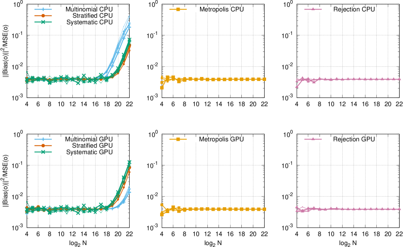
We observe, but do not show, that the pre-sorting of weights does not fix the numerical instability of the multinomial, stratified and systematic resamplers for large numbers of particles, but that the use of double precision does. The number of particles that would be required to reproduce the same instability in double precision far surpasses, by orders of magnitude, that which would be realistic to use in SMC at present.
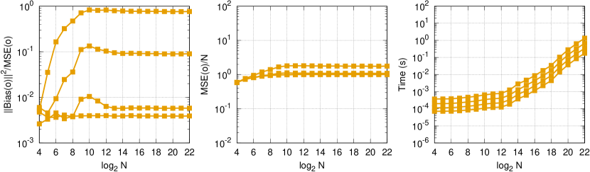
The selection of for the Metropolis resampler appears sufficient, but we may question whether it is too conservative. To test this empirically we compare runs of the Metropolis resampler with reduced number of steps, setting for each . The contribution of the empirical bias to the MSE is given in the leftmost plot of Figure 3. As it matches that of the multinomial resampler for —which cannot be improved upon—and noticeably increases for , this suggests that the setting is indeed appropriate.
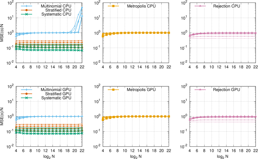
3.3 MSE results
Figure 4 indicates that MSE differs between methods. Little in this figure is surprising, however: it is well known that the stratified resampler reduces variance over the multinomial resampler, and that the systematic resampler can, but does not necessarily, reduce it again (Douc and Cappé, 2005). Numerical instabilities in the CPU implementation of the multinomial resampler (Code 6 in Appendix B.1) appear to increase the MSE in its outcomes for large . Also of interest is that as increases, the probability of accepting the initial proposal of the rejection resampler declines, so that its MSE degrades away from that of the systematic and stratified resamplers, towards that of the multinomial and Metropolis resamplers.
3.4 Execution time results
Figure 5 shows the execution times for all algorithms, as well as, for context, the execution times of procedures for sorting a weight vector and computing its effective sample size (ESS) (Liu and Chen, 1995). The ESS is given by .
Execution times are taken until the delivery of an ancestry vector satisfying (9), and so include any of the auxiliary functions in Appendices D and C necessary to achieve this. Note that—as we would expect—the multinomial, stratified and systematic resamplers are not sensitive to (or equivalently to the variance in weights) with respect to execution time, while the Metropolis and rejection resamplers are.
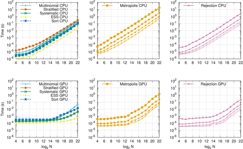
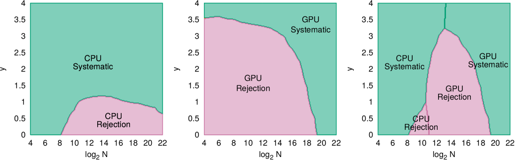
In a Bayesian decision theoretic setting, we can adopt execution time as a loss function, and choose, for any combination of and , the algorithm that minimises the expectation of this loss function. A more sophisticated loss function might include the bias and variance as well, but the relative weighting of the individual components is a subjective decision for the problem at hand, so we do not attempt to do this. Using execution time alone as a loss function, Figure 6 plots the resulting decision matrices across all combinations of and for which empirical results were recorded. From these matrices and Figure 5, we can conclude:
-
1.
that the GPU should generally not be considered for resampling with fewer than particles,
-
2.
that the systematic resampler is a good candidate overall, but
-
3.
that there is a significant region of the space, especially at lower weight variances, for which the rejection or Metropolis resamplers are faster.
We observe, but do not show, that the decision boundaries in Figure 6 are not significantly affected by including the time taken to copy between GPU device and main memory. This means that the choice between the CPU or GPU device for resampling is largely independent of the choice of device for the propagation and weighting of particles. For example, use of the GPU for propagating and weighting particles does not then greatly favour the GPU for resampling: the penalty to copy the weight vector to main memory, resample using the CPU, and then copy the resulting ancestry vector back to device memory, is not significant.
The choice of for the Metropolis algorithm permits a trade off between bias and execution time. This may be particularly useful in applications with hard execution time constraints, such as real-time object tracking. Recall that execution time is linear in . Execution time results for various choices of are given in the rightmost plot of Figure 3, with associated biases in the leftmost plot. Recall that the rejection resampler is also somewhat configurable by using an approximate maximum weight. To do this, one must be willing to accept a still-weighted output from the resampling step, and the cumulative implications of this within SMC are problem-specific and not overly clear. We leave this for future work.
A further consideration is that the execution time of both the Metropolis and rejection resamplers depends on the PRNG used. This dependence is by a constant factor, but can be substantial. Here, robust PRNGs for Monte Carlo work have been used (see Appendix E), but conceivably cheaper, if less robust, PRNGs might be considered. This represents another trade-off between execution time and bias.
4 Conclusion
This work has presented two alternative resampling schemes for SMC that eliminate collective operations over weights. Consequently, they are more readily parallelised and are more numerically stable than standard resampling schemes.
The appropriate choice of resampling algorithm depends on a number of problem-specific factors, including:
-
1.
the number of particles required and the typical variability in their associated weights,
-
2.
whether a maximum weight exists, or can be approximated sufficiently accurately, to configure and use the Metropolis and rejection algorithms,
-
3.
the tolerable level of bias in resampling outcomes, and
-
4.
the available numerical precision.
The Metropolis and rejection algorithms:
- 1.
-
2.
allow a practitioner to implement SMC in single precision for large numbers of particles without the numerical instabilities of existing resampling schemes.
With respect to numerical stability, especially in single precision, great care should be taken when using the standard multinomial, stratified or systematic resamplers with upwards of hundreds of thousands of particles, even though these schemes are unbiased in theory. This is due to numerical instability in the cumulative sum operation that these algorithms require. The alternative Metropolis and rejection resamplers have better numerical properties, as they compute only ratios of weights. This is important in light of the temptation to use single-precision, or even custom-precision floating point to improve execution times with modern computer architectures.
Supplementary materials
- LibBi package for numerical results:
-
LibBi package Resampling providing scripts to reproduce the numerical results of this article using all algorithms as implemented in the LibBi software, available at www.libbi.org.
Acknowledgements
The third author acknowledges EPSRC for funding this research through grant EP/K009362/1.
References
- Aila and Laine (2009) Aila, T. and S. Laine (2009). Understanding the efficiency of ray traversal on GPUs. In Proc. High-Performance Graphics 2009, pp. 145–149.
- Andrieu et al. (2010) Andrieu, C., A. Doucet, and R. Holenstein (2010). Particle Markov chain Monte Carlo methods. Journal of the Royal Statistical Society B 72, 269–302.
- Bell and Hoberock (2012) Bell, N. and J. Hoberock (2012). Chapter 26 - Thrust: A productivity-oriented library for CUDA. In W. W. Hwu (Ed.), GPU Computing Gems Jade Edition, Applications of GPU Computing Series, pp. 359–371. Boston: Morgan Kaufmann.
- Bentley and Saxe (1979) Bentley, J. L. and J. B. Saxe (1979). Generating sorted lists of random numbers. Technical Report 2450, Carnegie Mellon University, Computer Science Department.
- Bolić et al. (2005) Bolić, M., P. M. Djurić, and S. Hong (2005). Resampling algorithms and architectures for distributed particle filters. IEEE Transactions on Signal Processing 53, 2442–2450.
- Bouchard-Côté et al. (2012) Bouchard-Côté, A., S. Sankararaman, and M. I. Jordan (2012). Phylogenetic inference via sequential Monte Carlo. Systematic Biology, syr131.
- Brun et al. (2002) Brun, O., V. Teuliere, and J.-M. Garcia (2002). Parallel particle filtering. Journal of Parallel and Distributed Computing 62(7), 1186 – 1202.
- Cérou et al. (2012) Cérou, F., P. Del Moral, T. Furon, and A. Guyader (2012). Sequential monte carlo for rare event estimation. Statistics and Computing 22(3), 795–808.
- Chao et al. (2010) Chao, M.-A., C.-Y. Chu, C.-H. Chao, and A.-Y. Wu (2010, Oct). Efficient parallelized particle filter design on CUDA. In Signal Processing Systems (SIPS), 2010 IEEE Workshop on, pp. 299–304.
- Chopin (2002) Chopin, N. (2002). A sequential particle filter method for static models. Biometrika 89(3), 539–552.
- Chopin and Jacob (2010) Chopin, N. and P. E. Jacob (2010). Free energy sequential monte carlo, application to mixture modelling. In Bayesian Statistics 9: proceedings of the Ninth Valencia International Meeting.), pp. 91–118.
- Del Moral (2004) Del Moral, P. (2004). Feynman-Kac Formulae: Genealogical and Interacting Particle Systems with Applications. Springer–Verlag.
- Del Moral et al. (2006) Del Moral, P., A. Doucet, and A. Jasra (2006). Sequential Monte Carlo samplers. Journal of the Royal Statistical Society B 68, 441–436.
- Douc and Cappé (2005) Douc, R. and O. Cappé (2005, 15-17). Comparison of resampling schemes for particle filtering. In Image and Signal Processing and Analysis, 2005. ISPA 2005. Proceedings of the 4th International Symposium on, pp. 64 – 69.
- Doucet et al. (2001) Doucet, A., N. de Freitas, and N. Gordon (Eds.) (2001). Sequential Monte Carlo Methods in Practice. Springer–Verlag.
- Eisenberg (2008) Eisenberg, B. (2008). On the expectation of the maximum of IID geometric random variables. Statistics & Probability Letters 78(2), 135 – 143.
- Gong et al. (2012) Gong, P., Y. Basciftci, and F. Ozguner (2012, May). A parallel resampling algorithm for particle filtering on shared-memory architectures. In Parallel and Distributed Processing Symposium Workshops PhD Forum (IPDPSW), 2012 IEEE 26th International, pp. 1477–1483.
- Gordon et al. (1993) Gordon, N., D. Salmond, and A. Smith (1993). Novel approach to nonlinear/non-Gaussian Bayesian state estimation. IEE Proceedings-F 140, 107–113.
- Harris et al. (2007) Harris, M., S. Sengupta, and J. D. Owens (2007). GPU Gems 3, Chapter Parallel Prefix Sum (Scan) with CUDA. NVIDIA.
- Hendeby et al. (2010) Hendeby, G., R. Karlsson, and F. Gustafsson (2010). Particle filtering: The need for speed. EURASIP Journal on Advances in Signal Processing 2010, 1–9.
- Hoberock and Bell (2010) Hoberock, J. and N. Bell (2010). Thrust: A parallel template library.
- Kalman (1960) Kalman, R. (1960). A new approach to linear filtering and prediction problems. Journal of Basic Engineering 82, 35–45.
- Kitagawa (1996) Kitagawa, G. (1996). Monte Carlo filter and smoother for non-Gaussian nonlinear state space models. Journal of Computational and Graphical Statistics 5, 1–25.
- Kitagawa (2014) Kitagawa, G. (2014). Computational aspects of sequential Monte Carlo filter and smoother. Annals of the Institute of Statistical Mathematics, 1–29.
- Klaas et al. (2006) Klaas, M., M. Briers, N. de Freitas, A. Doucet, S. Maskell, and D. Lung (2006). Fast particle smoothing: If I had a million particles. Proceedings of the 23rd International Conference on Machine Learning.
- L’Ecuyer and Simard (2007) L’Ecuyer, P. and R. Simard (2007). TestU01: A C library for empirical testing of random number generators. ACM Transactions on Mathematical Software 33.
- Lee et al. (2010) Lee, A., C. Yau, M. B. Giles, A. Doucet, and C. C. Holmes (2010). On the utility of graphics cards to perform massively parallel simulation of advanced Monte Carlo methods. Journal of Computational and Graphical Statistics 19, 769–789.
- Liu (1996) Liu, J. S. (1996). Metropolized independent sampling with comparisons to rejection sampling and importance sampling. Statistics and Computing 6(2), 113–119.
- Liu and Chen (1995) Liu, J. S. and R. Chen (1995). Blind deconvolution via sequential imputations. Journal of the American Statistical Association 90, 567–576.
- Liu and Chen (1998) Liu, J. S. and R. Chen (1998). Sequential Monte-Carlo methods for dynamic systems. Journal of the American Statistical Association 93, 1032–1044.
- Liu et al. (1998) Liu, J. S., R. Chen, and W. H. Wong (1998). Rejection control and sequential importance sampling. Journal of the American Statistical Association 93(443), 1022–1031.
- Marsaglia (1996) Marsaglia, G. (1996). DIEHARD: a battery of tests of randomness.
- Marsaglia (2003) Marsaglia, G. (2003). Xorshift RNGs. Journal of Statistical Software 8(14), 1–6.
- Maskell et al. (2006) Maskell, S., B. Alun-Jones, and M. Macleod (2006, Sept). A single instruction multiple data particle filter. In Nonlinear Statistical Signal Processing Workshop, 2006 IEEE, pp. 51–54.
- Matsumoto and Nishimura (1998) Matsumoto, M. and T. Nishimura (1998). Mersenne twister: A 623-dimensionally equidistributed uniform pseudorandom number generator. ACM Transactions on Modeling and Computer Simulation 8, 3–30.
- Mengersen and Tweedie (1996) Mengersen, K. L. and R. L. Tweedie (1996). Rates of convergence of the Hastings and Metropolis algorithms. The Annals of Statistics 24(1), 101–121.
- Metropolis et al. (1953) Metropolis, N., A. Rosenbluth, M. Rosenbluth, A. Teller, and E. Teller (1953). Equation of state calculations by fast computing machines. Journal of Chemical Physics 21, 1087–1092.
- Mingas and Bouganis (2012) Mingas, G. and C.-S. Bouganis (2012). A custom precision based architecture for accelerating parallel tempering MCMC on FPGAs without introducing sampling error. In IEEE 20th International Symposium on Field-Programmable Custom Computing Machines.
- Murray (2011) Murray, L. M. (2011). GPU acceleration of the particle filter: The Metropolis resampler. In DMMD: Distributed machine learning and sparse representation with massive data sets.
- Murray (2012) Murray, L. M. (2012). GPU acceleration of Runge–Kutta integrators. IEEE Transactions on Parallel and Distributed Systems 23, 94–101.
- Murray (2013) Murray, L. M. (2013). Bayesian state-space modelling on high-performance hardware using LibBi. In review.
- Naesseth et al. (2014) Naesseth, C. A., F. Lindsten, and T. B. Schön (2014). Sequential Monte Carlo for graphical models. In Advances in Neural Information Processing Systems, pp. 1862–1870.
- Nandapalan et al. (2012) Nandapalan, N., R. P. Brent, L. M. Murray, and A. P. Rendell (2012). High-performance pseudo-random number generation on graphics processing units. In R. Wyrzykowski, J. Dongarra, K. Karczewski, and J. Waśniewski (Eds.), Parallel Processing and Applied Mathematics, Volume 7203 of Lecture Notes in Computer Science, pp. 609–618. Springer–Verlag.
- NVIDIA Corporation (2012) NVIDIA Corporation (2012, July). CUDA Toolkit 5.0 CURAND Library. NVIDIA Corporation.
- Satish et al. (2009) Satish, N., M. Harris, and M. Garland (2009, May). Designing efficient sorting algorithms for manycore GPUs. In Parallel Distributed Processing, 2009. IPDPS 2009. IEEE International Symposium on, pp. 1–10.
- Schäfer and Chopin (2013) Schäfer, C. and N. Chopin (2013). Sequential monte carlo on large binary sampling spaces. Statistics and Computing 23(2), 163–184.
- Schweizer (2012) Schweizer, N. (2012). Non-asymptotic error bounds for sequential mcmc methods in multimodal settings. arXiv preprint arXiv:1205.6733.
- Whiteley et al. (2013) Whiteley, N., A. Lee, and K. Heine (2013). On the role of interaction in sequential Monte Carlo algorithms.
- Zhou et al. (2013) Zhou, Y., A. M. Johansen, and J. A. Aston (2013). Towards automatic model comparison: an adaptive sequential monte carlo approach. arXiv preprint arXiv:1303.3123.
Appendix A Pseudocode conventions
The algorithms presented in this work are described using pseudocode with a number of conventions. We distinguish between the for each and for constructs. The former is used where the body of the loop is to be executed for each element of a set, with the order unimportant. The latter is used where the body of the loop is to be executed for each element of a sequence, where the order must be preserved. The intended implication is that for each loops may be parallelised, while for loops cannot be. The atomic keyword is used to indicate that a line must be executed as if it constitutes one instruction (i.e. an atomic operation) in order to avoid read and write conflicts between concurrently running threads.
A number of primitive operations such as searches, transformations, reductions, sorts and prefix sums are used throughout pseudocode. These are specified in Code 4. Such operations will be familiar to users of, for example, the C++ standard template library (STL) or Thrust library (Hoberock and Bell, 2010), and their implementation on GPUs has been well-studied (see e.g. Harris et al., 2007; Satish et al., 2009). The advantage of describing algorithms in this way is that we can specify intent without prescribing implementation; the efficient implementation of these primitives in both serial and parallel contexts is well understood, and a single pseudocode description that uses primitives will often suffice for both serial and parallel contexts.
-
1 2return
-
1 2return
-
1 2return
-
1return
-
1requires 2 is sorted in ascending order 3return 4 the lowest such that may be inserted into position of and maintain its sorting.
Appendix B Standard resampling schemes
B.1 Multinomial resampling
Multinomial resampling proceeds by drawing each independently from the categorical distribution over , where . Pseudocode is given in Code 5. The algorithm is dominated by the calls of Lower-Bound, which if implemented with a binary search, will give a serial complexity of overall.
-
1 2for each 3 4 5return
The Inclusive-Prefix-Sum operation on line 5 of Code 5 is not numerically stable, as large values may be added to relatively insignificant ones during the procedure (an issue intrinsic to any large summation). With large , assigning the weights to the leaves of a binary tree and summing with a depth-first recursion over this will help. With large variance in weights, pre-sorting may also help. While log-weights are often used in the implementation of SMC, these need to be exponentiated (perhaps after rescaling) for the Inclusive-Prefix-Sum operation, so this does not alleviate the issue.
Serially, the same approach may be used, although a single-pass approach of complexity is enabled by generating sorted uniform random variates (Bentley and Saxe, 1979). Code 6 details this approach. A drawback is the use of relatively expensive logarithm functions. There is scope for a small degree of parallelism in this new algorithm by dividing among a handful of threads. Each thread must still step through all weights, however, so that the complexity is not improved with parallelism. We find it faster than Code 5 when on CPU, but slower when on GPU.
-
1 2 // sum of weights 3 4 5for 6 7 8 9 while 10 11 12return
B.2 Stratified resampling
The variance in outcomes produced by the multinomial resampler may be reduced (Douc and Cappé, 2005) by stratifying the cumulative probability function of the same categorical distribution, and randomly drawing one particle from each stratum. This stratified resampler (Kitagawa, 1996) most naturally delivers not the ancestry vector or offspring vector , but the cumulative offspring vector, which we denote , and define as . Pseudocode is given in Code 7. The algorithm is of serial complexity .
-
1 2 3for each 4 5 6 7return
As for multinomial resampling, the Inclusive-Prefix-Sum operation on line 7 of Code 7 is not numerically stable. The same strategies to ameliorate the problem apply. Line 7 of Code 7 is more problematic. Consider that there may be a such that, for , is not significant against under the floating-point model, so that the result of is just . For such , no random sample is being made within the strata. Furthermore, rounding up on the same line might easily deliver , not as required, if not for the quick-fix use of . Given that single precision has about seven significant figures in decimal, consider that, with around one million, almost certainly no is significant against at high . Note that while pre-sorting weights and summing over a binary tree can help with the numerical stability of the Inclusive-Prefix-Sum operation, it does not help with this latter issue.
B.3 Systematic resampling
The variance in outcomes of the stratified resampler may often, but not always (Douc and Cappé, 2005), be further reduced by using the same random offset within each stratum. This is the systematic resampler (equivalent to the deterministic method described in the appendix of Kitagawa (1996)). Pseudocode is given in Code 8, which is a simple modification to Code 7. The same complexity and numerical caveats apply to the systematic resampler as for the stratified resampler.
-
1 2 3for each 4 5 6return
The resampling algorithms presented here do not constitute an exhaustive list of those in use, for instance residual resampling has been omitted (Liu and Chen, 1998). However they are reasonably representative, and can form the building blocks of more elaborate schemes.
Appendix C Ancestor permutation for in-place propagation
An ancestry vector may be permuted to satisfy (9) in the main article. A serial algorithm to achieve this is straightforward and given in Code 9. This algorithm makes a single pass through the ancestry vector with pair-wise swaps to satisfy the condition.
-
1for 2 if and 3 4 // repeat for new value 5ensures 6
The simple algorithm is complicated in a parallel context as the pair-wise swaps are not readily serialised without heavy-weight mutual exclusion. In parallel we propose Code 10. This algorithm does not perform the permutation in-place, but instead produces a new vector that is the permutation of the input vector . It introduces a new vector , through which, ultimately, . In the first stage of the algorithm, Prepermute, the thread for element attempts to claim position in the output vector by setting . By virtue of the function on line 10, the element of lowest index always succeeds in this claim while all others contesting the same place fail, and the outcome of the whole permutation procedure is deterministic. This is desirable so that the results of a particle filter are reproducible for the same pseudorandom number seed. For each element that is not successful in its claim, the thread for instead attempts to claim , if unsuccessful again then , then recursively etc, until an unclaimed place is found.
-
1Let and set for . 2for each 3 atomic // attempt to claim this slot, minimum is winner 4ensures 5 6return
-
1 2for each 3 4 if // if claim was unsuccessful in Prepermute 5 6 while 7 8 9for each 10 11ensures 12 13return
We offer a proof of the termination of Code 10. First note that Prepermute leaves in a state where, excluding all values of , the remaining values are unique. Furthermore, in Permute the conditional on line 10 means that the loop on line 10 is only entered for values of that are not represented in .
For each such , the while loop traverses the sequence , , until . For the procedure to terminate this sequence must be finite. Because each is an element of the finite set , to show that the sequence is finite it is sufficient to show that it never revisits the same value twice. The proof is by induction.
Proof.
-
1.
As no value of is , the sequence cannot revisit its initial value . The element is therefore unique.
-
2.
For , assume that the elements of are unique.
-
3.
Now, the elements of are not unique if there exists some such that , with by the uniqueness of . But this contradicts the uniqueness of the (non ) values of . Thus the elements of are unique, the sequence is finite, and the program must terminate.
∎
Appendix D Auxiliary functions
The multinomial, Metropolis and rejection resamplers most naturally return the ancestry vector , while the stratified and systematic resamplers return the cumulative offspring vector . Conversion between these is reasonably straightforward. An offspring vector may be converted to a cumulative offspring vector via the Inclusive-Prefix-Sum primitive, and back again via Adjacent-Difference. A cumulative offspring vector may be converted to an ancestry vector via Code 11, and an ancestry vector to an offspring vector via Code 12. These functions perform well on both CPU and GPU. An alternative approach to Cumulative-Offspring-To-Ancestors, using a binary search for each ancestor, was found to be slower.
-
1for each 2 if 3 4 else 5 6 7 for 8 9return
-
1 2for each 3 atomic 4return
Appendix E Implementation
All the algorithms described in the article and the appendices have been implemented as part of the LibBi software (www.libbi.org, Murray (2013)) for performing methods such as the particle filter on high-performance computing devices. We enumerate the most important considerations of the implementation here, and avoid painstaking detail of the remainder so as not to oversell their importance relative to these. It is worth emphasising that some important decisions, such as the choice of pseudorandom number generator (PRNG), depend on the particular problem at hand.
The weight vector may contain many very small values. Because of this, a typical implementation will store log-weights rather than weights for numerical accuracy. The log-weights may be large and negative, and one should avoid taking a floating point exponential of these large negative numbers, which is often zero. All of the algorithms presented are robust to the scaling of weights by a constant factor, however. When computing sums or prefix sums, a vector of log-weights can therefore be renormalised using, say, the maximum value, denoted . For example, the logarithm of the sum of weights, stored as log-weights, is accurately computed using the identity:
Renormalisation is not required for the Metropolis and rejection algorithms, as they feature only pairwise ratios between weights, or pairwise differences between log-weights.
The performance of the multinomial, stratified and systematic resamplers depends largely on the implementation of the prefix sum operation. We defer to existing work for these operations, in particular to that invested in the Thrust library (Bell and Hoberock, 2012), which the implementation uses. Conceptually, the implementation in the Thrust library is based on up- and down-sweeps of a balanced binary tree (Harris et al., 2007).
The performance of the Metropolis and rejection resamplers is dependent mostly on the selection of PRNG. Performance is not the only consideration in this selection, however. PRNGs are assessed both on execution speed and the statistical quality of the pseudorandom number sequence that they produce, typically using test suites such as DIEHARD (Marsaglia, 1996) or TestU01 (L’Ecuyer and Simard, 2007). Among clients of PRNGs, Monte Carlo algorithms, such as the particle filter, have high demands for statistical quality. To this end, our CPU code uses the Mersenne Twister PRNG (Matsumoto and Nishimura, 1998) as implemented in the Boost.Random library (www.boost.org). This is standard for Monte Carlo applications. Our GPU code uses the XORWOW PRNG (Marsaglia, 2003) from the CURAND library (NVIDIA Corporation, 2012). This particular PRNG belongs to a family that is readily shaped to the GPU architecture (Nandapalan et al., 2012). Faster but lower quality PRNG may be used. This would constitute a relaxing of the unbiasedness condition (2). As any such decision is problem-specific, it is not investigated in this work.
The Metropolis and rejection algorithms use random access patterns to memory. Spatiotemporally local access patterns are preferred for good cache performance on CPU, and streaming, or at least coalesced access, is preferred on GPU. The random access pattern is, unfortunately, inherent to the algorithms, and we can only rely on the presence of a large cache to mitigate associated latencies. On GPU, juditious use of shared memory may help, but there is no reason to believe that this can achieve better results than the hardware-controlled cache found on more recent architectures; we rely on the latter. As such, the GPU is configured to use 48 KB of L1 cache and 16 KB of shared memory. This maximises the size of the cache for random access patterns, but still provides sufficient shared memory for all kernels.
Our Metropolis and rejection resampler kernels compile to 32 registers per thread, as reported by the CUDA compiler. This is satisfactory with respect to occupancy of the device, and we do not seek further reductions.
Finally, the auxiliary algorithms presented in §D pose little challenge. Implemented using CUDA, they compile to kernels using no shared memory and fewer than 16 registers per thread, which is of no hindrance to occupancy of the device. On GPU, we append the Prepermute procedure of Code 10 to the end of any procedure that produces an ancestry vector. This saves the launch of a separate kernel and the associated overhead of doing so.