According to the Anderson theorem, the critical temperature $T_{c}$ of a disordered superconductor is determined by the average density of states and does not change at the localization threshold. This statement is valid under assumption of a self-averaging order parameter, which can be violated in the strong localization region. Stimulating by statements on the essential increase of $T_{c}$ near the Anderson transition, we carried out the systematic investigation of possible violations of self-averaging. Strong deviations from the Anderson theorem are possible due to resonances at the quasi-discrete levels, resulting in localization of the order parameter at the atomic scale. This effect is determined by the properties of individual impurities and has no direct relation to the Anderson transition. In particular, we do not see any reasons to say on ”fractal superconductivity” near the localization threshold.

The general picture of coexistence of superconductivity and the Anderson localization was formed in the papers by Bulaevskii and Sadovskii [1]–[5] (see also [6, 7]). According to the Anderson theorem [8], the critical temperature $T_{c}$ of a disordered superconductor is determined by the average density of states and does not depend on the form of one-particle eigenstates. Since the average density of states does not have singularity at the Anderson transition, so $T_{c}$ has the analogous behavior. The coefficient of the gradient term in the Ginzburg–Landau expansion, determining the superconducting response of the system, remains finite at the critical point. In the localized phase, the system breaks up into quasi-independent blocks of size $\xi$ ($\xi$ is the localization length) and superconductivity is suppressed due to the size effect, when the average level spacing in such a block becomes greater than $T_{c}$.

Recently it was stated by Feigelman et al [9, 10] that $T_{c}$ increases at approaching the Anderson transition from the metallic side and continues to grow in the localized phase (with a maximum in the deep of it); it is related with multifractality of wave functions. More than that, $T_{c}$ depends on the Cooper interaction constant $g$ not exponentially, but in the power-law manner. Formally, this statement does not contradict to the papers [1]–[5]. Indeed, the Anderson theorem is valid under assumption of a self-averaging character of the order parameter, which in fact reduces to its spatial uniformity. According to estimates of [3, 4], the self-averaging property tends to violate when the localization threshold is approached and the space-inhomogeneous superconductivity is expected in the deep of the localization phase; so the true $T_{c}$ can be greater than its value given by the Anderson theorem. In fact, controversy between the papers [1]–[5] and [9, 10] has an ideological character. The authors of [1]–[5] proceed from the standpoint that localization counteracts to superconductivity, so the latter encounters a lot of problems in the localized phase [2, 5]. Contrary, the growth of $T_{c}$ after the mobility edge [9, 10] indicates that superconductivity not only ”survives” but even ”prospers” in the localized phase. It looks suspicious from the physical viewpoint and contradicts the experimental situation, which is in complete agreement with [1]–[5].

The present paper has an aim to clarify a situation. In fact, the essence of the problem is: how and in what extent self-averaging of the order parameter can be violated? The efficient approach to such problems was developed in [11]–[14] and consists in the study of individual defects and their influence on the transition temperature. In particular, for the plane defects arranged perpendicularly to the $z$ axis with the period $L$ along it, the change of $T_{c}$ is determined by the formula 

$$\frac{\delta T_{c}}{T_{c0}}=\frac{1}{\lambda_{0}^{3}L}\,g^{2}\!\int dz\left[\nu_{0}\nu_{1}(z)+\nu_{1}(z)^{2}\right]\,,$$

if there are no surface states localized near defects. Here $g$ is the Cooper interaction constant, $\nu_{1}(z)$ is a deviation of the local density of states $\nu(z)$ from its unperturbed value $\nu_{0}$, $\lambda_{0}=g\nu_{0}$ is the dimensionless coupling constant, $T_{c0}$ is the transition temperature in the absence of defects, integration is carried out over a vicinity of the single defect. For weak defects, only the linear in $\nu_{1}(z)$ term is essential, which exactly corresponds to the Anderson theorem and relates the change in $T_{c}$ with the change of the average density of states. Generally, $\nu_{1}(z)$ is comparable with $\nu_{0}$ and already Eq.1 predicts a possibility of essential violation of the Anderson theorem. It is related with the fact that the initially uniform order parameter is influenced by strong defects and can increase or decrease in their vicinity. More essential violations of the Anderson theorem are possible, if the surface states localized near defect appear at the Fermi level (Fig.1).

Figure 1: If plane defects are arranged perpendicular to the $z$ axis, the problem allows a separation of variables and the longitudinal quasi-momentum $k_{\parallel}$ can be introduced. For fixed $k_{\parallel}$, the spectrum is a set of bands with discrete levels splitted from them; if dependence on $k_{\parallel}$ is taken into account, these levels turn into $2D$ bands, which can appear at the Fermi level.

In this case, the order parameter can be strongly localized near the plane defects, so $T_{c}$ does not depend on $L$ and is determined by the BCS formula $T_{c}=1.14\omega_{0}\exp(-1/\lambda_{2D})$ with the coupling constant $\lambda_{2D}$, corresponding to the separated two-dimensional band (Fig.1). A crossover between two regimes is appeared to be very sharp and the intermediate situation is of little interest. Formally, the described results correspond to the periodical arrangement of defects, but their character shows that the assumption on periodicity is not essential; so they give a complete picture for the small ”impurity” concentration in the 1D geometry.

Analogous effects are possible in case of the point defects, where the localized regime for the order parameter is related with existence of the quasi-local states (Fig.2). A detailed investigation of these effects allows to obtain the complete picture of possible violations of self-averaging. The main conclusion is that such violations are determined by individual defects and have no direct relation to the Anderson transition. One can distinguish two typical situations.

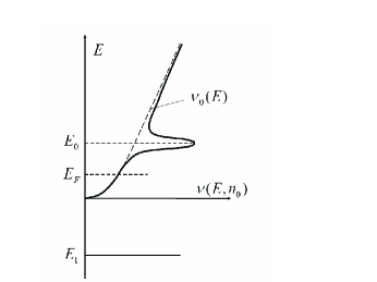
Figure 2: A strong point defect inserted into site $n_{0}$ of an ideal lattice leads to appearance of the local ($E_{1}$) and quasi-local ($E_{0}$) levels. The latter corresponds to the maximum of the local density of states $\nu(E,n_{0})$.

If disorder is created by weak impurities (Fig.3, a), then

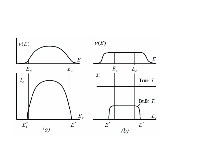
Figure 3: (a) If disorder is created by weak impurities, self-averaging of the order parameter is not violated; $T_{c}$ strongly falls near the mobility edge due to decrease of the density of states. (b) In case of strong disorder, the true $T_{c}$ is determined by localization of the order parameter at rare resonant impurities, while the ”bulk $T_{c}$” obeys to the ”rectangular” dependence.

the assumption of self-averaging is always true and the Bulaevskii–Sadovskii picture is literally applicable. The mobility edge lies near the initial band edge and $T_{c}$ is falling quickly at approaching it from the metal side due to decrease of the density of states; hence, superconductivity becomes practically unobservable before the mobility edge is reached. Such situation is typical for the traditional superconductors, which are good metals and effectively screen any impurity which is introduced in them. The experimental situation is in complete agreement with these considerations [5].

In case of strong disorder (Fig.3,b), the mobility edge can be located in the region of the practically uniform density of states , so the $T_{c}$ value given by the Anderson theorem does not fall in approaching the localization threshold. In fact, the true $T_{c}$ appears to be much larger and corresponds to localization of the order parameter at the small number of the ”resonant” impurities, which produce the quasi-local states near the Fermi level. In accordance with papers [9, 10], $T_{c}$ depends on the interaction constant $g$ in the power-law manner, but contrary to them, it has no essential dependence on the Fermi level position. It removes an illusion that localization ”helps” superconductivity. In the vicinity of the true $T_{c}$, observation of superconductivity is practically impossible due to a small fraction of the Meissner phase and negligible values of the critical current. Superconductivity becomes easily observable when it spreads to the whole volume: it occurs at some effective temperature, which we refer as the ”bulk $T_{c}$”; it can be defined theoretically as a transition temperature of the system with removed ”resonant” impurities. Such ”bulk $T_{c}$” corresponds qualitatively (but not quantitatively) to the Anderson theorem and the Bulaevskii–Sadovskii picture is confirmed at this level. In such a case, $T_{c}$ obeys the ”rectangular” dependence (Fig.3,b), which exponentially weakly deviates from the horizontal line near the mobility edge $E_{c}$, and exponentially weakly deviates from the vertical line near the endpoint $E^{*}$ of superconductivity. Such situation is typical for high $T_{c}$ superconductors, where coexistence of localization and superconductivity is easily observable [5].

The estimate for the true $T_{c}$

$$T_{c}\sim ga^{-d}\sim\lambda_{0}J$$

($a$ is the lattice spacing, $J$ is a bandwidth, and $d$ is the space dimension) gives an impression that the ”room” superconductivity is a widespread phenome- non. In fact, the growth of $T_{c}$ with the increase of $\lambda_{0}$ is bounded by a quantity $\omega_{0}/\pi$, where $\omega_{0}$ is a cut-off frequency. For the phonon mechanism, such upper bound corresponds to the values already attained in high $T_{c}$ superconductors, and their further increase requires the use of higher frequency Bose excitations. In addition, the observation of true $T_{c}$ is probably possible only with the use of the scanning tunnel or squid microscopy [16].

It should be stressed that Eq.2 is a result of the mean field theory. The corresponding solution for the order parameter shows existence of the certain uniform contribution with abrupt peaks near the rare resonant impurities (with concentration $T_{c}/J$). The order parameter can be considered as positive (see Sec.2) and so its phase is constant in the whole volume. In the fluctuational theory, the modulus of the order parameter remains practically unchanged, while the essential phase fluctuations arise. If the uniform contribution is neglected, then the system is divided into practically independent superconducting ”drops”, whose phases are fluctuating freely and destroy the macroscopical coherence of the superconducting state. If the uniform contibution is taken into account, the Josephson coupling between drops arises and their phases become correlated. The accurate fluctuational analysis of such a system is nontrivial, but the general character of results is the same as for the granual superconductors [17]. If the ratio $T_{c}/J$ is not too small, then the resonant impurities are close to each other and their Josephson interaction is strong enough for stabilization of the mean-field solution at practically the same $T_{c}$ value (in this sense it can be qualified as ”true”); if a concentration of the resonant impurities appears to be small, then $T_{c}$ is suppressed by fluctuations to the value somewhat greater than the ”bulk $T_{c}$” (Sec. 7).

According to the results of [9, 10] 

$$T_{c}\sim g^{1/\gamma}\,,\qquad f\sim(T_{c}/J)^{\gamma}\,,$$

where $f$ is a portion of volume occupied by superconductivity, and parameter $\gamma=0.57$ is related with a fractal dimensionality of wave functions. We do not deny the existence of the order parameter configurations, leading to results of type (3) (Sec.3), but Eq.2 corresponds to the higher value of $T_{c}$; the corresponding configuration of the order parameter is determined by the rare peaks near the resonant impurities, occuring at the atomic scale and occupying a portion of volume $f\sim T_{c}/J$. If superconductivity is considered as a variational problem, then it is possible to say that our trial function is more successful than one in [9, 10]. Formally, our results correspond to Eq.3 with $\gamma=1$ and do not contain any information on multifractality; hence, there are no grounds to say on ”fractal superconductivity” [10] near the localization threshold.

A basis for description of the spatially inhomogeneous superconductivity is given by the Gor’kov equation for the order parameter $\Delta(r)$

$$\Delta(r)=\int K(r,r^{\prime})\Delta(r^{\prime})d^{d}r^{\prime}$$

with the kernel $K(r,r^{\prime})$ in representation of exact one-particle eigenstates $\varphi_{s}(r)$

$$K(r,r^{\prime})=gT\sum\limits_{\omega}\sum\limits_{s,s^{\prime}}\frac{\varphi^{*}_{s}(r)\varphi_{s}(r^{\prime})\varphi^{*}_{s^{\prime}}(r)\varphi_{s^{\prime}}(r^{\prime})}{(\epsilon_{s}-i\omega)(\epsilon_{s^{\prime}}+i\omega)}\,,$$

where $\epsilon_{s}$ are eigenenergies (counted from the Fermi level), and summation occurs over the Matsubara frequencies $\omega_{n}=\pi T(2n+1)$ with integer $n$. Following de Gennes [20], we use the frequency cut-off $|\omega|<\omega_{0}$, which corresponds to the electron interaction

$$V(r,r^{\prime};\omega)=-g\,\theta(\omega_{0}-|\omega|)\,\delta(r-r^{\prime})\,,$$

which is strictly local and can be specified independently of one-particle eigenstates (in contrast to the momentum cut-off in the original BCS formulation, where interaction is defined by the matrix elements over plane waves). In the absence of magnetic effects, eigenstates $\varphi_{s}(r)$ can be taken real and their orthogonality leads to the sum rule [20]

$$\int K(r,r^{\prime})d^{d}r^{\prime}=g\nu_{F}(r)\ln\frac{1.14\omega_{0}}{T}\,,$$

where $\nu_{F}(r)\equiv\nu(0,r)$ is the local density of states

$$\nu(\epsilon,r)=\sum\limits_{s}|\varphi_{s}(r)|^{2}\,\delta(\epsilon-\epsilon_{s})$$

at the Fermi level. It is accepted in derivation of (7) that $\nu(\epsilon,r)$ is a slow function of $\epsilon$ on the scale of $T_{c}$; generally $\nu_{F}(r)$ should be understood as a local density of states smoothed at the scale of $T_{c}$.

The Anderson theorem follows from Eq.4 under assumption of a self-averaging order parameter, when $\Delta(r)$ and $K(r,r^{\prime})$ can be independently averaged over disorder. Since $\langle\Delta(r)\rangle$ does not depend on $r$ due to the spatial uniformity in average, the use of the sum rule (7) gives

$$\langle\Delta\rangle=g\langle\nu_{F}\rangle\ln\frac{1.14\omega_{0}}{T}\langle\Delta\rangle\,,$$

and $T_{c}$ is given by the BCS formula, which contains the average density of states $\langle\nu_{F}\rangle$. The latter does not change at the Anderson transition point, suggesting the analogous behavior for $T_{c}$. More detailed information can be obtained, if Eq.4 is averaged over variable $r$

$$\langle\Delta\rangle=g\ln\frac{1.14\omega_{0}}{T}\langle\nu_{F}(r)\Delta(r)\rangle\,.$$

The function $\Delta(r)$ can be considered as positive , and one has

$$\nu_{min}\,\langle\Delta\rangle\leq\langle\nu_{F}(r)\Delta(r)\rangle\leq\nu_{max}\,\langle\Delta\rangle\,,$$

where $\nu_{min}$ and $\nu_{max}$ are the minimal and maximal values of $\nu_{F}(r)$. It gives inequalities for $T_{c}$

$$1.14\omega_{0}e^{-1/g\nu_{min}}\leq T_{c}\leq 1.14\omega_{0}e^{-1/g\nu_{max}}\,,$$

which can be also obtained from the known theorems of the matrix theory [13][Sec.2]. According to Eq.12, the power law dependence of $T_{c}$ on the coupling constant $g$ [9, 10] is impossible, if $\nu_{F}(r)$ has an upper bound $\nu_{max}$.

Near the Anderson transition, there are systematic reasons for growth of the $\nu_{F}(r)$ fluctuations [3, 4]. As noted in [5], the correlator $\langle\nu(E+\omega,r)\,\nu(E,r^{\prime})\rangle$ at $r=r^{\prime}$ coincides with the Berezinskii–Gor’kov spectral density [22], which is determined by the diffusion pole with the observable diffusion coefficient $D(\omega,q)$ [23]:

$$\langle\nu(E+\omega,r)\,\nu(E,r)\rangle\sim{\rm Re}\int\frac{d^{d}q}{-i\omega+D(\omega,q)q^{2}}\,.$$

In the metallic phase, the static diffusion constant $D(0,q)$ is real, so $\langle\nu_{F}(r)^{2}\rangle$ diverges at the transition point as $D^{-1}$. In the dielectric phase, the analogous estimate can be obtained from the self-consistent theory of localization [24] by iteration of Eq.112 in [23]

$$D(\omega,q)=(-i\omega)d(q)+\omega^{2}d_{1}(q)\,,$$

$$d(q)\sim\xi^{2}\,,\quad d_{1}(q)\sim\xi^{4}\,|\tau|^{-1}$$

($\tau$ is a distance to the critical point), so $\langle\nu_{F}(r)^{2}\rangle\sim|\tau|^{-1}$ and fluctuations grow symmetrically on two sides of the transition . Estimations of the correlator (13) at the critical point based on multifractality of wave functions [10] suggest the dependence $\omega^{-\gamma}$ for $\omega\to 0$; if divergency is cut off at the scale $T_{c}$, then $\nu_{max}\sim\nu_{0}(J/T_{c})^{\gamma/2}$ and the maximum value $T_{c}\sim g^{2/\gamma}$ allowed by Eq.12 is in a qualitative agreement with [9, 10]. Consequently, if the upper bound for $T_{c}$ is realized in Eq.12, then it reaches the maximum value at the transition point depending on $g$ in the power law manner.

However, the distribution of quantities $\varphi_{s}(r)$ has the power law tails [10] and Eq.13 determines neither the typical, nor the maximal value of $\nu_{F}(r)$. In fact, the given estimate for $T_{c}$ is not reached for weak disorder and is exceeded for strong disorder. Formally, the approach of [10] is questionable due to replacement of matrix elements $M_{ijkl}=\int d^{d}r\varphi_{i}(r)\varphi_{j}(r)\varphi_{k}(r)\varphi_{l}(r)$ by their mean values with averaging independently of the order parameter.

More efficient approach is based on the study of effects from individual impurities, since it allows to work with specific realizations of the random potential and contains no problems of averaging. Introducing one impurity after another, one can easily be convinced (Sec.4), that unbounded values of $\nu_{F}(r)$ can arise only from existence of quasi-local states (Fig.2). The problem of quasi-local states has a general character. Indeed, one can imagine such fluctuation of the random potential, that a finite region of space is isolated from its environment by the high barrier; the corresponded discrete levels can have a very weak broadening and, appearing close to the Fermi level, can lead to unbounded values of $\nu_{F}(r)$. Such problems are discussed in the next section.

3. Resonances at quasi-discrete levels

Suppose that a system has a discrete spectrum and only one state is close to the Fermi level; then we can retain only one term in the sum over $s,\,s^{\prime}$ in (5):

$$K(r,r^{\prime})=gT\,\sum\limits_{\omega}\,\frac{\varphi^{2}_{0}(r)\,\varphi^{2}_{0}(r^{\prime})}{\epsilon^{2}_{0}+\omega^{2}}\equiv$$

$$\equiv gA(T)\,\varphi^{2}_{0}(r)\,\varphi^{2}_{0}(r^{\prime})\,,$$

Then Eq.4 gives

$$\Delta(r)=X\varphi^{2}_{0}(r),$$

$$X=gA(T)\int\varphi^{2}_{0}(r^{\prime})\Delta(r^{\prime})d^{d}r^{\prime}\,.$$

and self-consistency of these equations determines $T_{c}$:

$$1=gA(T)I_{4}\,,\qquad I_{4}=\int\varphi^{4}_{0}(r)d^{d}r\,.$$

Calculation of $A(T)$ is possible without the cut-off frequency taken into account, since the sum converges at large $\omega$:

$$A(T)=T\sum\limits_{\omega}\frac{1}{\epsilon^{2}_{0}+\omega^{2}}=\frac{1}{2\epsilon_{0}}\tanh\frac{\epsilon_{0}}{2T}\,.$$

For the exact resonance ($\epsilon_{0}=0$) we have $A(T)=1/4T$, so

$$T_{c}=gI_{4}/4\,,$$

and $T_{c}$ has a power law dependence on the interaction constant $g$. In the general case (see Fig.4,a)

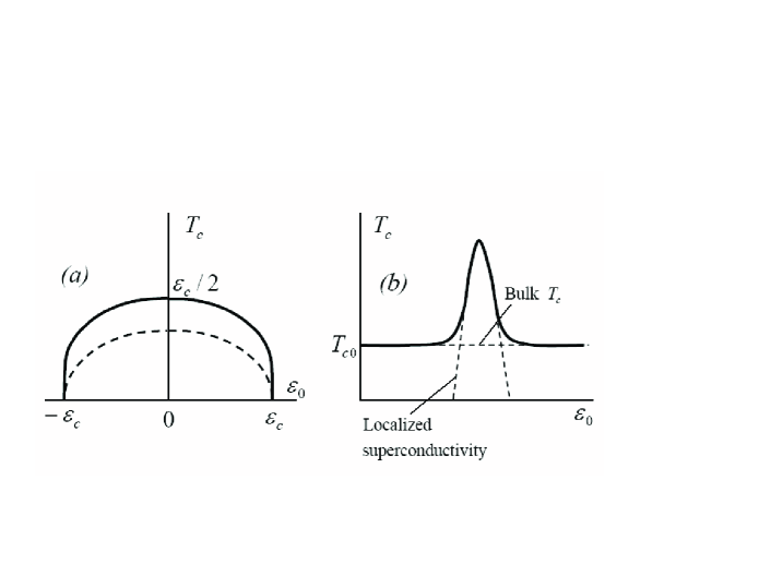
Figure 4: (a) $T_{c}$ of the one-level system as a function of the level position $\epsilon_{0}$ in the absence of attenuation (solid line); attenuation $\gamma$ produces a shift of the curve by the quantity $\sim\gamma$ (dashed line). (b) The same, for a situation when the quasi-discrete level lies in the background of the continuous spectrum.

$$T_{c}=\frac{\epsilon_{0}}{\ln(\epsilon_{c}+\epsilon_{0})-\ln(\epsilon_{c}-\epsilon_{0})}\,,\qquad\epsilon_{c}=gI_{4}/2\,,$$

and a solution exists under condition

$$|\epsilon_{0}|<\epsilon_{c}\,.$$

At first glance, the considered regime is destroyed due to fluctuations  or coupling with the continuous spectrum; in fact, it is not so (see below) and the main problem consists in the possibility to match the discrete level with the Fermi energy.

Indeed, let the system has a finite size $L$, while its eigenstates are extended. Then the Fermi energy is located between two discrete levels , and $\epsilon_{0}$ is determined by the average level spacing $J(L/a)^{-d}$; estimating $I_{4}\sim L^{-d}$ from the normalization condition, we see that

$$\epsilon_{0}\sim J(L/a)^{-d}\,,\qquad\epsilon_{c}\sim gL^{-d}$$

and condition (21) cannot be fulfilled in the weak coupling regime, which is the only allowable in the BCS scheme.

Let us couple the given system with a reservoir, and try to match the chemical potential of the latter with the discrete level of the system. However, nothing good will occur from it: the local Fermi level of the system is still arranged between two discrete levels and it tends to equalize with the Fermi energy in the reservoir. The real flow of electrons is impossible due to elecroneutrality, and the problem will be solved by a minimal deformation: a double layer will arise between the reservoir and the system, and it will equate the Fermi levels.

By the same reason, the situation cannot be improved due to localization of states. At first glance, in this case $\epsilon_{0}\sim J(L/a)^{-d}$, $\epsilon_{c}\sim g\xi^{-d}$ ($\xi$ is the localization radius of $\varphi_{0}(r)$), so condition (21) reduces to $g\mathbin{\lower 3.0pt\hbox{$\hbox to0.0pt{\raise 5.0pt\hbox{$\char 62\relax$}\hss}\mathchar 29208\relax$}}Ja^{d}(L/\xi)^{-d}$ and can be fulfilled at sufficiently large $L$. In fact, blocks of size $\xi$ are quasi-independent and each of them has its own local Fermi level; these levels equalize due to double layers between blocks, and the given estimates are valid only for $L\sim\xi$. In fact, the above arguments clarify the mechanism for the Coulomb gap [25].

It looks that the only possibility to avoid the given arguments is to take the size $L$ of the atomic order. Indeed, at such a scale: (a) the notion of the Fermi level becomes senseless; (b) electroneutrality can be violated; (c) a size of the double layer is comparable with $L$. It means that the strong violations of the Anderson theorem can be exhaustively analyzed by consideration of the one-impurity problem (Sec.4).

Already at this stage it is possible to establish the relation with results of [9, 10]. In the considered there strictly one-electron picture, the discrete system of levels fluctuates freely relative to the Fermi energy, so resonances are possible at any length scale $L$. Then all principal statements of [9, 10] are reproduced: $T_{c}$ has a power law behavior as a function of $g$ and does not depend on the cut-off frequency $\omega_{0}$, while the order parameter $\Delta(r)$ follows the form of the wave function (see (16)) and will have multifractal properties simultaneously with multifractality of the latter.  However, this picture is completely destroyed, if electroneutrality is taken into account, since resonances at large scales become impossible. In fact, large scale fluctuations are insignificant even in a strictly one particle picture: a value of $T_{c}$ for an exact resonance, $T_{c}\sim gL^{-d}$ (see(17),(19)), is greater for small scales.

Generally, the considered regime is not destroyed in the presence of the continuous spectrum. In this case, the level $\epsilon_{0}$ acquires the finite decay $\gamma$, which can be taken into account by replacement

$$\epsilon_{0}\pm i\omega\,\,\longrightarrow\,\,\epsilon_{0}\pm i\omega\pm i\gamma\,{\rm sign}\,\omega$$

so

$$A(T)=T\sum\limits_{\omega}\frac{1}{\epsilon^{2}_{0}+(|\omega|+\gamma)^{2}}\approx$$

$$\approx\frac{1}{\pi\epsilon_{0}}\arctan\frac{\epsilon_{0}}{\gamma+bT}\,,$$

where we have estimated the sum by the integral, introducing the cut-off $|\omega|>bT$ (for the choice $b=4/\pi$ such estimate practically coincides with the exact result (18) for $\gamma=0$). The finiteness of $\gamma$ leads qualitatively to the shift of the curve in Fig.4,a by a quantity $\sim\gamma$, so a solution survives for $\gamma\mathbin{\lower 3.0pt\hbox{$\hbox to0.0pt{\raise 5.0pt\hbox{$\char 60\relax$}\hss}\mathchar 29208\relax$}}\epsilon_{c}$.

For finite $\omega_{0}$ one obtains instead (24)

$$A(T)\approx\frac{1}{\pi\epsilon_{0}}\arctan\frac{\epsilon_{0}(\omega_{0}-bT)}{\epsilon_{0}^{2}+(\omega_{0}+\gamma)(\gamma+bT)}\,,$$

and can be easily convinced that finiteness of $\omega_{0}$ is irrelevant under condition $\omega_{0}\gg\epsilon_{c}$. In the opposite case $\omega_{0}\ll\epsilon_{c}$ the allowed values of $\epsilon_{0}$ and $\gamma$ have an order $(\epsilon_{c}\omega_{0})^{1/2}$, while the maximal critical temperature $T_{c}$ is of the order $\omega_{0}$; in fact, restriction $T_{c}<\omega_{0}/\pi$ is evident, since for $T>\omega_{0}/\pi$ the sum over $\omega$ contains no terms.

To investigate the effect of the continuous spectrum on the order parameter, one can use the following approximation for the kernel $K(r,r^{\prime})$

$$K(r,r^{\prime})=K_{0}(r-r^{\prime})+gA(T)\varphi^{2}_{0}(r)\varphi^{2}_{0}(r^{\prime})\,,$$

which ignores the backward influence of the discrete level on the continuous spectrum. According to [11, 12], such approximation provides qualitatively correct description and can be justified in certain limiting cases. 

Having in mind a consideration of periodical configurations, we solve Eq.4 with the kernel (25) for a finite system of size $L$ with the periodical boundary conditions. We accept $L\ll\xi_{0}\tau^{-1/2}$, where $\tau=(T-T_{c0})/T_{c0}$, $\xi_{0}$ is the coherence length, and $T_{c0}$ is a transition temperature, corresponding to the continuous spectrum.  After the Fourier transform one has

$$\Delta_{q}=gA(T)X\frac{\langle\varphi^{2}_{0}\rangle_{q}}{1-K_{0}(q)}\,,$$

$$X=L^{-d}\sum\limits_{q}\langle\varphi^{2}_{0}\rangle_{-q}\Delta_{q}$$

and self-consistency of two expressions leads to

$$1=gA(T)\left[L^{-d}\sum\limits_{q}\langle\varphi^{2}_{0}\rangle_{q}\langle\varphi^{2}_{0}\rangle_{-q}+\right.$$

$$\left.+L^{-d}\sum\limits_{q}\frac{K_{0}(q)}{1-K_{0}(q)}\langle\varphi^{2}_{0}\rangle_{q}\langle\varphi^{2}_{0}\rangle_{-q}\right]\,.$$

Using expansion in $q^{2}$

$$1-K_{0}(q)=\lambda_{0}\tau+{\scriptstyle\frac{1}{2}}\lambda_{0}\xi_{0}^{2}q^{2}+\ldots\,,$$

it is easy to see that the main contribution to the second sum in (27) occurs from small $q$, and the single term with $q=0$ is sufficient for $L\ll\xi_{0}\tau^{-1/2}$. Then Eq.27 accepts a form

$$1=gA(T)\left[I_{4}+\frac{1}{\lambda_{0}L^{d}\tau}\right]\,,$$

and the analogous approximations in (26) give

$$\Delta(r)=const\left[\varphi_{0}^{2}(r)+\frac{1}{\lambda_{0}L^{d}\tau}\right]\,.$$

If $T_{c0}\ll\epsilon_{c}$, then dependence of $T_{c}$ on $\epsilon_{0}$ has a form shown in Fig.4,b. In the zero approximation there are two independent systems, the quasi-local one with the transition temperature (20) (if attenuation $\gamma$ is small) and the continuous one characterizing by $T_{c0}$, while $T_{c}$ of the composed system is given by the maximal of two values. Interrelation of two systems reduces to smoothing of dependence $T_{c}(\epsilon_{0})$ at the scale $T_{c0}(a/L)^{d/2}$, if $\varphi(r)$ is localized at the atomic scale $a$.

It is clear from (30) that the order parameter $\Delta(r)$ is practically constant for small $\tau$ and localized at the scale $a$ for large $\tau$. Crossover from one regime to another is very abrupt, and one can say on the ”Anderson transition” for superconducting electrons. We see that the localized regime survives in the presence of the continuous spectrum, if the corresponding $T_{c}$ exceeds $T_{c0}$. In fact, existence of the continuous spectrum has a stabilizing effect on the localized superconductivity, since the order parameter takes non-zero values in the whole volume.

4. One-impurity problem

If $G^{0}_{nn^{\prime}}$ is the Green function of an ideal lattice, $V_{n}=V\delta_{nn_{0}}$ is an impurity potential, then the Green function $G_{nn^{\prime}}$ of the perturbed system is determined by the Dyson equation [26]:

$$G_{nn^{\prime}}=G^{0}_{nn^{\prime}}+G^{0}_{nn_{0}}VG_{n_{0}n^{\prime}}\,.$$

Setting $n=n_{0}$, one has the closed equation for $G_{n_{0}n^{\prime}}$, whose solution is substituted into (31)

$$G_{nn^{\prime}}=G^{0}_{nn^{\prime}}+G^{0}_{nn_{0}}{\cal T}G^{0}_{n_{0}n^{\prime}}\,,\qquad$$

$${\cal T}=\frac{V}{1-VG^{0}_{n_{0}n_{0}}}\,,$$

where the scattering ${\cal T}$-matrix reduces to a constant in the given case. For an ideal lattice $G^{0}_{nn}$ does not depend on $n$,

$$G^{0}_{nn}=\int\frac{d^{d}k}{(2\pi)^{d}}\frac{1}{E-\epsilon_{k}+i0}=$$

$$=\int\frac{\nu_{0}(\epsilon)\,d\epsilon}{E-\epsilon+i0}\equiv I(E)-i\pi\nu_{0}(E)\,$$

and so ${\cal T}$-matrix has no $n_{0}$ dependence. Condition $1-VI(E)=0$ corresponds to existence of the local (if $\nu_{0}(E)=0$) or quasi-local (if $\nu_{0}(E)\neq 0$) level [26, 27] (Fig.5). The local density at site $n_{0}$

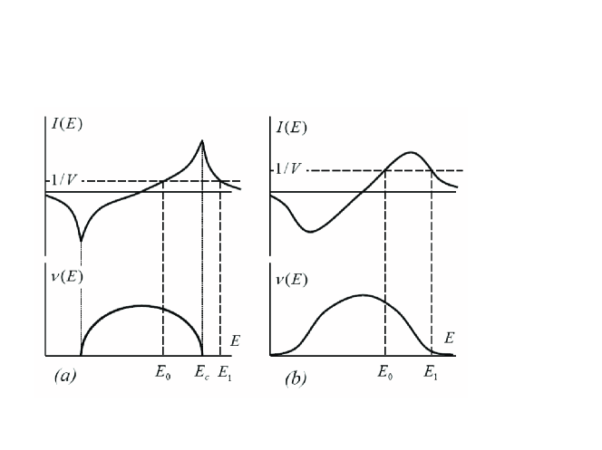
Figure 5: (a) If the impurity $V\delta_{nn_{0}}$ is inserted in an ideal lattice, equation $1=VI(E)$ has two roots for large $V$, $E_{1}$ and $E_{0}$, which correspond to the local and quasi-local levels. (b) If the same impurity is inserted in the disordered lattice, both solutions correspond to the quasi-local levels.

$$\nu(E,{n_{0}})=\frac{\nu_{0}(E)}{[1-VI(E)]^{2}+[\pi V\nu_{0}(E)]^{2}}$$

has an abrupt maximum near the resonance $1-VI(\epsilon_{0})=0$ (Fig.6) with a value in it

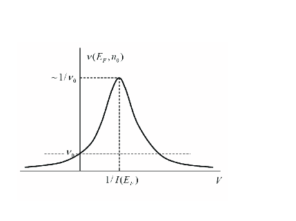
Figure 6: The local density of states at the point $n_{0}$ as a function of the impurity potential $V$.

$$\left[\nu(E,{n_{0}})\right]_{res}=\frac{I(\epsilon_{0})^{2}}{\pi^{2}\nu_{0}(\epsilon_{0})}$$

which grows unboundedly near the initial band edge (where $\nu_{0}(\epsilon_{0})\to 0$). In the vicinity of the band edge, a calculation of $G^{0}_{nn^{\prime}}$ is possible in the continual approximation and gives at $d=3$ (for $|r-r^{\prime}|\mathbin{\lower 3.0pt\hbox{$\hbox to0.0pt{\raise 5.0pt\hbox{$\char 62\relax$}\hss}\mathchar 29208\relax$}}a$ ):

$$G^{0}_{nn^{\prime}}\,\longrightarrow\,G^{0}(r-r^{\prime})=-\pi\nu_{0}\,\frac{e^{ik_{F}|r-r^{\prime}|}}{k_{F}|r-r^{\prime}|}\,,$$

Deviation of $\nu(E,{n_{0}})$ from $\nu_{0}(E)$ is maximal for $n=n_{0}$ and tends to zero for $|n-n^{\prime}|\to\infty$.

The Matsubara representation for the Green functions is obtained from (32) by replacement $E\to\epsilon_{F}+i\omega$, where $\epsilon_{F}=0$ for the corresponding choice of the energy origin. Setting $n_{0}=0$, one has for the kernel in (4)

$$K(r,r^{\prime})=gT\sum_{\omega}\left|G_{\omega}(r,r^{\prime})\right|^{2}=$$

$$=gT\sum_{\omega}\left|G^{0}_{\omega}(r-r^{\prime})\right|^{2}+\qquad\qquad\qquad$$

$$\quad+gT\sum\limits_{\omega}\,G^{0}_{\omega}(r)\,{\cal T}_{\omega}\,G^{0}_{\omega}(r^{\prime})\,G^{0}_{-\omega}(r-r^{\prime})+$$

$$\qquad+gT\sum\limits_{\omega}\,G^{0}_{-\omega}(r)\,\,{\cal T}_{-\omega}\,G^{0}_{-\omega}(r^{\prime})\,G^{0}_{\omega}(r-r^{\prime})+$$

$$+gT\sum\limits_{\omega}\,\left|G^{0}_{\omega}(r)\right|^{2}\,\left|{\cal T}_{\omega}\right|^{2}\,\left|G^{0}_{\omega}(r^{\prime})\right|^{2}\equiv\quad$$

$$\equiv K_{0}(r-r^{\prime})+K_{1}(r,r^{\prime})\,.$$

Solution of the Gor’kov equation with the kernel (37) is sought in the form

$$\Delta(r)=\Delta_{0}+\Delta_{1}(r)\,,$$

where $\Delta_{1}(r)$ is localized near $r=0$. Substituting in (4) and using the sum rule (7), one has

$$\Delta(r)=\int K_{0}(r-r^{\prime})\Delta(r^{\prime})d^{3}r^{\prime}+$$

$$+g\nu_{1}(r)\ln\frac{1.14\omega_{0}}{T}\Delta_{0}+F(r)\,$$

where $\nu_{1}(r)$ is deviation of the local density of states from $\nu_{0}$ and

$$F(r)=\int K_{1}(r,r^{\prime})\Delta_{1}(r^{\prime})d^{3}r^{\prime}\,.$$

Consideration of the isolated impurities is not actual (see Footnote 6), so we accept their periodical arrangement and solve the Gor’kov equation for a finite system of size $L$ with periodical boundary conditions for $L\ll\xi_{0}\tau^{-1/2}$. Resolving (39) for $\Delta(r)$ by the Fourier transform and and simplifying the result analogously to (27), it is possible to separate the uniform term corresponding to $\Delta_{0}$, while the rest is attributed to $\Delta_{1}(r)$ ($\langle\ldots\rangle_{0}$ is the zero Fourier component):

$$\Delta_{0}=\frac{K_{0}(0)}{\lambda_{0}L^{3}\tau}\left[\,\Delta_{0}\ln\frac{1.14\omega_{0}}{T}\,g\langle\nu_{1}\rangle_{0}+\langle F\rangle_{0}\,\right]\,,$$

$$\Delta_{1}(r)=\Delta_{0}\,\ln\frac{1.14\omega_{0}}{T}\,g\nu_{1}(r)+\,F(r)\,.$$

Using the explicit expression for $F(r)$ and setting in the integrals 

$$\Delta_{1}(r^{\prime})G^{0}_{\omega}(r-r^{\prime})\approx\Delta_{1}(r^{\prime})G^{0}_{\omega}(r)\,,$$

one can transform (41) to the form

$$\Delta_{0}=\frac{K_{0}(0)}{\lambda_{0}L^{3}\tau}\,\ln\frac{1.14\omega_{0}}{T}\,\left[\vphantom{A^{2}_{6}}\,g\langle\nu_{1}\rangle_{0}\,\Delta_{0}\,+\,g\langle\nu_{1}\Delta_{1}\rangle_{0}\,\right]\,,$$

$$\Delta_{1}(r)=\Delta_{0}\,\ln\frac{1.14\omega_{0}}{T}\,g\nu_{1}(r)+\,gT\sum\limits_{\omega}\,Z_{\omega}\,|G^{0}_{\omega}(r)|^{2}\,.$$

where

$$Z_{\omega}=\,{\cal T}_{\omega}\,Y_{\omega}\,+\,{\cal T}_{-\omega}\,Y_{-\omega}\,+\left|{\cal T}_{\omega}\right|^{2}\,X_{\omega}\,,$$

$$\qquad X_{\omega}=\int\,\Delta_{1}(r)\,\left|G^{0}_{\omega}(r)\right|^{2}\,d^{3}r\,,\,$$

$$Y_{\omega}=\int\,\Delta_{1}(r)\,G^{0}_{\omega}(r)\,d^{3}r\,.$$

Substituting $\Delta_{1}(r)$ from (43$b$) into expressions (44), and estimating arising integrals

$$g\int\nu_{1}(r)\,|G^{0}_{\omega}(r)|^{2}\,d^{3}r\equiv\lambda_{01}\,,\qquad$$

$$g\int|G^{0}_{\omega}(r)|^{2}|G^{0}_{\omega^{\prime}}(r)|^{2}\,d^{3}r\equiv\lambda_{11}\,,\qquad$$

$$g\int\nu_{1}(r)\,G^{0}_{\omega}(r)\,d^{3}r\equiv\lambda^{\prime}_{02}+i\lambda^{\prime\prime}_{02}\,{\rm sign}\,\omega\,,\qquad$$

$$g\int G^{0}_{\omega}(r)\,|G^{0}_{\omega^{\prime}}(r)|^{2}\,d^{3}r\equiv\lambda^{\prime}_{12}+i\lambda^{\prime\prime}_{12}\,{\rm sign}\,\omega\,$$

with the use of expressions for $G^{0}_{\omega}(r)$ and $\nu_{1}(r)$ (where the real and imaginary parts are denoted by a prime and two primes)

$$G^{0}_{\omega}(r)=-\frac{\pi\nu_{0}}{k_{F}r}\exp\left\{-\frac{|\omega|}{v_{F}}r+ik_{F}r\,{\rm sign}\,\omega\right\}$$

$$\nu_{1}(r)=-\pi\nu_{0}^{2}\,\frac{{\cal T}^{\prime\prime}\cos{2k_{F}r}+{\cal T}^{\prime}\sin{2k_{F}r}}{(k_{F}r)^{2}}\,,$$

it is easy to see that the integrals converge already for $\omega,\,\,\omega^{\prime}=0$, so parameters $\lambda_{01}$, $\lambda_{11}$, etc. can be considered as constant; it allows to write (44) in the form

$$X_{\omega}=X\,,\qquad Y_{\omega}=Y^{\prime}+iY^{\prime\prime}\,{\rm sign}\,\omega\,,$$

$$Z_{\omega}=2\,{\cal T}^{\prime}_{\omega}\,Y^{\prime}\,-2\,|{\cal T}^{\prime\prime}_{\omega}|\,Y^{\prime\prime}\,+\left|{\cal T}_{\omega}\right|^{2}\,X\,.$$

The region remote from the resonance. The natural scale for the energy dependence of ${\cal T}$-matrix is given by the bandwidth $J$, so ${\cal T}^{\prime}_{\omega}$ and $|{\cal T}^{\prime\prime}_{\omega}|$ can be considered as independent of $\omega$ anywhere, excepting the vicinity of the resonance (see below). Then $Z_{\omega}$ is also independent of $\omega$, and substitution of $\Delta_{1}(r)$ from (43$b$) into (44) leads to the linear system of equations for $\Delta_{0}$ and $Z$ (see Appendix), whose solubility condition gives

$$\frac{\delta T_{c}}{T_{c0}}=\frac{1}{\lambda_{0}L^{3}}\,\int d^{3}r\,\frac{\nu_{0}\nu_{1}(r)+\nu_{1}(r)^{2}}{\nu_{0}^{2}}\,.$$

Eq. 48 is a natural generalization of the result (1): the first term in the numerator corresponds to the Anderson theorem, while the second determines corrections to it. A configuration of the order parameter shows that (48) corresponds to the delocalized regime.

For weak impurities ($|V|\ll J$) one has the estimates

$${\cal T}^{\prime}\approx{\cal T}\sim Va^{3}\,,\qquad{\cal T}^{\prime\prime}\sim Va^{3}(V/J)(k_{F}a)\,,$$

and

$$\nu_{0}\langle\nu_{1}\rangle_{0}\sim a^{3}\nu_{0}^{2}\,(V/J)(k_{F}a)^{-2}\,,$$

$$\langle\nu_{1}^{2}\rangle_{0}\sim a^{3}\nu_{0}^{2}\,(V^{2}/J^{2})(k_{F}a)^{-1}\,,$$

so the Anderson term is leading both in parameter $V/J$ and in parameter $(k_{F}a)^{-1}$. We accepted here $k_{F}a\ll 1$, having in mind a situation near the band end, while estimates for the band center follow at $k_{F}a\sim 1$.

The delocalized regime retains in the case when the resonance condition $1\approx VI(\epsilon_{F})$ is formally fulfilled, but the density of states $\nu(\epsilon_{F})$ is sufficiently large to provide a strong attenuation of the quasi-local state. In this situation

$${\cal T}^{\prime}\sim Ja^{3}\frac{J\epsilon_{0}}{\gamma^{2}}\,,\qquad{\cal T}^{\prime\prime}\sim Ja^{3}\frac{J}{\gamma}\,,$$

and one has under condition $\gamma\mathbin{\lower 3.0pt\hbox{$\hbox to0.0pt{\raise 5.0pt\hbox{$\char 62\relax$}\hss}\mathchar 29208\relax$}}\epsilon_{0}$ (where $\epsilon_{0}$ and $\gamma$ are defined in Eq. 54)

$$\nu_{0}\,\langle\nu_{1}\rangle_{0}\sim\langle\nu_{1}^{2}\rangle_{0}\sim a^{3}\nu_{0}^{2}\,(k_{F}a)^{-2}\,,$$

i.e. the Anderson term has the same order, as a correction to it.

Vicinity of the resonance. If $\epsilon_{0}$ is a root of equation $1=VI(\epsilon)$, then in the vicinity of it

$$1-VI(\epsilon)=(\epsilon-\epsilon_{0})/E_{0}\,,\qquad E_{0}\sim J\,,$$

and hence

$${\cal T}=\frac{VE_{0}}{\epsilon-\epsilon_{0}+i\gamma}\,,\qquad\gamma=\pi VE_{0}\nu(\epsilon_{0})\,.$$

In the Matsubara representation one has

$${\cal T}_{\omega}=\frac{VE_{0}}{i\omega-\epsilon_{0}+i\gamma\,{\rm sign}\,\omega}\,\equiv{\cal T}^{\prime}_{\omega}-i|{\cal T}^{\prime\prime}_{\omega}|{\rm sign}\,\omega\,,$$

where

$${\cal T}^{\prime}_{\omega}=-VE_{0}\,\frac{\epsilon_{0}}{\epsilon^{2}_{0}+(|\omega|+\gamma)^{2}}\,,$$

$$\qquad\qquad|{\cal T}^{\prime\prime}_{\omega}|=VE_{0}\,\frac{|\omega|+\gamma}{\epsilon^{2}_{0}+(|\omega|+\gamma)^{2}}\,,$$

so ${\cal T}$-matrix can be considered as independent of $\omega$ under condition

$$|\omega|\ll\gamma\,,\qquad{\rm or}\qquad k_{F}a\gg\omega/J\,,$$

i.e. not very close to the initial band edge. If this condition is not fulfilled , then the $\omega$ dependence is essential for the quantities ${\cal T}^{\prime}_{\omega}$ and $|{\cal T}^{\prime\prime}_{\omega}|$, and hence for $Z_{\omega}$. In fact, only one combination is relevant,

$$S=T\sum\limits_{\omega}\,Z_{\omega}\,,\qquad$$

and substitution of $\Delta_{1}(r)$ from (43$b$) into (44) allows to express $Z_{\omega}$ through $\Delta_{0}$ and $S$; substituting this expression for $Z_{\omega}$ into (58) and (43), one comes to the linear system of equations for $\Delta_{0}$ and $S$; its solubility condition with only leading terms retained (see Appendix) reduces to

$$\left(\tau-\frac{\nu_{0}\langle\nu_{1}\rangle_{0}\!+\!\langle\nu_{1}^{2}\rangle_{0}}{\lambda_{0}L^{3}\,\nu_{0}^{2}}\right)\left(-1+\lambda_{11}V^{2}E_{0}^{2}A(T)\right)+$$

$$\qquad+\,\tau_{c}^{2}=0\,,$$

where $A(T)$ corresponds to expression (24). Equation (59) describes the typical situation related with intersection of terms. The zero of the first bracket corresponds to the delocalized regime (see Eq.48), and vanishing of the second bracket corresponds to equation for $T_{c}$ of the localized superconductivity (compare with (17, 24)), while the term $\tau_{c}^{2}\sim(a/L)^{3}$ removes the degeneracy of terms in the intersection point (Fig.7).

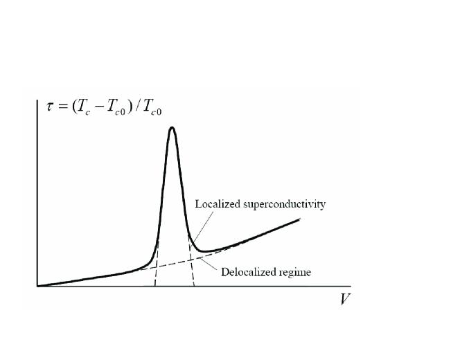
Figure 7: Dependence of $T_{c}$ on the impurity potential $V$ for a small impurity concentration.

5. Consequences for the Anderson model.

Usually localization is studied in the framework of the Anderson model, which is a discrete version of the Schroedinger equation with a random potential: the bare spectrum is a band of width $J$, while the potential values $V_{n}$ on the lattice sites are independent random quantities with the distribution $P\{V\}$ of width $\sim W$, which is supposed to be rectangular. To transfer from the one-impurity problem to the Anderson model, it is sufficient to accept that a potential $V$ of impurities fluctuates in the interval $(-W,W)$, while their concentration $c$ is gradually increased from small values to values of the order of unity.

The results of Sec.4 correspond formally to the periodic arrangement of impurities, but in fact their periodicity is not essential: each impurity arouses only a local deformation of the order parameter and these deformations are independent in case of a small concentration. If $\Delta_{1}(r)$ and $\nu_{1}(r)$ correspond to the one-impurity problem, then configurations

$$\Delta(r)=\Delta_{0}+\sum\limits_{i}\Delta_{1}(r-r_{i})\,,$$

$$\nu_{F}(r)=\nu_{0}+\sum\limits_{i}\nu_{1}(r-r_{i})\,$$

correspond to a situation, when several impurities are arranged in points $r_{i}$: it is a consequence of localization of the kernel $K_{1}(r,r^{\prime})$ in both variables near the defect position. It is clear from (41) that the amplitude of $\Delta_{1}(r)$ is proportional to $\Delta_{0}$, so $\Delta_{1}(r)=\Delta_{0}f(r)$ and substitution of (60) into (10) gives for $T_{c}$ close to $T_{c0}$:

$$\frac{\delta T_{c}}{T_{c0}}=\frac{m}{\lambda_{0}^{2}L^{3}}\,g\!\int d^{3}r\left[\nu_{1}(r)+\nu_{1}(r)f(r)\right]\,.$$

Here $m$ is a number of impurities in the volume $L^{3}$, and $f(r)$ can be identified as $\nu_{1}(r)/\nu_{0}$ from comparison with (48) . One can see that effect is proportional to a concentration of impurities, while their arrangement is irrelevant. The Anderson theorem is valid under condition $|f(r)|\ll 1$, which is fulfilled for weak impurities. In case of nonequivalent impurities, the result (61) should be averaged according to distribution $P(V)$.

In the regime of the localized order parameter, each impurity is practically independent of enviroment and $T_{c}$ of the system is determined by those of them, which are close to a resonance; if distribution $P(V)$ is continuous and sufficiently wide, then the condition of almost exact resonance is always realized with a certain probability. Therefore, the concentration of the resonant impurities is finite and their quasiperiodic arrangement stabilizes the mean-field solution.

Above considerations completely clarify a situation for small impurity concentrations. Advancement to higher concentrations is simplified by observation that equations (31), (32) never used a fact that $G^{0}_{nn^{\prime}}$ corresponds to an ideal lattice; the same equations describe insertion of an additional impurity in the disordered superconductor. Noticing that

$$G^{0}_{n_{0}n_{0}}=\sum\limits_{s}\frac{|\varphi_{s}(n_{0})|^{2}}{E-\epsilon_{s}+i0}=\int\limits d\epsilon\frac{\nu(\epsilon,n_{0})}{E-\epsilon+i0}$$

and replacing $\nu(\epsilon,n_{0})$ by its mean value $\langle\nu(\epsilon)\rangle$, we obtain the same representation $I(E)-i\pi\nu(E)$ as in Eq.33, with a predictable behavior of $I(E)$ and $\nu(E)$ (Fig.5,$b$).

Weak impurities. In this case, a behavior of functions $I(E)$ and $\nu(E)$ differs from their behavior in an ideal crystal by small smoothening of the Van Hove singularities (Fig.5,$b$). Dependence on $n_{0}$ results in fluctuations of the form of these functions, which are also small. It is clear that for weak impurities ($|V|\ll J$) the resonance condition is not fulfilled and no localization of the order parameter is possible.

For the delocalized regime, it is convenient to present the result (61) in another form. Taking the one-impurity configuration $\Delta(r)=\Delta_{0}+\Delta_{0}f(r)$, $\nu(r)=\nu_{0}+\nu_{1}(r)$ and substituting it into equation (10), we have for the effective density of states entering into the BCS formula:

$$\nu_{eff}=\frac{\nu_{0}+\nu_{0}\langle f\rangle+\langle\nu_{1}\rangle+\langle\nu_{1}f\rangle}{1+\langle f\rangle}\,.$$

Subtracting the result with $f\equiv 0$ and retaining the main terms in $L^{-d}$:

$$\nu_{eff}-\langle\nu\rangle\,=\,\langle\nu_{1}f\rangle\,=\,\frac{\langle\nu^{2}_{1}f\rangle}{\nu_{0}}\,=\,\frac{\,\,\nu_{0}\left({\cal T}^{\prime}\right)^{2}}{4k_{F}L^{3}}\,,$$

$$\langle\nu\rangle-\nu_{0}\,=\,\langle\nu_{1}\rangle\,=\,-\,\frac{(\nu_{0}{\cal T}^{\prime})}{2k_{F}^{2}L^{3}}\,,$$

where we have taken into account that only the term with ${\cal T}^{\prime}\approx V+V^{2}I(E_{F})$ is essential in Eq.46 for weak impurities. Inserting impurities one after another and averaging over $V$,

$$\nu_{eff}-\langle\nu\rangle\sim c\nu_{0}\,\frac{W^{2}}{J^{2}}\,(k_{F}a)^{-1}\,,$$

$$\langle\nu\rangle-\nu_{0}\sim c\nu_{0}\,\frac{W^{2}}{J^{2}}\,(k_{F}a)^{-2}\,,\,\,$$

we see that in the course of increasing a concentration, the increment of the quantity $\nu_{eff}-\langle\nu\rangle$ is by a factor $k_{F}a$ smaller than the increment of $\langle\nu\rangle-\nu_{0}$. Near the band edge one have $\langle\nu\rangle\gg\nu_{0}$ for sufficiently large concentrations, so $\nu_{eff}-\langle\nu\rangle\sim k_{F}a\langle\nu\rangle$ and deviations from the Anderson theorem are small. Near the band center we have $k_{F}a\sim 1$ and differencies $\langle\nu\rangle-\nu_{0}$ and $\nu_{eff}-\langle\nu\rangle$ are small till concentrations $c\sim 1$; so $\nu_{eff}-\langle\nu\rangle\ll\langle\nu\rangle$. It is clear that violation of self-averaging for the order parameter does not occur for weak impurities.

In the $3D$ case, isolated weak impurities do not produce bound states beyond the initial spectrum (it is clear from Fig.5,$a$), and a finite density of states in this energy interval is a collective phenomenon related with long-range fluctuations of the band edge. Consider a fluctuation in the region of size $L$, due to which the range of $V$ values is somewhat restricted, $(-W,W-2\delta)$ instead $(-W,W)$. Then the mean value of the random potential is decreased by a quantity $\delta$, while a probability of such fluctuation

$\exp(-L^{d}\delta/W)$ is not small for $L^{d}\delta/W\mathbin{\lower 3.0pt\hbox{$\hbox to0.0pt{\raise 5.0pt\hbox{$\char 60\relax$}\hss}\mathchar 29208\relax$}}1$. Such fluctuations occur at all scales and produce a finite density of states beyond the bare spectrum.  If size $L$ of the fluctuation is sufficient for existing of superconductivity, the latter will not differ from superconductivity in the initial system with not shifted band edge; i.e. impurities will not violate the uniformity of the order parameter. Near the initial band edge, the indicated fluctuations strongly overlap and superconductivity is quasi-homogeneous. Such fluctuations become spatially isolated in the region of strong localization, where they can be described in terms of the size effect (Sec.6).

Strong impurities. For a small concentration of strong impurities ($|V|\mathbin{\lower 3.0pt\hbox{$\hbox to0.0pt{\raise 5.0pt\hbox{$\char 62\relax$}\hss}\mathchar 29208\relax$}}J$), a behavior of functions $I(E)$ and $\nu(E)$ is not very different from their behavior in an ideal crystal. However, in the region of the maximum of $I(E)$ the density of states becomes finite and, at first glance, complicates the occurrence of resonances. In fact, a new phenomenon comes to life. Since now $G^{0}_{n_{0}n_{0}}$ depends on $n_{0}$, the attenuation of the quasi-local state will be determined not by average density of states, but its local value at the point $n_{0}$, which can be small in a fluctuational manner. As a result, resonances become possible even for energies in the deep of the band, where they were forbidden in the ideal lattice. The typical situation, when the local density of states $\nu_{F}(n_{0})$ is small, corresponds to large values of the random potential in the vicinity of $n_{0}$; if now an impurity with large negative $V$ is inserted into the site $n_{0}$, then a specific

Figure 8: A typical fluctuation of the random potential responsible for existence of the quasi-local state in the deep of the allowed band.

resonance configuration arises (Fig.8).  In the ”minimal” variant, such configuration corresponds to existence of large barriers at the nearest neighbours of site $n_{0}$, while a value of the potential at $n_{0}$ is chosen so that a corresponding level was in the interval of width $\sim T_{c}$ near the Fermi energy (the probability of this event is $\sim T_{c}/W$). For a finite band, both large positive and large negative value of the potential are locking, and for $W\gg J$ such values occur with probability $p$ close to unity. Therefore, the probability of the ”minimal” fluctuation

$$P_{res}\sim p^{Z}\frac{T_{c}}{W}\,,$$

where $Z$ is a number of the nearest neighbours. It is clear that such resonances can occur for any position of the Fermi level. In the region of the fluctuational tail, the density of states is small by the natural reasons and there is no need to create the barrier around $n_{0}$; so the factor $p^{Z}$ will be absent but the less probable form of the effective potential well is necessary, in order the level was in the desired part of the spectrum.  With increasing of the impurity concentration, the effective bandwidth is extended and the maximum of $I(E)$ is shifted correspondingly. However, the general mechanism of resonances and estimation of their probability remain unchanged.

Since the true critical temperature is hardly observable, it is actual to consider the ”bulk $T_{c}$”, which can be defined as $T_{c}$ of the system with excluded resonant impurities. For strong but not resonant impurities, two terms in Eq.48 are of the same order (see (50, 52)), and impurities are independent till concentrations $c\sim 1$, since the mobility edge lies far from the bare edge of spectrum and $k_{F}a\sim 1$. Validity of the Anderson theorem holds on the qualitative level: $T_{c}$ is determined by the effective density of states, which differs from the average one by a factor of the order of unity.

6. Size effect in the localized phase.

In the localized phase, the system breaks up into quasi-independent blocks of size $\xi$, and superconductivity is suppressed due to the size effect. Below we analyze this effect in terms of the Gor’kov equation. Superconductivity in small samples was discussed in many papers (see a review article [29]), but this discussion mainly concerns the aspects:

(a) inadequacy of the grand canonical ensemble due to a fixed number of electrons in small granules;

(b) parity effects;

(c) insufficiency of the mean field approximation;

(d) absence of an abrupt phase transition, etc.

which are essential for finite systems and completely not actual in the present context. In principle, it is correct to stress unreliebility of the mean field approach, but all attempts to overcome it (from modified mean field approximations till the exact Richardson solution and a direct numerical modelling) are based on the truncated BCS Hamiltonian, which by itself induces the certain way of pairing (in general incorrect) . As for the Gor’kov equation, it corresponds to the saddle-point approximation in the functional integral [30, 31] and is the most grounded of all mean-field type approaches; in addition, the electron interaction is specified in the physically clear manner and independently of one-electron states (Sec.2). The accuracy of approximation is determined by the Ginzburg parameter, which provides insignificance of fluctuations in case of a superconductor (with exception of some special cases: e.g. in finite systems fluctuations have a qualitative importance, destroying a phase transition). The Gor’kov equation can be also obtained from the Eliashberg equations in the limit of the local interaction [14].

Consider the cubic sample of size $L$, accepting the periodical boundary conditions for the electron eigenfunctions. In a pure superconductor the latter have a form of plain waves, so $|\varphi_{s}(r)|^{2}=L^{-d}$ and the local density of states (8) does not depend on $r$. Then $\Delta(r)=const$ is an exact solution of the Gor’kov equation (4), which reduces to

$$\Delta=gT\sum\limits_{\omega}L^{-d}\sum\limits_{s}\frac{1}{\epsilon_{s}^{2}+\omega^{2}}\Delta$$

and coincides with (9) in case of the continuous spectrum. In a small energy interval, the spectrum can be considered as a set of equidistant levels with a spacing $\Omega$

$$\epsilon_{s}=\Omega(s+1/2)\,,\qquad\Omega=1/\nu_{F}L^{d}\,,$$

where we accept that the Fermi energy lies in the middle between two discrete levels . Substitution to (66) and summation over $s$ gives

$$1=gT\sum\limits_{\omega}\frac{\pi\nu_{F}}{|\omega|}\tanh\frac{\pi|\omega|}{\Omega}\,.$$

For small $\Omega$, the argument of the hyperbolic tangent is large and one can set $\tanh{x}=1-2e^{-2x}$, so

$$\frac{1}{g\nu_{F}}=\ln\frac{1.14\omega_{0}}{T}-4e^{-2\pi^{2}T/\Omega}\,,$$

where we retained only main terms with $\omega=\pm\pi T$ in the second sum over $\omega$. Subtracting the analogous equation with $\Omega=0$, it is easy to obtain

$$T_{c}=T_{c0}\left[1-4e^{-2\pi^{2}T_{c0}/\Omega}\right]\,,\qquad\Omega\ll T_{c0}\,.$$

For $T\to 0$, one can replace summation in (68) by integration and obtain the equation for the critical value of $\Omega$, at which superconductivity is destroyed

$$\frac{1}{g\nu_{F}}=\int_{-\omega_{0}}^{\omega_{0}}\frac{d\omega}{2\omega}\tanh\frac{\pi\omega}{\Omega_{c}}=$$

$$=\ln\frac{\pi\omega_{0}}{\Omega_{c}}-\int_{0}^{\infty}\frac{\ln x}{\cosh^{2}x}dx\,.$$

The last integral is equal $\ln(\pi/4\gamma)$, where $\ln\gamma=C=0.577$ is the Euler constant and comparing with the result for $T_{c0}$

$$1=g\nu_{F}\ln\frac{4\gamma\omega_{0}}{\Omega_{c}}\,,\qquad 1=g\nu_{F}\ln\frac{2\gamma\omega_{0}}{\pi T_{c0}}\,,$$

one can see that

$$\Omega_{c}=2\pi T_{c0}\,.$$

To find the dependence of $T_{c}$ on $\Omega$ in the vicinity of $\Omega_{c}$, one can transfer (68) using the Poisson summation formula [32]

$$\frac{1}{g\nu_{F}}=\sum\limits_{s=-\infty}^{\infty}e^{-i\pi s}\int\limits_{-\pi\omega_{0}/\Omega}^{\pi\omega_{0}/\Omega}dx\,\frac{\tanh x}{2x}\exp\left\{i\frac{s\Omega}{\pi T}x\right\}\,,$$

where the term with $s=0$ corresponds to (71). For $s\neq 0$, the integrals are convergent at large $|x|$ and it is possible to set $\omega_{0}=\infty$ in them. Due to evenness in $s$ they can be calculated for $s>0$; then the contour is shifted in the upper half-plain and the main contribution arises from the pole $x=i\pi/2$. For $\Omega/T\gg 1$ it is sufficient to retain the terms with $s=0,\pm 1$,

$$\frac{1}{g\nu_{F}}=\ln\frac{4\gamma\omega_{0}}{\Omega}-4e^{-\Omega/2T}\,,$$

and subtracting the analogous equation with $T=0$

$$T_{c}=\frac{\Omega_{c}}{2\ln\left[4\Omega_{c}/(\Omega_{c}-\Omega)\right]}\,,\qquad\Omega\to\Omega_{c}$$

In the reduced coordinates

$$y=T_{c}/T_{c0}\,,\qquad x=\Omega/\Omega_{c}$$

one can obtain the universal dependence $y(x)$. Indeed, transforming (68) by subtraction of the analogous equation with $\Omega=0$, one has

$$\ln\frac{T}{T_{c0}}=T\sum\limits_{\omega}\frac{\pi}{|\omega|}\left(\tanh\frac{\pi|\omega|}{\Omega}-1\right)\,,$$

where $\omega_{0}$ can be set to infinity. Substituting the Matsubara values $\pi T(2n+1)$ for $\omega$, one can present the dependence $y(x)$ in the parametric form

$$y=\exp F(t)\,,\qquad x=t^{-1}\exp F(t)\,,$$

$$F(t)=2\sum\limits_{n=0}^{\infty}\frac{1}{2n+1}\left[\tanh\frac{\pi(2n+1)t}{2}-1\right]\,,$$

where $t$ runs from zero to infinity. Numerical calculation based on (79) gives the ”rectangular” dependence $y(x)$ shown in Fig.9: this dependence has exponentially small deviation from the horizontal line near $y=1$, and exponentially small deviation from the vertical line near $x=1$.

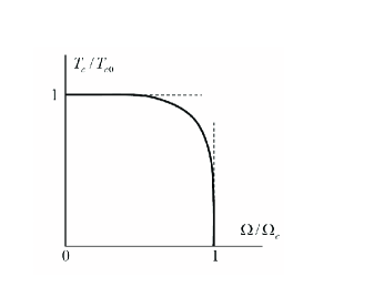
Figure 9: ”Rectangular” dependence of $T_{c}$ on the level spacing $\Omega$ in a finite system; it is universal in the reduced coordinates $y=T_{c}/T_{c0}$, $x=\Omega/\Omega_{c}$.

The given consideration retains for a disordered superconductor if possibility of self-averaging is accepted. . The obtained results can be used to describe the dependence of $T_{c}$ on the distance to the mobility edge in the localized phase, where the system is divided into quasi-independent blocks of size $\xi$. The role of $\Omega$ is played by the quantity

$$\Omega(E)\sim J(\xi/a)^{-d}\sim J(|E-E_{c}|/J)^{d\nu}\,,$$

where $\nu$ is the critical exponent of the localization length. According to Sec.5, the assumption of self-averaging is valid literally for weak disorder and on the qualitative level for strong disorder in the absence of resonances. In the latter case, $T_{c}$ is determined by the effective density of states which differs from the average one by a factor of the order of unity, which is a smooth function of parameters. It preserves the character of singularities (70) and (76), which determine the behavior near $E_{c}$ and $E^{*}$ (Fig.3) and are responsible for the most striking features in the dependence $T_{c}(\epsilon_{F})$.

7. Conclusion.

The present paper resolves contradiction between two series of papers [1]–[5] and [9, 10]. The obtained results has in some way a compromise character. On the one hand, the ”bulk” superconductivity behaves in correspondence with the picture by Bulaevskii and Sadovskii [1]–[5]. On the other hand, the true transition temperature $T_{c}$ of strongly disordered superconductor does not coincide with the ”bulk” one and is determined by rare peaks of the order parameter on the atomic scale; in correspondence with [9, 10] it has a power law dependence on the coupling constant and does not depend on the cut-off frequency. However, in contrast to [9, 10], it has no essential dependence on the position of the Fermi level and does not correlate with the Anderson transition. By this reason, we do not see any grounds to say on ”fractal superconductivity” [10] near the localization threshold.

The obtained results are obtained in the framework of the mean field theory, which is surely valid in the delocalized regime. In fluctuational theory, essential modification of results is expected only for the localized regime: the modulus of the order parameter changes slightly, while fluctuations of its phase become essential. We should stress that the role of fluctuations is determined by specific values of parameters, characterizing the system: if, for example, the ratio $T_{c}/J$ is not too small, then the resonant impurities have rather large concentration and the Josephson coupling between the localized superconducting ”drops” is sufficiently large for stabilization of the mean-field solution (this coupling is determined mainly by existence of the uniform contribution (see (30)), which grows at small $L$). Contrary, if $T_{c}/J\to 0$, then the Josephson coupling between drops is small and fluctuations essentially suppress $T_{c}$. According to the nonlinear Ginzburg–Landau equations derived in [11] for the localized regime, decreasing of the temperature stimulates the growing of tails of the localized solutions; the Josephson coupling between drops becomes greater and stabilizes the mean-field solution before the ”bulk $T_{c}$” is reached. Analogous remarks are valid in relation with the Coulomb blocade effects [30].

In comparison of the obtained results with experiment, one should have in mind, that the continuous distribution $P(V)$ in the Anderson model is not very realistic; it is more adequate to assume the discrete (and not very dense) set of the $V$ values. As a result, in most systems the described resonanses will be unobservable for any concentration and arrangement of impurities. However, in the minority of systems the effect of resonances will be strong and stable. The Anderson model with a several types of periodically arranged impurities can be considered as the model for the high-temperature oxide superconductors. The possibility to interpret the ”superconducting explosion” of 1987 as localization of the order parameter was indicated previously [11]; the above results suggests possibility of such localization not only in the $Cu\!-\!O$ planes but also at the individual atoms. The adequacy of such a model is confirmed by (a) optimistic estimates of $T_{c}$, (b) practical coincidence of the maximal $T_{c}$ values with $\omega_{0}/\pi$, (c) suppressed isotop-effect in the regime $\epsilon_{c}\ll\omega_{0}$.

Appedix. On solution of the Gor’kov equation with the kernel (37).

Let fill in the gaps for our exposition in the main text.

In the region remote from the resonance, we can consider ${\cal T}^{\prime}_{\omega}$ and $|{\cal T}^{\prime\prime}_{\omega}|$ as independent of $\omega$: then $Z_{\omega}$ is also constant. Substituting $\Delta_{1}(r)$ from (43$b$) into expressions (44) for $X_{\omega}$ and $Y_{\omega}$, we have representation (47) with parameters

$$X=\Delta_{0}\ln\frac{1.14\omega_{0}}{T}\,\lambda_{01}+\frac{\omega_{0}}{\pi}\lambda_{11}Z\qquad\,\,$$

$$Y^{\prime}=\Delta_{0}\ln\frac{1.14\omega_{0}}{T}\,\lambda^{\prime}_{02}+\frac{\omega_{0}}{\pi}\lambda^{\prime}_{12}Z\qquad\,\,$$

$$Y^{\prime\prime}=\Delta_{0}\ln\frac{1.14\omega_{0}}{T}\,\lambda^{\prime\prime}_{02}+\frac{\omega_{0}}{\pi}\lambda^{\prime\prime}_{12}Z\,.$$

Then $Z_{\omega}$ has a form

$$Z=\Delta_{0}\ln\frac{1.14\omega_{0}}{T}\,B_{2}+Z\frac{\omega_{0}}{\pi}\,B_{3}\,,$$

and its combination with (43$a$) gives a system of equations for $\Delta_{0}$ and $Z$

$$\Delta_{0}\left[\,-\frac{1}{B_{1}}+g\langle\nu_{1}\rangle_{0}+g^{2}\langle\nu_{1}^{2}\rangle_{0}\ln\frac{1.14\omega_{0}}{T}\,\right]+$$

$$+g\frac{\omega_{0}}{\pi}\lambda_{01}Z=0$$

$$\Delta_{0}B_{2}\ln\frac{1.14\omega_{0}}{T}+Z\left[\,-1+\frac{\omega_{0}}{\pi}\,B_{3}\right]=0\,,$$

with the coefficients

$$B_{1}=\frac{K_{0}(0)}{\lambda_{0}L^{3}\tau}\ln\frac{1.14\omega_{0}}{T}\qquad\qquad\qquad\,\,\,\,\,\,$$

$$B_{2}=2{\cal T}^{\prime}\lambda^{\prime}_{02}-2{\cal T}^{\prime\prime}\lambda^{\prime\prime}_{02}+|{\cal T}|^{2}\lambda_{01}\qquad\quad$$

$$B_{3}=2{\cal T}^{\prime}\lambda^{\prime}_{12}-2|{\cal T}^{\prime\prime}|\lambda^{\prime\prime}_{12}+|{\cal T}|^{2}\lambda_{11}\,.$$

The terms containing $\omega_{0}$ has an additional smallness $\sim\omega_{0}/J$ and can be neglected ; the condition of solubility for ($A.3$) gives the result (48).

In the vicinity of the resonance, one cannot neglect the $\omega$ dependence of the quantities ${\cal T}^{\prime}_{\omega}$, $|{\cal T}^{\prime\prime}_{\omega}|$, and consequently $Z_{\omega}$. Substituting $\Delta_{1}(r)$ from (43$b$) into (44) for $X_{\omega}$ and $Y_{\omega}$, one has representation (47) with parameters

$$X=\Delta_{0}\ln\frac{1.14\omega_{0}}{T}\,\lambda_{01}+\lambda_{11}S\qquad\,\,$$

$$Y^{\prime}=\Delta_{0}\ln\frac{1.14\omega_{0}}{T}\,\lambda^{\prime}_{02}+\lambda^{\prime}_{12}S\,\,\qquad$$

$$Y^{\prime\prime}=\Delta_{0}\ln\frac{1.14\omega_{0}}{T}\,\lambda^{\prime\prime}_{02}+\lambda^{\prime\prime}_{12}S$$

and for $Z_{\omega}$

$$Z_{\omega}=\Delta_{0}\ln\frac{1.14\omega_{0}}{T}\,\left[2{\cal T}^{\prime}_{\omega}\lambda^{\prime}_{02}-2|{\cal T}^{\prime\prime}_{\omega}|\lambda^{\prime\prime}_{02}\right.+$$

$$\left.+|{\cal T}_{\omega}|^{2}\lambda_{01}\right]+S\left[2{\cal T}^{\prime}_{\omega}\lambda^{\prime}_{12}-2|{\cal T}^{\prime\prime}_{\omega}|\lambda^{\prime\prime}_{12}+|{\cal T}_{\omega}|^{2}\lambda_{11}\right]$$

Substitution into expressions (58) and (43) gives a system of equations for $\Delta_{0}$ and $S$

$$\Delta_{0}\left[\,-\frac{1}{B_{1}}+g\langle\nu_{1}\rangle_{0}+g^{2}\langle\nu_{1}^{2}\rangle_{0}\ln\frac{1.14\omega_{0}}{T}\,\right]+$$

$$\qquad\qquad+g\lambda_{01}S=0\,,$$

$$\Delta_{0}\,C_{1}\ln\frac{1.14\omega_{0}}{T}+S\,\left[\,-1+C_{2}\right]=0\,,$$

with definitions

$$C_{1}=2\lambda^{\prime}_{02}\sigma_{1}-2\lambda^{\prime\prime}_{02}\sigma_{2}+\lambda_{01}\sigma_{3}\,,\qquad$$

$$C_{2}=2\lambda^{\prime}_{12}\sigma_{1}-2\lambda^{\prime\prime}_{12}\sigma_{2}+\lambda_{11}\sigma_{3}\,,\qquad$$

$$\sigma_{1}=T\sum\limits_{\omega}\,{\cal T}^{\prime}_{\omega}\,,\quad\sigma_{2}=T\sum\limits_{\omega}\,|{\cal T}^{\prime\prime}_{\omega}|\,,\quad$$

$$\qquad\sigma_{3}=T\sum\limits_{\omega}\,|{\cal T}_{\omega}|^{2}\,.$$

The condition of solubility for the system ($A.7$) gives

$$\left(\,\frac{1}{B_{1}}-g\langle\nu_{1}\rangle_{0}-g^{2}\langle\nu_{1}^{2}\rangle_{0}\ln\frac{1.14\omega_{0}}{T}\,\right)\,\left(\,-1+C_{2}\right)+$$

$$+\,C_{1}g\lambda_{01}\ln\frac{1.14\omega_{0}}{T}=0\,$$

Estimations for $\epsilon_{0}\sim\gamma\sim T$ give

$$\sigma_{1}\sim VE_{0}\,,\quad\sigma_{2}\sim VE_{0}\ln\frac{\omega_{0}}{T}\,,\quad\sigma_{3}\sim\frac{(VE_{0})^{2}}{T}\,,$$

and allow to retain only the leading terms in $J/T$; as a result, Eq.$A.9$ can be written as

$$\left(\,\tau-\frac{g^{2}\nu_{0}\langle\nu_{1}\rangle_{0}+g^{2}\langle\nu_{1}^{2}\rangle_{0}}{\lambda_{0}^{3}L^{3}}\,\right)\,\left(\,-1+\lambda_{11}\sigma_{3}\right)+$$

$$+\frac{\lambda_{01}^{2}}{\lambda_{0}^{3}L^{3}}\,g\sigma_{3}=0$$

and reduces to a form (59); the last term is essential only near the intersection point of dashed lines in Fig.7, when $\epsilon_{0}\sim\gamma\sim\epsilon_{c}$ and $T$ should be replaced by $\epsilon_{c}$ in the estimates ($A.10$).

References

• [1] L. N. Bulaevskii, M. V. Sadovskii, Pis’ma Zh. Eksp. Teor. Fiz. 39, 524 (1984) [JETP Letters, 39, 640 (1984)].
• [2] L. N. Bulaevskii, M. V. Sadovskii, J. Low-Temp. Phys. 59, 89 (1985).
• [3] L. N. Bulaevskii, M. V. Sadovskii, Pis’ma Zh. Eksp. Teor. Fiz. 43, 76 (1986) [JETP Letters, 43, 99 (1986)].
• [4] L. N. Bulaevskii, S. V. Panyukov, M. V. Sadovskii, Zh. Eksp. Teor. Fiz. 92, 380 (1987) [Sov. Phys. JETP 65, 380 (1987)].
• [5] M. V. Sadovskii, Phys. Reports 282, 225 (1997). M. V. Sadovskii, Superconductivity and Localization, World scientific Publishing Co. Pte. Ltd, 2000.
• [6] M. Ma, P. A. Lee, Phys. Rev. B 32, 5658 (1985).
• [7] A. Kapitulnik, G. Kotliar, Phys. Rev. Lett. 54, 473 (1985); Phys. Rev. B 33, 3146 (1986).
• [8] P. W. Anderson, J. Phys. Chem. Solids 11, 26 (1959). A. A. Abrikosov, L. P. Gor’kov, Zh. Eksp. Teor. Fiz. 35, 1158 (1958).
• [9] M. V. Feigelman, L. B. Ioffe, V. E. Kravtsov, E. A. Yuzbashyan, Phys. Rev. Lett. 98, 027001 (2007).
• [10] M. V. Feigelman, L. B. Ioffe, V. E. Kravtsov, E. Cuevas, Annals of Physics 325, 1368 (2010).
• [11] I. M. Suslov, Zh. Eksp. Teor. Fiz. 95, 949 (1989) [Sov. Phys. JETP 68, 546 (1989)]; Fiz.Tverd.Tela (Leningrad) 31, 278 (1989).
• [12] I. M. Suslov, Sverkhprov. 4, 2093 (1991) [Supercond. Phys. Chem. Tech. 4, 2000 (1991)].
• [13] Yu. A. Krotov, I. M. Suslov, Zh. Eksp. Teor. Fiz. 107, 512 (1995) [JETP 80, 275 (1995)].
• [14] Yu. A. Krotov, I. M. Suslov, Zh. Eksp. Teor. Fiz. 111, 717 (1997) [JETP 84, 395 (1997)].
• [15] I. Kh. Zharekeshev, Vestnik of Eurasian National University 77, 41 (2010).
• [16] N. C. Koshnick, H. Bluhm, M. E. Huber, K. A. Moler, Science 318, 1440 (2007). H. Bluhm, N. Koshnick, J. Bert, et al, Phys. Rev. Lett. 102, 136802 (2009).
• [17] B. M$\ddot{u}$hlschlegel, D. J. Scalapino, R. Denton, Phys. Rev. B 6, 1767 (1972). G. Deutscher, Y. Imry, L. Gunter, Phys. Rev. B 10, 4598 (1974).
• [18] I. S. Burmistrov, I.V.Gornyi, A.D.Mirlin, Phys. Rev. Lett. 108, 017002 (2012).
• [19] A. M. Finkelstein, JETP Letters, 45, 37 (1987).
• [20] P. G. Gennes, Rev. Mod. Phys., 36, 225 (1964).
• [21] V. S. Vladimirov, Equations of Mathematical Physics, Nauka, Moscow, 1967.
• [22] V. L. Beresinskii, L. P. Gor’kov, Zh. Eksp. Teor. Fiz. 77, 2449 (1979).
• [23] I. M. Suslov, Zh. Eksp. Teor. Fiz. 108, 1686 (1995) [JETP 81, 925 (1995)]; cond-mat/0111407.
• [24] D. Vollhardt, P. W$\ddot{o}$lfle, Phys. Rev. B 22, 4666 (1980); Phys. Rev. Lett. 48, 699 (1982).
• [25] A. L. Efros, B. I. Shklovskii, Electron Properties of Doped Semiconductors, Nauka, Moscow, 1979.
• [26] J. M. Ziman, Elements of Advanced Quantum Theory, Cambridge, University Press, 1969.
• [27] A. A. Maradudin, E. W. Montroll, G. H. Weiss, I. P. Ipatova, Sol. St. Phys., Academ. Press., N. Y., 1972.
• [28] I. E. Smolyarenko, B. L. Altshuler, Phys. Rev. B 55, 10451 (1997).
• [29] J. von Delft, Annalen der Physik (Leipzig) 10, 219 (2001).
• [30] K. B. Efetov, Zh. Eksp. Teor. Fiz. 78, 2017 (1980).
• [31] A. V. Svidzinskii, Spatial-Inhomogeneous Problems of Superconductivity Theory, Nauka, Moscow, 1982.
• [32] G. A. Korn and T. M. Korn, Mathematical Handbook, McGraw-Hill, New York, 1968.