Experimental Observations of Group Synchrony in a System of Chaotic Optoelectronic Oscillators

Abstract

We experimentally demonstrate group synchrony in a network of four nonlinear optoelectronic oscillators with time-delayed coupling. We divide the nodes into two groups of two each, by giving each group different parameters and by enabling only inter-group coupling. When coupled in this fashion, the two groups display different dynamics, with no isochronal synchrony between them, but the nodes in a single group are isochronally synchronized, even though there is no intra-group coupling. We compare experimental behavior with theoretical and numerical results.

The last years have seen a vast increase in the interest in coupled dynamical systems, ranging from few coupled elements to complex networks Albert and Barabási (2002); Boccaletti et al. (2006). Besides the focus on network structure and topology, the research area of synchronization in networks has grown rapidly Pecora and Carroll (1990); Pikovsky et al. (2001). The groundbreaking work on the master stability function (MSF) by Pecora and Carroll has bridged the gap between topology and dynamics by allowing predictions about synchronization based solely on the nodes’ dynamics and the eigenvalue spectrum of the coupling matrix Pecora and Carroll (1998).

While the MSF theory was originally developed for identical, isochronous synchronization, more complex patterns of synchronization are observed in applications in, e.g., neural systems, genetic regulation, or optical systems Buldu et al. (2007); González et al. (2007); Kestler et al. (2007); Aviad et al. (2012); Nixon et al. (2011); Amann et al. (2008); Pigolotti et al. (2007); Jensen et al. (2009); Choe et al. (2010); Kanter et al. (2011a). These patterns include, for example, sublattice synchronization in coupled loops of identical oscillators with heterogeneous delays Kanter et al. (2011b), pairwise synchronization of pairwise identical nodes coupled through a common channel Kestler et al. (2008), and more general group synchronization Sorrentino and Ott (2007). In group synchronization the local dynamics in synchronized clusters can be different from the dynamics in the other cluster(s), which extends the possibility of synchronization behavior to networks formed of heterogeneous dynamical systems, as they appear in a variety of applications. Moreover, these synchronous patterns can be observed even when there is no intra-group coupling. Sorrentino and Ott have generalized the MSF approach to group synchronization Sorrentino and Ott (2007), and recent work by Dahms et al. considers time-delayed coupling of an arbitrary number of groups Dahms et al. (2012).

In this Letter, we demonstrate the successful realization of group synchronization of chaotic dynamics in an array of four optoelectronic oscillators. Optoelectronic oscillators with time-delayed feedback have been found to show a multitude of different dynamical behaviors ranging from steady-state to chaotic dynamics depending on parameters Kouomou et al. (2005); Peil et al. (2009); Murphy et al. (2010); Callan et al. (2010); Rosin et al. (2011); Ravoori et al. (2011). In this work we experimentally demonstrate group synchrony, where the two groups display different fluctuation amplitudes. Remarkably, the two groups of synchronized oscillators are not directly coupled to each other; they are only coupled to those of the other groups.

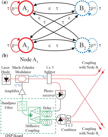
Figure 1: (Color online) (a) Schematic of four nodes separated into two groups, A (red, solid) and B (blue, dashed). (b) Experimental setup of a single node, showing coupling to the other nodes according to the configuration in (a).

The experimental setup consists of four optoelectronic feedback loops, which act as the four nodes of the network. We consider several coupling schemes. In the first one, the nodes are coupled together in the configuration shown in Fig. 1(a) in order to form two groups. There are no direct coupling links between two nodes in the same group. However, a node is coupled bidirectionally to both of the nodes in the other group. In this experiment, the coupling strength, $\varepsilon$, and coupling delay, $\tau$, are the same for all coupling links. However, the parameters of the nodes differ depending on which group the nodes are in. Both of the nodes in group A are identical, and both of the nodes in group B are identical, but the nodes in group A are not identical to the nodes in group B. In Fig. 1(a), the coupling links are shown in black (arrows in each direction to indicate bidirectional coupling), and the self-feedback of the nodes is indicated by the gray (colored) lines and arrows.

A schematic of a single node is shown in Fig. 1(b), where red lines indicate optical fibers, and black or green lines indicate electronic paths. In each node, light from a diode laser passes through a Mach-Zehnder modulator (MZM), whose output light intensity is $\cos^{2}(x+\phi_{0})$ for an input voltage signal $x$. There is a controllable bias phase of the MZM, which we set to be $\phi_{0}=\frac{\pi}{4}$. The optical signal is split into three equal signals: one is the feedback signal, and the other two are the coupling to the two nodes in the opposite group. A photoreceiver converts the feedback optical signal to an electrical signal, which is one of the two inputs to the DSP (digital signal processing) board. The incoming optical signals from the two nodes of the other group are combined optically before a second photoreceiver converts the composite coupled signal to an electronic signal, which is the second input of the DSP board. The DSP board implements the feedback and coupling time delays, which are the same for this experiment ($\tau=1.4$ ms), and a diffusive coupling scheme. The feedback signal is scaled by a factor of $1-\varepsilon$, while each incoming signal to a node is scaled by a factor of $\frac{\varepsilon}{n_{\text{in}}}$, for the global coupling strength, $\varepsilon$, and the number of links incoming to a node, $n_{\text{in}}$. For the configuration shown in Fig. 1(a), $n_{\text{in}}=2$ for all nodes, but in general, $n_{\text{in}}$ can be different for each node. The feedback and coupled signals are summed on the DSP board.

The DSP board also implements a digital filter, which is a two-pole bandpass filter with cutoff frequencies at 100 Hz and 2.5 kHz and a sampling rate of 24 kSamples/s, and also scales the combined signal by a scale factor, which controls the feedback strength, which we denote $\beta$. The output of the DSP board is amplified with a voltage amplifier, whose output drives the MZM. Although $\beta$ is a combination of gains of the photoreceiver, amplifier, and other components, the DSP board is the only place where the gain is changed.

For this experiment, all parameters except for $\beta$ are identical in all four nodes. We keep $\beta$ identical among the members of each group but allow a different $\beta$ for each group, denoted by $\beta^{(A)}$ and $\beta^{(B)}$. Previous studies have revealed the wide variety of behaviors that are possible for this type of system, depending on the value of $\beta$ Murphy et al. (2010). For this study, we have used a range of $\beta$ from 0 to 10, with the experiments focusing on cases of $\beta>3$, for which the system displays chaos (with some periodic windows) when the nodes are not coupled.

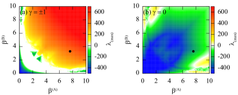
Figure 2: (Color online) Maximum Lyapunov exponent $\lambda_{\textnormal{max}}$ as a function of $\beta^{(A)}$ and $\beta^{(B)}$: (a) in the longitudinal directions $\gamma=\pm 1$, (b) in the transverse direction $\gamma=0$. White areas correspond to $\lambda_{\textnormal{max}}=0$. Black dot indicates values of $\beta^{(A)}$ and $\beta^{(B)}$ used in this experiment.

For each run of the experiment, the nodes are started from random initial conditions. This system has a time delay, so the initial condition will be a function of time. Thus, we record the random electrical activity at the input to the DSP in the absence of coupling and feedback for 1 second to provide the initial states for the nodes. After recording an initial condition, we enable feedback for 4 seconds, which is long enough for transients to disappear. At the end of this period, we enable coupling. Data are taken after transients have died out.

The system of coupled feedback loops can be well-described by a mathematical model with a system of time delay differential equations for the voltages input to the MZMs $x_{i}^{(m)}\in\mathbb{R}$ and the vectors describing the states of the filters $\mathbf{u}_{i}^{(m)}\in\mathbb{R}^{2}$ Murphy et al. (2010):

$$\mathbf{\dot{u}}_{i}^{(m)}(t)=\mathbf{E}\mathbf{u}_{i}^{(m)}(t)-\mathbf{F}\beta^{(m)}\cos^{2}(x_{i}^{(m)}(t-\tau)+\phi_{0}),$$ (1)

$$x_{i}^{(m)}(t)=\mathbf{G}[\mathbf{u}_{i}^{(m)}(t)+\varepsilon\sum_{j}K_{ij}^{(m)}(\mathbf{u}_{j}^{(m^{\prime})}(t)-\mathbf{u}_{i}^{(m)}(t))],$$ (2)

where $m$ and $m^{\prime}\not=m$ denote the groups A or B, and $i$ indicates the node within a group. $\mathbf{E}=(\begin{smallmatrix}-(\omega_{H}+\omega_{L})&-\omega_{L}\\ \omega_{H}&0\end{smallmatrix})$, $\mathbf{F}=(\begin{smallmatrix}\omega_{L}\\ 0\end{smallmatrix})$, and $\mathbf{G}=(\begin{smallmatrix}1&0\end{smallmatrix})$ are constant matrices that describe the filter. The filter parameters are chosen as $\omega_{L}=2\pi\cdot 2.5$ kHz and $\omega_{H}=2\pi\cdot 0.1$ kHz. For a bipartite network with no intra-group coupling, we define the inter-group coupling matrices $\mathbf{K}^{(m)}=\{K^{(m)}_{ij}\}$:

$$\mathbf{K}=\left(\begin{array}[]{cc}0&\mathbf{K}^{(A)}\\ \mathbf{K}^{(B)}&0\\ \end{array}\right),$$ (3)

where $\mathbf{K}$ is the overall coupling matrix for the entire network. For the configuration shown in Fig. 1(a), $i,j=1,2$, and $\mathbf{K}^{(A)}=\mathbf{K}^{(B)}=\frac{1}{2}(\begin{smallmatrix}1&1\\ 1&1\\ \end{smallmatrix})$ so that

$$\mathbf{K}=\left(\begin{array}[]{cc}0&\mathbf{K}^{(A)}\\ \mathbf{K}^{(B)}&0\\ \end{array}\right)=\frac{1}{2}\left(\begin{array}[]{cccc}0&0&1&1\\ 0&0&1&1\\ 1&1&0&0\\ 1&1&0&0\\ \end{array}\right).$$ (4)

Equations (1) and (2) can describe the dynamics of the uncoupled nodes if we set the coupling strength $\varepsilon=0$, as the second term in Eq. (2) represents the diffusive coupling scheme.

Numerical simulations use a discrete-time implementation of these differential equations, as described in Ref. Murphy et al. (2010). The simulations of uncoupled and coupled systems are in excellent agreement with the experimental results for the variety of dynamical behaviors that can be observed.

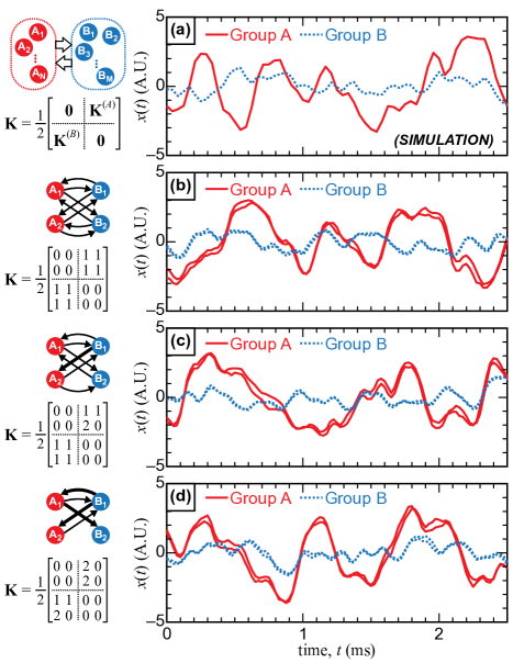
Figure 3: (Color online) (a) Simulated motion in the synchronization manifold, obtained by numerically solving Eqs. (6) and (7), showing the predicted group-synchronous state. (b),(c),(d) Experimentally measured time traces from three different network configurations (indicated by the coupling scheme and the coupling matrices $\mathbf{K}$) that achieve group synchrony. All three networks have the same eigenspectra, but the configuration in (b) is symmetric while those in (c) and (d) are not.

We will now investigate the existence and stability of the group synchronous solution, i.e., we will derive analytical conditions determining whether such a solution (in which the two nodes of each group are identically and isochronously synchronized, but there is no identical synchrony between nodes of different groups) exists for given values of $\beta^{(A)}$ and $\beta^{(B)}$, and if it does, if that solution is stable. We use the approach described in Sorrentino and Ott (2007); Dahms et al. (2012). The condition for the existence of the group synchronous solution for a particular coupling configuration is that

$$\sum_{j}K_{ij}^{(m)}=c^{(m)},m=\{A,B\},$$ (5)

i.e., that the row sum of the matrices $\mathbf{K}^{(m)}$ is constant. For the work reported here, we fix $c^{(A)}=c^{(B)}=1$.

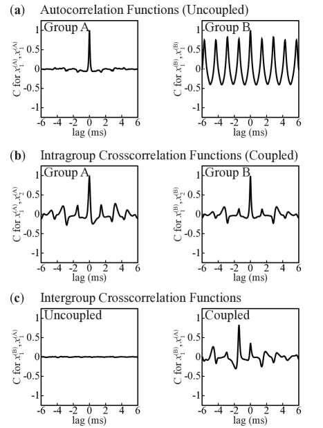
Figure 4: Correlation functions of 3.9 s of experimental data. (a) Autocorrelation functions for the dynamics of group A (left) and group B (right), with no coupling in the system. (b) Cross-correlation functions between the two nodes in group A (left) and group B (right), for coupled nodes. (c) Cross-correlation functions between one node in group A and one node in group B for the uncoupled system (left) and coupled system (right).

The group synchronized dynamics for group m is given by

$$\dot{\mathbf{u}}_{s}^{(m)}(t)=\mathbf{E}\mathbf{u}_{s}^{(m)}(t)\\ -\mathbf{F}\beta^{(m)}\cos^{2}(x_{s}^{(m)}(t-\tau)+\phi_{0}),$$ (6)

$$x_{s}^{(m)}(t)=\mathbf{G}[(\mathbf{u}_{s}^{(m)}(t)+\varepsilon(\mathbf{u}_{s}^{(m^{\prime})}(t)-\mathbf{u}_{s}^{(m)}(t))].$$ (7)

Linearizing Eqs. (1) and (2) about the synchronous solution $\mathbf{u}_{s}^{(m)}$ ($m=A,B$), we obtain the master stability equations:

$$\begin{split}\delta\dot{\mathbf{u}}^{(m)}(t)=&\mathbf{E}\delta\mathbf{u}^{(m)}(t)-\mathbf{F}\beta^{(m)}\sin(2x_{s}^{(m)}(t-\tau)+2\phi_{0})\\ &\times\mathbf{G}[(1-\varepsilon)\delta\mathbf{u}^{(m)}(t-\tau)+\varepsilon\gamma\mathbf{u}^{(m^{\prime})}(t-\tau)].\end{split}$$ (8)

In Eq. (8), $\gamma$ is a parameter that is chosen from the eigenvalue spectrum of $\mathbf{K}$. The largest Lyapunov exponent as a function of this parameter $\gamma$ is called the MSF. For the configurations presented here, the nonzero eigenvalues of $\mathbf{K}$ are 1 and -1, and any remaining eigenvalues are zeros. Therefore, the stability results will be identical for any two-group network whose nodes are described by Eqs. (1) and (2) and whose coupling matrix is in the form of (3), satisfies (5), and has identical rows for either $\mathbf{K}^{(A)}$ or $\mathbf{K}^{(A)}$ (for a proof, see supplemental material).

The eigenvalues $\gamma=-1$ and $\gamma=1$ in the master stability equation (8) correspond to perturbations parallel to the synchronization manifold. The corresponding value of the MSF determines the dynamical behavior inside the synchronization manifold and is shown in Fig. 2(a) in dependence on the parameters $\beta^{(A)}$ and $\beta^{(B)}$. Negative, zero, and positive values denote fixed-point, periodic, and chaotic dynamics, respectively. Due to the inversion symmetry of the MSF for two-group synchronization  Sorrentino and Ott (2007); Dahms et al. (2012), the MSF values are identical for $\gamma=-1$ and $\gamma=1$.

Transverse stability of the synchronization manifold is determined by using the eigenvalue $\gamma=0$ in Eq. (8). Figure 2(b) shows the largest Lyapunov exponent in the transverse direction, which is negative for almost the entire range of $\beta^{(A)}$ and $\beta^{(B)}$ that is shown, indicating that we expect the group synchronous solution to be stable for most parameters.

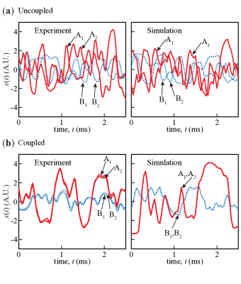
Figure S1: Comparison of time traces from experiment (left column) and simulation (right column). Nodes in group A (B) are indicated by the red and solid (blue and dashed) lines. (a) Nodes are uncoupled, and the uncoupled nodes are completely unsynchronized. (b) Nodes are coupled according to the configuration in Fig. 1(a). There is identical, isochronal synchrony between $x_{1}^{(A)}$ and $x_{2}^{(A)}$, and between $x_{1}^{(B)}$ and $x_{2}^{(B)}$, but not identical synchrony between the groups, so this is an example of group synchrony. In the simulation, the two traces in one group are exactly synchronized and are indistinguishable, as we expect from a simulation without noise or mismatch. In experiment, slight differences between synchronized traces arise from experimental noise and mismatch in the real experimental system. In both the experiment and simulation, the dynamics of the nodes in group B have a significantly smaller amplitude than those in group A, with qualitatively similar dynamics between simulation and experiment.

To observe group synchrony in this system, we select dissimilar values of $\beta^{(A)}$ and $\beta^{(B)}$, as shown by the black dots in Fig. 2. The global coupling strength is chosen as $\varepsilon=0.8$. The experimental values for $\beta^{(A)}$ and $\beta^{(B)}$ were adjusted using the DSP board. The values of $\beta^{(A)}$ and $\beta^{(B)}$ used in simulation were established by varying the values close to the experimental values to find nearby values which match best the dynamical behavior of the experiments for uncoupled nodes, obtained from the shape of the reconstructed attractor in phase space. Since the values determined experimentally as $\beta^{(A)}=7.6$ and $\beta^{(B)}=3.3$ are subject to measurement uncertainties, it is not surprising that we find slightly different values in simulation, i.e., $\beta^{(A)}=7.66$ and $\beta^{(B)}=3.28$. Comparison of uncoupled and coupled time traces in experiment and simulation is shown in the supplemental material, Fig. S1.

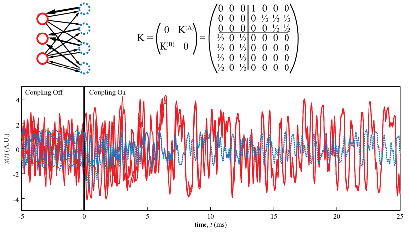
Figure S2: Simulation of a seven node network displaying group synchrony. The coupling scheme and the associated coupling matrix are shown above the simulated time traces. The parameters are the same as those presented in the letter. Coupling is enabled at time $t=0$, and the nodes become group synchronized so that all three red, solid lines of Group A are identically synchronized, and all four blue, dashed traces of Group B are identically synchronized. Note that the coupling matrix for the specific network configuration shown here satisfies Eq. (S7j). Hence, the coupling matrix has eigenvalues -1, 1, and degenerate zeros. The stability of the group synchronous solution of this system is described by Fig. 2(b). The dynamics of the seven node, group synchronized system, are predicted by Fig. 2(a), as illustrated by Fig. 3(a).

Figure 3 shows experimental and simulated time traces of the coupled system. The simulated traces in Fig. 3(a) show the behavior of any two-group system displaying stable group synchrony according to Eqs. (6) and (7), with the parameters we have used here. Figure 3(b) shows experimental results for a system coupled according to Fig. 1(a). These time traces show that there is identical, isochronal synchrony between $x_{1}^{(A)}$ and $x_{2}^{(A)}$, and between $x_{1}^{(B)}$ and $x_{2}^{(B)}$, but not identical synchrony between the groups. Thus, this is an example of group synchrony. We also performed experiments on two asymmetric four-node configurations. These configurations were created by removing links from the original structure of Fig. 1(a), while preserving the constant row sum and eigenvalues (1, -1, 0, and 0) of $\mathbf{K}$, keeping all other parameters the same. Their topologies and dynamics are shown in Figs. 3(c) and 3(d). Because these schemes are also described by Fig. 2, they also display group synchrony. In the experimental time traces, there are slight differences between the two traces of one group, due to the intrinsic experimental noise and mismatch we expect in any real system. An example of a larger network that displays the same behavior is presented in the supplemental material, Fig. S2.

To further examine the nature of the synchrony of this system, we calculate the correlation functions of the experimental time traces, as shown in Fig. 4 for the topology shown in Fig. 1(a). For two variables $y(t)$ and $z(t)$, which each have a mean of zero, we define the correlation function $C$ as a function of time lag $\Delta t$ Mulet et al. (2004):

$$C(\Delta t)=\frac{\langle y(t)z(t+\Delta t)\rangle}{\sqrt{\langle y^{2}(t)\rangle\langle z^{2}(t)\rangle}}.$$ (9)

Figure 4(a) shows the autocorrelation functions for one node in each group when the nodes are uncoupled. The autocorrelation of $x_{1}^{(A)}$ shows only a peak at zero time lag, which indicates chaotic dynamics, while the autocorrelation of $x_{1}^{(B)}$ shows periodic dynamics, with correlation peaks at intervals of the time delay $\tau=1.4$ ms. In Fig. 4(b), we show the cross-correlation functions of $x_{1}^{(A)}$ with $x_{2}^{(A)}$, and of $x_{1}^{(B)}$ with $x_{2}^{(B)}$ for the coupled system, which confirms identical, isochronal chaotic synchronization between the two nodes in a single group. Figure  4(c) shows the cross-correlation functions between two nodes in different groups, without and with coupling. The uncoupled case has no correlation, as we expect, but the coupled case has a high correlation peak at a lag of $\Delta t=-1.4$ ms. From this, we can see that there is time-lagged phase synchrony between the two groups, with the dynamics of group B leading the dynamics of group A by the system delay, $\tau$. However, the amplitudes of fluctuations of the two groups are still different after coupling, so there is no complete synchronization, and we have an interesting situation of the simultaneous coexistence of intragroup isochronal identical synchrony and time-lagged phase synchrony between the groups.

In conclusion, we have examined a four-node system of nonlinear optoelectronic oscillators in the case where there are two groups of nodes with dissimilar parameters. Our experiments display the phenomenon of group synchronization, and we analyze the stability of the group synchronized solutions for chaotic dynamical states. It is remarkable that, although the coupling is entirely between the different groups and not within the groups, identical isochronal synchronization within each group is induced by this coupling, while the two groups are not mutually amplitude synchronized, as predicted by our stability analysis using the generalized master stability function Sorrentino and Ott (2007); Dahms et al. (2012). Thus the nodes of group B act as a kind of dynamical relay Fischer et al. (2006) for the nodes of group A, and vice versa. These results have been experimentally demonstrated with three coupling configurations, and conditions for observing group synchrony in other networks have been discussed.

Our observations go beyond previous work on sublattice and cluster synchrony, where the experiments focused on optical phase synchronization for coupled lasers without self-feedback Aviad et al. (2012); Nixon et al. (2011). Group synchronization in larger networks is a significant challenge for future experimental investigation.

This work was supported by DOD MURI grant ONR N000140710734 and by DFG in the framework of SFB 910. The authors would like to acknowledge helpful comments from I. Kanter and L. Pecora.

I Supplemental Material

Figures 3(b), 3(c), and 3(d) show that stable group synchrony is experimentally observed for three different coupling configurations. Here we show that our stability analysis and the numerical computations in Fig. 2 apply to all of these coupling schemes and, more generally, to a whole class of networks, characterized by an arbitrary number of nodes in both the groups $A$ and $B$.

We define $N_{A}$ and $N_{B}$ the number of nodes in group $A$ and $B$, respectively. Then the couplings are fully described by the $N_{A}\times N_{B}$ coupling matrix $\mathbf{K}^{(A)}$, whose entries $\{K^{(A)}_{ij}\}$ represent the intensity of the direct interaction from system $j$ in group $B$ to $i$ in group $A$ and the $N_{B}\times N_{A}$ matrix $\mathbf{K}^{(B)}$, whose entries $\{K^{(B)}_{ij}\}$ represent the intensity of the direct interaction from system $i$ in group $A$ to $j$ in group $B$.

First we note that the motion in the synchronization manifold (Eqs. (6) and (7)) applies to any network described by Eqs. (1) and (2), as long as the entries along the rows of the matrices $\mathbf{K}^{(A)}$ and $\mathbf{K}^{(B)}$ sum to one. Thus in what follows, we will limit our attention to the case that

$$c^{(A)}=c^{(B)}=1.$$ (S1)

If assumption (S1) is verified, it follows that the maximum Lyapunov exponent of the synchronous solution shown in Fig. 2(a) does not depend on the details of the underlying network structure.

According to Ref. Sorrentino and Ott (2007), a master stability function approach to group synchronization is possible for any network described by Eqs. (1) and (2), under the assumption (S1). For any such network stability depends on the eigenvalues of the matrix

$$\mathbf{K}=\left(\begin{array}[]{cc}0&\mathbf{K}^{(A)}\\ \mathbf{K}^{(B)}&0\\ \end{array}\right).$$ (S2)

From Ref. Sorrentino and Ott (2007) we see that these eigenvalues are

$$\Lambda=[0,0,...,0]\bigcup[\pm\sqrt{\tilde{\lambda}_{1}},\pm\sqrt{\tilde{\lambda}_{2}},...,\pm\sqrt{\tilde{\lambda}_{{N}_{min}}}],$$ (S3)

where $[0,0,...,0]$ denotes $|N_{A}-N_{B}|$ zeros and $\tilde{\Lambda}=\{\tilde{\lambda}_{1},...,\tilde{\lambda}_{{N}_{min}}\}$ denotes the spectrum of the $N_{min}\times N_{min}$ matrix,

$$D=\left\{\begin{array}[]{ccc}{\mathbf{K}^{(A)}\mathbf{K}^{(B)},}\quad\mbox{if}\quad{N_{A}\leq N_{B},}\\ {\mathbf{K}^{(B)}\mathbf{K}^{(A)},}\quad\mbox{if}\quad{N_{B}<N_{A},}\end{array}\right.$$ (S6)

We proceed now under the assumption that either one of the two following conditions is satisfied,

$$\mathbf{K}^{(A)}=\left(\begin{array}[]{cccc}a\\ a\\ ...\\ a\end{array}\right),$$ (S7e)

$$\mathbf{K}^{(B)}=\left(\begin{array}[]{cccc}b\\ b\\ ...\\ b\end{array}\right),$$ (S7j)

where $a$ ($b$) is any $N_{B}$-dimensional row-vector ($N_{A}$-dimensional row-vector) with its entries summing to one. Then the matrix $D$ is in the form

$$D=\left(\begin{array}[]{cccc}d\\ d\\ ...\\ d\end{array}\right),$$ (S8)

where $d$ is an $N_{min}$-dimensional row-vector with sum of its entries equal one. Note that the underlying assumption is that either one of the matrices $\mathbf{K}^{(A)}$ and $\mathbf{K}^{(B)}$ is in the form of Eq. (S7) (not necessarily both). Then the eigenvalue equation for the matrix $D$ reduces to the following equation

$$\lambda v_{i}=d\cdot v=\ell\quad\quad i=1,...,N_{min},$$ (S9)

where $v=[v_{1},v_{2},...,v_{N_{min}}]$ is an eigenvector, $\lambda$ is the associated eigenvalue, and $\ell$ is a constant that does not depend on $i$. There are two possible solutions for Eq. (S9):

(i) $\ell=0$. Then, $\lambda=0$ and $v$ is any vector orthogonal to $d$. There are $(N_{min}-1)$ such vectors.

(ii) $\ell\neq 0$. Then, $v_{1}=v_{2}=...=v_{N_{min}}$ and from the sum of the entries of the vector $d$ being equal one, it follows that $\lambda=1$.

Hence by using Eq. (S3), and assuming satisfaction of either one of the Eqs. (S7e) or (S7j), the eigenvalues of the matrix $K$ are

$$\Lambda=[0,0,...,0]\bigcup[-1,1],$$ (S10)

where here $[0,0,...,0]$ denotes $|N_{A}+N_{B}-2|$ zeros. It follows that stability of the group synchronous solution for any network that satisfies either Eqs. (S7(a)) or (S7(b)) is described by the plot in Fig. 2(b).

References

- Albert and Barabási (2002) R. Albert and A.-L. Barabási, Rev. Mod. Phys. 74, 47 (2002).
- Boccaletti et al. (2006) S. Boccaletti, V. Latora, Y. Moreno, M. Chavez, and D.-U. Hwang, Phys. Reports 424, 175 (2006).
- Pecora and Carroll (1990) L. M. Pecora and T. L. Carroll, Phys. Rev. Lett. 64, 821 (1990).
- Pikovsky et al. (2001) A. S. Pikovsky, M. G. Rosenblum, and J. Kurths, Synchronization, A Universal Concept in Nonlinear Sciences (Cambridge University Press, Cambridge, 2001).
- Pecora and Carroll (1998) L. M. Pecora and T. L. Carroll, Phys. Rev. Lett. 80, 2109 (1998).
- Buldu et al. (2007) J. M. Buldu, M. C. Torrent, and J. Garcia-Ojalvo, J. Lightwave Techn. 25, 1549 (2007).
- González et al. (2007) C. M. González, C. Masoller, M. C. Torrent, and J. García-Ojalvo, Europhys. Lett. 79, 64003 (2007).
- Kestler et al. (2007) J. Kestler, W. Kinzel, and I. Kanter, Phys. Rev. E 76, 035202 (2007).
- Aviad et al. (2012) Y. Aviad, I. Reidler, M. Zigzag, M. Rosenbluh, and I. Kanter, Opt. Express 20, 4352 (2012).
- Nixon et al. (2011) M. Nixon, M. Friedman, E. Ronen, A. A. Friesem, N. Davidson, and I. Kanter, Phys. Rev. Lett. 106, 223901 (2011).
- Amann et al. (2008) A. Amann, A. Pokrovskiy, S. Osborne, and S. O’Brien, J. Phys. Conf. Series 138, 012001 (2008).
- Pigolotti et al. (2007) S. Pigolotti, S. Krishna, and M. H. Jensen, Proc. Natl. Acad. Sci. 104, 6533 (2007).
- Jensen et al. (2009) M. H. Jensen, S. Krishna, and S. Pigolotti, Phys. Rev. Lett. 103, 118101 (2009).
- Choe et al. (2010) C.-U. Choe, T. Dahms, P. Hövel, and E. Schöll, Phys. Rev. E 81, 025205 (2010).
- Kanter et al. (2011a) I. Kanter, E. Kopelowitz, R. Vardi, M. Zigzag, W. Kinzel, M. Abeles, and D. Cohen, Europhys. Lett. 93, 66001 (2011a).
- Kanter et al. (2011b) I. Kanter, M. Zigzag, A. Englert, F. Geissler, and W. Kinzel, Europhys. Lett. 93, 60003 (2011b).
- Kestler et al. (2008) J. Kestler, E. Kopelowitz, I. Kanter, and W. Kinzel, Phys. Rev. E 77, 046209 (2008).
- Sorrentino and Ott (2007) F. Sorrentino and E. Ott, Phys. Rev. E 76, 056114 (2007).
- Dahms et al. (2012) T. Dahms, J. Lehnert, and E. Schöll, Phys. Rev. E 86, 016202 (2012).
- Kouomou et al. (2005) Y. C. Kouomou, P. Colet, L. Larger, and N. Gastaud, Phys. Rev. Lett. 95, 203903 (2005).
- Peil et al. (2009) M. Peil, M. Jacquot, Y. K. Chembo, L. Larger, and T. Erneux, Phys. Rev. E 79, 026208 (2009).
- Murphy et al. (2010) T. E. Murphy, A. B. Cohen, B. Ravoori, K. R. B. Schmitt, A. V. Setty, F. Sorrentino, C. R. S. Williams, E. Ott, and R. Roy, Phil. Trans. R. Soc. A 368, 343 (2010).
- Callan et al. (2010) K. E. Callan, L. Illing, Z. Gao, D. J. Gauthier, and E. Schöll, Phys. Rev. Lett. 104, 113901 (2010).
- Rosin et al. (2011) D. P. Rosin, K. E. Callan, D. J. Gauthier, and E. Schöll, Europhys. Lett. 96, 34001 (2011).
- Ravoori et al. (2011) B. Ravoori, A. B. Cohen, J. Sun, A. E. Motter, T. E. Murphy, and R. Roy, Phys. Rev. Lett. 107, 034102 (2011).
- Mulet et al. (2004) J. Mulet, C. Mirasso, T. Heil, and I. Fischer, J. Opt. B 6, 97 (2004).
- Fischer et al. (2006) I. Fischer, R. Vicente, J. M. Buldú, M. Peil, C. R. Mirasso, M. C. Torrent, and J. García-Ojalvo, Phys. Rev. Lett. 97, 123902 (2006).