Highly polarized Fermi gases in two dimensions

Abstract

We investigate the highly polarized limit of a two-dimensional (2D) Fermi gas, where we effectively have a single spin-down impurity atom immersed in a spin-up Fermi sea. By constructing variational wave functions for the impurity, we map out the ground state phase diagram as a function of mass ratio $m_{\uparrow}/m_{\downarrow}$ and interaction strength. In particular, we determine when it is favorable for the dressed impurity (polaron) to bind particles from the Fermi sea to form a dimer, trimer or even larger clusters. Similarly to 3D, we find that the Fermi sea favors the trimer state so that it exists for $m_{\uparrow}/m_{\downarrow}$ less than the critical mass ratio for trimer formation in the vacuum. We also find a region where dimers have finite momentum in the ground state, a scenario which corresponds to the Fulde-Ferrell-Larkin-Ovchinnikov superfluid state in the limit of large spin imbalance. For equal masses ($m_{\uparrow}=m_{\downarrow}$), we compute rigorous bounds on the polaron-dimer transition, and we show that the polaron energy and residue is well captured by the variational approach, with the former quantity being in good agreement with experiment. When there is a finite density of impurities, we find that this polaron-dimer transition is preempted by a first-order superfluid-normal transition at zero temperature, but it remains an open question what happens at finite temperature.

I Introduction

The creation of tunable Fermi systems with ultracold atomic gases has greatly renewed interest in fermionic pairing phenomena and superfluidity. In particular, recent experiments have successfully confined fermionic atoms to a quasi-two-dimensional (quasi-2D) geometry Martiyanov et al. (2010); Fröhlich et al. (2011); Dyke et al. (2011); Feld et al. (2011); Sommer et al. (2012); Koschorreck et al. (2012); Zhang et al. (2012), thus enabling the investigation of 2D Fermi gases. Such model 2D systems can potentially provide insight into more complicated solid state systems such as electron-hole bilayers Croxall et al. (2008); Seamons et al. (2009) and high temperature superconductors Norman (2011). Moreover, 2D is the “marginal” dimension where quantum fluctuations are enhanced compared to 3D, leading to the destruction of Bose Einstein condensation (BEC) at finite temperature. At the same time, there is a dearth of exactly solvable models, in contrast to the case in 1D. This makes the cold-atom system even more important for testing theoretical approaches in 2D.

A canonical many-body problem currently under investigation is that of an impurity interacting with a medium. This so-called “polaron” problem traditionally involves a bosonic medium such as a bath of phonon excitations in a crystal Fröhlich (1954). However, the advent of cold atoms has extended this problem to include a fermionic medium, where the impurity can now undergo a sharp transition and effectively change its statistics by binding fermions from the background Fermi gas Prokof’ev and Svistunov (2008a, b). For a fermionic impurity, this corresponds to the highly polarized limit of a two-component ($\uparrow$, $\downarrow$) Fermi gas and, thus, the existence of such binding transitions will determine the topology of the phase diagram for the spin-imbalanced Fermi gas Parish et al. (2007a); Sheehy and Radzihovsky (2007). In 3D, the $\downarrow$ impurity is initially dressed by density fluctuations of the $\uparrow$ Fermi gas, forming a polaron state Chevy (2006), but with increasing attractive interactions it can bind an extra $\uparrow$ particle to form a dimer (molecule) Prokof’ev and Svistunov (2008a, b); Combescot et al. (2009); Mora and Chevy (2009); Punk et al. (2009); Mathy et al. (2011) or it can even bind two $\uparrow$ particles to form a trimer Mathy et al. (2011), depending on the mass ratio $m_{\uparrow}/m_{\downarrow}$. For the 2D case, there has been debate about whether strong quantum fluctuctions preclude the existence of such binding transitions Zöllner et al. (2011); Klawunn and Recati (2011), but one of us has recently argued that sharp polaron-molecule transitions can exist Parish (2011) and this appears consistent with experiment Koschorreck et al. (2012); Levinsen and Baur (2012).

In this work, we further investigate this issue by mapping out the ground state phase diagram for the 2D impurity problem as a function of mass ratio $m_{\uparrow}/m_{\downarrow}$ and interaction strength. Similarly to 3D, we show that the impurity can bind one, two or more $\uparrow$ particles from the Fermi sea to form bound clusters dressed by density fluctuations. We approximate the different impurity states using variational wave functions that include a finite number of particle-hole excitations of the Fermi sea. We find that the presence of a Fermi sea appears conducive to the formation of trimers, which in vacuum exist for $m_{\uparrow}/m_{\downarrow}>3.33$ Pricoupenko and Pedri (2010). On the other hand, tetramers containing three $\uparrow$ particles and existing for $m_{\uparrow}/m_{\downarrow}>5.0$ in vacuum Levinsen and Parish (2012), appear to be disfavored in the many-body system. We further find a region of parameter space in which the impurity binds a single particle from the Fermi sea to form a dimer with finite momentum. A finite density of such molecules will form a spatially modulated condensate and thus this state is the single-particle analog of the elusive Fulde-Ferrell-Larkin-Ovchinnikov (FFLO) phase Fulde and Ferrell (1964); Larkin and Ovchinnikov (1967).

The presence of bound clusters of $N+1$ particles such as trimers and tetramers ($N=2$ and 3) introduce important $(N+1)$-body correlations. Even if these states are metastable, their presence can still affect the system: for instance, we expect three-body correlations to be more important in 2D than in 3D for the mass-balanced system due to the smaller repulsive barrier between the identical fermions, and the resulting enhanced three-body interactions Levinsen et al. (2009); Ngampruetikorn et al. (2012). In order to quantify the effect of these higher order correlations, we consider the polaron state dressed by two particle-hole pairs for equal masses ($m_{\uparrow}=m_{\downarrow}$). This wavefunction includes three-body correlations, whereas the usual Chevy wavefunction Chevy (2006) contains only two-body correlations. The results of these two variational wavefunctions match in the limit of weak interactions and we also find a reasonable agreement across the regime of strong interactions. This approach further allows us to arrive at rigorous upper and lower bounds for the position of the polaron-molecule transition, yielding $-0.97<\ln(k_{F\uparrow}a_{2\rm{D}})<-0.802$, with $k_{F\uparrow}$ the Fermi momentum of majority $\uparrow$ particles and $a_{2\rm{D}}$ the 2D scattering length.

At any given interaction strength, only one state may be the ground state and all other states are at best metastable. The polaron wavefunction of Ref. Chevy (2006) leads to a completely real equation for the polaron’s energy, and thus one might think that the variational approach may only be used to calculate ground state properties of the polarized Fermi gas. On the other hand, using a diagrammatic approach as in Ref. Combescot et al. (2007) to describe the polaron, naturally incorporates an imaginary part in the energy, and thus the metastability of excited states is automatically present. We resolve this seeming discrepancy by showing here that a straightforward change of the variational wavefunction and the minimization procedure allows the variational approach to be extended to describe not only the ground state but also excited branches. Thus the two approaches are, in fact, fully equivalent.

The experimental observation of the transition from a polaron to a molecule may be precluded by phase separation into an unpolarized superfluid phase and a fully polarized normal phase. Using results from a quantum Monte Carlo (QMC) simulation of the superfluid phase in an equal-mass unpolarized Fermi gas Bertaina and Giorgini (2011), we indeed find this to be the case in the highly-polarized limit. However, this result only strictly applies to zero temperature and it remains an open question whether this occurs at finite temperature.

The paper is organized as follows: The contact interaction is introduced for the 2D system in Sec. II. Sections III and IV introduce the variational wave functions used to describe the possible ground states of the impurity atom, while Sec. V describes the resulting single-impurity phase diagrams. In Sec. VII we derive the condition for phase separation precluding the polaron-molecule transition, while in Sec. VI we introduce the polaron dressed by two particle-hole pairs. In Sec. VIII we show the manner in which the variational method may be modified to describe metastable states, and finally in Sec. IX we conclude.

II Preliminaries

We consider the Hamiltonian for a two-component atomic Fermi gas interacting via a short-range interaction in two dimensions (2D):

$$H= \sum_{{\mathbf{k}}\sigma}\epsilon_{{\mathbf{k}}\sigma}c^{\dagger}_{{\mathbf{k}}\sigma}c_{{\mathbf{k}}\sigma}+g\sum_{{\mathbf{k}},{\mathbf{k}^{\prime}},{\mathbf{q}}}c^{\dagger}_{{\mathbf{k}}\uparrow}c^{\dagger}_{{\mathbf{k}^{\prime}}\downarrow}c_{{\mathbf{k}^{\prime}}+{\mathbf{q}}\downarrow}c_{{\mathbf{k}}-{\mathbf{q}}\uparrow}~{},$$ (1)

where the spin $\sigma=\uparrow,\downarrow$, $\epsilon_{{\mathbf{k}}\sigma}=\frac{{\mathbf{k}}^{2}}{2m_{\sigma}}$, and $g$ is the strength of an attractive contact interaction. We work in units where $\hbar$ and the system area are both 1. Note that since we are considering low-energy, $s$-wave interactions, the Pauli exclusion suppresses interactions between the same species of fermion. For the two-body problem ($\uparrow$ and $\downarrow$), we simply have

$$-\frac{1}{g} =\sum_{{\mathbf{k}}}^{\Lambda}\frac{1}{\varepsilon_{B}+\epsilon_{{\mathbf{k}}\uparrow}+\epsilon_{{\mathbf{k}}\downarrow}},$$ (2)

where $\Lambda$ is the UV cut-off and $\varepsilon_{B}$ is the binding energy of the weakly bound diatomic molecule which always exists for an attractive interaction in 2D. We see that the integral logarithmically diverges if we fix $\varepsilon_{B}$ and take $\Lambda\to\infty$. Thus $\Lambda$ cannot be removed from the problem and the binding energy $\varepsilon_{B}$ depends on both $\Lambda$ and $g$, in contrast to 1D. For the many-body system, our results become independent of the cut-off $\Lambda$ once Eq. (2) is used to replace $g$ with $\varepsilon_{B}$.

At low energies, the elastic scattering of a spin-$\uparrow$ and a spin-$\downarrow$ atom at relative momentum $q$ is described by the $s$-wave scattering amplitude Landau and Lifshitz (1981)

$$f(q)=\frac{2\pi}{\ln\left[1/(qa_{2\rm{D}})\right]+i\pi/2}.$$ (3)

Here, the momentum dependence of the scattering amplitude is characterized by the 2D scattering length $a_{2\rm{D}}>0$. Analytic continuation of the scattering amplitude to momenta on the positive imaginary axis yields a pole in the scattering amplitude at $q=ia_{2\rm{D}}^{-1}$. This corresponds to the binding energy $\varepsilon_{B}=1/2m_{r}a_{2\rm{D}}^{2}$, with the reduced mass defined as $m_{r}=m_{\uparrow}m_{\downarrow}/(m_{\uparrow}+m_{\downarrow})$. Thus, the 2D scattering length essentially corresponds to the size of the two-body bound state. Unlike in 3D, the scattering amplitude in 2D does not reduce to a constant at low scattering momenta; instead the scattering is strong in the regime $\ln(qa_{2\rm{D}})\sim 0$ and weak when $|\ln(qa_{2\rm{D}})|\gg 1$. In the presence of a Fermi sea, the characteristic momentum scale is set by the Fermi momentum $k_{F}$ and we thus expect strong many-body effects when $\ln(k_{F}a_{2\rm{D}})\sim 0$. Indeed, Bloom Bloom (1975) has demonstrated how the 2D Fermi gas in the regime $|\ln(k_{F}a_{2\rm{D}})|\gg 1$ is perturbative in $1/\ln(k_{F}a_{2\rm{D}})$.

In the following, we focus on the case where we have a single spin-down minority atom immersed in a non-interacting Fermi sea of spin-up atoms — the extreme limit of population imbalance. Note that the phase diagram we obtain for the single impurity atom is independent of impurity statistics and is thus also relevant to 2D Bose-Fermi mixtures. However, the focus of this paper will be on fermionic impurities. Defining the interaction parameter in the imbalanced gas, $\eta\equiv\ln(k_{F\uparrow}a_{2\rm{D}})$, in the limit of weak attractive interactions (or, equivalently, the large-density limit) where $\eta\gg 1$, the ground state is expected to approach that of the non-interacting system: $\left|{P_{1}({\bf 0})}\right.\rangle=c^{\dagger}_{{\bf 0}\downarrow}\left|{FS}\right.\rangle$, where $\left|{FS}\right.\rangle$ represents the Fermi sea of $\uparrow$-particles. Note that the subscript on the “polaron” wave function $\left|{P}\right.\rangle$ denotes the number of operators acting on the Fermi sea; this is the nomenclature we will use throughout the paper. Decreasing $\eta$ will eventually give rise to one or more binding transitions, where the spin-down minority particle binds one or more spin-up particles. The behaviour of the system in this regime can be analysed with the use of variational wave functions for the different bound states.

III “Undressed” wave functions

In this section, we neglect the particle-hole excitations generated by the impurity $\downarrow$-particle interacting with the Fermi sea and focus on the “bare” part of the exact wave function. For the molecule and polaron, this is equivalent to the mean field approach for the spin-imbalanced Fermi gas (see, e.g., Ref. Parish et al. (2007b)). In the present problem of a single impurity interacting with a Fermi gas, the approach serves as a useful introduction to the more complicated wavefunctions dressed by particle-hole fluctuations. It should also provide insight into the relevant few-body correlations present in the system. Below, in Sec. IV, we consider wave functions dressed by one particle-hole excitation, an approach which yields quantitatively accurate results in the perturbative regimes of weak and strong attractive interactions and which is also expected to give a good description across the regime of strong 2D interactions $\eta\sim 0$, as we discuss below.

The results of this section become exact in the vacuum limit, $k_{F\uparrow}\to 0$. In this case, we can study transitions between different few-body states containing a single spin-$\downarrow$ atom and $N$ spin-$\uparrow$ particles. In vacuum, a bound diatomic molecule always exists for two atoms interacting via contact interactions under a strong two-dimensional confinement. Additionally, a trimer state consisting of two heavy fermions and one light particle becomes energetically favorable for a mass ratio $r\equiv m_{\uparrow}/m_{\downarrow}$ above 3.33 Pricoupenko and Pedri (2010), while a tetramer containing three heavy fermions and one light particle is favorable for $r>5.0$ Levinsen and Parish (2012).

III.1 Molecules ($M_{2}$)

The simplest, lowest-order variational wave function for a bound pair or “molecule” is:

$$\left|{M_{2}({\mathbf{p}})}\right.\rangle =\sum_{{\mathbf{k}}}\varphi_{{\mathbf{k}}}^{({\mathbf{p}})}c^{\dagger}_{{\mathbf{p}}-{\mathbf{k}}\downarrow}c^{\dagger}_{{\mathbf{k}}\uparrow}\left|{FS}\right.\rangle,$$ (4)

where ${\mathbf{p}}$ corresponds to the center-of mass momentum of the pair, while the spin-up particle momentum satisfies $k\equiv|{\mathbf{k}}|>k_{F\uparrow}$. This wave function gives the exact two-body state in the limit $k_{F\uparrow}\to 0$ and is in fact identical to the BCS mean field wave function for extreme imbalance (after the state with one $\downarrow$ particle has been projected out). Note that we assume the wave function (4) has one less $\uparrow$ particle in the Fermi sea compared with the non-interacting state $\left|{P_{1}}\right.\rangle$ in order to preserve particle number. Indeed, we will assume throughout this paper that all the impurity wave functions we introduce have the same number of $\uparrow$ particles as $\left|{P_{1}}\right.\rangle$. This is equivalent to measuring the energy of $\uparrow$ particles with respect to their chemical potential, the Fermi energy $E_{F\uparrow}\equiv k_{F\uparrow}^{2}/2m_{\uparrow}$, and thus we define $\xi_{{\bf k}\uparrow}\equiv\epsilon_{{\bf k}\uparrow}-E_{F\uparrow}$.

Minimizing the expectation value $\langle\left.{M_{2}({\mathbf{p}})}\right|(H-E)\left|{M_{2}({\mathbf{p}})}\right.\rangle$ with respect to $\varphi_{{\mathbf{k}}}^{({\mathbf{p}})}$ yields an implicit equation for the molecule energy $E$:

$$-\frac{1}{g} =\sum_{{\mathbf{k}}}\frac{1}{-E+\xi_{{\bf k}\uparrow}+\epsilon_{{\mathbf{p}}-{\mathbf{k}}\downarrow}}.$$ (5)

Here and in what follows we use the convention that the momentum ${\bf k}$ corresponds to a particle excited out of the Fermi sea, i.e. $|{\bf k}|>k_{F\uparrow}$. Additionally, the energy $E$ is assumed to be with respect to the (macroscopic) energy of the non-interacting $\uparrow$ Fermi gas. We neglect Hartree terms involving $gk_{F\uparrow}^{2}/4\pi$ since these vanish when we take the limit $\Lambda\to\infty$, $g\to 0$. Converting sums into integrals and sending $\Lambda\to\infty$ then gives:

$$2\varepsilon_{B} =-E^{\prime}-\frac{p^{2}(r-1)r}{2m_{r}(1+r)^{2}}+\frac{1}{1+r}\sqrt{\left(E^{\prime}+\left(E^{\prime}+\frac{k_{F\uparrow}^{2}}{2m_{r}}-\frac{(p-k_{F\uparrow})^{2}}{2m_{r}}\right)r\right)\left(E^{\prime}+\left(E^{\prime}+\frac{k_{F\uparrow}^{2}}{2m_{r}}-\frac{(p+k_{F\uparrow})^{2}}{2m_{r}}\right)r\right)}.$$

where we defined the energy $E^{\prime}=E-\frac{k_{F\uparrow}^{2}}{2m_{\downarrow}}$. Clearly, when we approach the two-body limit ($k_{F\uparrow}\to 0$), the molecule has its lowest energy at zero momentum. For this case, we simply have $E=\frac{k_{F\uparrow}^{2}}{2m_{\downarrow}}-\varepsilon_{B}$. However, once $k_{F\uparrow}a_{2\rm{D}}>1/\sqrt{r}$, we find that the molecule acquires a finite momentum:

$$p =\frac{1+r}{ra_{2\rm{D}}}\sqrt{k_{F\uparrow}a_{2\rm{D}}\sqrt{r}-1}.$$ (6)

Increasing $k_{F\uparrow}a_{2\rm{D}}$ further eventually causes the molecule to unbind into the state $\left|{P_{1}({\bf 0})}\right.\rangle$. At this unbinding transition (assuming there is a direct transition), we always find that $p=k_{F\uparrow}$, in contrast to the 3D case where $p=0$ for mass ratios sufficiently close to one Mathy et al. (2011). Referring to Eq. (6), this means that the molecule unbinds when $k_{F\uparrow}a_{2\rm{D}}=(1+r)/\sqrt{r}$, i.e. when $\varepsilon_{B}$ equals the center-of-mass kinetic energy of the molecule at $p=k_{F\uparrow}$.

III.2 Trimers ($T_{3}$)

Another possible bound state is the trimer consisting of two spin-up fermions and one spin-down particle. Since this trimer involves identical fermions, its angular momentum $L$ must necessarily be odd and so the lowest-energy trimer is a $p$-wave ($L=1$) bound state. Indeed, it may be regarded as a $p$-wave pairing of spin-up fermions mediated by their $s$-wave interactions with the spin-down particle. The lowest-order variational wave function for the trimer is

$$\left|{T_{3}({\bf 0})}\right.\rangle =\sum_{{\mathbf{k}_{1}}{\mathbf{k}_{2}}}\gamma_{{\mathbf{k}_{1}}{\mathbf{k}_{2}}}c^{\dagger}_{-{\mathbf{k}_{1}}-{\mathbf{k}_{2}}\downarrow}c^{\dagger}_{{\mathbf{k}_{1}}\uparrow}c^{\dagger}_{{\mathbf{k}_{2}}\uparrow}\left|{FS}\right.\rangle.$$ (7)

Since angular and linear momentum do not commute, we restrict ourselves to trimers with zero center-of-mass momentum (${\mathbf{p}}={\bf 0}$) in order to have a well-defined $L$. Such a restriction is unlikely to be drastic since there is no physical reason to believe that the trimer will have its lowest energy at finite momentum. In fact, we would generally expect the energy to be higher at non-zero ${\mathbf{p}}$ since the wave function would then contain an admixture of higher-energy angular momentum states $L>1$.

Minimizing $\langle\left.{T_{3}}\right|(H-E)\left|{T_{3}}\right.\rangle$ and defining the function $f_{{\mathbf{k}}_{2}}=\sum_{{\mathbf{k}}_{1}}\gamma_{{\bf k}_{1}{\bf k}_{2}}$ then results in the equation

$$f_{{\bf k}_{2}}\left[\frac{1}{g}+\sum_{{\mathbf{k}_{1}}}\frac{1}{E_{{\mathbf{k}_{1}}{\mathbf{k}_{2}}}}\right] =\sum_{{\mathbf{k}_{1}}}\frac{f_{{\mathbf{k}_{1}}}}{E_{{\mathbf{k}_{1}}{\mathbf{k}_{2}}}},$$ (8)

where $E_{{\mathbf{k}_{1}}{\mathbf{k}_{2}}}=-E+\epsilon_{{\mathbf{k}_{1}}+{\mathbf{k}_{2}}\downarrow}+\xi_{{\bf k}_{1}\uparrow}+\xi_{{\bf k}_{2}\uparrow}$. For $L=1$, we have $f_{\mathbf{k}}=\tilde{f}_{k}e^{i\phi}$, where $\phi$ is the angle with respect to the $x$-axis and $\tilde{f}$ is an arbitrary function. Performing the angular integration, leaves a one-dimensional integral equation for $\tilde{f}_{k}$ which is subsequently solved by discretizing $k$-space and converting the integral equation into a matrix eigenvalue equation Delves and Mohamed (1985). We emphasize that at this order of approximation, the effect of the Fermi sea is only taken into account in Eq. (8) through the restriction on the momenta in the sums ($|{\bf k}_{1}|>k_{F\uparrow}$). The energy of the trimer in the absence of a Fermi sea is recovered upon taking the limit $k_{F\uparrow}\to 0$.

III.3 The N+1 problem

The above approach may obviously be extended to the bound state consisting of a single spin-$\downarrow$ impurity and $N$ spin-$\uparrow$ particles:

$$\left|{X_{N+1}}\right.\rangle=\sum_{{\bf k}_{1}\ldots{\bf k}_{N}}\chi_{{\bf k}_{1}\ldots{\bf k}_{N}}c^{\dagger}_{-{\bf k}_{1}\ldots-{\bf k}_{N}\downarrow}c^{\dagger}_{{\bf k}_{1}\uparrow}\ldots c^{\dagger}_{{\bf k}_{N}\uparrow}\left|{FS}\right.\rangle.$$ (9)

Again, minimizing $\langle\left.{X_{N+1}}\right|(H-E)\left|{X_{N+1}}\right.\rangle$ and defining $f_{{\bf k}_{2}\ldots{\bf k}_{N}}=\sum_{{\bf k}_{1}}\chi_{{\bf k}_{1}\ldots{\bf k}_{N}}$ yields an equation for the energy of the $N+1$ bound state:

$$f_{{\bf k}_{2}\ldots{\bf k}_{N}}\left[\frac{1}{g}+\sum_{{\bf k}_{1}}\frac{1}{E_{{\bf k}_{1}\ldots{\bf k}_{N}}}\right]=$$

$$\sum_{{\bf k}_{1}}\frac{f_{{\bf k}_{1}{\bf k}_{3}\ldots{\bf k}_{N}}+f_{{\bf k}_{2}{\bf k}_{1}{\bf k}_{4}\ldots{\bf k}_{N}}+\ldots+f_{{\bf k}_{2}\ldots{\bf k}_{N-1}{\bf k}_{1}}}{E_{{\bf k}_{1}\ldots{\bf k}_{N}}},$$ (10)

where $E_{{\bf k}_{1}\ldots{\bf k}_{N}}=-E+\epsilon_{{\bf k}_{1}+\ldots+{\bf k}_{N}\downarrow}+\sum_{i}\xi_{{\bf k}_{i}\uparrow}$. This equation is explained in detail in Appendix A where an alternative derivation in terms of diagrams is presented.

Again the vacuum limit is recovered by letting $k_{F\uparrow}\to 0$ and we stress that Eq. (10) is quite general in this limit: It is equally valid for 1D, 2D and 3D systems; it may be extended to narrow Feshbach resonances by letting the coupling constant be energy dependent; and it may be used to treat the quasi-2D problem as in Ref. Levinsen and Parish (2012), if one includes a summation over harmonic oscillator modes. The equation satisfied by the tetramer energy ($N=3$) in this limit was obtained for the 3D problem in Ref. Castin et al. (2010), the equation for the $N+1$ problem in a quasi-2D geometry was derived in Ref. Levinsen and Parish (2012). Finally, Ref. Minlos (1995) derived an expression similar to our Eq. (10) for the 3D $N+1$ vacuum problem not (a) and Ref. Pricoupenko (2011) generalized this result to include also 1D and 2D.

IV Wave functions with one particle-hole excitation

We can improve on the wave functions in Sec. III by adding a single particle-hole excitation on top of the Fermi sea. We expect these improved wave functions (which are perturbative in the number of particle-hole excitations) to provide a reasonably accurate estimate of the single-impurity energy even in the regime of strong interactions, $k_{F\uparrow}a_{2\rm{D}}\sim 1$, since it has been argued that contributions from two or more particle-hole excitations nearly cancel out via destructive interference Combescot and Giraud (2008). We further investigate the validity of this approach in Sec. VI where we present our results for the impurity dressed by two particle hole pairs.

IV.1 Polarons ($P_{3}$)

Adding one particle-hole excitation to the non-interacting state $\left|{P_{1}}\right.\rangle$ gives the improved polaron wave function:

$$\left|{P_{3}({\mathbf{p}})}\right.\rangle =\alpha_{0}^{({\mathbf{p}})}c^{\dagger}_{{\mathbf{p}}\downarrow}\left|{FS}\right.\rangle+\sum_{{\mathbf{k}}{\mathbf{q}}}\alpha_{{\mathbf{k}}{\mathbf{q}}}^{({\mathbf{p}})}c^{\dagger}_{{\mathbf{p}}+{\mathbf{q}}-{\mathbf{k}}\downarrow}c^{\dagger}_{{\mathbf{k}}\uparrow}c_{{\mathbf{q}}\uparrow}\left|{FS}\right.\rangle,$$ (11)

where we have now included a center-of-mass momentum ${\mathbf{p}}$. Minimizing $\langle\left.{P_{3}({\mathbf{p}})}\right|(H-E)\left|{P_{3}({\mathbf{p}})}\right.\rangle$ then gives us equations:

$$\left(E-\epsilon_{{\mathbf{p}}\downarrow}\right)\alpha_{0}^{({\mathbf{p}})}=g\sum_{{\mathbf{k}}{\mathbf{q}}}\alpha_{{\mathbf{k}}{\mathbf{q}}}^{({\mathbf{p}})},$$ (12)

$$\left(E-\epsilon_{{\mathbf{p}}+{\mathbf{q}}-{\mathbf{k}}\downarrow}-\epsilon_{{\mathbf{k}}\uparrow}+\epsilon_{{\mathbf{q}}\uparrow}\right)\alpha_{{\mathbf{k}}{\mathbf{q}}}^{({\mathbf{p}})}=$$

$$g\sum_{{\mathbf{k}^{\prime}}}\alpha_{{\mathbf{k}^{\prime}}{\mathbf{q}}}^{({\mathbf{p}})}-g\sum_{{\mathbf{q}^{\prime}}} \alpha_{{\mathbf{k}}{\mathbf{q}^{\prime}}}^{({\mathbf{p}})}+g\alpha_{0}^{({\mathbf{p}})}.$$ (13)

We remind the reader that particle momenta ${\bf k}$ satisfy $|{\bf k}|>k_{F\uparrow}$. The hole momenta will be denoted by ${\bf q}$ with $|{\bf q}|<k_{F\uparrow}$. Combining Eqs. (12) and (13) gives an implicit equation for the energy,

$$E-\epsilon_{{\bf p}\downarrow}=\sum_{\bf q}\left[\frac{1}{g}+\sum_{\bf k}\frac{1}{E_{{\bf p}{\bf q}{\bf k}}-i0}\right]^{-1},$$ (14)

with $E_{{\bf p}{\bf q}{\bf k}}=-E+\xi_{{\bf k}\uparrow}-\xi_{{\bf q}\uparrow}+\epsilon_{{\bf p}+{\bf q}-{\bf k}\downarrow}$. Eq. (14) has two solutions: The attractive and repulsive polaron which have energies above and below the energy of the free impurity, respectively. Note that we must include here by hand a small imaginary part on the right hand side in order to describe the metastable repulsive polaron. We show in Sec. VIII how to the extend the variational approach so that such imaginary terms arise naturally for metastable states.

The solution of Eq. (14) at small but finite momentum $|{\bf p}|\ll k_{F\uparrow}$ gives the dispersion:

$$E({\bf p})=E({\bf 0})+\frac{p^{2}}{2m^{*}},$$ (15)

with $m^{*}$ the effective mass. In Fig. 1 we display the effective mass of the attractive polaron for three different mass ratios. Here, $r=6.64$ ($r=1/6.64$) corresponds to the experimentally relevant lithium (potassium) impurity in a potassium (lithium) Fermi sea. As opposed to 3D, where the effective mass was found to diverge once the polaron was a metastable excitation Combescot et al. (2009), we find that the effective mass is always positive in 2D, i.e. the polaron always has its minimum energy at ${\mathbf{p}}=0$.

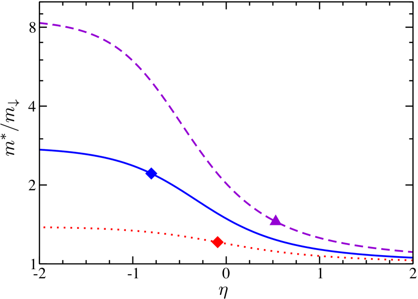
Figure 1: (Color online) Effective mass of the attractive polaron calculated within the variational ansatz $P_{3}$ as a function of interaction $\eta\equiv\ln(k_{F\uparrow}a_{2\rm{D}})$ for different mass ratios: $m_{\uparrow}/m_{\downarrow}$=6.64 (dashed), 1 (solid), 1/6.64 (dotted). For the equal mass case, our results match those obtained in Ref. Schmidt et al. (2012). The ground state is a polaron for weak attractive interactions but becomes a molecule (trimer) to the left of the diamond (triangle). Here we compare the wavefunction $P_{3}$ with $M_{4}$ and $T_{5}$, Eqs. (17) and (21).

In addition to the effective mass, the polarons are also described by the wave function overlap with the free impurity — the residue:

$$Z=\left|\alpha_{0}^{({\bf p})}\right|^{2}.$$ (16)

The residue of the attractive polaron goes to 1 in the limit $k_{F\uparrow}a_{2\rm{D}}\gg 1$ where the polaron is a well defined quasiparticle, while it vanishes in the opposite limit. The repulsive polaron displays the opposite behavior. We discuss the residue of the attractive polaron further in Sec. VI where we compare with the result of dressing the impurity by two particle-hole pair excitations.

The polaron state has been thoroughly studied in the 2D geometry. In particular, theoretical studies of $\left|{P_{3}}\right.\rangle$ have obtained the energy of the attractive polaron Zöllner et al. (2011); Parish (2011); the effective mass and residue of the attractive and repulsive polarons Schmidt et al. (2012); Ngampruetikorn et al. (2012); additionally, Ref. Ngampruetikorn et al. (2012) found the lowest lying repulsive polaron state in the limit $k_{F\uparrow}a_{2\rm{D}}\gg 1$ to have finite momentum. Experimental evidence of both the repulsive and the attractive polaron was found using radiofrequency spectroscopy in Ref. Koschorreck et al. (2012).

IV.2 Molecules ($M_{4}$)

We can likewise improve on the bare molecule state $\left|{M_{2}}\right.\rangle$ by adding one particle-hole pair as follows:

$$\left|{M_{4}({\mathbf{p}})}\right.\rangle =\sum_{{\mathbf{k}}}\varphi_{{\mathbf{k}}}^{({\mathbf{p}})}c^{\dagger}_{{\mathbf{p}}-{\mathbf{k}}\downarrow}c^{\dagger}_{{\mathbf{k}}\uparrow}\left|{FS}\right.\rangle$$

$$+\sum_{{\mathbf{k}}{\mathbf{k}^{\prime}}{\mathbf{q}}}\varphi_{{\mathbf{k}}{\mathbf{k}^{\prime}}{\mathbf{q}}}^{({\mathbf{p}})}c^{\dagger}_{{\mathbf{p}}+{\mathbf{q}}-{\mathbf{k}}-{\mathbf{k}^{\prime}}\downarrow}c^{\dagger}_{{\mathbf{k}}\uparrow}c^{\dagger}_{{\mathbf{k}^{\prime}}\uparrow}c_{{\mathbf{q}}\uparrow}\left|{FS}\right.\rangle.$$ (17)

The minimization procedure now leads to the following equations for the energy of the molecule:

$$\left[\frac{1}{g}+\sum_{{\bf k}}\frac{1}{E_{{\bf p}{\bf k}}}\right] =-\sum_{{\bf k}{\bf q}}\frac{G_{{\bf q}{\bf k}}}{E_{{\bf p}{\bf k}}},$$ (18)

$$\left[\frac{1}{g}+\sum_{{\bf k}}\frac{1}{E_{{\bf p}{\bf q}{\bf k}_{1}{\bf k}}}\right]G_{{\bf q}{\bf k}_{1}} =$$

$$\sum_{{\bf k}}\frac{G_{{\bf q}{\bf k}}}{E_{{\bf p}{\bf q}{\bf k}_{1}{\bf k}}} -\frac{1}{E_{{\bf p}{\bf k}_{1}}}-\sum_{{\bf q}^{\prime}}\frac{G_{{\bf q}^{\prime}{\bf k}_{1}}}{E_{{\bf p}{\bf k}_{1}}},$$ (19)

where $E_{{\bf p}{\bf k}}=-E+\xi_{{\bf k}\uparrow}+\epsilon_{{\bf p}+{\bf k}\downarrow}$ and $E_{{\bf p}{\bf q}{\bf k}_{1}{\bf k}_{2}}=-E+\xi_{{\bf k}_{1}\uparrow}+\xi_{{\bf k}_{2}\uparrow}-\xi_{{\bf q}\uparrow}+\epsilon_{{\bf p}+{\bf q}-{\bf k}_{1}-{\bf k}_{2}\downarrow}$. The function $G$ is defined as $G_{{\bf q}{\bf k}}\equiv\sum_{{\bf k}^{\prime}}\varphi^{({\bf p})}_{{\bf k}{\bf k}^{\prime}{\bf q}}/\sum_{{\bf k}^{\prime}}\varphi^{({\bf p})}_{{\bf k}^{\prime}}$. The energy of the molecule in the 2D geometry was first obtained in Ref. Parish (2011). The coupled integral equations (18) and (19) are equivalent to the equation for the molecule energy obtained in Refs. Combescot et al. (2009); Mora and Chevy (2009); Punk et al. (2009) for an impurity in a 3D Fermi gas.

Similarly to the polaron above, the energy of the molecule as a function of momentum yields the dispersion

$$E({\bf p})=E({\bf 0})+\frac{p^{2}}{2M^{*}},$$ (20)

with $M^{*}$ the effective mass. In the absence of interactions, the effective mass of the molecule is simply $M^{*}=m_{\uparrow}+m_{\downarrow}$. However, we observe a strong dependence of the effective mass on the interaction parameter, as shown in Fig. 2. As further illustrated in Fig. 3, once $M^{*}<0$ the molecule has its minimum energy at finite momentum, i.e. the pairing occurs at a finite momentum. As mentioned previously, this corresponds to the FFLO phase in the limit of large polarization, and we find that this phase occupies regions of the phase diagrams discussed in Sec. V.

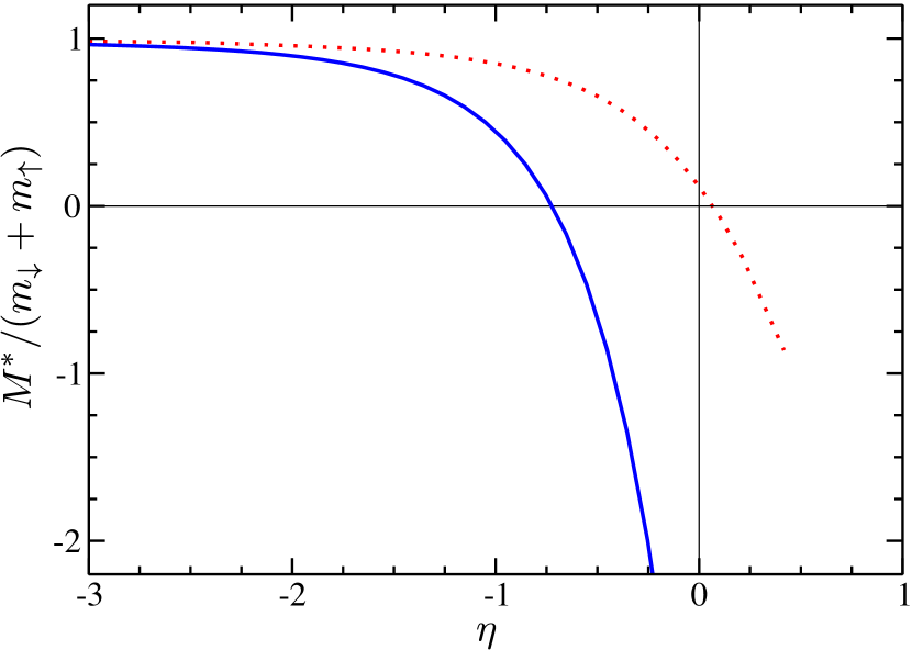
Figure 2: (Color online) Inverse effective mass of the molecule as a function of interaction parameter for different mass ratios: $m_{\uparrow}/m_{\downarrow}$= 1 (solid), 1/6.64 (dotted).

Figure 3: Illustration of the dispersion of $M_{4}({\bf p})$ for $m_{\uparrow}=2m_{\downarrow}$. (a) Momentum at the minimum of the dispersion as a function of interaction parameter. (b) Dispersion at $\eta=-1.25$ and (c) dispersion at $\eta=-1.1$.

IV.3 Trimers ($T_{5}$)

As discussed above, in the absence of a Fermi sea and for $r>3.33$, the impurity binds two particles to form a trimer. Since we wish to investigate the possibility of the trimer being the ground state across the regime of strong interactions, we use the dressed wave function

$$\left|{T_{5}({\bf 0})}\right.\rangle=\sum_{{\mathbf{k}_{1}}{\mathbf{k}_{2}}}\gamma_{{\mathbf{k}_{1}}{\mathbf{k}_{2}}}c^{\dagger}_{-{\mathbf{k}_{1}}-{\mathbf{k}_{2}}\downarrow}c^{\dagger}_{{\mathbf{k}_{1}}\uparrow}c^{\dagger}_{{\mathbf{k}_{2}}\uparrow}\left|{FS}\right.\rangle$$

$$+\sum_{{\mathbf{k}_{1}}{\mathbf{k}_{2}}{\mathbf{k}}{\mathbf{q}}}\gamma_{{\mathbf{k}_{1}}{\mathbf{k}_{2}}{\mathbf{k}}{\mathbf{q}}}c^{\dagger}_{{\mathbf{q}}-{\mathbf{k}_{1}}-{\mathbf{k}_{2}}-{\mathbf{k}}\downarrow}c^{\dagger}_{{\mathbf{k}_{1}}\uparrow}c^{\dagger}_{{\mathbf{k}_{2}}\uparrow}c^{\dagger}_{{\mathbf{k}}\uparrow}c_{{\mathbf{q}}\uparrow}\left|{FS}\right.\rangle.$$ (21)

Following the minimization procedure, we find two coupled integral equations:

$$J_{\mathbf{k}_{1}}\left[\frac{1}{g}+\sum_{{\mathbf{k}_{2}}}\frac{1}{E_{{\mathbf{k}_{1}}{\mathbf{k}_{2}}}}\right]=\sum_{{\bf k}_{2}}\frac{J_{\mathbf{k}_{2}}}{E_{{\mathbf{k}_{1}}{\mathbf{k}_{2}}}}-\sum_{{\mathbf{q}}{\bf k}_{2}}\frac{G_{{\bf q}{\bf k}_{1}{\bf k}_{2}}}{E_{{\mathbf{k}_{1}}{\mathbf{k}_{2}}}}$$ , (22)

$$G_{{\bf q}{\bf k}_{1}{\bf k}_{2}}\left[\frac{1}{g}+\sum_{{\bf k}}\frac{1}{E_{{\bf q}{\bf k}_{1}{\bf k}_{2}{\bf k}}}\right]=-\frac{J_{\mathbf{k}_{1}}-J_{\mathbf{k}_{2}}}{E_{{\mathbf{k}_{1}}{\mathbf{k}_{2}}}}$$

$$+\sum_{{\mathbf{k}}}\frac{G_{{\bf q}{\mathbf{k}_{1}}{\mathbf{k}}}+G_{{\bf q}{\mathbf{k}}{\mathbf{k}_{2}}}}{E_{{\bf q}{\mathbf{k}_{1}}{\mathbf{k}_{2}}{\mathbf{k}}}}-\sum_{{\mathbf{q}^{\prime}}}\frac{G_{{\bf q}^{\prime}{\bf k}_{1}{\bf k}_{2}}}{E_{{\mathbf{k}_{1}}{\mathbf{k}_{2}}}}$$ . (23)

We have defined $J_{\bf k}=g\sum_{{\mathbf{k}^{\prime}}}\gamma_{{\mathbf{k}}{\mathbf{k}^{\prime}}}$ and $G_{{\bf q}{\mathbf{k}_{1}}{\mathbf{k}_{2}}}=3g\sum_{{\mathbf{k}^{\prime}}}\gamma_{{\mathbf{k}_{1}}{\mathbf{k}_{2}}{\mathbf{k}^{\prime}}{\bf q}}$. The energies are $E_{{\mathbf{k}_{1}}{\mathbf{k}_{2}}}=-E+\xi_{{\bf k}_{1}\uparrow}+\xi_{{\bf k}_{2}\uparrow}+\epsilon_{{\mathbf{k}_{1}}+{\mathbf{k}_{2}}\downarrow}$ and $E_{{\bf q}{\mathbf{k}_{1}}{\mathbf{k}_{2}}{\mathbf{k}}}=-E+\xi_{{\bf k}_{1}\uparrow}+\xi_{{\bf k}_{2}\uparrow}+\xi_{{\bf k}\uparrow}-\xi_{{\bf q}\uparrow}+\epsilon_{{\bf q}-{\mathbf{k}}-{\mathbf{k}_{1}}-{\mathbf{k}_{2}}\downarrow}$. Eqs. (22) and (23) were first derived and solved for the trimer energy in Ref. Mathy et al. (2011) for the impurity problem in a 3D Fermi gas. The projection onto the $p$-wave trimer state is performed by taking

$$f_{{\bf k}_{1}}=\tilde{f}_{k_{1}}e^{i\phi_{1}},\hskip 11.38109ptG_{{\bf q}{\bf k}_{1}{\bf k}_{2}}=\tilde{G}(q,k_{1},k_{2},\Delta\phi_{1q},\Delta\phi_{2q})e^{i\phi_{1}},$$ (24)

with $\phi_{1}$, $\phi_{2}$, and $\phi_{q}$ the angles which ${\bf k}_{1}$, ${\bf k}_{2}$, and ${\bf q}$ make with the axis of reference, while $\Delta\phi_{1q}=\phi_{1}-\phi_{q}$ and $\Delta\phi_{2q}=\phi_{2}-\phi_{q}$.

IV.4 The $N+1$ problem

Like the bare wavefunctions of Sec. III, the above approach may be extended to the study of the bound states of the impurity and $N$ spin-$\uparrow$ fermions. The variational wave function is dressed by one particle-hole pair excitation of the Fermi sea and the minimization procedure carried out as above. This leads to two coupled integral equations similar to Eqs. (22) and (23) for the trimer above. The equations are derived in Appendix B using the diagrammatic technique. We shall not attempt here to solve for the energy of the tetramer or bound states containing even more particles.

V Phase diagrams

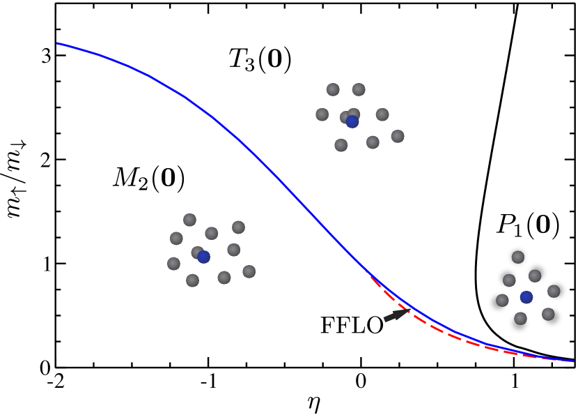
Figure 4: (Color online) Ground state phase diagram for an impurity atom attractively interacting with a 2D Fermi gas. The FFLO phase corresponds to the molecule $M_{2}({\mathbf{p}})$ with non-zero momentum ${\mathbf{p}}$ in the ground state. The behavior of the momentum at which the energy is at its minimum is given by Eq. (6) and it goes smoothly to zero at the dashed (red) line given by $m_{\uparrow}/m_{\downarrow}=1/(k_{F}a_{2\rm{D}})^{2}$. We find that small slivers of FFLO and trimer phases remain as $\eta\to\infty$. Note, also, that the trimer exists above the critical mass ratio $r\simeq 3.33$ in the limit $\eta\to-\infty$, which agrees with the result for the 3-body bound state in a vacuum Pricoupenko and Pedri (2010).

We now determine the ground state for the single impurity and the correponding binding transitions. In Fig. 4 we show the phase diagram for the “undressed” wave functions of Sec. III. Surprisingly, we find that a molecule existing at a given mass ratio $r<3.33$ must always first bind an extra spin-up fermion to form a trimer before it can unbind into a polaron. This appears to be an artifact of the approximation. However, it does signify the importance of three-body correlations for all mass ratios in 2D. Additionally, we find a sliver of FFLO phase, corresponding to a finite momentum molecule, on the border of the zero-momentum molecule and the trimer phases. The large region of trimer phase below $r\simeq 3.33$ appears to result from the fact that the FFLO molecule is unstable towards binding an extra $\uparrow$ particle, like in 3D Mathy et al. (2011). Whereas trimers are favored by the medium, we find that tetramers consisting of three spin-$\uparrow$ particles and the impurity appear to be disfavored, i.e. the phase transition is found to occur at larger mass ratios in the medium than the critical mass ratio of $r=5.0$ in vacuum Levinsen and Baur (2012). This suggests that four-body correlations are not as important in the many-body system at low mass ratios as might be initially expected.

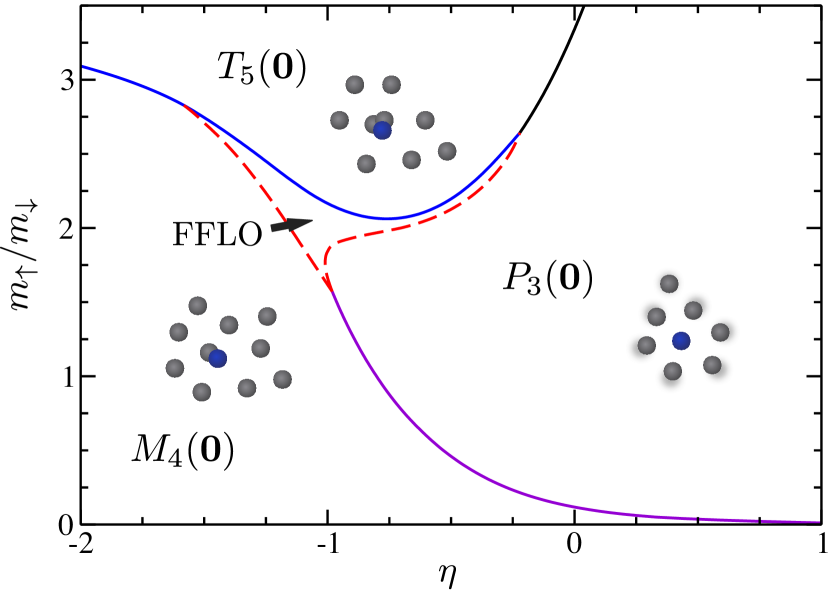
Figure 5: (Color online) Ground state phase diagram for a spin-down impurity atom immersed in a 2D Fermi gas, with phase boundaries calculated using the dressed wave functions of Sec. IV. The FFLO phase corresponds to the molecule $M_{4}({\mathbf{p}})$ with non-zero momentum ${\mathbf{p}}$ in the ground state. See Fig. 3 for the behavior of ${\mathbf{p}}$ as a function of $\eta$ across the FFLO region.

Next, Fig. 5 shows our phase diagram obtained using wave functions dressed by one particle-hole pair – see Sec. IV. As above, we find that the trimer is favored by the Fermi sea, but it now does not appear below a mass ratio of $r\approx 2.1$. Additionally, we find that the FFLO region, where the ground-state molecule has finite momentum, is enlarged at this level of approximation, making it possible that the FFLO phase may be observed in this system.

We expect this phase diagram to be qualitatively correct also across the regime of strong many-body corrections, $|1/\eta|\ll 1$, as contributions from two or more particle-hole pairs cancel approximately Combescot and Giraud (2008) and parts of the phase diagram are fixed by perturbative and exact calculations. In the limit of large negative $\eta$, the dressing of the molecule and trimer by one particle-hole pair yields the correct form of the first-order correction to their energy due to the interaction with the Fermi sea in a perturbative expansion in $1/|\eta|$. Thus the phase transition from $M_{4}({\bf 0})$ to $T_{5}({\bf 0})$ and the fact that the trimer is favored by the Fermi sea is quantitatively robust. Furthermore, for an impurity with infinite mass ($r=0$), the approach correctly identifies the dimer as the ground state Parish (2011).

VI Accuracy of the variational approach

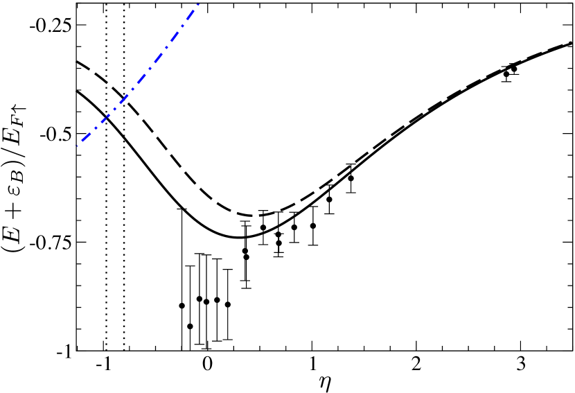
Figure 6: (Color online) Energy measured from the two-body binding energy. The dashed line corresponds to the results for the ansatz $\left|{P_{3}}\right.\rangle$, Eq. (11), the solid line to $\left|{P_{5}}\right.\rangle$, Eq. (LABEL:eq:p5), and the dot-dashed line to the molecule ansatz $\left|{M_{4}}\right.\rangle$, Eq. (17). The polaron-molecule transitions in the two approximations are illustrated by vertical dotted lines, while the experimental data is taken from Ref. Koschorreck et al. (2012), rescaled to reflect the quasi-2D nature of the experiment not (b).

The variational approach employed above has been validated by several methods in various settings. In 3D, the energy and effective mass of the attractive polaron quasiparticle have been measured in Refs. Schirotzek et al. (2009) and Nascimbène et al. (2009), respectively, and good agreement with the variational calculation Chevy (2006); Combescot et al. (2007) was obtained, even close to the unitary limit. It has also been shown that the polaron and molecule energies Combescot and Giraud (2008); Combescot et al. (2009); Mora and Chevy (2009); Punk et al. (2009) calculated using this method for a 3D Fermi gas with $m_{\uparrow}=m_{\downarrow}$ are in good agreement with those from quantum Monte Carlo Prokof’ev and Svistunov (2008a, b). More recently, an experimental and theoretical investigation of the population imbalanced ⁴⁰K-⁶Li mixture showed impressive agreement between the measured energies, residues, and lifetimes of the attractive and repulsive polarons when compared with the theoretical predictions from the diagrammatic technique Grimm (2011) (which is equivalent to the variational one presented here). Finally, it has been argued that contributions from two or more particle-hole excitations nearly cancel out via destructive interference Combescot and Giraud (2008). This argument does not depend on the dimension and indeed in the one-dimensional geometry it was shown that the variational ansatz agrees well with the exact Bethe Ansatz solution Giraud and Combescot (2009).

We now wish to demonstrate explicitly the accuracy of the dressed wave functions of the previous section. We emphasize the perturbative nature of the many-body system as long as $1/|\ln(k_{F\uparrow}a_{2\rm{D}})|\ll 1$, but we wish here to quantify the effect of quantum fluctuations in the strongly interacting region, $k_{F\uparrow}a_{2\rm{D}}\sim 1$. To this end we write down a variational wave function for the impurity dressed by two particle-hole pairs:

$$\left|{P_{5}({\bf 0})}\right.\rangle = \alpha_{0}c^{\dagger}_{{\mathbf{0}}\downarrow}\left|{FS}\right.\rangle+\sum_{{\mathbf{k}}{\mathbf{q}}}\alpha_{{\mathbf{k}}{\mathbf{q}}}c^{\dagger}_{{\mathbf{q}}-{\mathbf{k}}\downarrow}c^{\dagger}_{{\mathbf{k}}\uparrow}c_{{\mathbf{q}}\uparrow}\left|{FS}\right.\rangle$$ (27)

$$+\sum_{\tiny\begin{array}[]{c}{\bf k}_{1}{\bf k}_{2}\\ {\bf q}_{1}{\bf q}_{2}\end{array}}\alpha_{{\mathbf{k}_{1}}{\bf k}_{2}{\bf q}_{1}{\mathbf{q}_{2}}}c^{\dagger}_{{\mathbf{q}_{1}}+{\bf q}_{2}-{\mathbf{k}_{1}}-{\bf k}_{2}\downarrow}c^{\dagger}_{{\mathbf{k}_{1}}\uparrow}c^{\dagger}_{{\mathbf{k}_{2}}\uparrow}c_{{\mathbf{q}_{1}}\uparrow}c_{{\mathbf{q}_{2}}\uparrow}\left|{FS}\right.\rangle.$$

This wave function was first studied for the 3D polaron problem in Ref. Combescot and Giraud (2008). The minimization of $\langle\left.{P_{5}}\right|(H-E)\left|{P_{5}}\right.\rangle$ then results in two coupled integral equations,

$$f_{\bf q}\left[\frac{1}{g}+\sum_{\bf k}\frac{1}{E_{{\bf q}{\bf k}}}\right] = \sum_{{\bf q}^{\prime}}\frac{f_{{\bf q}^{\prime}}}{E}-\sum_{{\bf k}{\bf q}^{\prime}}\frac{G_{{\bf q}{\bf q}^{\prime}{\bf k}}}{E_{{\bf q}{\bf k}}},$$ (30)

$$G_{{\bf q}_{1}{\bf q}_{2}{\bf k}}\left[\frac{1}{g}+\sum_{{\bf k}^{\prime}}\frac{1}{E_{{\bf q}_{1}{\bf q}_{2}{\bf k}{\bf k}^{\prime}}}\right]=\sum_{{\bf k}^{\prime}}\frac{G_{{\bf q}_{1}{\bf q}_{2}{\bf k}^{\prime}}}{E_{{\bf q}_{1}{\bf q}_{2}{\bf k}{\bf k}^{\prime}}}$$

$$-\frac{f_{{\bf q}_{1}}+\sum_{{\bf q}_{2}^{\prime}}G_{{\bf q}_{1}{\bf q}_{2}^{\prime}{\bf k}}}{E_{{\bf q}_{1}{\bf k}}}+\frac{f_{{\bf q}_{2}}-\sum_{{\bf q}_{1}^{\prime}}G_{{\bf q}_{1}^{\prime}{\bf q}_{2}{\bf k}}}{E_{{\bf q}_{2}{\bf k}}}.$$

The energies are $E_{{\bf q}{\bf k}}=-E+\xi_{{\bf k}\uparrow}-\xi_{{\bf q}\uparrow}+\epsilon_{{\bf q}-{\bf k}\downarrow}$ and $E_{{\bf q}_{1}{\bf q}_{2}{\bf k}_{1}{\bf k}_{2}}=-E+\xi_{{\bf k}_{1}\uparrow}\xi_{{\bf k}_{2}\uparrow}-\xi_{{\bf q}_{1}\uparrow}-\xi_{{\bf q}_{2}\uparrow}+\epsilon_{{\bf q}_{1}+{\bf q}_{2}-{\bf k}_{1}-{\bf k}_{2}\downarrow}$, and we define $G_{{\bf q}_{1}{\bf q}_{2}{\bf k}}=4g\sum_{{\bf k}^{\prime}}\alpha_{{\bf k}^{\prime}{\bf k}{\bf q}_{1}{\bf q}_{2}}$ and $f_{\bf q}=g\sum_{\bf k}\alpha_{{\bf k}{\bf q}}$. The restriction to $s$-wave scattering of the impurity off a majority atom means that $f_{\bf q}$ depends only on the magnitude of ${\bf q}$. Likewise, the vertex $G$ depends on the magnitudes of ${\bf q}_{1}$, ${\bf q}_{2}$, and ${\bf k}$ and the two angles $\angle_{{\bf q}_{1},{\bf k}}$ and $\angle_{{\bf q}_{2},{\bf k}}$.

Our results for the polaron energy for equal masses of the two species are shown in Fig. 6. We see that the two ansätze agree very well in the weakly interacting regime, $\eta\gg 1$. In the regime of strong many-body effects, $1/|\eta|\ll 1$, the polaron energies resulting from the two ansätze show the same non-monotonic behavior and are never further separated than by 0.1$E_{F\uparrow}$. The polaron in a quasi-2D geometry was observed in a recent experiment Koschorreck et al. (2012). The data from the experiment is also displayed in Fig. 6 and is seen to match the energy of the $\left|{P_{5}}\right.\rangle$ ansatz quite well for $\eta\gtrsim 0.25$, leading us to believe that the $\left|{P_{5}}\right.\rangle$ ansatz is likely to closely reproduce the true energy of the polaron. The reason for the discrepancy below this value may be due to the finite interaction range of the interatomic potential, a finite density of impurity atoms, finite temperature effects, and trap-averaging effects.

From the polaron energies in the two ansätze we obtain the following values of the interaction parameter at the polaron-molecule transition:

$$P_{3}\mbox{-}M_{4}\mbox{ transition: } \ \eta=-0.80,\,\,\varepsilon_{B}/E_{F\uparrow}=9.9$$

$$P_{5}\mbox{-}M_{4}\mbox{ transition: } \ \eta=-0.97,\,\,\varepsilon_{B}/E_{F\uparrow}=14.0$$ (31)

This compares well with the experimental result of Koschorreck et al. Koe , $\eta=-0.88(0.20)$ not (b).

If the polaron and molecule variational wavefunctions converge with increasing numbers of particle-hole pair excitations, then it is possible to show that the above results for the polaron-molecule transition, Eq. (31), provide upper and lower bounds for the actual polaron-molecule transition. First, we define $E_{2n-1}-\varepsilon_{B}$ and $E_{2n}-\varepsilon_{B}$ to be the energies for the polaron $\left|{P_{2n-1}}\right.\rangle$ and molecule $\left|{M_{2n}}\right.\rangle$, respectively, with $n\geq 1$. Note that we must have $E_{2n+1}\leq E_{2n-1}$ and $E_{2n+2}\leq E_{2n}$ since larger $n$ corresponds to successively better variational wave functions with successively lower energies. Now we assume for each $\eta$ that the corrections to the energies become smaller with increasing $n$ such that

$$E_{2n+1}-E_{2n+3}\leq E_{2n}-E_{2n+2}\leq E_{2n-1}-E_{2n+1}$$ (32)

and we also assume that $E_{2n-1}$ ($E_{2n}$) is a monotonically decreasing (increasing) function of $\eta$ around the transition like in Fig. 6, i.e. near a given point $\eta_{0}$ we can write

$$E_{2n}(\eta) =E_{2n}(\eta_{0})+\rho_{M}(\eta-\eta_{0})$$

$$E_{2n-1}(\eta) =E_{2n-1}(\eta_{0})-\rho_{P}(\eta-\eta_{0})$$

where $\rho_{P},\rho_{M}>0$. Then for successively better approximations for the polaron-molecule transition:

$$E_{2n}(\eta^{+}) =E_{2n-1}(\eta^{+})$$

$$E_{2n}(\eta^{-}) =E_{2n+1}(\eta^{-})$$

$$E_{2n+2}(\eta^{\prime}) =E_{2n+1}(\eta^{\prime})$$

one can prove that $\eta^{-}<\eta^{\prime}<\eta^{+}$. Therefore the $P_{5}$-$M_{6}$ transition will lie between the $P_{5}$-$M_{4}$ and $P_{3}$-$M_{4}$ transitions, and so on, thus proving that the results (31) provide upper and lower bounds.

Finally, we also calculate the wavefunction overlap with the free impurity, the residue $Z$. As illustrated in Fig. 7, the residue also agrees quite well between the two ansätze, even across the regime of strong many-body effects. Note that the residue is finite at the polaron-molecule transition, indicating that the residue jumps to zero discontinously when the impurity binds an extra $\uparrow$ particle. This is a signature of a sharp “first-order” binding transition like in 3D Punk et al. (2009); Bruun and Massignan (2010). To our knowledge, our result for $\left|{P_{5}}\right.\rangle$ is the best estimate for the polaran residue thus far presented in the literature.

Figure 7: Residue of the attractive polaron for equal masses calculated from the variational wavefunctions $P_{5}({\bf 0})$ (solid line) and $P_{3}({\bf 0})$ (dashed). The dashed vertical lines represent the polaron-molecule transitions calculated within the two approximations.

VII Finite density

The high polarization limit of the phase diagram for the spin-imbalanced Fermi gas involves a finite density of impurities, and thus the question arises whether the single-impurity transitions are thermodynamically stable, i.e., whether they are preempted by first-order transitions in the thermodynamic limit. Typically, one requires the interactions between dressed impurities in order to assess this scenario; for instance, an attractive interaction between bosonic dressed impurities (e.g. dressed dimers or tetramers for a spin-down fermionic impurity atom) implies that the dressed impurities are unstable towards collapse into a region of higher density. However, the approach we will employ here is to determine whether the conditions for phase separation between the superfluid (SF) and fully-polarized normal (N) phases are ever satisfied. To this end, we assume that the superfluid is unpolarized and exploit the equal-mass equation of state for the BCS-BEC crossover derived from QMC calculations Bertaina and Giorgini (2011). This assumption is reasonable since no polarized superfluid is observed in the mean-field calculations for the 2D Fermi gas Conduit et al. (2008).

The onset of phase separation in a Fermi gas near full polarization corresponds to the following conditions for the pressures and chemical potentials in each phase:

$$p_{SF} =p_{N}\,,\ \ \mu^{SF}_{\sigma}=\mu^{N}_{\sigma}\,,\ \ \mu_{\downarrow}^{N}=E\,,$$ (33)

where $E$ is the energy of a single $\downarrow$ impurity immersed in a spin-polarized Fermi gas. At the mean-field level, this is very easily carried out by setting $E=0$, i.e. assuming that the impurity atom is non-interacting, and then analyzing the minima of the thermodynamic potential $\Omega(\Delta,\mu_{\sigma})\equiv-pV$, where $\Delta$ is the mean-field superfluid order parameter. Identifying the points at which we have degenerate minima at $\Delta=0$ and $\Delta\neq 0$ corresponds exactly to satisfying the conditions (33). Using the mean-field approach, we obtain a first-order transition at $\varepsilon_{B}/E_{F\uparrow}=\sqrt{1+r}-1$. Below, we obtain a more accurate result for the case of equal masses $m_{\uparrow}=m_{\downarrow}\equiv m$.

Clearly, the pressure and spin-up chemical potential in the fully-polarized normal phase are known exactly:

$$p_{N} =\frac{k_{F\uparrow}^{4}}{16\pi m}$$ (34)

$$\mu^{N}_{\uparrow} =\ E_{F\uparrow}=\frac{k_{F\uparrow}^{2}}{2m}$$ (35)

Thus, we just need to estimate the binding energy $E\equiv AE_{F\uparrow}$ to determine $\mu^{N}_{\downarrow}$. We obtain estimates from both wave functions $\left|{P_{3}}\right.\rangle$ and $\left|{P_{5}}\right.\rangle$.

The pressure and average chemical potential for the unpolarized superfluid can be written:

$$p_{SF} =\frac{k_{F}^{4}}{8\pi m}\zeta_{p}(\nu)$$ (36)

$$\mu^{SF} =\frac{\mu^{SF}_{\uparrow}+\mu^{SF}_{\downarrow}}{2}=\frac{k_{F}^{2}}{2m}\zeta_{\mu}(\nu)$$ (37)

where $\zeta_{p}(\nu)$, $\zeta_{\mu}(\nu)$ are interpolating functions that can be determined from the QMC equation of state Bertaina and Giorgini (2011), and $\nu=\ln(k_{F}a_{2\rm{D}})=\eta+\ln(k_{F}/k_{F\uparrow})$. The Fermi momentum $k_{F}$ of the superfluid is generally different from that in the fully-polarized phase.

By equating pressures and chemical potentials in each phase, we obtain the coupled equations

$$\left(\frac{k_{F\uparrow}}{k_{F}}\right)^{4}=2\zeta_{p}(\nu),\ \ \ \ \frac{k_{F\uparrow}}{k_{F}}=\sqrt{\frac{2\zeta_{\mu}(\nu)}{1+A}}$$ (38)

which must be solved for $\eta$ and $k_{F\uparrow}/k_{F}$. For the SF-N transition, we thus get within the two approximations for the impurity wave function

$$\left|{P_{3}}\right.\rangle:\ \ \ \eta=-0.69,\ \ \varepsilon_{B}/E_{F\uparrow}=7.9$$

$$\left|{P_{5}}\right.\rangle:\ \ \ \eta=-0.90,\ \ \varepsilon_{B}/E_{F\uparrow}=12.2$$ (39)

By comparing these values with (31), we see that this first-order transition (and the concomitant phase separation) preempts the single-impurity transition in the thermodynamic limit. This implies that the single-impurity transition effectively corresponds to a spinodal line for the SF-N transition, and this could be the case for much of the polaron-molecule transition line in Fig. 5. Note, however, that the results (39) strictly apply to zero temperature and require the existence of a superfluid. Such a SF-N transition may be destroyed by strong thermal fluctuations and so we can envisage a scenario where we only have the single-impurity transition existing at finite temperature. Future work is required to distinguish between these possible scenarios.

VIII Variational description of metastable states

The variational approach can also be generalized to study metastable excited states such as the repulsive polaron Schmidt et al. (2012); Ngampruetikorn et al. (2012); Cui and Zhai (2010); Massignan and Bruun (2011). Rather than minimizing the energy of the variational wave function, one instead needs to construct its equations of motion by minimizing the “error” quantity McLachlan (1964); Basile and Elser (1995)

$$\int\langle\left.{\psi(t)}\right|\delta^{\dagger}\delta\left|{\psi(t)}\right.\rangle dv$$

for all allowed variations of the unknown function $i\partial_{t}\psi(t)$, where $\delta=i\partial_{t}-H$. For the polaron wave function (11), this yields the same equations (12) and (13), but with energy $E$ replaced with $i\partial_{t}$. Now for a metastable polaron state with a long lifetime, we consider time-dependent amplitudes of the form $\alpha_{0}^{({\mathbf{p}})}(t)=\alpha_{0}^{({\mathbf{p}})}(0)e^{-iEt-\Gamma t}$ and $\alpha_{{\mathbf{k}}{\mathbf{q}}}^{({\mathbf{p}})}(t)=\alpha_{{\mathbf{k}}{\mathbf{q}}}^{({\mathbf{p}})}(0)e^{-iEt+\Gamma t}$, where the decay rate $\Gamma\ll|E|$. Note that we require $\alpha_{{\mathbf{k}}{\mathbf{q}}}^{({\mathbf{p}})}$ to grow exponentially with time while $\alpha_{0}^{({\mathbf{p}})}$ decreases exponentially so that the normalization condition $|\alpha_{0}^{({\mathbf{p}})}(t)|^{2}+\sum_{{\mathbf{k}}{\mathbf{q}}}|\alpha_{{\mathbf{k}}{\mathbf{q}}}^{({\mathbf{p}})}(t)|^{2}=1$ is preserved up to leading order in $\Gamma/E$. Inserting these amplitudes into the dynamical equations for the polaron then yields:

$$E-i\Gamma-\epsilon_{{\bf p}\downarrow} =\sum_{\bf q}\left[\frac{1}{g}+\sum_{\bf k}\frac{1}{E_{{\bf p}{\bf q}{\bf k}}-i\Gamma}\right]^{-1}$$

$$\equiv\Sigma({\mathbf{p}},E+i\Gamma)$$

which corresponds exactly to the condition for the quasiparticle pole within the diagrammatic approach Massignan and Bruun (2011). Thus, we obtain the usual equations for the energy and the decay rate of the repulsive polaron:

$$E =\epsilon_{{\bf p}\downarrow}+\Re[\Sigma({\mathbf{p}},E+i0)]$$

$$\Gamma \sim-\Im[\Sigma({\mathbf{p}},E+i0)]$$

In principle, this approach can also be used to study the metastable states proximate to the binding transitions Bruun and Massignan (2010). Note that energy and momentum conservation restricts the possible decay channels and means that a variational description which includes the metastability needs necessarily to include dressing by extra particle-hole pairs.

IX Concluding remarks

This work presents a thorough investigation of the highly polarized limit of a 2D Fermi gas, which can be modelled as a $\downarrow$ impurity in a $\uparrow$ Fermi sea. We have analyzed the possible states (polaron, molecule, trimer…) that the impurity can form and we have constructed the single-impurity phase diagram using two different levels of approximation for the impurity wave function. The simple “undressed” wave functions in Sec. III give us insight into the few-body correlations of the system and allow us to make contact with standard mean-field approaches for the spin-imbalanced Fermi gas. The wave functions dressed with one particle-hole excitation in Sec. IV contain the correct first-order correction to the impurity energy due to interactions with the medium, and they yield a phase diagram that should be qualitatively, if not quantitatively, accurate across the full range of interactions $\eta$. Indeed, our study of the polaron state with two particle-hole pairs in Sec. VI suggests that our variational approach is reasonable even in the regime of strong interactions $\eta\sim 0$. To better model experiment, the variational calculation may also be extended to properly include the transverse harmonic confinement — for further details, we refer the reader to Ref. Levinsen and Baur (2012).

Our results show that the trimer is strongly favored by the Fermi sea since the FFLO molecule is unstable to binding an extra $\uparrow$ fermion, like in 3D. However, there is still the possibility of observing the FFLO phase at lower mass ratios $1.8\lesssim r\lesssim 2.5$. A remaining question is what happens to the trimer phase when there is a finite density of impurities. Naively, one might expect a Fermi liquid of trimers if they are sufficiently tightly bound, but the fact that they have finite angular momentum could impact the properties of this liquid phase. There is also the question of whether the single-impurity binding transitions are thermodynamically stable — we have already shown that the polaron-molecule transition for equal masses is preempted by a SF-N transition at zero temperature. Such single-impurity transitions may nonetheless survive at finite temperature, in which case a finite density of molecules would correspond to a normal phase of preformed pairs.

Finally, we have computed rigorous upper and lower bounds for the position of the polaron-molecule transition in the case of equal masses. This should provide a useful benchmark for future experimental and theoretical work on this topic.

Appendix A Bound states in the $N+1$ problem

In this Appendix we demonstrate how the equations for the binding energy of a composite consisting of $N$ majority particles and 1 minority particle may be obtained by a diagrammatic technique. This is an alternative to the variational method described in the main text.

Consider first the undressed wavefunctions, the subject of Section III. For simplicity of notation, we will here consider the quasiparticle state at rest. The generalization to finite momentum may be easily achieved. The $\uparrow$ particles have momenta ${\bf k}_{1},\ldots,{\bf k}_{N}$ and corresponding energies $\xi_{{\bf k}_{1}\uparrow},\ldots,\xi_{{\bf k}_{N}\uparrow}$, while the impurity has momentum $-\sum_{i}{\bf k}_{i}$ and energy $E-\sum_{i}\xi_{{\bf k}_{i}\uparrow}$, such that the total energy is simply $E$.

The sum of diagrams with $N+1$ incoming particles where the impurity interacts first with the $\uparrow$ particle of momentum ${\bf k}_{1}$ will be denoted $f_{{\bf k}_{2}\ldots{\bf k}_{N}}$. The function $f$ does not depend on ${\bf k}_{1}$ since the initial interaction depends solely on the total momentum of the two particles. As the majority particles are fermions, $f$ is anti-symmetric in its indices. The specific ordering of indices is of course arbitrary, however once an ordering is chosen it must be kept throughout the calculation as this corresponds to a choice of ordering of operators in Wick’s theorem.

The occurence of an $N+1$ particle bound state with binding energy $E$ corresponds to a singularity of $f$ at this energy. For the polaron, $f$ is simply the bare impurity propagator and the energy is that of the non-interacting impurity. For the molecule, $f$ is the pair propagator in the medium, denoted $T_{2}$. For $N\geq 2$ the singularity appears from the summation of an infinite number of diagrams, and may be found by solving the integral equation illustrated in Fig. 8: The initial interaction between the impurity and the particle with momentum ${\bf k}_{1}$ is described by a pair propagator. Subsequently, the impurity interacts with another of the initial particles. Thus the right hand side contains $N-1$ terms and the function $f$ satisfies the integral equation

$$f_{{\bf k}_{2}\ldots{\bf k}_{N}}\left[\frac{1}{g}+\sum_{{\bf k}_{1}}\frac{1}{E_{{\bf k}_{1}\ldots{\bf k}_{N}}-i0}\right]=\sum_{{\bf k}_{1}}\frac{f_{{\bf k}_{1}{\bf k}_{3}\ldots{\bf k}_{N}}+f_{{\bf k}_{2}{\bf k}_{1}{\bf k}_{4}\ldots{\bf k}_{N}}+\ldots+f_{{\bf k}_{2}\ldots{\bf k}_{N-1}{\bf k}_{1}}}{E_{{\bf k}_{1}\ldots{\bf k}_{N}}-i0}.$$ (40)

where $E_{{\bf k}_{1}\ldots{\bf k}_{N}}=-E+\epsilon_{{\bf k}_{1}+\ldots+{\bf k}_{N}\downarrow}+\sum_{i}\xi_{{\bf k}_{i}\uparrow}$ and the factor $-i0$ acts to slightly shift the energy pole into the lower half of the complex plane. The quantity in brackets on the left hand side is the inverse pair propagator.

Appendix B The dressed $N+1$ problem

We turn now to the states dressed by one particle-hole excitation as investigated in Section IV. Again, we construct first the sum of all diagrams with $N$ incoming $\uparrow$ particles in which the impurity interacts first with the $\uparrow$ particle of momentum ${\bf k}_{1}$. The kinematics is chosen as above. Now we allow the vertex to be dressed by one particle hole pair and this new vertex is denoted $J_{{\bf k}_{2}\ldots{\bf k}_{N}}$. Again, the initial interaction is described through a pair propagator. Then, in addition to terms of the same form as above where the impurity interacts next with another of the initial particles, it may also interact next with a particle from the Fermi sea. This is illustrated in Fig. 9a where the sign arises from the fermion loop. The vertex $G_{{\bf q}{\bf k}_{1}\ldots{\bf k}_{N}}$ is the sum of all diagrams with one incoming $\downarrow$ particle and $N+1$ incoming $\uparrow$ particles, the initial interaction being between the impurity and the particle having momentum ${\bf q}$ and energy $\xi_{{\bf q}\uparrow}$. The equation in Fig. 9a is

$$J_{{\bf k}_{2}\ldots{\bf k}_{N}}\left[\frac{1}{g}+\sum_{{\bf k}_{1}}\frac{1}{E_{{\bf k}_{1}\ldots{\bf k}_{N}}-i0}\right]=\sum_{{\bf k}_{1}}\frac{J_{{\bf k}_{1}{\bf k}_{3}\ldots{\bf k}_{N}}+J_{{\bf k}_{2}{\bf k}_{1}{\bf k}_{4}\ldots{\bf k}_{N}}+\ldots+J_{{\bf k}_{2}\ldots{\bf k}_{N-1}{\bf k}_{1}}}{E_{{\bf k}_{1}\ldots{\bf k}_{N}}-i0}-\sum_{{\bf k}_{1}{\bf q}}\frac{G_{{\bf q}{\bf k}_{1}\ldots{\bf k}_{n}}}{E_{{\bf k}_{1}\ldots{\bf k}_{n}}-i0}.$$ (41)

Figure 8: The diagrams which lead to the binding energy of the $N+1$ composite. Black dots on vertices indicate that the corresponding particles interact first inside the vertex $f$.

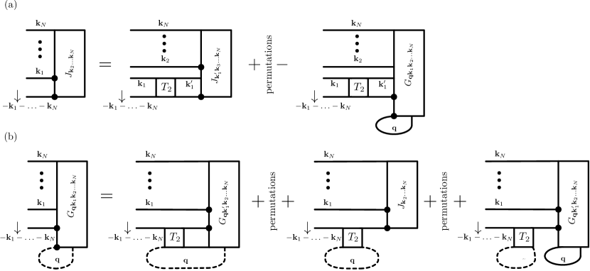
Figure 9: The equations which give the binding energy of the $N+1$ composite including dressing by one particle-hole pair. Black dots on vertices indicate that the corresponding particles interact first inside the vertex. (a) The equation for the vertex $J$, there are $N-1$ diagrams of the first type on the r.h.s. corresponding to interactions between the impurity and one of the particles with momentum ${\bf k}_{2},\ldots,{\bf k}_{N}$ and 1 of the second type. (b) The equation for $G$. The first two types of diagrams on the r.h.s. appear $N$ times corresponding to interactions between the impurity and one of the particles with momentum ${\bf k}_{1},\ldots,{\bf k}_{N}$. Dashed lines indicate that these are the loops which are closed upon insertion of $G$ in the diagrams in (a).

The vertex $G$ is constructed as follows: The initial interaction between the impurity and the particle with momentum ${\bf q}$ is again described by a pair propagator. After this interaction, the $\uparrow$ particle which partakes in this repeated interaction is either disconnected or connected from the remaining particles. If it is connected then the impurity interacts next with one of the particles with momentum ${\bf k}_{1},\ldots,{\bf k}_{N}$, as the vertex is only dressed by one particle hole pair. This interaction is again described by the vertex $G$. If disconnected, the impurity can interact first with one of the particles with momentum ${\bf k}_{1},\ldots,{\bf k}_{N}$ and this interaction is given by the vertex $J$, or it can interact first with a particle from the Fermi sea. This results in the equation for $G$:

$$G_{{\bf q}{\bf k}_{1}\ldots{\bf k}_{N}}\left[\frac{1}{g}+\sum_{{\bf k}}\frac{1}{E_{{\bf q}{\bf k}_{1}\ldots{\bf k}_{N}{\bf k}}-i0}\right] = \sum_{{\bf k}}\frac{G_{{\bf q}{\bf k}{\bf k}_{2}\ldots{\bf k}_{N}}+G_{{\bf q}{\bf k}_{1}{\bf k}{\bf k}_{3}\ldots{\bf k}_{N}}+\ldots+G_{{\bf q}{\bf k}_{1}\ldots{\bf k}_{N-1}{\bf k}}}{E_{{\bf q}{\bf k}_{1}\ldots{\bf k}_{N}{\bf k}}-i0}$$ (42)

$$-\frac{J_{{\bf k}_{2}\ldots{\bf k}_{N}}-J_{{\bf k}_{1}{\bf k}_{3}\ldots{\bf k}_{N}}+J_{{\bf k}_{1}{\bf k}_{2}{\bf k}_{4}\ldots{\bf k}_{N}}-\ldots+(-1)^{N-1}J_{{\bf k}_{1}\ldots{\bf k}_{N-1}}}{E_{{\bf k}_{1}\ldots{\bf k}_{N}}-i0}-\frac{\sum_{{\bf q}^{\prime}}G_{{\bf q}^{\prime}{\bf k}_{1}\ldots{\bf k}_{N}}}{E_{{\bf k}_{1}\ldots{\bf k}_{N}}-i0},$$

where $E_{{\bf q}{\bf k}_{1}\ldots{\bf k}_{N}{\bf k}}=-E+\epsilon_{{\bf q}-{\bf k}_{1}\ldots-{\bf k}_{N}-{\bf k}\downarrow}+\sum_{i}\xi_{{\bf k}_{i}\uparrow}+\xi_{{\bf k}\uparrow}-\xi_{{\bf q}\uparrow}$. Eq. (42) is illustrated in Fig. 9b where the dotted lines, indicating how the loops are closed, should only be taken as a guide to the eye, as the integration over momentum in these loops is not performed until the insertion of this equation in Eq. (41).

References

- Martiyanov et al. (2010) K. Martiyanov, V. Makhalov, and A. Turlapov, Phys. Rev. Lett. 105, 030404 (2010).
- Fröhlich et al. (2011) B. Fröhlich, M. Feld, E. Vogt, M. Koschorreck, W. Zwerger, and M. Köhl, Phys. Rev. Lett. 106, 105301 (2011).
- Dyke et al. (2011) P. Dyke, E. D. Kuhnle, S. Whitlock, H. Hu, M. Mark, S. Hoinka, M. Lingham, P. Hannaford, and C. J. Vale, Phys. Rev. Lett. 106, 105304 (2011).
- Feld et al. (2011) M. Feld, B. Fröhlich, E. Vogt, M. Koschorreck, and M. Köhl, Nature (London) 480, 75 (2011).
- Sommer et al. (2012) A. T. Sommer, L. W. Cheuk, M. J. H. Ku, W. S. Bakr, and M. W. Zwierlein, Phys. Rev. Lett. 108, 045302 (2012).
- Koschorreck et al. (2012) M. Koschorreck, D. Pertot, E. Vogt, B. Fröhlich, M. Feld, and M. Köhl, Nature (London) 485, 619 (2012).
- Zhang et al. (2012) Y. Zhang, W. Ong, I. Arakelyan, and J. E. Thomas, Phys. Rev. Lett. 108, 235302 (2012).
- Croxall et al. (2008) A. F. Croxall, K. Das Gupta, C. A. Nicoll, M. Thangaraj, H. E. Beere, I. Farrer, D. A. Ritchie, and M. Pepper, Phys. Rev. Lett. 101, 246801 (2008).
- Seamons et al. (2009) J. A. Seamons, C. P. Morath, J. L. Reno, and M. P. Lilly, Phys. Rev. Lett. 102, 026804 (2009).
- Norman (2011) M. R. Norman, Science 332, 196 (2011).
- Fröhlich (1954) H. Fröhlich, Advances in Physics 3, 325 (1954).
- Prokof’ev and Svistunov (2008a) N. Prokof’ev and B. Svistunov, Phys. Rev. B 77, 020408 (2008a).
- Prokof’ev and Svistunov (2008b) N. V. Prokof’ev and B. V. Svistunov, Phys. Rev. B 77, 125101 (2008b).
- Parish et al. (2007a) M. M. Parish, F. M. Marchetti, A. Lamacraft, and B. D. Simons, Nature Phys. 3, 124 (2007a).
- Sheehy and Radzihovsky (2007) D. E. Sheehy and L. Radzihovsky, Annals of Physics 322, 1790 (2007).
- Chevy (2006) F. Chevy, Phys. Rev. A 74, 063628 (2006).
- Combescot et al. (2009) R. Combescot, S. Giraud, and X. Leyronas, Europhys. Lett. 88, 60007 (2009).
- Mora and Chevy (2009) C. Mora and F. Chevy, Phys. Rev. A 80, 033607 (2009).
- Punk et al. (2009) M. Punk, P. T. Dumitrescu, and W. Zwerger, Phys. Rev. A 80, 053605 (2009).
- Mathy et al. (2011) C. J. M. Mathy, M. M. Parish, and D. A. Huse, Phys. Rev. Lett 106, 166404 (2011).
- Zöllner et al. (2011) S. Zöllner, G. M. Bruun, and C. J. Pethick, Phys. Rev. A 83, 021603(R) (2011).
- Klawunn and Recati (2011) M. Klawunn and A. Recati, Phys. Rev. A 84, 033607 (2011).
- Parish (2011) M. M. Parish, Phys. Rev. A 83, 051603 (2011).
- Levinsen and Baur (2012) J. Levinsen and S. K. Baur, Phys. Rev. A 86, 041602 (2012).
- Pricoupenko and Pedri (2010) L. Pricoupenko and P. Pedri, Phys. Rev. A 82, 033625 (2010).
- Levinsen and Parish (2012) J. Levinsen and M. M. Parish, arXiv:1207.0459 (2012).
- Fulde and Ferrell (1964) P. Fulde and R. A. Ferrell, Phys. Rev. 135, A550 (1964).
- Larkin and Ovchinnikov (1967) A. I. Larkin and Y. N. Ovchinnikov, Soviet JETP 20, 762 (1967).
- Levinsen et al. (2009) J. Levinsen, T. G. Tiecke, J. T. M. Walraven, and D. S. Petrov, Phys. Rev. Lett. 103, 153202 (2009).
- Ngampruetikorn et al. (2012) V. Ngampruetikorn, M. M. Parish, and J. Levinsen, arXiv:1211.6805 (2012).
- Combescot et al. (2007) R. Combescot, A. Recati, C. Lobo, and F. Chevy, Phys. Rev. Lett. 98, 180402 (2007).
- Bertaina and Giorgini (2011) G. Bertaina and S. Giorgini, Phys. Rev. Lett. 106, 110403 (2011).
- Landau and Lifshitz (1981) L. D. Landau and E. M. Lifshitz, Quantum Mechanics (Butterworth-Heinemann, Oxford, UK, 1981).
- Bloom (1975) P. Bloom, Phys. Rev. B 12, 125 (1975).
- Parish et al. (2007b) M. M. Parish, F. M. Marchetti, A. Lamacraft, and B. D. Simons, Phys. Rev. Lett. 98, 160402 (2007b).
- Delves and Mohamed (1985) L. M. Delves and J. L. Mohamed, Computational methods for integral equations (Cambridge University Press, 1985).
- Castin et al. (2010) Y. Castin, C. Mora, and L. Pricoupenko, Phys. Rev. Lett. 105, 223201 (2010).
- Minlos (1995) R. Minlos, in Proceedings of the Workshop on Singular Schrödinger Operators, Trieste, 29 September-1 October 1994, edited by G. Dell’Antonio, R. Figari, and A. Teta (SISSA, Trieste, 1995).
- not (a) Note, however, that the factor in Eq. (10) of Ref. Minlos (1995) should be squared.
- Pricoupenko (2011) L. Pricoupenko, Phys. Rev. A 83, 062711 (2011).
- Combescot and Giraud (2008) R. Combescot and S. Giraud, Phys. Rev. Lett. 101, 050404 (2008).
- Schmidt et al. (2012) R. Schmidt, T. Enss, V. Pietilä, and E. Demler, Phys. Rev. A 85, 021602 (2012).
- Ngampruetikorn et al. (2012) V. Ngampruetikorn, J. Levinsen, and M. M. Parish, Europhys. Lett. 98, 30005 (2012).
- not (b) In the experimental work of Ref. Koschorreck et al. (2012), the definition is used to relate the binding energy to . However, in a quasi-2D geometry it is necessary to take into account the, approximately harmonic, confining potential in the -direction in order to obtain the 2D scattering length characterising the low-energy scattering: , with , and Petrov and Shlyapnikov (2001); Bloch et al. (2008). As argued in Ref. Levinsen and Baur (2012), this latter definition of yields a better agreement between the quasi-2D experiments and the strict 2D theory employed in the present work.
- Schirotzek et al. (2009) A. Schirotzek, C.-H. Wu, A. Sommer, and M. W. Zwierlein, Phys. Rev. Lett. 102, 230402 (2009).
- Nascimbène et al. (2009) S. Nascimbène, N. Navon, K. J. Jiang, L. Tarruell, M. Teichmann, J. McKeever, F. Chevy, and C. Salomon, Phys. Rev. Lett. 103, 170402 (2009).
- Grimm (2011) R. Grimm, talk at BEC 2011, Sant Feliu (2011).
- Giraud and Combescot (2009) S. Giraud and R. Combescot, Phys. Rev. A 79, 043615 (2009).
- (49) M. Köhl, talk at the 2012 APS March meeting.
- Bruun and Massignan (2010) G. M. Bruun and P. Massignan, Phys. Rev. Lett. 105, 020403 (2010).
- Conduit et al. (2008) G. J. Conduit, P. H. Conlon, and B. D. Simons, Phys. Rev. A 77, 053617 (2008).
- Cui and Zhai (2010) X. Cui and H. Zhai, Phys. Rev. A 81, 041602 (2010).
- Massignan and Bruun (2011) P. Massignan and G. M. Bruun, Eur. Phys. J. D (2011).
- McLachlan (1964) A. D. McLachlan, Molecular Physics 8, 39 (1964).
- Basile and Elser (1995) A. G. Basile and V. Elser, Phys. Rev. E 51, 5688 (1995).
- Petrov and Shlyapnikov (2001) D. S. Petrov and G. V. Shlyapnikov, Phys. Rev. A 64, 012706 (2001).
- Bloch et al. (2008) I. Bloch, J. Dalibard, and W. Zwerger, Rev. Mod. Phys. 80, 885 (2008).