The existence of a bending rigidity for a hard sphere liquid

near a curved hard wall: Helfrich or Hadwiger?

Edgar M. Blokhuis

Colloid and Interface Science, Leiden Institute of Chemistry,

Gorlaeus Laboratories, P.O. Box 9502, 2300 RA Leiden, The Netherlands.

Abstract

In the context of Rosenfeld’s Fundamental Measure Theory, we show that the bending rigidity is not equal to zero for a hard-sphere fluid in contact with a curved hard wall. The implication is that the Hadwiger Theorem does not hold in this case and the surface free energy is given by the Helfrich expansion instead. The value obtained for the bending rigidity is (1) an order of magnitude smaller than the bending constant associated with Gaussian curvature, (2) changes sign as a function of the fluid volume fraction, (3) is independent of the choice for the location of the hard wall.

 

I Introduction

The Helfrich free energy Helfrich has proven to be an invaluable starting point in the description of the surface properties of complex surfaces such as membranes or surfactant systems surfactants ; Safran . It is the most general form for the surface (or excess) free energy of an isotropic surface expanded to second order in the surface’s curvature:

$$\Omega_{\rm H}=\int\!\!dA\;[\,\sigma-\delta\sigma\,J+\frac{k}{2}\,J^{2}+\bar{k}\,K\,+\ldots]\,,$$ (1)

where $J\!=\!1/R_{1}+1/R_{2}$ is the total curvature, $K\!=\!1/(R_{1}R_{2})$ is the Gaussian curvature and $R_{1}$, $R_{2}$ are the principal radii of curvature at a certain point on the surface. The expansion defines four curvature coefficients: $\sigma$, the surface tension of the planar interface, $\delta$, the Tolman length Tolman , $k$, the bending rigidity, and $\bar{k}$, the rigidity constant associated with Gaussian curvature. The original expression proposed by Helfrich Helfrich features the radius of spontaneous curvature $R_{0}$ as the linear curvature term ($\delta\sigma\rightarrow 2k/R_{0}$ Blokhuis92 ; Blokhuis06 ), but in honour of Tolman, who was the first to consider curvature corrections to the surface tension Tolman , we use the notation in Eq.(1).

Recently, an alternative description to replace the Helfrich free energy in certain situations was put forward by König et al. Konig04 ; Konig05 based on the implications of the Hadwiger Theorem Hadwiger ; Mecke . The Hadwiger Theorem states that any functional of a system that is translationally invariant, additive and continuous, can be written as a linear combination of the four Minkowski functionals: volume, surface area, and the integrated total and Gaussian curvatures Mecke . The implication is that, as an alternative to Eq.(1), the surface free energy can be written as:

$$\Omega_{\rm Hadwiger}=\int\!\!dA\;[\,\sigma-\delta\sigma\,J+\bar{k}\,K]\,.$$ (2)

Comparing the two expressions for the free energy in Eqs.(1) and (2), we are led to the following two implications of the Hadwiger Theorem:
1. The bending rigidity constant is zero,
2. Higher order curvature terms, represented by the dots in Eq.(1), are absent.

The question now is for which systems are the conditions of the Hadwiger Theorem fulfilled so that the bending rigidity and higher order curvature terms are all strictly zero? It was suggested that for a hard sphere fluid in contact with a hard, structureless wall, the Hadwiger Theorem should hold and Eq.(2) is a complete expression for its surface free energy Konig04 ; Konig05 . The evidence for this suggestion is based on a numerical analysis Konig04 ; Konig05 ; Bryk03 of the free energy in spherical and cylindrical geometry using Rosenfeld’s Fundamental Measure Theory (FMT) Rosenfeld ; Roth , showing that the bending rigidity is zero within numerical accuracy. To understand the basis for this result in more detail, we consider surfaces for which the curvatures $J$ and $K$ are constant. The Helfrich free energy per unit area is then given by:

$$\Omega_{\rm H}/A\equiv\sigma(J,K)=\sigma-\delta\sigma\,J+\frac{k}{2}\,J^{2}+\bar{k}\,K+\ldots$$ (3)

For a spherically or cylindrically shaped surface with radius $R$, this expansion then takes the form:

$$\sigma_{s}(R) = \sigma-\frac{2\delta\sigma}{R}+\frac{(2k+\bar{k})}{R^{2}}+\ldots\hskip 27.0pt{\rm(sphere)}$$ (4)

$$\sigma_{c}(R) = \sigma-\frac{\delta\sigma}{R}+\frac{k}{2R^{2}}+\ldots\hskip 56.0pt{\rm(cylinder)}$$ (5)

Note that only the combination $2k+\bar{k}$ appears in the expression for the surface tension of the spherical interface, so that the conclusion whether $k$ is identically zero or not can be made only from an analysis of the cylindrical system. Next to the curvature dependent surface tension, one may also investigate the curvature dependence of the wall density $\rho^{\rm W}$. According to the wall theorem, the wall density of a fluid in contact with an infinitely hard, planar wall is related to the bulk pressure $p$ through an ideal gas law Lebowitz ; Henderson83 :

$$k_{\rm B}T\,\rho^{\rm W}=p\,.$$ (6)

The wall theorem can be generalized to a spherically shaped hard wall Henderson83 ; Henderson86 ; Blokhuis07 or to a more generally shaped hard wall with (constant) curvatures $J$ and $K$ Blokhuis_unpublished :

$$k_{\rm B}T\,\rho^{\rm W}(J,K)=p+\sigma\,J-2\delta\sigma\,K-\frac{k}{2}\,J^{3}+2k\,J\,K+\ldots$$ (7)

Note that a term proportional to $J^{2}$ is absent in the expression above Note . For a spherically or cylindrically shaped surface, this expansion takes the form:

$$k_{\rm B}T\,\rho_{s}^{\rm W}(R) = p+\frac{2\sigma}{R}-\frac{2\delta\sigma}{R^{2}}+\dots\hskip 40.0pt{\rm(sphere)}$$ (8)

$$k_{\rm B}T\,\rho_{c}^{\rm W}(R) = p+\frac{\sigma}{R}-\frac{k}{2R^{3}}+\dots\hskip 43.0pt{\rm(cylinder)}$$ (9)

where the dots represent terms of ${\cal O}(1/R^{4})$ which indicates that the term proportional to $1/R^{3}$ is absent in the expansion of the spherical interface. The corresponding term in the expansion of the cylindrical interface is related to the bending rigidity thus supplying a second route to the determination of its value. Note that these expressions are valid only when the radius $R$ is defined via the wall density $\rho^{\rm W}\!\equiv\!\rho(r\!=\!R^{+})$.

In this article, we revisit the analysis by König et al. Konig04 ; Konig05 for a hard sphere fluid in contact with a hard wall. Using the exact same theoretical model as in refs. Konig04 ; Konig05 ; Bryk03 , i.e. FMT Rosenfeld ; Roth , we show in Section II that a detailed numerical analysis yields a bending rigidity that is not equal to zero, but an order of magnitude smaller than the rigidity constant associated with Gaussian curvature. Consistent values for $k$ are obtained from the analysis of the radius dependence of the surface tension, Eq.(5), as well as from the analysis of the radius dependence of the wall density, Eq.(9).

As a further consistency test, we perform a systematic expansion of the FMT free energy to second order in the curvature for the spherical and cylindrical interface in Section III. This expansion is analogous to a similar expansion for the liquid-vapour interface Blokhuis93 . It is shown that the resulting expressions for $\sigma$, $\delta$, and $\bar{k}$ are all in terms of the fluid density profile of the planar interface, $\rho_{0}(z)$, whereas the expression for the bending rigidity $k$, features the leading order curvature correction to the density profile, $\rho_{1}(z)$. The values obtained for $\sigma$, $\delta\sigma$, and the combination $2k+\bar{k}$ using these expressions are all consistent with the results of König et al. Konig04 ; Konig05 and those by Bryk et al. Bryk03 . The value obtained for the bending rigidity is not zero and consistent with the two values obtained from the radius dependent surface tension and wall density. Furthermore, it is in qualitative agreement with recent MD simulations by Laird et al. Laird12 who determined the curvature dependent surface tension of a fluid near a hard wall by Gibbs-Cahn integration Laird12 ; Laird10 .

II Fundamental measure theory

In this section, we discuss Rosenfeld’s Fundamental Measure Theory Rosenfeld as it is applied specifically to a one-component fluid consisting of spherical particles with a diameter $d$. The free energy is then the following functional of the fluid density $\rho(\vec{r})$ Rosenfeld ; Roth :

$$\frac{\Omega[\rho]}{k_{\rm B}T}=\int\!\!d\vec{r}\;\left[\rho\,\ln(\rho)-\rho-\frac{\mu}{k_{\rm B}T}\,\rho+\frac{V_{\rm ext}(\vec{r})}{k_{\rm B}T}\,\rho+\phi\right]\,,$$ (10)

where $\mu$ is the chemical potential and where the external field $V_{\rm ext}(\vec{r})$ is used to express the presence of the hard wall. For spherically shaped fluid particles the free energy density $\phi\!=\!\phi(n_{2},n_{3},\vec{n}_{V})$ is explicitly given by

$$\phi=\frac{1}{\pi d^{2}}\left[-n_{2}\,\ln(1-n_{3})+\frac{d^{2}(n_{2}^{2}-|\vec{n}_{\rm V}|^{2})}{2(1-n_{3})}+\frac{d^{2}(n_{2}^{3}-3n_{2}\,|\vec{n}_{\rm V}|^{2})}{24(1-n_{3})^{2}}\right]\,.$$ (11)

The three densities $n_{\alpha}(\vec{r})$ ($\alpha\!=\!2,3,V$) are different convolutions of the fluid density

$$n_{\alpha}(\vec{r}_{1})=\int\!\!d\vec{r}_{2}\;\rho(\vec{r}_{2})\,w_{\alpha}(\vec{r}_{1}-\vec{r}_{2})\,,$$ (12)

where the weight functions $w_{\alpha}(\vec{r})$ are explicitly given by Roth

$$w_{2}(\vec{r})=\delta(\frac{d}{2}-r)\,,\hskip 30.0ptw_{3}(\vec{r})=\Theta(\frac{d}{2}-r)\hskip 20.0pt{\rm and}\hskip 20.0pt\vec{w}_{\rm V}(\vec{r})=\frac{\vec{r}}{r}\,\delta(\frac{d}{2}-r)\,.$$ (13)

The Euler-Lagrange equation that minimizes the free energy in Eq.(10) is given by

$$\frac{\mu}{k_{\rm B}T}=\ln(\rho)+\frac{V_{\rm ext}(\vec{r})}{k_{\rm B}T}+\sum\limits_{\alpha}\int\!\!d\vec{r}_{2}\;\frac{\partial\phi}{\partial n_{\alpha}(\vec{r}_{2})}\,w_{\alpha}(\vec{r}_{2}-\vec{r}_{1})\,.$$ (14)

Note that the Euler-Lagrange equation features $w_{\alpha}(\vec{r}_{2}-\vec{r}_{1})$ and not $w_{\alpha}(\vec{r}_{1}-\vec{r}_{2})$ as in Eq.(12) Roth .

For a uniform system, we have that $n_{2}\!=\!6\eta/d$, $n_{3}\!=\!\eta$ and $\vec{n}_{\rm V}\!=\!0$, with the volume fraction defined as $\eta\!\equiv\!(\pi/6)\,\rho\,d^{3}$. The Euler-Lagrange equation in Eq.(14) then becomes:

$$\frac{\mu}{k_{\rm B}T}=\ln(\rho)-\ln(1-\eta)+\frac{\eta\,(14-13\eta+5\eta^{2})}{2(1-\eta)^{3}}\,.$$ (15)

Using the expression for the chemical potential above the bulk pressure is obtained from $\Omega\!=\!-pV$ giving the Percus-Yevick equation of state:

$$\frac{d^{3}\,p}{k_{\rm B}T}=\frac{6\eta\,(1+\eta+\eta^{2})}{\pi(1-\eta)^{3}}\,.$$ (16)

We mention that a refinement of FMT was recently proposed FMT_CS to yield the more accurate Carnahan Starling equation of state CS instead of Eq.(16). It is expected that results do not depend sensitively on this refinement.

Next, we consider the implementation of FMT in three different geometries: the planar, spherical, and cylindrical interface. Planar interface In planar geometry, we can simplify the expressions for $n_{\alpha}(\vec{r})\!=\!n_{\alpha}(z)$, where $z$ is the coordinate normal to the interface, as:

$$n_{\alpha}(z_{1})=\int\!\!dz_{2}\;\rho(z_{2})\,w^{0}_{\alpha}(z_{1}-z_{2})\,,$$ (17)

where the weight functions $w^{0}_{\alpha}(z)$ are explicitly given by

$$w^{0}_{2}(z) = \pi d\,\Theta(\frac{d}{2}-|z|)\,,$$ (18)

$$w^{0}_{3}(z) = \pi(\frac{d^{2}}{4}-z^{2})\,\Theta(\frac{d}{2}-|z|)\,,$$

$$w^{0}_{\rm V}(z) = 2\pi z\,\Theta(\frac{d}{2}-|z|)\,,$$

and where $\vec{n}_{\rm V}(\vec{r})\!=\!n_{\rm V}(z)\hat{z}$. The Euler-Lagrange equation in Eq.(14) simplifies in planar geometry to

$$\frac{\mu}{k_{\rm B}T}=\ln(\rho)+\frac{V_{\rm ext}(z_{1})}{k_{\rm B}T}+\sum\limits_{\alpha}\int\!\!dz_{2}\;\frac{\partial\phi}{\partial n_{\alpha}(z_{2})}\,w^{0}_{\alpha}(z_{2}-z_{1})\,.$$ (19)

The external field mimics the presence of a hard wall for $z\!<\!0$, i.e. $V_{\rm ext}(z)\!=\!\infty$ when $z<0$ and zero otherwise, so that the density $\rho(z)\!=\!0$ for $z\!<\!0$. The surface tension is the surface free energy per unit area ($\sigma\!=\!(\Omega+p\,V)/A$ RW ):

$$\frac{\sigma}{k_{\rm B}T}=\int\limits_{-d/2}^{\infty}\!\!\!\!\!dz\left[\rho\,\ln(\rho)-\rho-\frac{\mu}{k_{\rm B}T}\,\rho+\phi+\frac{p}{k_{\rm B}T}\,\Theta(z)\right]\,,$$ (20)

where the lower integration reflects the fact that $\phi$ and the convoluted densities $n_{\alpha}(z)$ are zero only when $z\!<\!-d/2$. Spherical interface In spherical geometry, the densities $n_{\alpha}(\vec{r})\!=\!n_{\alpha}(r)$, with $r$ the radial distance, are:

$$n_{2}(r_{1}) = \int\!\!dr_{2}\left(\frac{r_{2}}{r_{1}}\right)\rho(r_{2})\,w^{s}_{2}(r_{1}-r_{2})\,,$$ (21)

$$n_{3}(r_{1}) = \int\!\!dr_{2}\left(\frac{r_{2}}{r_{1}}\right)\rho(r_{2})\,w^{s}_{3}(r_{1}-r_{2})\,,$$

$$n_{\rm V}(r_{1}) = \int\!\!dr_{2}\left(\frac{r_{2}}{r_{1}}\right)\rho(r_{2})\,w^{s}_{\rm V}(r_{1}-r_{2})+\frac{1}{r_{1}}\int\!\!dr_{2}\left(\frac{r_{2}}{r_{1}}\right)\rho(r_{2})\,w^{s}_{3}(r_{1}-r_{2})\,,$$

where the weight functions are equal to those in planar geometry (Eq.(18)):

$$w^{s}_{2}(r_{1}-r_{2}) = \pi d\,\Theta(\frac{d}{2}-|r_{1}-r_{2}|)\,,$$ (22)

$$w^{s}_{3}(r_{1}-r_{2}) = \pi(\frac{d^{2}}{4}-(r_{1}-r_{2})^{2})\,\Theta(\frac{d}{2}-|r_{1}-r_{2}|)\,,$$

$$w^{s}_{\rm V}(r_{1}-r_{2}) = 2\pi(r_{1}-r_{2})\,\Theta(\frac{d}{2}-|r_{1}-r_{2}|)\,,$$

and where $\vec{n}_{\rm V}(\vec{r})\!=\!n_{\rm V}(r)\hat{r}$. The Euler-Lagrange equation in Eq.(14) now reduces to

$$\frac{\mu}{k_{\rm B}T} = \ln(\rho)+\frac{V_{\rm ext}(r_{1})}{k_{\rm B}T}+\sum\limits_{\alpha}\int\!\!dr_{2}\left(\frac{r_{2}}{r_{1}}\right)\frac{\partial\phi}{\partial n_{\alpha}(r_{2})}\,w^{s}_{\alpha}(r_{2}-r_{1})$$

$$+\frac{1}{r_{1}}\int\!\!dr_{2}\;\frac{\partial\phi}{\partial n_{\rm V}(r_{2})}\,w^{s}_{3}(r_{2}-r_{1})\,.$$

Again, the external field mimics the presence of a hard wall, i.e. $V_{\rm ext}(r)\!=\!\infty$ when $r<R$, which serves to define the location of the radius $R$ of the spherically shaped hard wall. The surface tension now becomes:

$$\frac{\sigma_{s}(R)}{k_{\rm B}T}=\int\limits_{R-d/2}^{\infty}\!\!\!\!\!\!dr\left(\frac{r}{R}\right)^{\!2}\left[\rho\,\ln(\rho)-\rho-\frac{\mu}{k_{\rm B}T}\,\rho+\phi+\frac{p}{k_{\rm B}T}\,\Theta(r-R)\right]\,.$$ (24)

Cylindrical interface In cylindrical geometry, the densities $n_{\alpha}(\vec{r})\!=\!n_{\alpha}(r)$, with $r$ the radial distance to the cylinder axis, reduces to:

$$n_{2}(r_{1}) = \int\!\!dr_{2}\left(\frac{r_{2}}{r_{1}}\right)^{\!\frac{1}{2}}\rho(r_{2})\,w^{c}_{2}(r_{1},r_{2})\,,$$ (25)

$$n_{3}(r_{1}) = \int\!\!dr_{2}\left(\frac{r_{2}}{r_{1}}\right)^{\!\frac{1}{2}}\rho(r_{2})\,w^{c}_{3}(r_{1},r_{2})\,,$$

$$n_{\rm V}(r_{1}) = \int\!\!dr_{2}\left(\frac{r_{2}}{r_{1}}\right)^{\!\frac{1}{2}}\rho(r_{2})\,w^{c}_{\rm V}(r_{1},r_{2})+\frac{1}{2r_{1}}\int\!\!dr_{2}\left(\frac{r_{2}}{r_{1}}\right)^{\!\frac{1}{2}}\rho(r_{2})\,w^{c}_{3^{\prime}}(r_{1},r_{2})\,,$$

where the weight functions are given by:

$$w^{c}_{2}(r_{1},r_{2}) = 2d\,K(\beta)\,\Theta(\frac{d}{2}-|r_{2}-r_{1}|)\,,$$ (26)

$$w^{c}_{3}(r_{1},r_{2}) = 16\,r_{1}r_{2}\,[E(\beta)+(\beta^{2}-1)K(\beta)]\,\Theta(\frac{d}{2}-|r_{2}-r_{1}|)\,,$$

$$w^{c}_{3^{\prime}}(r_{1},r_{2}) = 16\,r_{1}r_{2}\,[K(\beta)-E(\beta)]\,\Theta(\frac{d}{2}-|r_{2}-r_{1}|)\,,$$

$$w^{c}_{\rm V}(r_{1},r_{2}) = 4(r_{1}-r_{2})K(\beta)\,\Theta(\frac{d}{2}-|r_{2}-r_{1}|)\,,$$

where $\vec{n}_{\rm V}(\vec{r})\!=\!n_{\rm V}(r)\hat{r}$ and where $K(\beta)$ and $E(\beta)$ are complete elliptic integrals of the first and second kind, respectively Elliptic . The argument of the elliptic functions is defined as $\beta^{2}\!\equiv\![d^{2}/4-(r_{2}-r_{1})^{2}]/(4r_{1}r_{2})$. Note that the weight functions in the cylindrical case are functions of the radial distances $r_{1}$ and $r_{2}$, separately and not only the difference $r_{1}-r_{2}$. The Euler-Lagrange equation in Eq.(14) in cylindrical geometry reduces to

$$\frac{\mu}{k_{\rm B}T} = \ln(\rho)+\frac{V_{\rm ext}(r_{1})}{k_{\rm B}T}+\sum\limits_{\alpha}\int\!\!dr_{2}\left(\frac{r_{2}}{r_{1}}\right)^{\!\frac{1}{2}}\frac{\partial\phi}{\partial n_{\alpha}(r_{2})}\,w^{c}_{\alpha}(r_{2},r_{1})$$

$$+\frac{1}{2r_{1}}\int\!\!dr_{2}\left(\frac{r_{1}}{r_{2}}\right)^{\!\frac{1}{2}}\frac{\partial\phi}{\partial n_{\rm V}(r_{2})}\,w^{c}_{3^{\prime}}(r_{2},r_{1})\,.$$

Again, the external field mimics the presence of a hard wall for $r\!<\!R$. The surface tension in cylindrical geometry is given by:

$$\frac{\sigma_{c}(R)}{k_{\rm B}T}=\int\limits_{R-d/2}^{\infty}\!\!\!\!\!\!dr\left(\frac{r}{R}\right)\left[\rho\,\ln(\rho)-\rho-\frac{\mu}{k_{\rm B}T}\,\rho+\phi+\frac{p}{k_{\rm B}T}\,\Theta(r-R)\right]\,.$$ (28)

The procedure to evaluate $\sigma_{s}(R)$ and $\sigma_{c}(R)$ is now as follows. For a certain fixed value of the fluid volume fraction $\eta$, the corresponding chemical potential and pressure are determined from Eqs.(15) and (16). Next, a value for the radius $R$ is chosen and the Euler-Lagrange equation in Eq.(II) or (II) is solved numerically to obtain the density profile $\rho(r)$ (for details, see the excellent review on FMT by Roth in Roth ). The density profile thus obtained then directly provides the wall density $\rho^{\rm W}\!\equiv\!\rho(r\!=\!R^{+})$ and the radius dependent surface tension by evaluating the integral in Eq.(24) or (28). Finally, the curvature coefficients are obtained from a fit of the surface tension and wall density plotted as a function of $1/R$ and comparing with the expansion in Eqs.(4) and (5) or Eqs.(8) and (9). The fit is carried out by varying the reciprocal radius from 0 to 0.1 in steps of 0.01 in units of $1/d$. The resulting 11 data points are then fitted (least-square) to polynomials in $1/R$ of progressing order starting from a quadratic polynomial to a polynomial of order 7. It is verified that the coefficients in the fit level off with the variation used as an indication of the numerical error.

For the spherical interface, the polynomial fit of $\sigma_{s}(R)$ provides values for the coefficients $\sigma$, $\delta\sigma$, and the combination $2k+\bar{k}$. The results are listed for three fluid volume fractions in Table 1.

	$\sigma$	$\delta\sigma$		$2k+\bar{k}$
$\eta$	Eq.(33)	$\sigma_{s}(R)$	Eq.(III)	$\sigma_{s}(R)$	Eq.(III)
0.10	-0.0220978	-0.00130941	-0.00130941	0.000428974	0.000428971
0.20	-0.1394516	-0.014812	-0.014811	-0.0014205	-0.0014207
0.30	-0.512482	-0.07321	-0.07318	-0.0161	-0.0161

Table 1: Numerical values for the surface tension $\sigma$ (in units of $k_{\rm B}T/d^{2}$), Tolman length $\delta\sigma$ (in units of $k_{\rm B}T/d$) and the combination $2k+\bar{k}$ (in units of $k_{\rm B}T$) for three values of the volume fraction $\eta$. These values are determined from an analysis of the radius dependence of the surface tension of a spherical interface and by a direct evaluation of the expression in Eqs.(33)-(III).

The values for $\sigma$ and $\delta\sigma$ obtained from the polynomial fit of the wall density are, within error, equal to those listed in the Table.

For the cylindrical interface, the polynomial fit of $\sigma_{c}(R)$ again provides values for the coefficients $\sigma$ and $\delta\sigma$ (which are consistent with the results in Table 1), but the coefficient of the $1/R^{2}$-term now yields values for the rigidity constant $k$. These values are not equal to zero within numerical accuracy and are listed separately in Table 2. Also listed are the values obtained from the polynomial fit of the wall density. Already it is noted that these two approaches are consistent and lead to the conclusion that the bending rigidity is not equal to zero for this system. To further corroborate this result, we consider a third approach in the next section.

	bending rigidity $k$ determined via:
$\eta$	$\sigma_{c}(R)$	$\rho_{c}^{\rm W}(R)$	Eq.(III)
0.10	0.000415172	0.000415165	0.000415171
0.20	0.00074260	0.00074251	0.00074254
0.30	-0.000685	-0.000615	-0.000619

Table 2: Numerical values for the bending rigidity $k$ (in units of $k_{\rm B}T$) for three values of the volume fraction $\eta$. The bending rigidity is determined in three different ways: by an analysis of the radius dependence of the surface tension of a cylindrical interface, the radius dependence of the fluid wall density of a cylindrical interface, and by a direct evaluation of the expression in Eq.(III).

III Curvature expansion

In this section, we expand the free energy of the spherical and cylindrical surface systematically to second order in $1/R$. The analysis is outlined explicitly for the spherical interface – the analysis of the cylindrical interface is more or less analogous, but we indicate where it differs from that of the sphere. Spherical interface All quantities are expanded to second order in the curvature. In particular, the expansion of the density $\rho_{s}(r)$ reads:

$$\rho_{s}(r)=\rho_{0}(z)+\frac{\rho_{1}(z)}{R}+\frac{\rho_{2}(z)}{R^{2}}+\ldots\,,$$ (29)

where $z\!\equiv\!r-R$. The coefficients in the curvature expansion of the density are determined from the curvature expansion of the Euler-Lagrange equation in Eq.(II). The result is that the (planar) density profile $\rho_{0}(z)$ is determined from Eq.(19) and $\rho_{1}(z)$ follows from solving:

$$0 = \frac{\rho_{1}(z_{1})}{\rho_{0}(z_{1})}+\sum\limits_{\alpha,\beta}\int\!\!dz_{2}\;\frac{\partial^{2}\phi_{0}}{\partial n^{0}_{\alpha}(z_{2})\partial n^{0}_{\beta}(z_{2})}\,n^{1}_{\beta}(z_{1})\,w^{0}_{\alpha}(z_{2}-z_{1})$$

$$+\sum\limits_{\alpha}\int\!\!dz_{2}\;\frac{\partial\phi_{0}}{\partial n_{\alpha}(z_{2})}\,z_{12}\,w^{0}_{\alpha}(z_{2}-z_{1})+\int\!\!dz_{2}\;\frac{\partial\phi_{0}}{\partial n_{\rm V}(z_{2})}\,w^{0}_{3}(z_{2}-z_{1})\,,$$

where $\phi_{0}\!=\!\phi(\{n^{0}_{\alpha}\})$ and where we have defined $z_{12}\!\equiv\!z_{2}-z_{1}$. As we show below, it turns out that for the evaluation of the curvature coefficients it is sufficient to obtain the density profiles $\rho_{0}(z)$ and $\rho_{1}(z)$ only. Using the expanded density profile, we can then determine the coefficients in the expansion of $n^{s}_{\alpha}(r)$:

$$n^{s}_{\alpha}(r)=n^{0}_{\alpha}(z)+\frac{n^{1}_{\alpha}(z)}{R}+\frac{n^{2}_{\alpha}(z)}{R^{2}}+\ldots\,,$$ (31)

where $n^{0}_{\alpha}(z)$ is given by Eq.(17) and $n^{1}_{\alpha}(z)$ can be calculated from

$$n^{1}_{2}(z_{1}) = \int\!\!dz_{2}\;\left[\rho_{1}(z_{2})+z_{12}\,\rho_{0}(z_{2})\right]\,w^{0}_{2}(z_{1}-z_{2})\,,$$ (32)

$$n^{1}_{3}(z_{1}) = \int\!\!dz_{2}\;\left[\rho_{1}(z_{2})+z_{12}\,\rho_{0}(z_{2})\right]\,w^{0}_{3}(z_{1}-z_{2})\,,$$

$$n^{1}_{\rm V}(z_{1}) = \int\!\!dz_{2}\;\left\{\left[\rho_{1}(z_{2})+z_{12}\,\rho_{0}(z_{2})\right]\,w^{0}_{3}(z_{1}-z_{2})+\rho_{0}(z_{2})\,w^{0}_{3}(z_{1}-z_{2})\right\}\,.$$

Again, the evaluation of $n^{2}_{\alpha}(z)$ tuns out not to be necessary.

The expansions for $\rho_{s}(r)$ and $n^{s}_{\alpha}(r)$ are inserted into the expression for the surface tension in Eq.(24). Making a systematic expansion to second order in $1/R$, using the Euler-Lagrange equations in Eqs.(19) and (III), one ultimately obtains expressions for the curvature coefficients by comparing to the curvature expansion in Eq.(4). For the surface tension of the planar interface the result in Eq.(20) is recovered:

$$\frac{\sigma}{k_{\rm B}T}=\int\limits_{-d/2}^{\infty}\!\!\!\!dz\left[\rho_{0}\,\ln(\rho_{0})-\rho_{0}-\frac{\mu}{k_{\rm B}T}\,\rho_{0}+\phi_{0}+\frac{p}{k_{\rm B}T}\,\Theta(z)\right]\,.$$ (33)

For the Tolman length one obtains

$$\frac{\delta\sigma}{k_{\rm B}T} = -\int\limits_{-d/2}^{\infty}\!\!\!\!dz\;z\,\left[\rho_{0}\,\ln(\rho_{0})-\rho_{0}-\frac{\mu}{k_{\rm B}T}\,\rho_{0}+\phi_{0}+\frac{p}{k_{\rm B}T}\,\Theta(z)\right]$$

$$-\frac{1}{2}\sum\limits_{\alpha}\int\limits_{-d/2}^{\infty}\!\!\!\!dz_{1}\int\limits_{0}^{\infty}\!\!dz_{2}\;\frac{\partial\phi_{0}}{\partial n^{0}_{\alpha}(z_{1})}\,\rho_{0}(z_{2})\,z_{12}\,w^{0}_{\alpha}(z_{1}-z_{2})$$

$$-\frac{1}{2}\int\limits_{-d/2}^{\infty}\!\!\!\!dz_{1}\int\limits_{0}^{\infty}\!\!dz_{2}\;\frac{\partial\phi_{0}}{\partial n^{0}_{\rm V}(z_{1})}\,\rho_{0}(z_{2})\,w^{0}_{3}(z_{1}-z_{2})\,.$$

For the combination $2k+\bar{k}$ one finds

$$\frac{2k+\bar{k}}{k_{\rm B}T} = \int\limits_{-d/2}^{\infty}\!\!\!\!dz\;z^{2}\,\left[\rho_{0}\,\ln(\rho_{0})-\rho_{0}-\frac{\mu}{k_{\rm B}T}\,\rho_{0}+\phi_{0}+\frac{p}{k_{\rm B}T}\,\Theta(z)\right]$$

$$+\sum\limits_{\alpha}\int\limits_{-d/2}^{\infty}\!\!\!\!dz_{1}\int\limits_{0}^{\infty}\!\!dz_{2}\;z_{1}\,\frac{\partial\phi_{0}}{\partial n^{0}_{\alpha}(z_{1})}\,\rho_{0}(z_{2})\,z_{12}\,w^{0}_{\alpha}(z_{1}-z_{2})$$

$$-\frac{1}{2}\sum\limits_{\alpha}\int\limits_{-d/2}^{\infty}\!\!\!\!dz_{1}\int\limits_{0}^{\infty}\!\!dz_{2}\;\frac{\partial\phi_{0}}{\partial n^{0}_{\alpha}(z_{1})}\,\rho_{1}(z_{2})\,z_{12}\,w^{0}_{\alpha}(z_{1}-z_{2})$$

$$+\frac{1}{2}\sum\limits_{\alpha,\beta}\int\limits_{-d/2}^{\infty}\!\!\!\!dz_{1}\int\limits_{0}^{\infty}\!\!dz_{2}\;\frac{\partial^{2}\phi_{0}}{\partial n^{0}_{\alpha}(z_{1})\partial n^{0}_{\beta}(z_{1})}\,n^{1}_{\beta}(z_{1})\,\rho_{0}(z_{2})\,z_{12}\,w^{0}_{\alpha}(z_{1}-z_{2})$$

$$+\frac{1}{2}\sum\limits_{\beta}\int\limits_{-d/2}^{\infty}\!\!\!\!dz_{1}\int\limits_{0}^{\infty}\!\!dz_{2}\;\frac{\partial^{2}\phi_{0}}{\partial n^{0}_{\rm V}(z_{1})\partial n^{0}_{\beta}(z_{1})}\,n^{1}_{\beta}(z_{1})\,\rho_{0}(z_{2})\,w^{0}_{3}(z_{1}-z_{2})$$

$$+\frac{1}{2}\int\limits_{-d/2}^{\infty}\!\!\!\!dz_{1}\int\limits_{0}^{\infty}\!\!dz_{2}\;\frac{\partial\phi_{0}}{\partial n^{0}_{\rm V}(z_{1})}\,\rho_{1}(z_{2})\,w^{0}_{3}(z_{1}-z_{2})$$

$$+\int\limits_{-d/2}^{\infty}\!\!\!\!dz_{1}\int\limits_{0}^{\infty}\!\!dz_{2}\;\frac{\partial\phi_{0}}{\partial n^{0}_{\rm V}(z_{1})}\,\rho_{0}(z_{2})\,z_{2}\,w^{0}_{3}(z_{1}-z_{2})\,.$$

By solving the density profile $\rho_{0}(z)$ from Eq.(19) and $\rho_{1}(z)$ from Eq.(III), these coefficients can all be evaluated directly without having to determine the full radius dependent surface tension as a function of $1/R$. It is therefore no surprise that this route to the evaluation of the curvature coefficients is much more convenient. To compare our results to the results by Bryk et al. listed in their Table I Bryk03 , we need to take care of the fact that in their analysis the location of the radius is defined according to the location of the “actual surface” which accounts for the fact that the molecule’s center of mass is half a diameter away from the surface when it interacts with the hard wall, $R_{\rm actual}\!=\!R-d/2$. The curvature coefficients are then shifted according to the following transformation:

$$\left(\sigma\right)_{\rm R-d/2} = \sigma+\frac{p\,d}{2}\,,$$ (36)

$$\left(\delta\sigma\right)_{\rm R-d/2} = \delta\sigma-\frac{p\,d^{2}}{8}-\frac{\sigma\,d}{2}\,,$$

$$\left(2k+\bar{k}\right)_{\rm R-d/2} = 2k+\bar{k}+\frac{p\,d^{3}}{24}+\frac{\sigma\,d^{2}}{4}-\delta\sigma\,d\,.$$

The form of these transformations are derived by shifting the location of the $z\!=\!0$ plane by a distance $d/2$ in the expressions in Eqs.(33)-(III).

The results for $\sigma$, $\delta\sigma$, and the combination $2k+\bar{k}$ are plotted in Figure 1 as the solid lines. Also shown in Figure 1 are the calculations from Bryk et al. Bryk03 (circular symbols), computer simulation results by Laird et al. Laird10 ; Laird12 (square symbols) and Scaled Particle Theory (SPT) SPT (dashed lines), for which the expressions read:

$$\frac{\sigma\,d^{2}}{k_{\rm B}T} = \frac{3\,\eta(2+\eta)}{2\pi\,(1-\eta)^{2}}\,,$$

$$\frac{\delta\sigma\,d}{k_{\rm B}T} = -\frac{3\,\eta}{4\pi\,(1-\eta)}\,,\hskip 27.0pt{\rm(SPT)}$$ (37)

$$\frac{2k+\bar{k}}{k_{\rm B}T} = -\frac{1}{4\pi}\ln(1-\eta)\,.$$

From the results in Figure 1 it is concluded that the curvature coefficients calculated using Eqs.(33)-(III) are consistent with those obtained by Bryk et al. Bryk03 , although there seems to be some small discrepancy for the combination $2k+\bar{k}$ at larger volume fractions. We come back to this point in the Discussion.

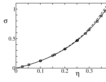
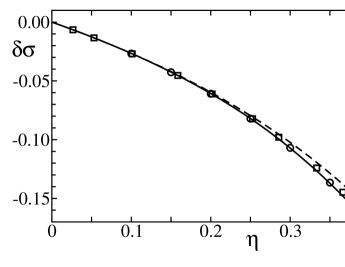
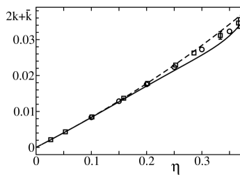
Figure 1: Various curvature coefficients as a function of the fluid volume fraction: (a) surface tension $\sigma$ (in units of $k_{\rm B}T/d^{2}$), (b) Tolman length $\delta\sigma$ (in units of $k_{\rm B}T/d$) and (c) the combination $2k+\bar{k}$ (in units of $k_{\rm B}T$). The drawn lines are the results calculated using Eqs.(33)-(III), transformed according to Eq.(36) so that the radius is defined as that of the “actual surface”. Circular symbols are results from Bryk et al. Bryk03 ; square symbols are the computer simulation results by Laird et al. Laird10 ; Laird12 ; the dashed line is the SPT result in Eq.(III).

Cylindrical interface The analysis for the cylindrical interface is more or less analogous to that of the spherical interface, with one notable difference being that the weight functions $w^{c}_{\alpha}(r_{1},r_{2})$ in Eq.(26) also need to be expanded in $1/R$:

$$w^{c}_{2}(r_{1},r_{2}) = w^{0}_{2}(z_{1}-z_{2})\,\left(1+\frac{d^{2}/4-z_{12}^{2}}{16\,R^{2}}+\ldots\right)\,,$$ (38)

$$w^{c}_{3}(r_{1},r_{2}) = w^{0}_{3}(z_{1}-z_{2})\,\left(1+\frac{d^{2}/4-z_{12}^{2}}{32\,R^{2}}+\ldots\right)\,,$$

$$w^{c}_{3^{\prime}}(r_{1},r_{2}) = w^{0}_{3}(z_{1}-z_{2})\,\left(1+\frac{3(d^{2}/4-z_{12}^{2})}{32\,R^{2}}+\ldots\right)\,,$$

$$w^{c}_{\rm V}(r_{1},r_{2}) = w^{0}_{\rm V}(z_{1}-z_{2})\,\left(1+\frac{d^{2}/4-z_{12}^{2}}{16\,R^{2}}+\ldots\right)\,.$$

Following the same procedure as for the spherical interface, the expressions for $\sigma$ and $\delta\sigma$ in Eqs.(33) and (III) are recovered, and one obtains as an expression for the bending rigidity $k$:

$$\frac{k}{k_{\rm B}T} = -\frac{1}{4}\sum\limits_{\alpha}\int\limits_{-d/2}^{\infty}\!\!\!\!dz_{1}\int\limits_{0}^{\infty}\!\!dz_{2}\;\frac{\partial\phi_{0}}{\partial n^{0}_{\alpha}(z_{1})}\,\rho_{1}(z_{2})\,z_{12}\,w^{0}_{\alpha}(z_{1}-z_{2})$$

$$+\frac{1}{4}\sum\limits_{\alpha,\beta}\int\limits_{-d/2}^{\infty}\!\!\!\!dz_{1}\int\limits_{0}^{\infty}\!\!dz_{2}\;\frac{\partial^{2}\phi_{0}}{\partial n^{0}_{\alpha}(z_{1})\partial n^{0}_{\beta}(z_{1})}\,n^{1}_{\beta}(z_{1})\,\rho_{0}(z_{2})\,z_{12}\,w^{0}_{\alpha}(z_{1}-z_{2})$$

$$+\frac{1}{4}\sum\limits_{\beta}\int\limits_{-d/2}^{\infty}\!\!\!\!dz_{1}\int\limits_{0}^{\infty}\!\!dz_{2}\;\frac{\partial^{2}\phi_{0}}{\partial n^{0}_{\rm V}(z_{1})\partial n^{0}_{\beta}(z_{1})}\,n^{1}_{\beta}(z_{1})\,\rho_{0}(z_{2})\,w^{0}_{3}(z_{1}-z_{2})$$

$$+\frac{1}{8}\sum\limits_{\alpha}\int\limits_{-d/2}^{\infty}\!\!\!\!dz_{1}\int\limits_{0}^{\infty}\!\!dz_{2}\;\frac{\partial\phi_{0}}{\partial n^{0}_{\alpha}(z_{1})}\,\rho_{0}(z_{2})\,(\frac{d^{2}}{4}-3z_{12}^{2})\,w^{0}_{\alpha}(z_{1}-z_{2})$$

$$-\frac{1}{16}\int\limits_{-d/2}^{\infty}\!\!\!\!dz_{1}\int\limits_{0}^{\infty}\!\!dz_{2}\;\frac{\partial\phi_{0}}{\partial n^{0}_{3}(z_{1})}\,\rho_{0}(z_{2})\,(\frac{d^{2}}{4}-z_{12}^{2})\,w^{0}_{3}(z_{1}-z_{2})$$

$$+\frac{1}{4}\int\limits_{-d/2}^{\infty}\!\!\!\!dz_{1}\int\limits_{0}^{\infty}\!\!dz_{2}\;\frac{\partial\phi_{0}}{\partial n^{0}_{\rm V}(z_{1})}\,\rho_{1}(z_{2})\,w^{0}_{3}(z_{1}-z_{2})$$

$$+\frac{1}{2}\int\limits_{-d/2}^{\infty}\!\!\!\!dz_{1}\int\limits_{0}^{\infty}\!\!dz_{2}\;\frac{\partial\phi_{0}}{\partial n^{0}_{\rm V}(z_{1})}\,\rho_{0}(z_{2})\,z_{12}\,w^{0}_{3}(z_{1}-z_{2})\,,$$

where $\rho_{1}(z)$ and $n^{1}_{\alpha}(z)$ are the same as in the spherical analysis. It is noteworthy that since no reference to the location of the $z\!=\!0$ plane is made in this expression, the bending rigidity is independent of the choice for the location of the radius $R$, i.e. $(k)_{\rm R-d/2}\!=\!k$. In this respect the bending rigidity is a much more inherent property of the interface in question. The result of the evaluation of the bending rigidity using Eq.(III) is shown as the solid line in Figure 2. The open circles and crosses are the previous results for $k$ listed in Table 2. Also shown are very recent computer simulation results by Laird et al. Laird12 (solid circles).

Figure 2 is the main result of this article. It shows that the bending rigidity is definitively not equal to zero in the context of FMT theory for a hard sphere fluid near a hard wall and the Hadwiger Theorem does not apply in this case. We have shown this via three more or less independent approaches which agree within numerical accuracy with each other. A further corroboration of this result are the computer simulation results by Laird et al. Laird12 ; although the agreement is not quantitative, the shape of the volume fraction dependence of $k$ is strikingly similar.

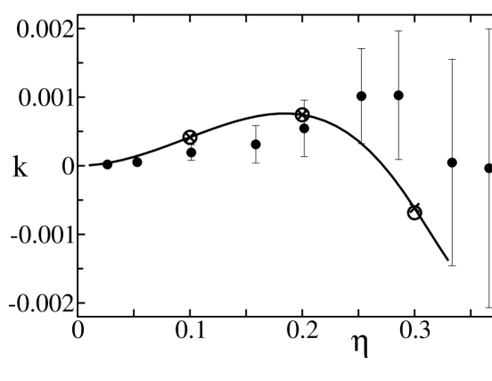
Figure 2: Bending rigidity $k$ (in units of $k_{\rm B}T$) as a function of the fluid volume fraction. The drawn line is the result calculated from Eq.(III); open circles and crosses are the previous results listed in Table 2; solid circles are the computer simulation results by Laird et al. Laird12 .

Finally, we like to mention that by combining the expressions in Eqs.(III) and (III), an expression for the rigidity constant associated with Gaussian curvature may be obtained:

$$\frac{\bar{k}}{k_{\rm B}T} = \int\limits_{-d/2}^{\infty}\!\!\!\!dz\;z^{2}\,\left[\rho_{0}\,\ln(\rho_{0})-\rho_{0}-\frac{\mu}{k_{\rm B}T}\,\rho_{0}+\phi_{0}+\frac{p}{k_{\rm B}T}\,\Theta(z)\right]$$

$$+\sum\limits_{\alpha}\int\limits_{-d/2}^{\infty}\!\!\!\!dz_{1}\int\limits_{0}^{\infty}\!\!dz_{2}\;z_{1}\,\frac{\partial\phi_{0}}{\partial n^{0}_{\alpha}(z_{1})}\,\rho_{0}(z_{2})\,z_{12}\,w^{0}_{\alpha}(z_{1}-z_{2})$$

$$+\int\limits_{-d/2}^{\infty}\!\!\!\!dz_{1}\int\limits_{0}^{\infty}\!\!dz_{2}\;z_{1}\,\frac{\partial\phi_{0}}{\partial n^{0}_{\rm V}(z_{1})}\,\rho_{0}(z_{2})\,w^{0}_{3}(z_{1}-z_{2})$$

$$-\frac{1}{4}\sum\limits_{\alpha}\int\limits_{-d/2}^{\infty}\!\!\!\!dz_{1}\int\limits_{0}^{\infty}\!\!dz_{2}\;\frac{\partial\phi_{0}}{\partial n^{0}_{\alpha}(z_{1})}\,\rho_{0}(z_{2})\,(\frac{d^{2}}{4}-3z_{12}^{2})\,w^{0}_{\alpha}(z_{1}-z_{2})$$

$$+\frac{1}{8}\int\limits_{-d/2}^{\infty}\!\!\!\!dz_{1}\int\limits_{0}^{\infty}\!\!dz_{2}\;\frac{\partial\phi_{0}}{\partial n^{0}_{3}(z_{1})}\,\rho_{0}(z_{2})\,(\frac{d^{2}}{4}-z_{12}^{2})\,w^{0}_{3}(z_{1}-z_{2})\,.$$

Note that $\bar{k}$ can be evaluated from the properties of the planar interface only; a result that is consistent with similar expressions for the liquid-vapour interface Blokhuis93 .

IV Discussion

We have shown that the bending rigidity is not equal to zero in the context of FMT theory for a hard sphere fluid near a hard wall and that the Hadwiger Theorem does not apply in this case. Evidence for this conclusion is shown in Figure 2 where the results of three independent approaches are shown to agree within numerical accuracy. Noteworthy is that the bending rigidity changes sign from positive to negative as a function of increasing fluid volume fraction. It is smaller than the rigidity constant associated with Gaussian rigidity roughly by an order of magnitude.

The reduced magnitude of $k$ may certainly be partly responsible for the fact that in a previous analysis Konig04 it was hard to distinguish it from zero. Another possible source for the discrepancy may be due to a different fit procedure used to extract the curvature coefficients from the radius dependence of the surface tension and wall density. A comparison between our analysis and the analysis in refs. Bryk03 ; Konig04 ; Konig05 shows that while numerical results for $\sigma_{s}(R)$ agree to within a high degree of accuracy Roth_communication , the difference in fit procedure leads to a fitted value for $2k+\bar{k}$ that may differ by as much as 10 % (see Figure 1c). One may very well speculate that the difference in fit procedure used may also have consequences for the fitted value obtained for $k$.

The question now remains, what is the underlying physics of the Hadwiger Theorem? The Hadwiger Theorem is not merely some abstract notion from Mathematics and one should be able to understand more microscopically when the conditions (i.e additivity) that lead to it are fulfilled. To address this question, let us consider the general form of the mean-field expressions for the surface tension in spherical (Eq.(24)) and cylindrical geometry (Eq.(28)) Blokhuis00 :

$$\sigma_{s}(R) = \int\limits\!\!dr\left(\frac{r}{R}\right)^{\!2}\,\Pi_{s}(r)\,,$$ (41)

$$\sigma_{c}(R) = \int\limits\!\!dr\left(\frac{r}{R}\right)\,\Pi_{c}(r)\,,$$

where $\Pi(r)$ depends on the distribution of the fluid density $\rho(r)$ in the interfacial region and may be referred to as the excess free energy density or (the negative of) the excess lateral pressure Blokhuis00 .

Now, if it is assumed that the lateral pressure is independent of $R$, i.e. $\Pi(r)\!=\!\Pi_{0}(z)$, then the only radius dependence in Eq.(41) is due to the geometric factors $(r/R)^{2}$ and $(r/R)$. Therefore, we immediately conclude from Eq.(41) that

$$\sigma = \int\limits\!\!dz\;\Pi_{0}(z)\,,$$ (42)

$$\delta\sigma = -\int\limits\!\!dz\;z\,\Pi_{0}(z)\,,$$

$$\bar{k} = \int\limits\!\!dz\;z^{2}\,\Pi_{0}(z)\,,$$

and the bending rigidity k is zero. Furthermore, all the higher order terms in the expansion in $1/R$ are absent. [It was already Helfrich himself who derived these “geometrical expressions” in terms of progressing moments of the excess lateral pressure HelfLH .] These results correspond precisely to the predictions of the Hadwiger Theorem so that we may conclude that the Hadwiger Theorem corresponds to the statement:

$${\rm Hadwiger\,\,\,Theorem}\hskip 27.0pt\Longleftrightarrow\hskip 27.0pt\Pi(r)=\Pi_{0}(z)\,.$$ (43)

This means that the Hadwiger Theorem applies when the fluid molecules do not rearrange themselves when the curvature of the interface is changed. Certainly, theoretical models may be constructed in which such a rearrangement does not occur, but in general this is certainly not the case. To explore this curvature dependence, we expand $\Pi_{s}(r)$ for a spherical interface in $1/R$:

$$\Pi_{s}(r)=\Pi_{0}(z)+\frac{\Pi_{1}(z)}{R}+\ldots\,.$$ (44)

Szleifer and coworkers Szleifer already showed that the bending rigidity $k$ is then expressed as

$$k=\frac{1}{2}\int\limits\!\!dz\;z\,\Pi_{1}(z)\,,$$ (45)

which explicitly demonstrates the conclusion that $k$ results from the (possible) rearrangement of molecules when the curvature of the interface is changed. An example of such a rearrangement of molecules as described by the density profile $\rho_{1}(z)$ is shown in Figure 3 for $\eta\!=\!$ 0.3.

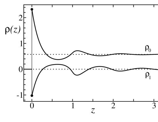
Figure 3: Density profiles $\rho_{0}(z)$ (in units of $1/d^{3}$) and $\rho_{1}(z)$ (in units of $1/d^{2}$) as a function of $z$ (in units of $d$) for $\eta\!=\!$ 0.3. The values at $z\!=\!0$ correspond to the pressure $\rho_{0}(0^{+})\!=\!p/k_{\rm B}T$ and (twice) the surface tension $\rho_{1}(0^{+})\!=\!2\sigma/k_{\rm B}T$; cf. Eq.(8).

Now, one could argue that the vanishing of the bending rigidity is simply a matter of length-scale Konig04 . The length-scale associated with the molecular rearrangement due to curvature is the width of the interfacial region $\xi$, which is small compared any to macroscopic length-scale unless the system is critical RW or when a macroscopic wetting layer is present Evans03 ; Evans04 ; Evans05 . However, the same argument would apply to all the curvature coefficients and in particular to the rigidity constant associated with Gaussian curvature which scales similarly to the bending rigidity.

Acknowledgment This article was inspired by a wonderful presentation by Roland Roth at the Jim Henderson retirement symposium. Further discussions with him and Bob Evans were greatly appreciated. I would also like to thank Brian Laird for communicating his simulation results prior to publication.

References

(1)
W. Helfrich, Z. Naturforsch. C 28, 693 (1973).
(2)
For reviews see Micelles, Membranes, Microemulsions, and Monolayers,
edited by W.M. Gelbart, A. Ben-Shaul, and D. Roux (Springer, New York, 1994);
Statistical Mechanics of Membranes and Surfaces, ed. D. Nelson,
T. Piran, and S. Weinberg (World Scientific, Singapore, 1988).
(3)
S.A. Safran, Statistical Thermodynamics of Surfaces, Interfaces, and Membranes
(Addison-Wesley, Reading, 1994).
(4)
R.C. Tolman, J. Chem. Phys. 17, 333 (1949).
(5)
E.M. Blokhuis and D. Bedeaux, J. Chem. Phys. 97, 3576 (1992).
(6)
E.M. Blokhuis and J. Kuipers, J. Chem. Phys. 124, 074701 (2006).
(7)
P.-M. König, R. Roth, and K.R. Mecke, Phys. Rev. Lett. 93, 160601 (2004).
(8)
P.-M. König, P. Bryk, K.R. Mecke, and R. Roth, Europhys. Lett. 69, 832 (2005).
(9)
H. Hadwiger, Vorlesungen über Inhalt, Oberfläche und Isoperimetrie
(Springer, Berlin, 1957).
(10)
K.R. Mecke, Int. J. Mod. Phys. B 12, 861 (1998).
(11)
P. Bryk, R. Roth, K.R. Mecke, and S. Dietrich, Phys. Rev. E 68, 031602 (2003).
(12)
Y. Rosenfeld, Phys. Rev. Lett. 63, 980 (1989).
(13)
R. Roth, J. Phys. Condens. Matter 22, 063102 (2010).
(14)
J.L. Lebowitz, Phys. Fluids 3, 64 (1960).
(15)
J.R. Henderson, Mol. Phys. 50, 741 (1983).
(16)
J.R. Henderson, in Fluid Interfacial Phenomena,
ed. C.A. Croxton (Wiley, New York, 1986).
(17)
E.M. Blokhuis and J. Kuipers, J. Chem. Phys. 126, 054702 (2007).
(18)
E.M. Blokhuis, unpublished results.
(19)
The absence of this term leads to the striking result in Figure 3 in ref. Konig04 .
It is, however, unrelated to the question whether the bending rigidity vanishes or not.
(20)
E.M. Blokhuis and D. Bedeaux, Mol. Phys. 80, 705 (1993).
(21)
B.B. Laird, A. Hunter, and R.L. Davidchack, Phys. Rev. E 86, 060602 (2012).
(22)
B.B. Laird and R.L. Davidchack, J. Chem. Phys. 132, 204101 (2010).
(23)
R. Roth, R. Evans, A. Lang, and G. Kahl, J. Phys. Condens. Matter 14, 12063 (2002);
Y.-X. Yu and J.Z. Wu, J. Chem. Phys. 117, 10156 (2002).
(24)
N.F. Carnahan and K.E. Starling, Phys. Rev. A 1, 1672 (1970).
(25)
J.S. Rowlinson and B. Widom, Molecular Theory of Capillarity
(Clarendon, Oxford, 1982).
(26)
P.F. Byrd and M.D. Friedman, Handbook of Elliptic Integrals for Engineers and Physicists,
(Springer-Verlag, Berlin, 1954).
(27)
H. Reiss, H.L. Frisch, E. Helfand, and J.L. Lebowitz, J. Chem. Phys. 32, 119 (1960).
(28)
Roland Roth, private communications.
(29)
E.M. Blokhuis, H.N.W. Lekkerkerker, and I. Szleifer, J. Chem. Phys. 112, 6023 (2000).
(30)
W. Helfrich in Physics of Defects, Les Houches, eds. R. Balian et al.
(North-Holland, Amsterdam, 1981).
(31)
I. Szleifer, D. Kramer, A. Ben-Shaul, W.M. Gelbart, and S.A. Safran,
J. Chem. Phys. 92, 6800 (1990); I. Szleifer, D. Kramer, A. Ben-Shaul, D. Roux, and W.M. Gelbart,
Phys. Rev. Lett. 60, 1966 (1988).
(32)
R. Evans, R. Roth, and P. Bryk, Europhys. Lett. 62, 815 (2003).
(33)
R. Evans, J.R. Henderson, and R. Roth, J. Chem. Phys. 121, 12074 (2004).
(34)
M.C. Stewart and R. Evans, Phys. Rev. E 71, 011602 (2005).