Jitter-Adaptive Dictionary Learning - Application to Multi-Trial Neuroelectric Signals

Abstract

Dictionary Learning has proven to be a powerful tool for many image processing tasks, where atoms are typically defined on small image patches. As a drawback, the dictionary only encodes basic structures. In addition, this approach treats patches of different locations in one single set, which means a loss of information when features are well-aligned across signals. This is the case, for instance, in multi-trial magneto- or electroencephalography (M/EEG). Learning the dictionary on the entire signals could make use of the alignment and reveal higher-level features. In this case, however, small misalignments or phase variations of features would not be compensated for. In this paper, we propose an extension to the common dictionary learning framework to overcome these limitations by allowing atoms to adapt their position across signals. The method is validated on simulated and real neuroelectric data.

1 Introduction

The analysis of electromagnetic signals induced by brain activity requires sophisticated tools capable of efficiently treating redundant, multivariate datasets. Redundancy originates for example from the spatial dimension as in multi-channel magneto- or electroencephalography (M/EEG). It can also result from repetitions of the same phenomenon, for instance when a stimulus is presented multiple times to a subject (typically between 50 and 500 times) and the neuronal response is recorded; we will refer to this case as multi-trial analysis.

In the case of multi-channel data, principal component analysis (PCA) [Pearson, 1901] and independent component analysis (ICA) [Comon, 1994] have been successfully used to decompose the data into a few waveforms, providing insight into the underlying neuronal activity and allowing to enhance the often poor signal-to-noise-ratio [Lagerlund et al., 1997, Makeig et al., 1996]. They both use the fact that the data of all channels are recorded synchronically such that features appear well-aligned and phase-locked.

This condition typically does not hold for multi-trial analysis though. In [Woody, 1967] a method is provided to compensate for temporal jitter across signals, but it assumes a single underlying waveform. Matching pursuit (MP) algorithms [Mallat & Zhang, 1993, Durka & Blinowska, 1995] in turn allow to extract several different features and have recently been adapted to deal with multi-channel [Durka et al., 2005, Gribonval, 2003] as well as multi-trial [Bénar et al., 2009] M/EEG data by compensating for different types of variability. However, these methods only allow to extract waveforms that have previously been defined in a dictionary.

In the field of image processing, learning dictionaries directly from the data has shown to yield state-of-the-art results in several applications [Elad & Aharon, 2006, Mairal et al., 2008]. Typically these dictionaries are learned on small patches and represent the basic structures of the images, e.g. edges. When using this technique for neuroelectric multi-trial analysis though, the framework should be carefully adapted to the properties of the data: (i) the waveforms of interest occur approximately at the same time across trials; (ii) however, they may have slightly different time delays (of a small fraction of the signal lenth) or phase variations; (iii) the noise-level is high, partially due to neuronal background activity which is non-Gaussian; (iv) data is often limited to a few hundred signals. The latter two properties make the analysis a difficult problem; it is therefore necessary to incorporate all prior information about the data, in particular (i) and (ii). We note that similar properties can be found in many other signal processing applications, such as in other bioelectric or biomagnetic data (e.g. ECG, EMG).

We suggest that atoms should be learned on the entirety of the signals to provide global high-level features. The common dictionary learning formulation as a matrix factorization problem, however, cannot compensate for the time delays (ii). Existing extensions known as convolutional or shift-invariant sparse coding (SISC) [Smith & Lewicki, 2005, Blumensath & Davies, 2006, Grosse et al., 2007, Ekanadham et al., 2011] learn atoms that are typically smaller than the signal and can occur at arbitrary and possibly multiple positions per signal. This framework is very general for our purpose and does not make use of property (i), the approximate alignment of waveforms. In addition, the SISC framework leads to a highly complex algorithm since all shifts of all atoms are considered in the optimization. The sparse coding step is therefore often handled by heuristic preselection of the active atoms, as described in [Blumensath & Davies, 2006]. But the update of the dictionary elements is also a difficult task, as it involves solving a convolutional problem [Grosse et al., 2007].

In this paper, we present a novel dictionary learning framework that is designed specifically to compensate for small temporal jitter of waveforms across trials, leading to the name jitter-adaptive dictionary learning (JADL). In contrast to SISC, atoms learned by JADL are defined on the entire signal domain and are allowed to shift only up to a small fraction of the signal length. The most important difference, however, is a constraint for atoms to occur at most once (i.e. in one position) per signal, see section 3.2.1. On the one hand, this constraint is reasonable since we do not want to encode a waveform with multiple slightly shifted copies of one atom. On the other hand, it significantly reduces complexity compared to SISC.

An important difference to previous dictionary learning frameworks is the size of the dictionary; while for image processing dictionaries are often overcomplete, JADL aims at learning only a small number of atoms. This is not only desired for easy interpretability, but also because of the difficulties introduced by (iii) and (iv), that make it infeasible to learn a large number of atoms. The “unrolled” version of the dictionary, i.e. the set of all allowed shifts of all atoms may still be large; it therefore makes sense to speak of sparse solutions with respect to this unrolled dictionary. However, JADL enforces sparsity to a major part by the explicit constraint mentioned; sparse regularization only plays a minor role.

We begin by briefly stating the common dictionary learning problem after which we will present the theory and implementation details of JADL. Finally, JADL is evaluated on synthetic and experimental data.

2 Dictionary learning: prior art

A dictionary consists of a matrix ${\mathbf{D}}\in\mathbb{R}^{N\times K}$ that contains for columns the $N$-dimensional column vectors $\{{\mathbf{d}}_{i}\}_{i=1}^{K}$, its atoms. For a set of signals $\{{\mathbf{x}}_{j}\in{\mathbb{R}}^{N}\}_{j=1}^{M}$ the problem of finding a sparse code ${\mathbf{a}}_{j}\in\mathbb{R}^{K}$ for each ${\mathbf{x}}_{j}$ can be formulated as the following minimization problem:

$${\mathbf{a}}_{j}=\operatornamewithlimits{argmin}_{{\mathbf{a}}_{j}\in\mathbb{R}^{K}}\frac{1}{2}\left\|{\mathbf{x}}_{j}-{\mathbf{D}}{\mathbf{a}}_{j}\right\|_{2}^{2}+\lambda\|{\mathbf{a}}_{j}\|_{1}\enspace,$$ (1)

where $\|\cdot\|_{1}$ denotes the $l_{1}$-norm and $\lambda>0$ is a regularization parameter. This problem is known as Lasso [Tibshirani, 1996] and can be solved efficiently with algorithms such as least angle regression (LARS) [Efron et al., 2004] or the proximal methods ISTA [Combettes & Wajs, 2005] and its accelerated version FISTA [Beck & Teboulle, 2009].

The case where ${\mathbf{D}}$ is not known beforehand but shall be estimated given the signals $\{{\mathbf{x}}_{j}\}$, leads to the dictionary learning problem. It is a minimization problem over both the dictionary and the sparse code, which reads:

$$\begin{split}&\min_{{\mathbf{D}},{\mathbf{a}}_{j}}\frac{1}{2}\sum_{j=1}^{M}\left(\left\|{\mathbf{x}}_{j}-{\mathbf{D}}{\mathbf{a}}_{j}\right\|_{2}^{2}+\lambda\left\|{\mathbf{a}}_{j}\right\|_{1}\right),\\ &\text{s.t.}\quad\|{\mathbf{d}}_{i}\|_{2}=1,\quad i=1,\ldots,K,\end{split}$$ (2)

where the latter constraint prevents atoms from growing arbitrarily large.

Most algorithms tackle this non-convex problem iteratively by alternating between the convex subproblems: (i) the sparse coding (with ${\mathbf{D}}$ fixed) and (ii) the dictionary update ($\{{\mathbf{a}}_{j}\}_{j=1}^{M}$ fixed). The first such algorithm was provided in the pioneer work on dictionary learning in [Olshausen & Field, 1997]. Many alternatives have been proposed, such as the method of optimal directions (MOD) in [Engan et al., 1999], $K$-SVD [Aharon et al., 2006], or more recently an online version [Mairal et al., 2010] to handle large datasets.

3 Jitter-adaptive dictionary learning

This section introduces the main contribution of this paper: a novel technique designed to overcome the limitations of purely linear signal decomposition methods such as PCA, ICA, and dictionary learning.

We suppose that atoms present in a signal can suffer from unknown time delays, which we will refer to as jitter. This type of variability addresses the issue of varying latencies of transient features as well as oscillations with different phases across trials.

This issue is very important for interpretation of M/EEG data, to answer fundamental questions such as the link between evoked responses and oscillatory activity [Hanslmayer et al., 2007, Mazaheri & Jensen, 2008], the correlation between single-trial activity and behavioral data [Jung et al., 2001], the variability of evoked potentials such as the P300 [Holm et al., 2006]. Cross-trial variability is also a precious source of information for simultaneous EEG-fMRI interpretation [Bénar et al., 2007].

We therefore provide a dictionary learning framework in which atoms may adapt their position across trials. This framework can be generalized to address other kinds of variability; the shift operator introduced below can simply be replaced by the desired operators. The entire framework remains the same, only the formula for the update of the dictionary needs to be adapted as described in Section 3.2.2.

3.1 Model and problem statement

Our model is based on the hypothesis that the set of signals of interest $\{{\mathbf{x}}_{j}\}_{j=1}^{M}$ can be generated by a dictionary ${\mathbf{D}}=\{{\mathbf{d}}_{i}\}_{i=1}^{K}$ with few atoms $K$ in the following way: Given a set of shift operations $\Delta$ , for every $j$ there exist coefficients $a_{ij}\in{\mathbb{R}}$ and shift operators $\delta_{ij}\in\Delta$, such that

$${\mathbf{x}}_{j}=\sum_{i=1}^{K}a_{ij}\delta_{ij}({\mathbf{d}}_{i})\enspace.$$ (3)

We assume that $\Delta$ contains only small shifts relative to the size of the time window. Now, we can formulate the jitter-adaptive dictionary learning problem

$$\begin{split}&\min_{{\mathbf{d}}_{i},a_{ij},\delta_{ij}}\sum_{j=1}^{M}\left(\frac{1}{2}\left\|{\mathbf{x}}_{j}-\sum_{i=1}^{K}a_{ij}\delta_{ij}({\mathbf{d}}_{i})\right\|_{2}^{2}+\lambda\left\|{\mathbf{a}}_{j}\right\|_{1}\right),\\ &\text{s.t.}\quad\left\|{\mathbf{d}}_{i}\right\|_{2}=1,\quad\delta_{ij}\in\Delta,\quad i=1,\ldots,K,\quad j=1,\ldots,M.\end{split}$$ (4)

Note that for $\Delta=\{{\mathbf{I}}\}$ this reduces to Eq. (2), the problem is thus also non-convex and we solve it similarly using alternate minimizations.

3.2 Implementation

The algorithm that we propose for solving Eq. (4) is based on an implementation in [Mairal et al., 2010] for common dictionary learning, which iteratively alternates between (i) sparse coding and (ii) dictionary update. We adapt the algorithm least angle regression (LARS) used for solving (i) to find not only the coefficients $\{a_{ij}\}$ but also the latencies $\{\delta_{ij}\}$. For (ii), block coordinate descent is used. The entire procedure is summarized in Algorithm 1 (notation and details are explained in the following).

Algorithm 1 Jitter-Adaptive Dictionary Learning

0:  $\text{signals }\{{\mathbf{x}}_{1},{\mathbf{x}}_{2},\ldots,{\mathbf{x}}_{M}\},\text{shift operators }\Delta,K\in\mathbb{N},\lambda\in\mathbb{R},$

1:  Initialize ${\mathbf{D}}=\{{\mathbf{d}}_{1},{\mathbf{d}}_{2},\ldots,{\mathbf{d}}_{K}\}$

2:  repeat

3:     Set up “unrolled” dictionary ${\mathbf{D}}^{S}$ from ${\mathbf{D}}$

4:     Sparse coding (solve using modified LARS)

5:     for $j=1$ to $M$ do

6:        

$${\mathbf{a}}^{S}_{j}\leftarrow\operatornamewithlimits{argmin}\frac{1}{2}\left\|{\mathbf{x}}_{j}-{\mathbf{D}}^{S}{\mathbf{a}}^{S}_{j}\right\|_{2}^{2}+\lambda\left\|{\mathbf{a}}^{S}_{j}\right\|_{1},\quad\text{s.t.}\quad\left\|{\mathbf{a}}_{j}^{S,i}\right\|_{0}\leq 1$$

7:     end for

8:     Convert $\{{\mathbf{a}}^{S}_{j}\}$ to $\{a_{ij}\},\{\delta_{ij}\}$

9:     Dictionary update (solve using block coordinate descent)

10:     

$${\mathbf{D}}\leftarrow\operatornamewithlimits{argmin}_{\{{\mathbf{d}}_{i}\}_{i=1}^{K}}\sum_{j=1}^{M}\frac{1}{2}\left\|{\mathbf{x}}_{j}-\sum_{i=1}^{K}a_{ij}\delta_{ij}({\mathbf{d}}_{i})\right\|_{2}^{2},\quad\text{s.t.}\quad\|{\mathbf{d}}_{i}\|=1$$

11:  until convergence

3.2.1 Sparse coding

When ${\mathbf{D}}$ is fixed, the minimization Eq. (4) can be solved independently for each signal ${\mathbf{x}}_{j}$,

$$\min_{a_{ij},\delta_{ij}}\frac{1}{2}\left\|{\mathbf{x}}_{j}-\sum_{i=1}^{K}a_{ij}\delta_{ij}({\mathbf{d}}_{i})\right\|_{2}^{2}+\lambda\left\|{\mathbf{a}}_{j}\right\|_{1}.\\$$ (5)

We now rewrite this problem into a form similar to the Lasso, which allows us to solve it using a modification of LARS. Let us first define an “unrolled” version of the dictionary containing all possible shifts of all its atoms; this is given by ${\mathbf{D}}^{S}=\{\delta({\mathbf{d}}):{\mathbf{d}}\in{\mathbf{D}},\delta\in\Delta\}$, a matrix of dimension ${N\times KS}$, where $S=|\Delta|$ is the number of allowed shifts. The decomposition in Eq. (5) can now be rewritten as a linear combination over the unrolled dictionary

$$\sum_{i=1}^{K}a_{ij}\delta_{ij}({\mathbf{d}}_{i})={\mathbf{D}}^{S}{\mathbf{a}}^{S}_{j},$$

where ${\mathbf{a}}^{S}_{j}\in{\mathbb{R}}^{KS}$ denotes the corresponding coefficient vector. This vector is extremely sparse; in fact, each subvector ${\mathbf{a}}^{S,i}_{j}$ of ${\mathbf{a}}^{S}_{j}$ that contains the coefficients corresponding to the shifts of atom ${\mathbf{d}}_{i}$ shall maximally have one non-zero entry. If such a non-zero entry exists, its position indicates which shift was used for atom ${\mathbf{d}}_{i}$. Now Eq. (5) can be rewritten as

$${\mathbf{a}}^{S}_{j}\leftarrow \operatornamewithlimits{argmin} \frac{1}{2}\left\|{\mathbf{x}}_{j}-{\mathbf{D}}^{S}{\mathbf{a}}^{S}_{j}\right\|_{2}^{2}+\lambda\left\|{\mathbf{a}}^{S}_{j}\right\|_{1},$$ (6)

s.t. $$\quad\left\|{\mathbf{a}}_{j}^{S,i}\right\|_{0}\leq 1,\quad i=1,\ldots,K.$$ (7)

Clearly, Eq. (6) is the Lasso, but the constraint (7) leads to a non-convex problem. Therefore the modification of the LARS that we propose below only guarantees convergence to a local minimum.

The LARS algorithm [Efron et al., 2004] follows a stepwise procedure; in each step the coefficient of one atom is selected to change from “inactive” to “active” (i.e. it changes from zero to non-zero) or vice versa. In order to enforce the constraint (7), we make the following modification. When a coefficient is selected for activation, we determine the index $i$ such that this coefficient lies in ${\mathbf{a}}_{j}^{S,i}$. We then block all other coefficients contained in the subvector ${\mathbf{a}}_{j}^{S,i}$ such that they cannot get activated in a later step. In the same manner, we unblock all entries of ${\mathbf{a}}_{j}^{S,i}$ when its active coefficient is deactivated.

As mentioned in the introduction, the constraint (7), which is the main difference to SISC, helps to reduce the complexity of the optimization. In fact, each time an atom is activated, all its translates are blocked and do not need to be considered in the following steps, which facilitates the calculation. In addition, maximally $K$ steps have to be performed (given that no atom is deactivated in a later step, which we observed to occur rarely). As suggested for example in [Grosse et al., 2007] the inital correlations of the shifted atoms with the signal can be computed using fast convolution via FFT, which speeds up computation in the case of a large number of shifts $S$.

3.2.2 Dictionary update

For the dictionary update, its unrolled version cannot be used as this would result in updating different shifts of the same atom in different ways. Instead, the shifts have to be explicitly included in the update process. We use block coordinate descent to iteratively solve the constrained minimization problem

$${\mathbf{d}}_{k}=\operatornamewithlimits{argmin}_{{\mathbf{d}}_{k}}\sum_{j=1}^{M}\frac{1}{2}\left\|{\mathbf{x}}_{j}-\sum_{i=1}^{K}a_{ij}\delta_{ij}({\mathbf{d}}_{i})\right\|_{2}^{2},\quad\text{s.t.}\quad\|{\mathbf{d}}_{k}\|_{2}=1$$

for each atom ${\mathbf{d}}_{k}$. This can be solved in two steps, the solution of the unconstrained problem by differentiation followed by normalization. This is summarized by

$$\widetilde{{\mathbf{d}}_{k}} = \sum_{j=1}^{M}a_{kj}\delta_{kj}^{-1}\left({\mathbf{x}}_{j}-\sum_{i\neq k}a_{ij}\delta_{ij}({\mathbf{d}}_{i})\right),$$ (8)

$${\mathbf{d}}_{k} = \frac{\widetilde{{\mathbf{d}}_{k}}}{\|\widetilde{{\mathbf{d}}_{k}}\|_{2}}.$$

with $\delta^{-1}$ the opposite shift of $\delta$. As in [Mairal et al., 2010], we found that one update loop through all of the atoms was enough to ensure fast convergence of Algorithm 1.

The only difference of this update compared to common dictionary learning are the shift operators $\delta_{ij}$. In contrast to the sparse coding step, the jitter adaptivity therefore does not increase the complexity for this step. When high efficiency of the algorithm is needed, this fact can be used by employing mini-batch or online techniques [Mairal et al., 2010], which increase the frequency of dictionary update steps with respect to sparse coding steps.

We note that in Eq. (8) we assumed the shifts to be circular; being orthogonal transforms, i.e. $\delta\delta^{t}={\mathbf{I}}$, they provide for a simple update formula. In the case of non-circular shifts or other linear operators, the inverse $\delta_{kj}^{-1}$ in the update Eq. (8) needs to be replaced by the adjoint $\delta_{kj}^{t}$. In addition, the rescaling function $\psi=(\sum_{j=1}^{M}a_{kj}^{2}\delta_{kj}\delta^{t}_{kj})^{-1}$ has to be applied to the update term.

3.2.3 Hyperparameters and initial dictionary

As mentioned before, the optimal number $K$ of atoms will typically be lower than for dictionary learning in image processing frameworks; this is due to the high redundancy of the electromagnetic brain signals as well as the adaptive property of the atoms. When oscillatory activity is sought, $\Delta$ should contain shifts of up to the largest period expected to be found. The choice of $\lambda$ plays a less important role than in common dictionary learning; most of the sparsity is induced directly by the constraint (7).

The choice of the initial dictionary can be crucial for the outcome, due to the non-convex nature of the problem. Especially when the initial dictionary already produces a small sparse coding error, the algorithm may converge to a local minimum that is very close to the initialization. While this property allows us to incorporate a priori knowledge by initializing with a predefined dictionary, this also provides the risk of preventing the algorithm from learning interesting features if they are “far” from the initial dictionary.

Figure 1: Original dictionary and reconstructions with PCA, DL, and JADL, respectively; row 5: similarity $\rho$ and average energy across signals $\bar{E}$ for each atom, the dashed line marks the value 1 in both plots.

Figure 2: Clean, noisy and denoised signals, row 1: clean signals; row 2: signals plus spurious events; row 3: signals above plus white noise, row 4-6: denoised signals using PCA, DL, and JADL, respectively.

When no dictionary is given a priori, initializations often found in the literature include random values as in [Olshausen & Field, 1997] as well as random examples [Aharon et al., 2006] or linear combinations (e.g. PCA) of the input signals. In order to keep the bias towards the initialization as small as possible, we favor random initializations independent from the signals.

4 Experiments

Jitter-adaptive dictionary learning (JADL) is next evaluated on synthetic and on experimental data. Its performance is compared to results obtained with principal component analysis (PCA)[Pearson, 1901] and dictionary learning (DL); for the latter we used the open-source software package SPAMS whose implementation is described in [Mairal et al., 2010].

4.1 Synthetic data

Table 1: First three rows: average similarity $\bar{\rho}$ of original and reconstructed atoms; last two rows: parameter $\lambda$ used for reconstruction.

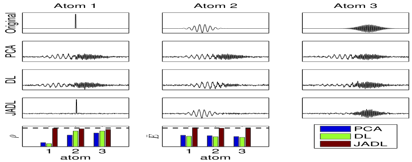
Generating the dictionary: First, a dictionary ${\mathbf{D}}$ with $K=3$ normalized atoms was defined, as shown in Figure 2 (first row). The first atom is a delta-shaped spike and the other two are oscillatory features. The length of the time window was chosen as $4$ seconds and the sampling rate as 128 Hz, hence $N=512$.

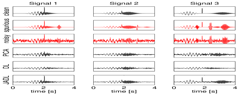
Generating the signals: From the dictionary, $M=200$ signals were generated according to the model Eq. (3). The coefficients ${\mathbf{a}}_{ij}$ and shifts $\delta_{ij}$ were drawn independently from Gaussian distributions with mean $\mu=1$ and standard deviation $\sigma=0.3$ for the coefficients and $\mu=0,\sigma=0.2$ s for the shifts. Three examples are shown in the first row of Figure 2. These signals were then corrupted by two types of noise: (i) to every signal between $0$ and $3$ oscillatory events were added, their amplitudes, frequencies, temporal supports and positions in time were drawn randomly (Fig. 2, row 2); (ii) then white Gaussian noise with a resulting average SNR (energy of clean signals/energy of noise) of 0.790 was added (row 3).

Reconstructions: Performance of the three methods PCA, DL, and JADL given the noisy signals (Fig. 2, row 3) was measured on both their ability of recovering the original dictionary and the denoising of the signals. We performed reconstruction for different dictionary sizes $K$. For DL and JADL we chose the $\lambda$ that gave the best results; we noticed relatively small sensitivity of the methods to the choice of $\lambda$, especially for small values of $K$.

Recovering the dictionary: For PCA, the dictionary atoms were defined as the first $K$ principal components. For JADL, the set $\Delta$ was defined to contain all time shifts of maximally $\pm 0.6$ seconds, resulting in $S=128\text{ Hz}\cdot 1.2\text{ s}\approx 154$ allowed shifts. For each reconstructed dictionary, the three atoms that showed the highest similarity $\rho$ to the original atoms were used to calculate the average similarity $\bar{\rho}$. $\rho$ was defined as the maximal correlation of the reconstructed atom and all shifts of maximally $\pm 0.6$ seconds of the original atom. The values $\bar{\rho}$ are shown for PCA, DL, and JADL in Table 1 for each $K$ (for $K>12$ we observed decreasing similarity values for all three methods). The similarity for JADL is significantly higher than for PCA and DL; its optimal value is obtained for $K=3$ atoms, but it remains high for larger $K$, showing its robustness to overestimation of original atoms. Note that dictionaries obtained by PCA for different values of $K$ always have their first atoms in common, hence the constant similarity values.

Table 2: Relative $l_{2}$-error $\epsilon$ produced by each method for different $K$; the last two rows show the values of $\lambda$ used for DL and JADL.

For each method, the $K$ giving the highest similarity was determined and the three atoms with largest $\rho$-values of the corresponding dictionaries are shown in Figure 2 (row $2$ - $4$). The atoms found by PCA and DL contain only mixtures of the oscillatory atoms, the spike does not appear at all. JADL succeeds in separating the three atoms; their shapes and average energy across signals $\bar{E}$ are very close to the originals, as shown in the bar plots.

Denoising the signals: For PCA, denoising was performed by setting the coefficients of all but the first $K$ components to zero. For DL and JADL, the noisy signals were encoded over the learned dictionaries according to Eq. (1) and (5), respectively. Table 2 shows the average relative $l_{2}$-errors $\epsilon$ of all denoised signals with respect to the original ones. For each method, three denoised signals for optimal $K$ are shown in the last three rows of Figure 2. Despite the larger dictionary size ($K=8$) in the case of PCA and DL, the spike could not be reconstructed due to its jitter across signals. In addition, the locations of the oscillatory events in the signals denoised with JADL correspond better to their true locations than it is the case for PCA and DL, especially in the last signal shown. Finally, the white noise appears more reduced for JADL, which is due to its smaller dictionary size. All three methods succeeded in removing the spurious events from the signals.

4.2 Real data

Local field potentials (LFP) were recorded with an intra-cranial electrode in a Wistar-Han rat, in an animal model of epilepsy. Bicuculline (a blocker of inhibition) was injected in the cortex in order to elicit epileptic-like discharges. Discharges were selected visually on the LFP traces, and the data was segmented in 169 epochs centered around the spikes. To simplify the analysis, the epochs were scaled with a constant factor such that the maximal $l_{2}$-energy among epochs was equal to $1$.

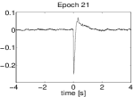
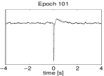
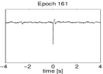
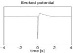
Three examples of epochs are shown in Figure 3, as well as the evoked potential, measured as the average over the epochs. The only structure visible to the eye is a spike with changing shape and decreasing energy across epochs.

Figure 3: Different epochs of the local field potential (LFP) showing spikes with decreasing energy; the evoked potential (last) is the average over all epochs.

Figure 4: Dictionaries learned on LFP epochs using PCA, DL, and JADL.

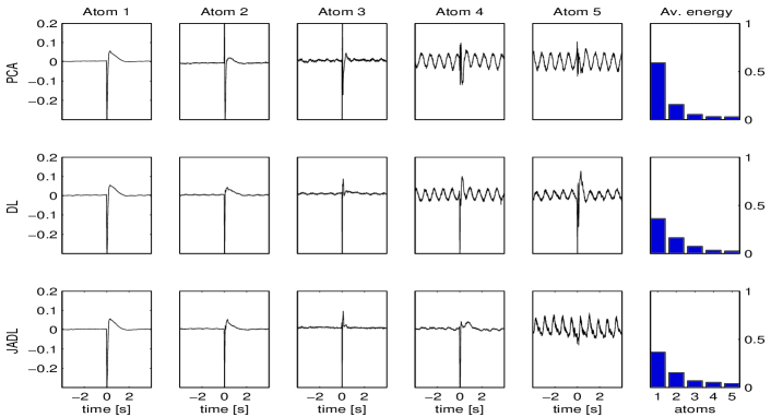
Learning the dictionary: Five normalized atoms were learned on the data with PCA, DL and JADL; see Figure 4. They were ordered in descending order of their average energy across epochs.

All three methods produce for their first atom a spike that resembles the evoked potential (Figure 3); also, all methods reveal an oscillatory artifact around 1.2 Hz which is not visible in the evoked potential. However, while the oscillations in the PCA and DL dictionaries are encoded in two atoms (4 and 5) that differ mostly in phase, they are concentrated in atom 5 for JADL. Additionally, in the case of JADL the oscillations are almost completely separated from the spike, only a small remainder is still visible. This shows the need of PCA and DL for several atoms to compensate for phase shifts while JADL is able to associate oscillations with different phases; moreover JADL makes use of the varying phases to clearly separate transient from oscillatory events. In addition, we can observe a smoothing effect in the case of PCA and DL: the oscillations look very much like sinusoids whereas atom 5 in JADL shows a less smooth, rather spiky structure.

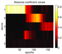
Interpreting the code: We visualized the coefficients and the shifts obtained by decomposing all the epochs over the dictionary learned with JADL, see Figure 5. Interestingly, each of the first three spikes in the dictionary is active during a contiguous set of epochs during which the other atoms are hardly used. This allows to segment the epochs into three sets of different spike shapes. The fourth atom is only active during a few epochs where the dominant atom is changing from the first to the second spike. The oscillatory artifact (atom 5) in contrast shows very low but constant activity across all epochs.

The latency distributions (Fig. 5(b)) can provide further insight into the data. The highly peaked distribution for the first atoms gives evidence of the accurate alignment of the spikes. The last atom shows shifts in the whole range from $-0.4$ to $0.4$ seconds, indicating that the phases of the oscillations were uniformly distributed across epochs.

Computation times: The dictionary and the code above were obtained for 189 iterations of JADL after which the algorithm converged. The time of computation on a laptop (Intel Core CPU, 2.4 GHz) was 4.3 seconds. As JADL is designed for datasets of similar complexity to the one investigated here, computation time should not be an issue for offline analysis. However, applications such as M/EEG based brain computer interfaces (BCI) may require computations in real time. We remark that our implementation has not yet been optimized and could be speeded up significantly by parallelization or online techniques mentioned in section 3.2.2. If training data is available beforehand, the dictionary may also be calculated offline in advance; the sparse encoding of new data over this dictionary then only takes up a small fraction of the training time and can be performed online.

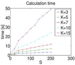
Figure 5(c) illustrates the effect of changing the number of atoms $K$ and shifts $S$ on computation time $t$; for each calculation 200 iterations were performed. We can see that $t$ is linearly correlated with $S$ but increases over-linearly with $K$: while both, $S$ and $K$ affect the size of the unrolled dictionary ${\mathbf{D}}^{S}$, an increase of $S$ is handled more efficiently by using calculation advantages described in section 3.2.1; e.g., the non-smooth behavior of the curves at $S=40$ results from the fact that for $S>40$ an FFT-based convolution is used. In addition, the dictionary update step only uses the compact dictionary ${\mathbf{D}}$ whose size does not increase with $S$. If the additional factor in computation time due to $S$ is still not acceptable, $\Delta$ may be subsampled by introducing a minimal distance between shifts; the tradeoff is a less exact description of the atoms latencies.

(a) Absolute coefficients of atoms learned with JADL.

(b) Distribution of latencies for each atom.

(c) Computation times for different values of $S$ and $K$.

Figure 5: Code visualization and computation times.

5 Conclusion

In this paper, a novel method for the analysis and processing of multi-trial neuroelectric signals was introduced. The method was derived by extending the dictionary learning framework, allowing atoms to adapt to jitter across trials; hence the name jitter-adaptive dictionary learning (JADL). It was shown how the resulting non-convex minimization problem can be tackled by modifying existing algorithms used in common dictionary learning.

The method was validated on synthetic and experimental data, both containing variability in latencies of transient and in the phases of oscillatory events. The results obtained showed to be superior to those of common dictionary learning and PCA, both in recovering the underlying dictionary and in denoising the signals. The evaluation furthermore demonstrated the usefulness of JADL as a data exploration tool, capable of extracting global, high-level features of the signals and giving insight into their distributions.

Acknowledgments

This work was supported by the doctoral grant of the region Provence-Alpes-Côte d’Azur and the ANR grants CoAdapt (09-EMER-002-01) and MultiModel (2010 BLAN 0309 04).

References

- Aharon et al., 2006 Aharon, M., Elad, M., & Bruckstein, A. 2006. K-SVD: An Algorithm for Designing Overcomplete Dictionaries for Sparse Representation. IEEE Transactions on Signal Processing, 54(11), 4311–4322.
- Beck & Teboulle, 2009 Beck, A., & Teboulle, M. 2009. A fast iterative shrinkage-thresholding algorithm for linear inverse problems. SIAM Journal on Imaging Sciences, 2(1), 183–202.
- Bénar et al., 2007 Bénar, C.G., Schön, D., Grimault, S., Nazarian, B., Burle, B., Roth, M., Badier, J.M., Marquis, P., Liegeois-Chauvel, C., & Anton, J.L. 2007. Single-trial analysis of oddball event-related potentials in simultaneous EEG-fMRI. Human Brain Mapping, 28, 602–613.
- Bénar et al., 2009 Bénar, C.G., Papadopoulo, T., Torrésani, B., & Clerc, M. 2009. Consensus matching pursuit for multi-trial EEG signals. Journal of neuroscience methods, 180(1), 161–170.
- Blumensath & Davies, 2006 Blumensath, Thomas, & Davies, Mike. 2006. Sparse and shift-invariant representations of music. Audio, Speech, and Language Processing, IEEE Transactions on, 14(1), 50–57.
- Combettes & Wajs, 2005 Combettes, P. L., & Wajs, V. R. 2005. Signal recovery by proximal forward-backward splitting. Multiscale Modeling and Simulation, 4(4), 1168–1200.
- Comon, 1994 Comon, P. 1994. Independent component analysis, a new concept? Signal processing, 36(3), 287–314.
- Durka & Blinowska, 1995 Durka, PJ, & Blinowska, KJ. 1995. Analysis of EEG transients by means of matching pursuit. Annals of biomedical engineering, 23(5), 608–611.
- Durka et al., 2005 Durka, P.J., Matysiak, A., Montes, E.M., Sosa, P.V., & Blinowska, K.J. 2005. Multichannel matching pursuit and EEG inverse solutions. Journal of neuroscience methods, 148(1), 49–59.
- Efron et al., 2004 Efron, B., Hastie, T., Johnstone, I., & Tibshirani, R. 2004. Least angle regression. The Annals of statistics, 32(2), 407–499.
- Ekanadham et al., 2011 Ekanadham, Chaitanya, Tranchina, Daniel, & Simoncelli, Eero P. 2011. Sparse decomposition of transformation-invariant signals with continuous basis pursuit. Pages 4060–4063 of: Acoustics, Speech and Signal Processing (ICASSP), 2011 IEEE International Conference on. IEEE.
- Elad & Aharon, 2006 Elad, M., & Aharon, M. 2006. Image denoising via sparse and redundant representations over learned dictionaries. Image Processing, IEEE Transactions on, 15(12), 3736–3745.
- Engan et al., 1999 Engan, K., Aase, S.O., & Hakon Husoy, J. 1999. Method of optimal directions for frame design. Pages 2443–2446 of: Acoustics, Speech, and Signal Processing, 1999. Proceedings., 1999 IEEE International Conference on, vol. 5. IEEE.
- Gribonval, 2003 Gribonval, R. 2003. Piecewise linear source separation. Pages 297–310 of: Optical Science and Technology, SPIE’s 48th Annual Meeting. International Society for Optics and Photonics.
- Grosse et al., 2007 Grosse, R, Raina, R, Kwong, H, & Ng, AY. 2007. Shift-invariant sparse coding for audio classification. In: Proceedings of the Twenty-third Conference on Uncertainty in Artificial Intelligence (UAI’07).
- Hanslmayer et al., 2007 Hanslmayer, S., Klimesch, W., Sauseng, P., Gruber, W., Dopplemayr, M., Freunberger, R., Pecherstorfer, T., & Birbaumer, N. 2007. Alpha phase reset contributes to the generation of ERPs. Cerebral Cortex, 17, 1–8.
- Holm et al., 2006 Holm, A., Ranta-aho, P., Sallinen, M., Karjalainen, P., & Müller, K. 2006. Relationship of P300 single-trial responses with reaction time and preceding stimulus sequence. Int. J. Psychophysiol.
- Jung et al., 2001 Jung, T.P., Makeig, S., Westerfield, M., Townsend, J., Courchesne, E., & Sejnowski, T.J. 2001. Analysis and Visualization of Single-Trial Event-Related Potentials. Human Brain Mapping, 14, 166–185.
- Lagerlund et al., 1997 Lagerlund, T.D., Sharbrough, F.W., & Busacker, N.E. 1997. Spatial filtering of multichannel electroencephalographic recordings through principal component analysis by singular value decomposition. Journal of Clinical Neurophysiology, 14(1), 73–82.
- Mairal et al., 2008 Mairal, J., Bach, F., Ponce, J., Sapiro, G., & Zisserman, A. 2008. Supervised dictionary learning. arXiv preprint arXiv:0809.3083.
- Mairal et al., 2010 Mairal, J., Bach, F., Ponce, J., & Sapiro, G. 2010. Online Learning for Matrix Factorization and Sparse Coding. Journal of Machine Learning Research, 11(Aug.), 19–60.
- Makeig et al., 1996 Makeig, S., Bell, A.J., Jung, T.P., Sejnowski, T.J., et al. 1996. Independent component analysis of electroencephalographic data. Advances in neural information processing systems, 145–151.
- Mallat & Zhang, 1993 Mallat, S.G., & Zhang, Z. 1993. Matching pursuits with time-frequency dictionaries. Signal Processing, IEEE Transactions on, 41(12), 3397–3415.
- Mazaheri & Jensen, 2008 Mazaheri, A., & Jensen, O. 2008. Amplitude modulations of brain oscillations generate slow evoked responses. Journal of Neuroscience, 28, 7781–7787.
- Olshausen & Field, 1997 Olshausen, B.A., & Field, D.J. 1997. Sparse coding with an overcomplete basis set: a strategy employed by V1? Vision research, 37(23), 3311–25.
- Pearson, 1901 Pearson, K. 1901. LIII. On lines and planes of closest fit to systems of points in space. The London, Edinburgh, and Dublin Philosophical Magazine and Journal of Science, 2(11), 559–572.
- Smith & Lewicki, 2005 Smith, Evan, & Lewicki, Michael S. 2005. Efficient coding of time-relative structure using spikes. Neural Computation, 17(1), 19–45.
- Tibshirani, 1996 Tibshirani, R. 1996. Regression shrinkage and selection via the lasso. Journal of the Royal Statistical Society. Series B (Methodological), 267–288.
- Woody, 1967 Woody, C.D. 1967. Characterization of an adaptive filter for the analysis of variable latency neuroelectric signals. Medical and Biological Engineering and Computing, 5(6), 539–554.