Model Selection for Gaussian Mixture Models

Abstract

This paper is concerned with an important issue in finite mixture modelling, the selection of the number of mixing components. We propose a new penalized likelihood method for model selection of finite multivariate Gaussian mixture models. The proposed method is shown to be statistically consistent in determining of the number of components. A modified EM algorithm is developed to simultaneously select the number of components and to estimate the mixing weights, i.e. the mixing probabilities, and unknown parameters of Gaussian distributions. Simulations and a real data analysis are presented to illustrate the performance of the proposed method.

Key Words: Gaussian mixture models, Model selection, Penalized likelihood, EM algorithm.

1 Introduction

Finite mixture modeling is a flexible and powerful approach to modeling data that is heterogeneous and stems from multiple populations, such as data from patter recognition, computer vision, image analysis, and machine learning. The Gaussian mixture model is an important mixture model family. It is well known that any continuous distribution can be approximated arbitrarily well by a finite mixture of normal densities (Lindsay, 1995; McLachlan and Peel, 2000). However, as demonstrated by Chen (1995), when the number of components is unknown, the optimal convergence rate of the estimate of a finite mixture model is slower than the optimal convergence rate when the number is known. In practice, with too many components, the mixture may overfit the data and yield poor interpretations, while with too few components, the mixture may not be flexible enough to approximate the true underlying data structure. Hence, an important issue in finite mixture modeling is the selection of the number of components, which is not only of theoretical interest, but also significantly useful in practical applications.

Most conventional methods for determining the order of the finite mixture model are based on the likelihood function and some information theoretic criteria, such as AIC and BIC. Leroux (1992) investigated the properties of AIC and BIC for selecting the number of components for finite mixture models and showed that these criteria would not underestimate the true number of components. Roeder and Wasserman (1997) showed the consistency of BIC when a normal mixture model is used to estimate a density function “nonparametrically”. Using the locally conic parameterization method developed by Dacunha-Castelle and Gassiat (1997), Keribin (2000) investigated the consistency of the maximum penalized likelihood estimator for an appropriate penalization sequence. Another class of methods is based on the distance measured between the fitted model and the nonparametric estimate of the population distribution, such as penalized minimum-distance method (Chen and Kalbfleisch, 1996), the Kullback-Leibler distance method (James, Priebe and Marchette, 2001) and the Hellinger distance method (Woo and Sriram, 2006). To avoid the irregularity of the likelihood function for the finite mixture model that emerges when the number of components is unknown, Ray and Lindsay (2008) suggested to use a quadratic-risk based approach to select the number of components for the finite multivariate mixture. However, these methods are all based on the complete model search algorithm and the computation burden is heavy. To improve the computational efficiency, recently, Chen and Khalili (2008) proposed a penalized likelihood method with the SCAD penalty (Fan and Li, 2001) for mixtures of univariate location distributions. They proposed to use the SCAD penalty function to penalize the differences of location parameters, which is able to merge some subpopulations by shrinking such differences to zero. However, similar to most conventional order selection methods, their penalized likelihood method can be only used for one dimensional location mixture models. Furthermore, if some components in the true/optimal model have the same location (which is the case for the experiment in Subsection 4.2 of this study), some of them would be eliminated incorrectly by this method.

On the other hand, Bayesian approaches have been also used to find a suitable number of components of the finite mixture model. For instance, variational inference, as an approximation scheme of Bayesian inference, can be used to determine the number of the components in a fully Bayesian way (see, e.g., Corduneanu and C.M. Bishop (2001) or Chapter 10.2 of Bishop (2006)). Moreover, with suitable priors on the parameters, the maximum a posteriori (MAP) estimator can be used for model selection. In particular, Ormoneit and Tresp (1998) and Zivkovic and van der Heijden (2004) put the Dirichlet prior on the mixing weights, i.e. the mixing probabilities, of the components in the Gaussian mixture model, and Brand (1999) applied the “entropic prior” on the same parameters to favor models with small entropy. They then used the MAP estimator to drive the mixing weights associated with unnecessary components toward extinction. Based on an improper Dirichlet prior, Figueiredo and Jain (2002) suggested to use minimum message length criterion to determine the number of the components, and further proposed an efficient algorithm for learning a finite mixture from multivariate data. We would like to point out the significant difference between those approaches and our proposed method in this paper. When a component is eliminated, our suggested objective function changes continuously, while those approaches encounter a sudden change in the objective function because $zero$ is not in the support area of the prior distribution for the mixing weights, such as the Dirichlet prior. Therefore, it is difficult to study statistical properties of these Bayesian approaches and, especially, the consistency analysis is often missing in the literature.

In this paper, we propose a new penalized likelihood method for finite mixture models. In particular, we focus on finite Gaussian mixture models. Intuitively, if some of the mixing weights or mixing probabilities are shrunk to zero, the corresponding components are eliminated and a suitable number of components is retained. By doing this, we can deal with multivariate Gaussian mixture models and do not need to assume common covariance matrix for different components. Popular $L_{p}$ types of penalty functions would suggest to penalize the mixing weights directly. However, we will show that such types of penalty functions do not penalize the mixing weights severely enough and cannot shrink them to zero. Instead, we propose to penalize the logarithm of mixing weights. When some mixing weights are shrunk to zero, the objective function of the proposed method changes continuously, and hence we can investigate its statistical properties, especially the consistency of the proposed penalized likelihood method.

The rest of the paper is organized as follows. In Section 2, we propose a new penalized likelihood method for finite multivariate Gaussian mixture models. In Section 3, we derive asymptotic properties of the estimated number of components. In Section 4, simulation studies and a real data analysis are presented to illustrate the performance of our proposed methods. Some discussions are given in Section 5. Proof will be delegated in the Appendix.

2 Gaussian Mixture Model Selection

2.1 Penalized Likelihood Method

Gaussian mixture model (GMM) models the density of a $d$-dimensional random variable x as a weighted sum of some Gaussian densities

$$f(\mbox{\bf x})=\sum_{m=1}^{M}\pi_{m}\phi(\mbox{\bf x};\mbox{\boldmath$\mu$}_{m},\mbox{\boldmath$\Sigma$}_{m}),$$ (2.1)

where $\phi(\mbox{\bf x};\mbox{\boldmath$\mu$}_{m},\mbox{\boldmath$\Sigma$}_{m})$ is a Gaussian density with mean vector $\mbox{\boldmath$\mu$}_{m}$ and covariance matrix $\mbox{\boldmath$\Sigma$}_{m}$, and $\pi_{m}$ are the positive mixing weights or mixing probabilities that satisfy the constraint $\sum_{m=1}^{M}\pi_{m}=1$. For identifiability of the component number, let $M$ be the smallest integer such that all components are different and the mixing weights are nonzero. That is, $M$ is the smallest integer such that $\pi_{m}>0$ for $1\leq m\leq M$, and $(\mbox{\boldmath$\mu$}_{a},\mbox{\boldmath$\Sigma$}_{a})\neq(\mbox{\boldmath$\mu$}_{b},\mbox{\boldmath$\Sigma$}_{b})$ for $1\leq a\neq b\leq M$. Given the number of components $M$, the complete set of parameters of GMM, $\mbox{\boldmath$\theta$}=\{\mbox{\boldmath$\mu$}_{1},\mbox{\boldmath$\Sigma$}_{1},\cdots,\mbox{\boldmath$\mu$}_{M},\mbox{\boldmath$\Sigma$}_{M},\pi_{1},\cdots,\pi_{M}\}$, can be conveniently estimated by maximum likelihood method via the EM algorithm. To avoid overfitting and underfitting, an important issue is to determine the number of components $M$.

Intuitively, if some of the mixing weights are shrunk to zero, the corresponding components are eliminated and a suitable number of components is retained. However, this can not be achieved by directly penalizing mixing weights $\pi_{m}$. By considering the indicator variables $y_{im}$ that show if the $i$th observation arises from the $m$th component as missing data, one can find the expected complete-data log-likelihood function (pp. 48, McLachlan and Peel, 2000):

$$\mbox{E}(\ell(\mbox{\boldmath$\theta$})) = \mbox{E}\left\{\log\prod_{i=1}^{n}f(\mbox{\bf x}_{i};\mbox{\boldmath$\theta$})\right\}=\mbox{E}\left\{\sum_{i=1}^{n}\sum_{m=1}^{M}y_{im}\left[\log\pi_{m}+\log\phi(\mbox{\bf x}_{i};\mbox{\boldmath$\mu$}_{m},\mbox{\boldmath$\Sigma$}_{m})\right]\right\}$$ (2.2)

$$= \sum_{i=1}^{n}\sum_{m=1}^{M}h_{im}\log\pi_{m}+\sum_{i=1}^{n}\sum_{m=1}^{M}h_{im}\log\phi(\mbox{\bf x}_{i};\mbox{\boldmath$\mu$}_{m},\mbox{\boldmath$\Sigma$}_{m}),$$

where $\ell(\mbox{\boldmath$\theta$})$ is the complete-data log-likelihood, and $h_{im}$ is the posterior probability that the $i$th observation belongs to the $m$th component. Note that the expected complete-data log-likelihood involves $\log\pi_{m}$, whose gradient grows very fast when $\pi_{m}$ is close to zero. Hence the popular $L_{p}$ types of penalties may not able to set insignificant $\pi_{m}$ to zero.

Below we give a simple illustration on how the likelihood function changes when a mixing probability approaches to zero. In particular, a data set of 1000 points is randomly generated from a bivariate Gaussian distribution (i.e., a GMM with only one component). A GMM with two components, $f(\mathbf{x})=\pi_{1}\phi(\mathbf{x};\boldsymbol{u}_{1},\boldsymbol{\sigma}_{1})+(1-\pi_{1})\phi(\mathbf{x};\boldsymbol{u}_{2},\boldsymbol{\Sigma}_{2})$, is then used to fit the data. The learned two Gaussian components are depicted in Figure 1(a), and $\widehat{\pi}_{1}$ is 0.227. Furthermore, to see how the negative likelihood function changes with respective to it, let ${\pi}_{1}$ gradually approach zero. For each fixed ${\pi}_{1}$, we optimize all other parameters, $\{\boldsymbol{\mu}_{i},\boldsymbol{\Sigma}_{i},i=1,2\}$, by maximizing the likelihood function. Figure 1(b) depicts how the minimized negative log-likelihood function changes with respective to $\log{\pi_{1}}$. It shows that the log-likelihood function changes almost linearly along with $\log({\pi}_{1})$ when $\pi_{1}$ is close to zero, albeit some small upticks. In other words, the derivative of the log-likelihood function with respective to $\widehat{\pi}_{1}$ is approximately proportional to $1/{\widehat{\pi}_{1}}$ when $\widehat{\pi}_{1}$ is close to zero, and it would dominate the derivative of $\pi_{1}^{p}$. Consequently $L_{p}$ penalties can not set insignificant $\pi_{1}$ to zero.

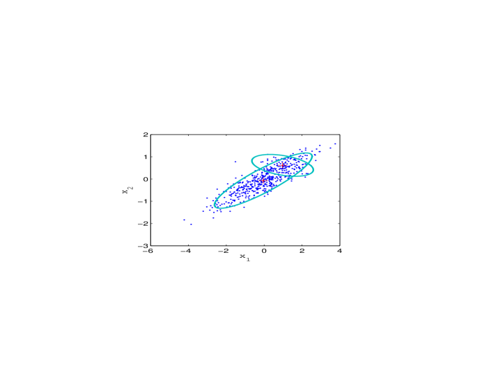
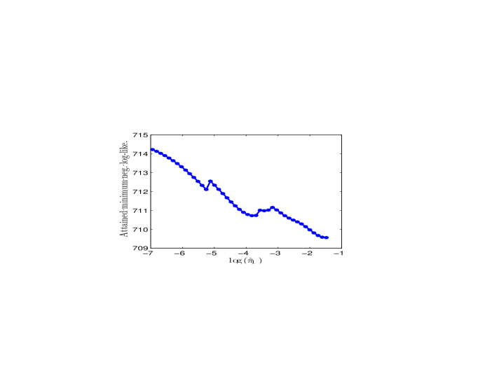
(a)	(b)

Figure 1: An illustration on the behavior of the negative log-likelihood function when a mixing probability is close to zero. (a) The simulated data set and a learned two-component GMM model. (b) The minimized negative log-likelihood as a function of $\log{{\pi}_{1}}$. Note that the $x$-axis is in $\log$ scale.

By the discussion above, we know that $L_{1}$-type penalized likelihood methods are not omnipotent, especially when the model is not a regular statistical model. In fact, the expected complete-data log-likelihood function (2.2) suggests that we need to consider some types of penalties on $\log\pi_{m}$ in order to achieve the sparsity for $\mbox{\boldmath$\pi$}=\{\pi_{1},\cdots,\pi_{M}\}$. In particular, we simply choose to penalize $\log(\frac{\epsilon+\pi_{m}}{\epsilon})=\log(\epsilon+\pi_{m})-\log(\epsilon)$, where $\epsilon$ is a very small positive number, say $10^{-6}$ or $o(n^{-\frac{1}{2}}\log^{-1}n)$ as the discussion of Theorem 3.2. Note that $\log(\epsilon+\pi)-\log(\epsilon)$ is a monotonically increasing function of $\pi$, and it is shrunk to zero when the mixing weight $\pi$ goes to zero. Therefore, we propose the following penalized log-likelihood function,

$$\ell_{P}(\mbox{\boldmath$\theta$})=\ell(\mbox{\boldmath$\theta$})-n\lambda D_{f}\sum_{m=1}^{M}\left[\log(\epsilon+\pi_{m})-\log(\epsilon)\right],$$ (2.3)

where $\ell(\mbox{\boldmath$\theta$})$ is the log-likelihood function, $\lambda$ is a tuning parameter, and $D_{f}$ is the number of free parameters for each component. For GMM with arbitrary covariance matrices, each component has $D_{f}=1+d+d(d+1)/2=d^{2}/2+3d/2+1$ number of free parameters. Although here $D_{f}$ is a constant and can be removed from the equation above, it would simplify the search range of $\lambda$ in the numerical study.

Note our penalty function is similar to that derived with the Dirichlet prior from Bayesian point of view, both using logarithm function of the mixing weights of the finite mixture model as the penalty function or prior distribution function. However, for the Dirichlet prior, the objective penalized likelihood function penalizes $\log\pi_{i}$, and unlike our proposed penalty function $\log(\epsilon+\pi_{m})-\log(\epsilon)$, zero is not in the support area of the penalty function $\log\pi_{i}$. In the mathematical sense, these Bayesian approaches can not shrink the mixing weights to zero exactly since zero is not well defined for the objective function. In other words, the objective function is not continuous when some of mixing weights shrunk continuously to zero. As the discussion by Fan and Li (2001), such discontinuity poses challenges to investigate the statistical properties of related penalized or Bayesian methods. It is be one of main reasons why there is little literature on studies the consistency of the proposed methods based on the Dirichlet prior. Moveover, when $\epsilon=0$, our penalty function can not be seen as in a border family of Dirichlet distributions. In fact, when $\epsilon=0$, there is no definition for the second term of our proposed penalty function. Though when $\epsilon>0$, our proposed penalty function is similar to the one used by Figueirdo and Jain (2002). However, zero is still not in the support area of their proposed improper prior function, and their method has similar problems as those Bayesian approaches based on the Dirichlet prior do.

As discussed in Fan and Li (2001), a good penalty function should yield an estimator with three properties: unbiasedness, sparsity, and continuity. It is obvious that $\log(\frac{\epsilon+\pi_{m}}{\epsilon})$ would over penalize large $\pi_{m}$ and yield a biased estimator. Hence, we also consider the following penalized log-likelihood function,

$$\ell_{P}(\mbox{\boldmath$\theta$})=\ell(\mbox{\boldmath$\theta$})-n\lambda D_{f}\sum_{m=1}^{M}\left[\log(\epsilon+p_{\lambda}(\pi_{m}))-\log(\epsilon)\right].$$ (2.4)

Compared to (2.3), the only difference is that $\pi_{m}$ is replaced by $p_{\lambda}(\pi_{m})$ in the penalty function, where $p_{\lambda}(\pi)$ is the SCAD penalty function proposed by Fan and Li (2001) and is conveniently characterized through its derivative:

$$p^{\prime}_{\lambda}(\pi)=I(\pi\leq\lambda)+\frac{(a\lambda-\pi)_{+}}{(a-1)\lambda}I(\pi>\lambda),$$

for some $a>2$ and $\pi>0$. It is easy to see that, for a relatively large $\pi_{m}$ and $\pi_{m}>a\lambda$, $p_{\lambda}(\pi_{m})$ is a constant, and henceforth the estimator of this $\pi_{m}$ is expected be unbiased.

2.2 Modified EM Algorithm

Here we propose a modified EM algorithm to maximize (2.3) and (2.4) iteratively in two steps.

First we introduce a modified EM algorithm to maximize (2.3). By (2.2) and (2.3), the expected penalized log-likelihood function is

$$\sum_{i=1}^{n}\sum_{m=1}^{M}h_{im}\log\pi_{m}+\sum_{i=1}^{n}\sum_{m=1}^{M}h_{im}\log\phi(\mbox{\bf x}_{i};\mbox{\boldmath$\mu$}_{m},\mbox{\boldmath$\Sigma$}_{m})-n\lambda D_{f}\sum_{m=1}^{M}\left[\log(\epsilon+\pi_{m})-\log(\epsilon)\right].$$ (2.5)

In the E step, we calculate the posterior probability given the current estimate $\widehat{\mbox{\boldmath$\theta$}}=(\widehat{}\mbox{\boldmath$\mu$}_{1},\widehat{}\mbox{\boldmath$\Sigma$}_{1},\ldots,$ $\widehat{}\mbox{\boldmath$\mu$}_{M},\widehat{}\mbox{\boldmath$\Sigma$}_{M},\widehat{\pi}_{1},\ldots,\widehat{\pi}_{M})$

$$h_{im}=\frac{\widehat{\pi}_{m}\phi(\mbox{\bf x}_{i};\widehat{}\mbox{\boldmath$\mu$}_{m},\widehat{}\mbox{\boldmath$\Sigma$}_{m})}{\sum_{m=1}^{M}\widehat{\pi}_{m}\phi(\mbox{\bf x}_{i};\widehat{}\mbox{\boldmath$\mu$}_{m},\widehat{}\mbox{\boldmath$\Sigma$}_{m})}.$$

In the M step, we update $\mbox{\boldmath$\theta$}=\{\mbox{\boldmath$\mu$}_{1},\mbox{\boldmath$\Sigma$}_{1},\cdots,\mbox{\boldmath$\mu$}_{M},\mbox{\boldmath$\Sigma$}_{M},\pi_{1},\cdots,\pi_{M}\}$ by maximizing the expected penalized log-likelihood function (2.5). Note that we can update $\{\pi_{1},\cdots,\pi_{M}\}$ and $\{\mbox{\boldmath$\mu$}_{1},\mbox{\boldmath$\Sigma$}_{1},\cdots,\mbox{\boldmath$\mu$}_{M},\mbox{\boldmath$\Sigma$}_{M}\}$ separately as they are not intervened in (2.5). To obtain an estimate for $\mbox{\boldmath$\pi$}=(\pi_{1},\cdots,\pi_{M})$, we introduce a Lagrange multiplier $\beta$ to take into account for the constraint $\sum_{m=1}^{M}\pi_{m}=1$, and aim to solve the following set of equations,

$$\frac{\partial}{\partial\pi_{m}}\left[\sum_{i=1}^{n}\sum_{m=1}^{M}h_{im}\log\pi_{m}-n\lambda D_{f}\sum_{m=1}^{M}\log(\epsilon+\pi_{m})-\beta(\sum_{m=1}^{M}\pi_{m}-1)\right]=0.$$

Given $\epsilon$ is very close to zero, by straightforward calculations, we obtain

$$\widehat{\pi}_{m}=\max\left\{0,\frac{1}{1-M\lambda D_{f}}\left[\frac{1}{n}\sum_{i=1}^{n}h_{im}-\lambda D_{f}\right]\right\}.$$ (2.6)

The update equations on $\{\mbox{\boldmath$\mu$}_{1},\mbox{\boldmath$\Sigma$}_{1},\cdots,\mbox{\boldmath$\mu$}_{M},\mbox{\boldmath$\Sigma$}_{M}\}$ are the same as those of the standard EM algorithm for GMM (McLachlan and Peel, 2000). Specifically, we update $\mbox{\boldmath$\mu$}_{m}$ and $\mbox{\boldmath$\Sigma$}_{m}$ as follows,

$$\widehat{}\mbox{\boldmath$\mu$}_{m}=\sum_{i=1}^{n}h_{im}\mbox{\bf x}_{i}/\sum_{i=1}^{n}h_{im},\qquad\widehat{}\mbox{\boldmath$\Sigma$}_{m}=\sum_{i=1}^{n}h_{im}(\mbox{\bf x}_{i}-\widehat{}\mbox{\boldmath$\mu$}_{m})(\mbox{\bf x}_{i}-\widehat{}\mbox{\boldmath$\mu$}_{m})^{T}/\sum_{i=1}^{n}h_{im}.$$

In summary the proposed modified EM algorithm works as follows: it starts with a pre-specified large number of components, and whenever a mixing probability is shrunk to zero by (2.6), the corresponding component is deleted, thus fewer components are retained for the remaining EM iterations. Here we abuse the notation $M$ for the number of components at beginning of each EM iteration, and through the updating process, $M$ becomes smaller and smaller. For a given EM iteration step, it is possible that none, one, or more than one components are deleted.

The modified EM algorithm for maximizing (2.4) is similar to the one for (2.3), and the only difference is in the M step for maximizing $\pi$. Given the current estimate $(\pi_{1}^{0},\ldots,\pi_{M}^{0})$ for $\pi$, to solve

$$\frac{\partial}{\partial\pi_{m}}\left[\sum_{i=1}^{n}\sum_{m=1}^{M}h_{im}\log\pi_{m}-n\lambda D_{f}\sum_{m=1}^{M}\log(\epsilon+p_{\lambda}(\pi_{m}))-\beta(\sum_{m=1}^{M}\pi_{m}-1)\right]=0,$$

we substitute $\log(\epsilon+p_{\lambda}(\pi_{m}))$ by its linear approximation $\log(\epsilon+p_{\lambda}(\pi^{0}_{m}))+\frac{p_{\lambda}^{\prime}(\pi_{m}^{0})}{\epsilon+p_{\lambda}(\pi^{0}_{m})}(\pi_{m}-\pi_{m}^{0})$ in the equation above. Then by straightforward calculations, $\pi_{m}$ can be updated as follows

$$\pi_{m}=\frac{1}{T_{m}}\sum\limits_{i=1}^{n}h_{mi}$$ (2.7)

where

$$T_{m}=n-n\lambda D_{f}\sum\limits_{m=1}^{M}\frac{p_{\lambda}^{\prime}(\pi_{m}^{0})\pi_{m}^{0}}{\epsilon+p_{\lambda}(\pi^{0}_{m})}+n\lambda D_{f}\frac{p_{\lambda}^{\prime}(\pi_{m}^{0})}{\epsilon+p_{\lambda}(\pi^{0}_{m})}.$$

If an updated $\pi_{m}$ is smaller than a pre-specified small threshold value, we then set it to zero and remove the corresponding component from the mixture model. In numerical study, (2.7) is seldom exactly equal to zero. Using such threshold method to set mixing weight to zero is only to avoid the numerical unstabilities. Because of the consistent properties of such penalty function derived in Section 3, we can set this pre-specified small threshold value as small as possible, though small threshold value would increase iterative steps of EM algorithm and computation time. In our numerical studies, we set this threshold as $10^{-4}$, but the smallest mixing weight in the following two numerical examples are $1/600$ and $1/1000$, both larger than this threshold.

2.3 Selection of Tuning Parameters

To obtain the final estimate of the mixture model by maximizing (2.3) or (2.4), one needs to select the tuning parameters $\lambda$ and $a$ (the latter is involved (2.4)). Our simulation studies show that the numerical results are not sensitive to the selection of $a$ and therefore by the suggestion of Fan and Li (2001) we set $a=3.7$. For standard LASSO and SCAD penalized regressions, there are many methods to select $\lambda$, such as generalized cross-validation (GCV) and BIC (See Fan and Li, 2001 and Wang et al., 2007). Here we define a BIC value

$$\mathrm{BIC}(\lambda)=\sum\limits_{i=1}^{n}\log\left\{\sum_{m=1}^{\widehat{M}}\pi_{m}\phi(\mbox{\bf x}_{i};\widehat{\mbox{\boldmath$\mu$}}_{m},\widehat{\mbox{\boldmath$\Sigma$}}_{m})\right\}-\frac{1}{2}\widehat{M}D_{f}\log n$$

and select $\widehat{\lambda}$ by

$$\widehat{\lambda}=\mbox{arg}\max\limits_{\lambda}\mbox{BIC}(\lambda),$$

where $\widehat{M}$ is the estimate of the number of components and $\widehat{\mbox{\boldmath$\mu$}}_{m}$ and $\widehat{\mbox{\boldmath$\Sigma$}}_{m}$ are the estimates of $\mbox{\boldmath$\mu$}_{m}$ and $\mbox{\boldmath$\Sigma$}_{m}$ for maximizing $(\ref{e2.3})$ or $(\ref{e2.4})$ for a given $\lambda$.

3 Asymptotic Properties

It is possible to extend our proposed model selection method to more generalized mixture models, However, to illustrate the basic idea of the proposed method without many mathematical difficulties, in this section, we only show the model selection consistency of the proposed method for Gaussian mixture models.

First, we assume that, for the true Gaussian mixture model, there are $q$ mixture components, $q\leq M$ with $\pi_{i}=0$, for $i=1,\ldots,M-q$, $\pi_{i}=\pi^{0}_{l}$, for $i=M-q+1,\ldots,M,l=1,\ldots,q$. Then by the idea of locally conic models (Dacunha-Castelle and Gassiat, 1997 and 1999), the density function of the Gaussian mixture model can be rewritten as

$$f(\mbox{\bf x},\mbox{\boldmath$\theta$})=f(\mbox{\bf x},\theta,\mbox{\boldmath$\beta$})=\sum\limits^{M-q}_{i=1}\lambda_{i}\theta\cdot\phi(\mbox{\boldmath$\mu$}_{i},\mbox{\boldmath$\Sigma$}_{i})+\sum\limits_{l=1}^{q}(\pi_{l}^{0}+\rho_{l}\theta)\cdot\phi(\mbox{\boldmath$\mu$}^{0}_{l}+\theta\delta_{\mu}^{l},\mbox{\boldmath$\Sigma$}_{l}^{0}+\theta\delta_{\Sigma}^{l}).$$

where

$$\mbox{\boldmath$\beta$}=(\lambda_{1},\ldots,\lambda_{M-q},\mbox{\boldmath$\mu$}_{1},\ldots,\mbox{\boldmath$\mu$}_{M-q},\mbox{\boldmath$\Sigma$}_{1},\ldots,\mbox{\boldmath$\Sigma$}_{M-q},\delta_{\mu}^{1},\ldots,\delta_{\mu}^{q},\delta_{\Sigma}^{1},\ldots,\delta_{\Sigma}^{q},\rho_{1},\ldots,\rho_{q}),$$

$\mbox{\boldmath$\mu$}^{0}_{i},i=1,\ldots,q,$ and $\mbox{\boldmath$\Sigma$}_{i}^{0},i=1,\ldots,q,$ are the true values of multivariate normal components, and $(\pi_{1},\ldots,\pi_{M})$ in the original Gaussian mixture model can be defined as $\pi_{i}=\lambda_{i}\theta,i=1,\ldots,M-q$ and $\pi_{i}=\pi_{l}^{0}+\rho_{l}\theta,i=M-q+1,\ldots,M,l=1,\ldots,q$. Similar to Dacunha-Castelle and Gassiat (1997, 1999), by the restrictions imposed on the $\beta$:

$$\lambda_{i}\geq 0,\ \mu_{i}\in\mathbf{R}^{d}, \mbox{\boldmath$\Sigma$}_{i}\in\mathbf{R}^{d\times d},i=1,\ldots,M-q,$$ and

$$\delta_{\mu}^{l}\in\mathbf{R}^{d},\ \delta_{\Sigma}^{l}\in\mathbf{R}^{d\times d}, \rho\in\mathbf{R},\ l=1,\ldots,q,$$ and

$$\sum\limits_{i=1}^{M-q}\lambda_{i}+\sum\limits_{l=1}^{q}\rho_{l}=0 \sum\limits_{i=1}^{M-q}\lambda_{i}^{2}+\sum\limits_{l=1}^{q}\rho_{l}^{2}+\sum\limits_{l=1}^{q}\|\delta^{l}_{\mu}\|^{2}+\sum\limits_{l=1}^{q}\|\delta^{l}_{\Sigma}\|^{2}=1,$$ and

and by the permutation, such a parametrization is locally conic and identifiable.

After the parametrization, the penalized likelihood functions (2.3) and (2.4) can be written as

$$\ell_{P}(\mbox{\boldmath$\theta$}) = \ell(\mbox{\boldmath$\theta$})-n\lambda D_{f}\sum_{m=1}^{M}\left[\log(\epsilon+\pi_{m}))-\log(\epsilon)\right]$$ (3.1)

$$\widehat{=} \ell_{P}(\theta,\mbox{\boldmath$\beta$})$$

$$= \sum\limits_{i=1}^{n}\log f(\mbox{\bf x}_{i},\theta,\mbox{\boldmath$\beta$})-n\lambda D_{f}\sum_{m=1}^{M}\left[\log(\epsilon+\pi_{m})-\log(\epsilon)\right],$$

and

$$\ell_{P}(\mbox{\boldmath$\theta$}) = \ell(\mbox{\boldmath$\theta$})-n\lambda D_{f}\sum_{m=1}^{M}\left[\log(\epsilon+p_{\lambda}(\pi_{m}))-\log(\epsilon)\right]$$ (3.2)

$$\widehat{=} \ell_{P}(\theta,\mbox{\boldmath$\beta$})$$

$$= \sum\limits_{i=1}^{n}\log f(\mbox{\bf x}_{i},\theta,\mbox{\boldmath$\beta$})-n\lambda D_{f}\sum_{m=1}^{M}\left[\log(\epsilon+p_{\lambda}(\pi_{m}))-\log(\epsilon)\right],$$

respectively.

We need the following conditions to derive the asymptotic properties of our proposed method.

• $\|\mu_{i}\|\leq C_{1},\|\mbox{\boldmath$\Sigma$}_{i}\|\leq C_{2},i=1,\ldots,M,$ where $C_{1}$ and $C_{2}$ are large enough constants.

• $\min\limits_{i,k}\{\lambda_{k}(\mbox{\boldmath$\Sigma$}_{i}),k=1,\ldots,d,i=1,\ldots,M\}\geq C_{3}$, where $\lambda_{k}(\mbox{\boldmath$\Sigma$}_{i})$ are the eigenvalues of $\mbox{\boldmath$\Sigma$}_{i}$ and $C_{3}$ is a positive constant.

Compared to the conditions in Dacunha-Castelle and Gassiat (1997, 1999), the conditions P1 and P2 are slightly stronger. Without lose of generality, we assume that the parameters in the mixture model are in a bounded compact space not only for mathematical conveniences, but also for avoiding the identifiability and ill-posedness problems of the finite mixture model as discussed in Bishop (2006). Those conditions are also practically reasonable for our revised EM algorithm as the discussion in Figueirdo and Jain (2002).

First, even if it is known there is $K$ mixture components in the model, the maximum likelihood or penalized maximum likelihood solution still has a total of $K!$ equivalent solutions corresponding to the $K!$ ways of assigning $K$ sets of parameters to $K$ components. Although this is an important issue when we wish to interpret the estimate parameter values for a selected model. However, the main focus of our paper is to determine the order and find a good density estimate with the finite mixture model. The identifiability problem is irrelevant as all equivalent solutions have same estimate of the order and the density function.

Second, Condition (P2) is imposed to guarantee the non-singularity of the covariance matrices, avoiding the ill-posedness in the estimation of the finite multivariate Gaussian mixture model with unknown covariance matrices using our proposed penalized maximum likelihood method. Similar as the discussion in Figueirdo and Jain (2002), given a sufficient large number of the initial mixture components, say M, our proposed modified EM algorithm selects components in a backwards manner by merging smaller components into a large component, and thus reducing the number of components. On the other hand, pre-specifying an extreme large value for M should be avoided as well. In our numerical studies, the initial number of mixture components M is set to be smaller than n/p so that each estimated mixture component has a positive covariance matrix, as required by Condition (P2).

Theorem 3.1

Under the conditions (P1) and (P2) and if $\sqrt{n}\lambda\to\infty$, $\lambda\to 0$ and $\epsilon=o(1/\sqrt{n})$, there exists a local maximizer $(\theta,\mbox{\boldmath$\beta$})$ of $\ell_{P}$, which was given in (3.2), such that $\theta=O_{p}(1/\sqrt{n})$, and for such local maximizer, the number of the mixture components $\widehat{q}_{n}\to q$ with probability tending to one.

Theorem 3.2

Under the conditions (P1) and (P2) and if $\sqrt{n}\lambda\to C$ and $\epsilon=o(\frac{1}{\sqrt{n}\log n})$ where $C$ is a constant, there exists a local maximizer $(\theta,\mbox{\boldmath$\beta$})$ of $\ell_{P}$, which was given in (3.1), such that $\theta=O_{p}(1/\sqrt{n})$, and for such local maximizer, the number of the mixture components $\widehat{q}_{n}\to q$ with probability tending to one.

Remarks: Under Conditions (P1) and (P2) and with an appropriate tuning parameter $\lambda$, the consistency of our proposed two penalized methods have been shown by the two theorems above. Although maximizing (3.2) using our proposed EM algorithm is a bit complicated than that for (3.1), it has theoretical advantages. Unlike (3.2), a mixture component with a relative large mixing weight $\pi_{i}$ is still penalized in (3.1) by the penalty function $\log(\pi_{i}+\epsilon)-\log\epsilon$, and this would produce a bias model estimation and affect the consistency of the model selection as the discussion by Fan and Li (2001). Moreover, in practice it is easier to select an appropriate tuning parameter for (3.2) than for (3.1) to guarantee the consistency of the final model selection and estimation. In particular, the following theorem shows that the proposed BIC criterion always selects the reasonable tuning parameter with probability tending one by which maximizing (3.2) selects the consistent component number of the finite Gaussian mixture model.

Let $\mathrm{Component}_{\lambda}$ denote the number of component of Gaussian mixture models selected by (3.2) with the tuning parameter $\lambda$, and $\lambda_{BIC}$ is the lambda selected by the proposed BIC criterion in Section 2.3. Then we have the following theorem.

Theorem 3.3

Under the conditions (P1) and (P2), $\mathrm{Pr}(\mathrm{Component}_{\lambda_{BIC}}=q)\to 1$.

The proofs of the theorems are given in the appendix.

4 Numerical Studies

4.1 Example I

In the first example, we generate 600 samples from a three-component bivariate normal mixture with mixing weights $\pi_{1}=\pi_{2}=\pi_{3}=1/3$, mean vectors $\mbox{\boldmath$\mu$}_{1}=\left[-1,1\right]^{T}$, $\mbox{\boldmath$\mu$}_{2}=\left[1,1\right]^{T}$, $\mbox{\boldmath$\mu$}_{3}=\left[0,-\sqrt{2}\right]^{T}$, and covariance matrices $\mbox{\boldmath$\Sigma$}_{1}=[0.65,~{}0.7794;~{}0.7794,~{}1.55]$, $\mbox{\boldmath$\Sigma$}_{2}=[0.65,-0.7794;~{}-0.7794,~{}1.55]$, $\mbox{\boldmath$\Sigma$}_{3}=\text{diag}\{2,0.2\}$. In fact, these three components are obtained by rotating and shifting a common Gaussian density $\mathcal{N}(\mbox{\boldmath{0}},\textrm{diag}(2,0.2))$, and together they exhibit a triangle shape.

We run both of our proposed penalized likelihood methods (2.3) and (2.4) for 300 times. The maximum initial number of components is set to be 10 or 50 , the initial value for the modified EM algorithms is estimated by K-means clustering, and the tuning parameter $\lambda$ is selected by our proposed BIC method. Figure 2 shows the evolution of the modified EM algorithm, with the maximum number of components as 10. We compare our proposed methods with traditional AIC and BIC methods. Figure 3(a-c) shows the histograms of the estimated component numbers. One can see that our proposed methods perform much better in identifying the correct number of components than AIC and BIC methods do. In fact, both proposed methods estimate the number of components $100\%$ correctly regardless of the maximum initial number of components. Figure 3(d) depicts the evolution of the penalized log-likelihood function (2.3) for the simulated data set in Figure 2(a) in one run, and shows how our proposed modified EM algorithm converges numerically.

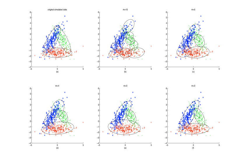
Figure 2: One typical run. (a) a simulated data set. (b) initialization for $m=10$ components, (c-e) three intermediate estimates for $M=6,5,4$, respectively, (f) the final estimate for $M=3$.

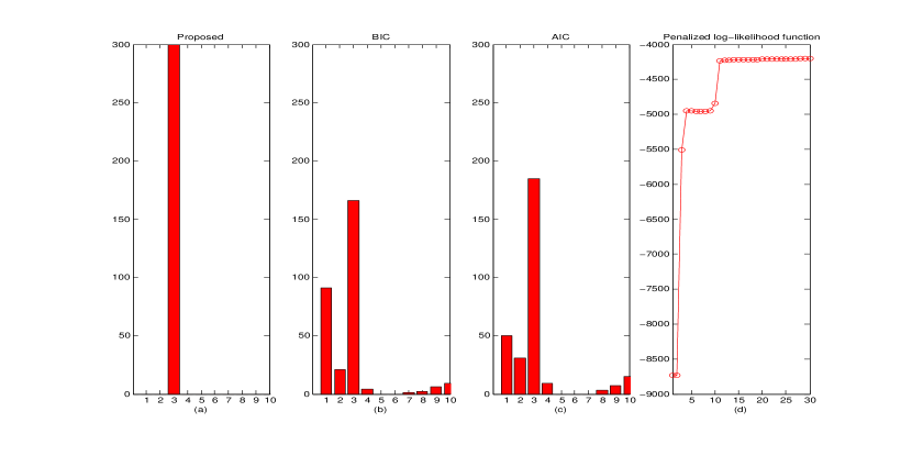
Figure 3: Histogram of estimated numbers of components. (a) the proposed method (2.3), (b) BIC, (c) AIC. (d) The penalized log likelihood function for one typical run.

In addition, when the number of components is correctly identified, we summarize the estimation of the unknown parameters of Gaussian distributions and mixing weights in Table 1 and Table 2 with different maximum initial number of components. For the covariance matrix, we use eigenvalues because the three components have the same shape as $\mathcal{N}(\mbox{\boldmath{0}},\textrm{diag}(2,0.2))$. Table 1 and Table 2 show that the modified EM algorithms give accurate estimate for parameters and mixing weights. The final estimate of these parameters is robust to the initialization of the maximum number of components.

Table 1: Parameter Estimation (The initial number of components $M=10$)

Component		Mixing Probability	Mean		Covariance (eigenvalue)
1	True	0.3333	-1	1	2	0.2
	(2.3)	0.3342(.0201)	-0.9911(.0861)	1.0169(.1375)	2.0034(.3022)	0.1981(.0264)
	(2.4)	0.3356(.0187)	-1.0022 (.0875)	1.0007(.1428)	2.0205(.2769)	0.1973 (.0265)
2	True	0.3333	1	1	2	0.2
	(2.3)	0.3317(.0196)	1.0151(.0845)	0.9849(.1318)	1.9794(.2837)	0.1977(.0303)
	(2.4)	0.3321 (.0193)	1.0108(.0790)	0.9904(.1253)	1.9825(.2980)	0.1957 (.0292)
3	True	0.3333	0	-1.4142	2	0.2
	(2.3)	0.3341(.0171)	0.0019(.1324)	-1.4112(.0405)	1.9722(.2425)	0.1973(.0258)
	(2.4)	0.3322(.0159)	0.0014(.1449)	-1.4103(.0404)	1.9505(.2424)	0.1978(.0267)

Table 2: Parameter Estimation (The initial number of components $M=50$)

Component		Mixing Probability	Mean		Covariance (eigenvalue)
1	True	0.3333	-1	1	2	0.2
	(2.3)	0.3342(.0201)	-1.0080(.0881)	0.9854(.1372)	1.9603(.2857)	0.1974(.0296)
	(2.4)	0.3320(.0190)	-1.0017 (.0859)	0.9985(.1389)	1.9604(.2830)	0.1960 (.0286)
2	True	0.3333	1	1	2	0.2
	(2.3)	.3347(.0170)	0.9879(.0885)	1.0166(.1385)	1.9531(.2701)	0.1981(.0283)
	(2.4)	0.3345 (.0182)	0.9987(.0896)	1.0044(.1402)	1.9661(.2460)	0.1971 (.0248)
3	True	0.3333	0	-1.4142	2	0.2
	(2.3)	0.3329(.0198)	0.0210(.1329)	-1.4105(.0344)	1.9717(.2505)	0.1975(.0265)
	(2.4)	0.3334(.0164)	0.0117(.1302)	-1.4116(.0372)	1.9736(.2769)	0.1998(.0281)

4.2 Example II

In the second example, we consider a situation where the mixture components overlap and may have same means but different covariance matrices. This is a rather challenging example, and the proposed method by Chen and Khalili (2008) can not be applied as some components have the same mean. Specifically, we generate 1000 samples with mixing weights $\pi_{1}=\pi_{2}=\pi_{3}=0.3$, $\pi_{4}=0.1$, mean vectors $\mbox{\boldmath$\mu$}_{1}=\mbox{\boldmath$\mu$}_{2}=\left[-2,-2\right]^{T}$, $\mbox{\boldmath$\mu$}_{3}=\left[2,0\right]^{T}$, $\mbox{\boldmath$\mu$}_{4}=\left[1,-4\right]^{T}$, and

$$\mbox{\boldmath$\Sigma$}_{1} =\left[\begin{array}[]{cc}0.1&0\\ 0&0.2\end{array}\right],\qquad\mbox{\boldmath$\Sigma$}_{2} =\left[\begin{array}[]{cc}2&2\\ 2&7\end{array}\right],$$

$$\mbox{\boldmath$\Sigma$}_{3} =\left[\begin{array}[]{cc}0.5&0\\ 0&4\end{array}\right],\qquad\mbox{\boldmath$\Sigma$}_{4} =\left[\begin{array}[]{cc}0.125&0\\ 0&0.125\end{array}\right].$$

Similar to the first Example, we run our proposed methods for 300 times. The maximum number of components is set to be 10 or 50, the initial value for the modified EM algorithms is estimated by K-means clustering, and the tuning parameter $\lambda$ is selected by our proposed BIC method. Figure 4 shows the evolution of the modified EM algorithm for (2.3) with the maximum initial number of components as 10 for one simulated data set. Figure 5 shows that our proposed method can identify the number of components $100\%$ correctly, and performs much better than AIC and BIC methods. Table 3 and Table 4 show that the modified EM algorithms give accurate estimates for parameters and mixing weights. Similar as the first example, the final estimate of these parameters is robust to the initialization of the maximum number of components.

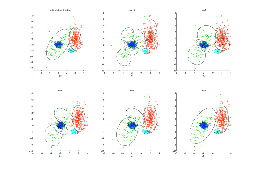
Figure 4: One typical run. (a) a simulated data set. (b) initialization for $M=10$ components, (c-e) three intermediate estimates for $M=7,6,5$, respectively, (f) the final estimate for $M=4$.

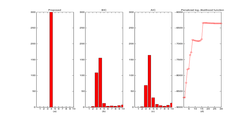
Figure 5: Histogram of estimated numbers of components. (a) the proposed method (2.3), (b) BIC, (c) AIC. (d) The penalized log likelihood function for one typical run.

Table 3: Parameter Estimation (The initial number of components $M=10$)

Component		Mixing Probability	Mean		Covariance (eigenvalue)
1	True	0.3	-2	-2	0.1	0.2
	(2.3)	0.3022(.0093)	-2.0010(.0216)	-1.9989(.0291)	0.0979(.0114)	0.2010 (.0242)
	(2.4)	0.3009(.0095)	-1.9995(.0206)	-1.9975(.0319)	0.0990(.0119)	0.2003(.0226)
2	True	0.3	-2	-2	1.2984	7.7016
	(2.3)	0.2995(.0112)	-1.9989(.1133)	-1.9963(.1837)	1.2864(.1407)	7.7219(.7301)
	(2.4)	0.3017(.0118)	-1.9995(.1202)	-2.0049(.1811)	1.2926(.1343)	7.5856(.7301)
3	True	0.3	2	0	0.5	4
	(2.3)	0.3019(.0083)	1.9943(.0483)	0.0001(.1294)	0.4986(.0529)	3.9951(.3496)
	(2.4)	0.3012(.0087)	1.9995(.0511)	-0.0001(.1244)	0.4963(.0544)	3.9998(.3911)
4	True	0.1	1	-4	0.125	0.125
	(2.3)	0.0964(.0038)	1.0005(.0373)	-3.9966(.0394)	0.1143(.0245)	0.1339(.0252)
	(2.4)	0.0962(.0047)	0.9993(.0394)	-4.0013(.0417)	0.1167(.0259)	0.1317(.0278)

Table 4: Parameter Estimation (The initial number of components $M=50$)

Component		Mixing Probability	Mean		Covariance (eigenvalue)
1	True	0.3	-2	-2	0.1	0.2
	(2.3)	0.3016(.0107)	-1.9982(.0223)	-1.9998(.0312)	0.0986(.0110)	0.2034 (.0241)
	(2.4)	0.3009(.0095)	-1.9986(.0218)	-1.9978(.0320)	0.0993(.0110)	0.2010(.0238)
2	True	0.3	-2	-2	1.2984	7.7016
	(2.3)	0.3002(.0128)	-2.0040(.1086)	-2.0052(.1819)	1.2823(.1386)	7.6696(.7538)
	(2.4)	0.3017(.0115)	-1.9988(.1173)	-2.0116(.1811)	1.2757(.1318)	7.6734(.7476)
3	True	0.3	2	0	0.5	4
	(2.3)	0.3015(.0083)	1.9986(.0500)	0.0054(.1365)	0.4998(.0531)	3.9951(.3651)
	(2.4)	0.3012(.0084)	2.0015(.0505)	0.0102(.1268)	0.4915(.0524)	3.9751(.3770)
4	True	0.1	1	-4	0.125	0.125
	(2.3)	0.0966(.0044)	0.9983(.0408)	-4.0019(.0431)	0.1150(.0251)	0.1327(.0258)
	(2.4)	0.0962(.0050)	1.0011(.0402)	-4.0019(.0425)	0.1154(.0256)	0.1313(.0254)

4.3 Real Data Analysis

We apply our proposed methods to an image segmentation data set at UCI Machine Learning Repository (http://archive.ics.uci.edu/ml/datasets/Image+Segmentation). This data set was created from a database of seven outdoor images (brickface, sky, foliage, cement, window, path and grass). Each image was hand-segmented into instances of $3\times 3$ regions, and 230 instances were randomly drawn. For each instance, there are 19 attributes. We here only focus on four images, brickface, sky, foliage and grass, and two attributes, extra red and extra green. Our objective is to estimate the joint probability density function of the two attributes (See Figure 6(a)) using a Gaussian mixture with arbitrary covariance matrices. In other words, we implement our proposed method to identify the number of components, and to simultaneously estimate the unknown parameters of bivariate normal distributions and mixing weights. Although we consider only four images, Figure 6(a) suggests that a five-component Gaussian mixture is more appropriate and the brickface image is better represented by two components.

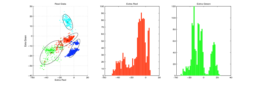
(a)                                  (b)                                (c)

Figure 6: (a) Scatter plot of scaled real data. Brickface (blue), Sky (green), Foliage (red), Grass (light blue); (b-c) Histograms of marginal density. (b) Extra red, and (c) Extra green.

As in the simulation studies, we run our proposed method for 300 times. For each run, we randomly draw 200 instances for each images. The maximum number of components is set to be ten, and the initial value for the modified EM algorithm is estimated by the K-means clustering. Because there is little difference between numerical results of the two proposed methods (2.3) and (2.4), here we only show the numerical results obtained by maximizing (2.3). Figure 7 shows the evolution of the modified EM algorithm for one run. Figure 8 shows that our proposed method selects five components with high probability. For a five-component Gaussian mixture model, we summarize the estimation of parameters and mixing weights in Table 5.

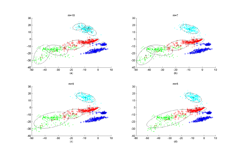
Figure 7: One typical run. (a) Initialization with $M=10$ components, (b) and (c) two intermediate estimates for $M=7$ and $M=6$, respectively, (d) the final estimate $M=5$.

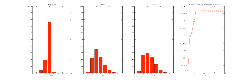
Figure 8: Histogram of estimated numbers of components. (a) the proposed method (2.3), (b) BIC, (c) AIC. (d) The penalized log likelihood function for one typical run.

Table 5: Parameter Estimation, $\widehat{M}=5$

Component	Underlying	Mixing Probability	Mean		Standard Deviation
			(Ex-red, Ex-green)		(Ex-red, Ex-green)
1	Sky & Foliage	.4153(0.0555)	-27.7689(2.3336)	-13.7343(1.1377)	12.0464(1.1726)	7.3739(0.3745)
2	Grass	.2617(0.0523)	-9.3724(0.8588)	13.4992(4.0740)	3.6393(1.2160)	3.5632(1.3567)
3	Foliage & Brickface	.1447(0.0425)	-4.9511(1.3913)	-3.3625(3.5537)	3.1584(0.7102)	1.6728(0.4004)
4	Brickface	.0824(0.0487)	-1.3474(0.8417)	-12.0906(7.2158)	2.5780(1.5227)	1.3302(0.7854)
5	Brickface	.0936(0.0717)	3.5476(1.4703)	-8.4996(2.1980)	1.5110(1.2288)	1.3293(1.6460)

5 Conclusions and Discussions

In this paper, we propose a penalized likelihood approach for multivariate finite Gaussian mixture models which integrates model selection and parameter estimation in a unified way. The proposed method involves light computational load and is very attractive when there are many possible candidate models. Under mild conditions, we have, both theoretically and numerically, shown that our proposed method can select the number of components consistently for Gaussian mixture models. Though we mainly focus on Gaussian mixture models, we believe our method can be extended to more generalized mixture models. This requires more rigorous mathematical derivations and further theoretical justifications, and is beyond the scope of this paper.

In practice, our proposed modified EM algorithm gradually discards insignificant components, and does not generate new components or split any large components. If necessary, for very complex problems, one can perform the split-and-merge operations (Ueda et al.. 1999) after certain EM iterations to improve the final results. We only show the convergence of our proposed modified EM algorithm through simulations, and further theoretical investigation is needed. Moreover, classical acceleration methods, such as Louis’ method, Quasi-Newton method and Hybrid method (McLachlan and Peel, 2000), may be used to improve the convergence rate of our proposed modified EM algorithm.

Another practical issue is the selection of the tuning parameter $\lambda$ for the penalized likelihood function. We propose a BIC selection method, and simulation results show it works well. Moreover, our simulation results show the final estimate is quite robust to the initial number of components.

In this paper, we propose two penalized log-likelihood functions (2.3) and (2.4). Although the numerical results obtained by these two penalized functions are very similar, we believe they have different theoretical properties. We have shown the consistency of model selection and tuning parameter selection by maximizing (2.4) and the BIC criterion proposed in the paper under mild conditions. We have also shown the consistency of model selection by maximizing (2.3), but we note that the conditions are somewhat restrictive. In particular, the consistency of BIC criterion to select the tuning parameter for (2.3) needs further investigations.

An ongoing work is to investigate how to extend our proposed penalized likelihood method to the mixture of factor analyzers (Ghahramani and Hinton, 1997), and to integrate clustering and dimensionality reduction in a unified way.

Appendix: Proof

We now outline the key ideas of the proof for Theorem 3.1.

First assume the true Gaussian mixture density is

$$g_{0}=\sum\limits_{l=1}^{q}\pi_{l}^{0}\phi(\mbox{\boldmath$\mu$}_{l}^{0},\mbox{\boldmath$\Sigma$}_{l}^{0}),$$

then define $\mathcal{D}$ as the subset of functions of form

$$\sum\limits_{l=1}^{q}\pi_{l}^{0}\sum\limits_{i=1}^{d}\frac{\delta_{\mu_{i}}^{l}D_{i}^{1}\phi(\mbox{\boldmath$\mu$}^{0}_{i},\mbox{\boldmath$\Sigma$}^{0}_{i})}{g_{0}}+\sum\limits_{l=1}^{q}\pi_{l}^{0}\sum\limits_{i\geq j=1}^{d}\frac{\delta_{\Sigma_{i,j}}^{l}D_{i,j}^{1}\phi(\mbox{\boldmath$\mu$}^{0}_{l},\mbox{\boldmath$\Sigma$}^{0}_{l})}{g_{0}}+\sum\limits_{i=1}^{M-q}\lambda_{i}\frac{\phi(\mbox{\boldmath$\mu$}_{i},\mbox{\boldmath$\Sigma$}_{i})}{g_{0}}+\sum\limits_{l=1}^{q}\rho_{l}\frac{\phi(\mbox{\boldmath$\mu$}_{l}^{0},\mbox{\boldmath$\Sigma$}_{l}^{0})}{g_{0}}$$

where $D_{i}^{1}$ is the derivative of $\phi(\mu_{i},\mbox{\boldmath$\Sigma$}_{i})$ for the $i$th component of $\mu_{i}$, $D_{i,j}^{1}$ is the derivative of $\phi(\mu_{i},\mbox{\boldmath$\Sigma$}_{i})$ for the $(i,j)$ component of $\mbox{\boldmath$\Sigma$}_{i}$. For functions in $\mathcal{D}$, $(\mbox{\boldmath$\mu$}_{i},\mbox{\boldmath$\Sigma$}_{i}),i=1,\ldots,M-q$ and $\mbox{\boldmath$\mu$}_{l}^{0},\mbox{\boldmath$\Sigma$}_{l}^{0}$ satisfy the conditions P1 and P2. The important consequence for $\mathcal{D}$ is the following proposition.

Proposition A.1. Under the conditions P1 and P2, $\mathcal{D}$ is a Donsker class.

Proof: First, by the conditions P1 and P2, it is easy to check that the conditions P1 and P2 in Keribin (2000) or P0 and P1 in Dacunha-Castelle and Gassiat (1999) are satisfied by $\mathcal{D}$. Then $(D_{i}^{1}\phi(\mbox{\boldmath$\mu$}^{0}_{i},\mbox{\boldmath$\Sigma$}^{0}_{i}),D_{i,j}^{1}\phi(\mbox{\boldmath$\mu$}^{0}_{l},\mbox{\boldmath$\Sigma$}^{0}_{l}),\phi(\mbox{\boldmath$\mu$}_{i},\mbox{\boldmath$\Sigma$}_{i}))$ are within envelope functions $(F_{1},F_{2},F_{3})$, and square integrable under $g_{0}\nu$. On the other hand, by the restrictions imposed on the $\beta$, $\lambda_{i},\rho_{l},\pi_{l}^{0}\delta_{\mu_{i}}^{l}$ and $\pi_{l}^{0}\delta_{\Sigma_{i}}^{l}$ are bounded. Therefore, similar to the proof of Theorem 4.1 in Keribin (2000) or the proof of Proposition 3.1 in Dacunha-Castelle and Gassiat (1999), it is straightforward to show that $\mathcal{D}$ has the Donsker property with the bracketing number $N(\varepsilon)=1/\varepsilon^{K}$ where $K=M(d+d(d+1)/2)$. $\Box$

Proof of Theorem 3.1: To prove the theorem, we first show that there exists a maximizer $(\theta,\mbox{\boldmath$\beta$})$ such that $\theta=O_{p}(1/\sqrt{n})$. In fact, it is sufficient to show that, for a large constant $C$, $\ell(\theta,\mbox{\boldmath$\beta$})<\ell(0,\mbox{\boldmath$\beta$})$ where $\theta=C/\sqrt{n}$. Let $\theta=C/\sqrt{n}$, and notice that

$$\ell_{p}(\theta,\mbox{\boldmath$\beta$})-\ell_{p}(0,\mbox{\boldmath$\beta$}) = \sum\limits_{i=1}^{n}\{\log f(\mbox{\bf x}_{i},\theta,\mbox{\boldmath$\beta$})-\log g_{0}(\mbox{\bf x}_{i})\}-n\lambda D_{f}\sum\limits_{m=1}^{M}[\log(\epsilon+p_{\lambda}(\pi_{m}))-\log(\epsilon)]$$

$$+n\lambda D_{f}\sum\limits_{l=1}^{q}[\log(\epsilon+p_{\lambda}(\pi^{0}_{l}))-\log(\epsilon)],$$

and then

$$\ell_{p}(\theta,\mbox{\boldmath$\beta$})-\ell_{p}(0,\mbox{\boldmath$\beta$}) \leq \sum\limits_{i=1}^{n}\{\log f(\mbox{\bf x}_{i},\theta,\mbox{\boldmath$\beta$})-\log g_{0}(\mbox{\bf x}_{i})\}$$

$$-n\lambda D_{f}\sum\limits_{m=M-q+1}^{M}[\log(\epsilon+p_{\lambda}(\pi_{m}))-\log(\epsilon+p_{\lambda}(\pi^{0}_{m-M+q}))]$$

$$\widehat{=} I_{1}+I_{2}.$$

For $I_{2}$, because $\theta=C/\sqrt{n}$ and by the restriction condition on $\rho_{l},l=1,\ldots,q$, we have $|\pi_{m}-\pi_{m-M+q}^{0}|\leq C/\sqrt{n}$ when $m>M-q$. Due to the property of the penalty function, we then have

$$|I_{2}| = |-n\lambda D_{f}\sum\limits_{m=M-q+1}^{M}[\log(\epsilon+p_{\lambda}(\pi_{m}))-\log(\epsilon+p_{\lambda}(\pi^{0}_{m-M+q}))]|$$

$$= |-n\lambda D_{f}\sum\limits_{m=M-q+1}^{M}[\log(\epsilon+a\lambda)-\log(\epsilon+a\lambda)]|$$

$$= 0.$$

For $I_{1}$, we have

$$I_{1} = \sum\limits_{i=1}^{n}\frac{f(\mbox{\bf x}_{i},\theta,\mbox{\boldmath$\beta$})-g_{0}(\mbox{\bf x}_{i})}{g_{0}(\mbox{\bf x}_{i})}-\frac{1}{2}\sum\limits_{i=1}^{n}\left(\frac{f(\mbox{\bf x}_{i},\theta,\mbox{\boldmath$\beta$})-g_{0}(\mbox{\bf x}_{i})}{g_{0}(\mbox{\bf x}_{i})}\right)^{2}+\frac{1}{3}\sum\limits_{i=1}^{n}U_{i}\left(\frac{f(\mbox{\bf x}_{i},\theta,\mbox{\boldmath$\beta$})-g_{0}(\mbox{\bf x}_{i})}{g_{0}(\mbox{\bf x}_{i})}\right)^{3}$$

holds for $\theta=C/\sqrt{n}$, where $|U_{i}|\leq 1$. Expand $f(\mbox{\bf x},\theta,\mbox{\boldmath$\beta$})$ up to the second order,

$$f(\mbox{\bf x},\theta,\mbox{\boldmath$\beta$})=g_{0}(\mbox{\bf x})+\theta\cdot f^{\prime}(\mbox{\bf x},0,\mbox{\boldmath$\beta$})+\frac{\theta^{2}}{2}\cdot f^{\prime\prime}(\mbox{\bf x},\theta^{\ast},\mbox{\boldmath$\beta$}),$$

for a $\theta^{\ast}\leq\theta$.

Noticing $\theta=C/\sqrt{n}$, $\mathrm{E}f^{\prime}/g_{0}=0$ and $\mathrm{E}f^{\prime\prime}/g_{0}=0$, and by the conditions P1, P2 and Proposition A.1 for the class $\mathcal{D}$, we have

$$I_{1}=\left\{\sum\limits_{i=1}^{n}\theta\frac{f^{\prime}(\mbox{\bf x}_{i},0,\mbox{\boldmath$\beta$})}{g_{0}(\mbox{\bf x}_{i})}-\frac{1}{2}\sum\limits_{i=1}^{n}\theta^{2}\left(\frac{f^{\prime}(\mbox{\bf x}_{i},0,\mbox{\boldmath$\beta$})}{g_{0}(\mbox{\bf x}_{i})}\right)^{2}\right\}(1+o_{p}(1)).$$

Since $\frac{1}{\sqrt{n}}\sum\limits_{i=1}^{n}\frac{f^{\prime}(\mbox{\bf x}_{i},0,\mbox{\boldmath$\beta$})}{g_{0}(\mbox{\bf x}_{i})}$ converges uniformly in distribution to a Gaussian process by Proposition A.1, and $\sum\limits_{i=1}^{n}\left(\frac{f^{\prime}(\mbox{\bf x}_{i},0,\mbox{\boldmath$\beta$})}{g_{0}(\mbox{\bf x}_{i})}\right)^{2}$ is of order $O_{p}(n)$ by the law of large numbers, we have

$$I_{1}=\frac{C}{\sqrt{n}}\cdot O_{P}(\sqrt{n})-\frac{C^{2}}{n}\cdot O_{p}(n).$$

When $C$ is large enough, the second term of $I_{1}$ dominates other terms in the penalized likelihood ratio. Then we have

$$\ell_{p}(\theta,\mbox{\boldmath$\beta$})-\ell_{p}(0,\mbox{\boldmath$\beta$})<0$$

with probability tending to one. Hence there exists a maximizer $(\theta,\mbox{\boldmath$\beta$})$ with probability tending to one such that

$$\theta=O_{p}(\frac{1}{\sqrt{n}}).$$

Next we show that $\widehat{q}=q$ or that $\widehat{\pi}_{m}=0,m=1,\ldots,M-q$, when the maximizer $(\theta,\mbox{\boldmath$\beta$})$ satisfies $\theta=O_{p}(\frac{1}{\sqrt{n}})$. In fact, when $\theta=O_{p}(\frac{1}{\sqrt{n}})$, we have $\widehat{\pi}_{m}=O_{p}(1/\sqrt{n}),m=1,\ldots,M-q,$ by the restriction condition on $\lambda_{i}$. A Lagrange multiplier $\beta$ is taken into account for the constraint $\sum_{m=1}^{M}\widehat{\pi}_{m}=1$. Then it is then sufficient to show that

$$\frac{\partial\ell^{\ast}(\mbox{\boldmath$\theta$})}{\partial\widehat{\pi}_{m}}<0\quad\mbox{for}\quad\widehat{\pi}_{m}<\varepsilon_{n}$$ (A.1)

with probability tending to one for the maximizer $(\theta,\mbox{\boldmath$\beta$})$ where $\varepsilon_{n}=Cn^{-1/2}$, $m\leq M-q$, and $\ell^{\ast}(\mbox{\boldmath$\theta$})=\ell(\mbox{\boldmath$\theta$})-\beta(\sum_{m=1}^{M}\pi_{m}-1).$ To show the equation above, we consider the partial derivatives for $\widehat{\pi}_{m},\ m>M-q$ firstly. They should satisfy the following equation,

$$\frac{\partial\ell^{\ast}(\mbox{\boldmath$\theta$})}{\partial\widehat{\pi}_{m}}=\sum\limits_{i=1}^{n}\frac{\phi_{m}(\mu_{m},\mbox{\boldmath$\Sigma$}_{m})}{\sum_{i=1}^{M}\widehat{\pi}_{i}\phi_{i}(\mu_{i},\mbox{\boldmath$\Sigma$}_{i})}-n\lambda D_{f}\frac{1}{\epsilon+\widehat{\pi}_{m}}-\beta=0.$$ (A.2)

It is obvious that the first term in the equation above is of order $O_{p}(n)$ by the law of large numbers. If $m>M-q$ and $\theta=O_{p}(\frac{1}{\sqrt{n}})$, it is easy to know that $\widehat{\pi}_{m}=\pi_{m-M+q}^{0}+O_{p}(1/\sqrt{n})>\frac{1}{2}\cdot\min(\pi_{1}^{0},\ldots,\pi_{q}^{0})$, and hence the second term should be $O_{p}(n\lambda)=o_{p}(n)$. So we have $\beta=O_{p}(n)$.

Next, consider

$$\frac{\partial\ell^{\ast}(\mbox{\boldmath$\theta$})}{\partial\widehat{\pi}_{m}}=\sum\limits_{i=1}^{n}\frac{\phi_{m}(\mu_{m},\mbox{\boldmath$\Sigma$}_{m})}{\sum_{i=1}^{M}\widehat{\pi}_{i}\phi_{i}(\mu_{i},\mbox{\boldmath$\Sigma$}_{i})}-n\lambda D_{f}\frac{1}{\epsilon+\widehat{\pi}_{m}}-\beta.$$ (A.3)

where $m\leq M-q$ and $\widehat{\pi}_{m}<\varepsilon_{n}$. As shown for (A.3), it is obvious that the first term and the third term $\beta$ in the equation above are of order $O_{p}(n)$. For the second term, because $\pi_{m}=O_{p}(1/\sqrt{n})$, $\sqrt{n}\lambda\to\infty$ and $\epsilon$ is sufficient small, we have

$$\left\{n\lambda D_{f}\frac{1}{(\epsilon+\pi_{m})}\right\}\Big{/}n=\lambda D_{f}\frac{1}{\epsilon+\pi_{m}}=O_{p}(\sqrt{n}\lambda)\to\infty.$$

with probability tending to one. Hence the second term in the equation (A.3) above dominates the first term and the third term in the equation. Therefore we proved the equation (A.1), or equivalently $\widehat{\pi}_{m}=0,m=1,\ldots,M-q$ with probability tending to one when $n\to\infty$. $\Box$

Proof of Theorem 3.2: To prove Theorem 3.2, similar as the proof of Theorem 3.1, we first show that there exists a maximizer $(\theta,\mbox{\boldmath$\beta$})$ such that $\theta=O_{p}(1/\sqrt{n})$ when $\lambda=C/\sqrt{n}$, and it is sufficient to show that, for a large constant $C_{1}$, $\ell(\theta,\mbox{\boldmath$\beta$})<\ell(0,\mbox{\boldmath$\beta$})$ where $\theta=C_{1}/\sqrt{n}$. Let $\theta=C_{1}/\sqrt{n}$, and as the similar step of Theorem 3.1, we have

$$\ell_{p}(\theta,\mbox{\boldmath$\beta$})-\ell_{p}(0,\mbox{\boldmath$\beta$}) \leq \sum\limits_{i=1}^{n}\{\log f(\mbox{\bf x}_{i},\theta,\mbox{\boldmath$\beta$})-\log g_{0}(\mbox{\bf x}_{i})\}$$

$$-n\lambda D_{f}\sum\limits_{m=M-q+1}^{M}[\log(\epsilon+\pi_{m})-\log(\epsilon+\pi_{m-M+q}^{0}]$$

$$\widehat{=} I_{1}+I_{2}.$$

For $I_{2}$, because of $\theta=C_{1}/\sqrt{n}$ and by the restriction condition on $\rho_{l},l=1,\ldots,q$, we have $|\pi_{m}-\pi_{m-M+q}^{0}|\leq C_{1}/\sqrt{n}$ when $m>M-q$. By the property of the penalty function, we then have

$$|I_{2}| = |-n\lambda D_{f}\sum\limits_{m=M-q+1}^{M}[\log(\epsilon+\pi_{m})-\log(\epsilon+\pi^{0}_{m-M+q})]|$$

$$= \left|-n\lambda D_{f}\sum\limits_{m=M-q+1}^{M}\left[\frac{(\pi_{m}-\pi^{0}_{m-M+q})}{\epsilon+\pi^{0}_{m-M+q}}\cdot(1+o(1))\right]\right|$$

$$= O(\sqrt{n})\cdot\frac{qC_{1}}{\sqrt{n}}(1+o(1))=O(C_{1}).$$

For $I_{1}$, as in the proof of Theorem 3.1, we have

$$I_{1}=\frac{C_{1}}{\sqrt{n}}\cdot O_{P}(\sqrt{n})-\frac{C_{1}^{2}}{n}\cdot O_{p}(n).$$

When $C_{1}$ is large enough, the second term of $I_{1}$ dominates $I_{2}$ and other terms in $I_{1}$. Hence we have

$$\ell_{p}(\theta,\mbox{\boldmath$\beta$})-\ell_{p}(0,\mbox{\boldmath$\beta$})<0$$

with probability tending to one. Hence there exists a maximizer $(\theta,\mbox{\boldmath$\beta$})$ with probability tending to one such that

$$\theta=O_{p}(\frac{1}{\sqrt{n}}).$$

Next we show that there exists a maximizer $(\widehat{\theta},\widehat{\mbox{\boldmath$\beta$}})$ satisfies $\widehat{\theta}=O_{p}(\frac{1}{\sqrt{n}})$ such that $\widehat{q}=q$ or $\widehat{\pi}_{m}=0,m=1,\ldots,M-q$,

First, we show that for any maximizer $\ell_{p}(\theta^{\ast},\mbox{\boldmath$\beta$}^{\ast})$ with $|\theta^{\ast}|\leq C_{1}/\sqrt{n}$ if there is $k\leq M-q$ such that $C_{1}/\sqrt{n}\geq\pi^{\ast}_{k}>1/\sqrt{n\log n}$, then there should exist another maximizer of $\ell_{p}(\theta,\mbox{\boldmath$\beta$})$ in the area of $|\theta|\leq C_{1}/\sqrt{n}$. It means that the extreme maximizer of $\ell_{p}(\theta,\mbox{\boldmath$\beta$})$ in the compact area $|\theta|\leq C_{1}/\sqrt{n}$ should satisfy that $\pi_{k}<\frac{1}{\sqrt{n}\log n}$ for any $k<M-q+1$. Hence it is also equivalent to show for any such kind maximizer $\ell_{p}(\theta^{\ast},\mbox{\boldmath$\beta$}^{\ast})$ with $|\theta^{\ast}|\leq C_{1}/\sqrt{n}$, we always have $\ell_{p}(\theta^{\ast},\mbox{\boldmath$\beta$}^{\ast})<\ell_{p}(0,\beta^{\ast})$ with probability tending to one. Similar as the analysis before, we have

$$\ell_{p}(\theta^{\ast},\mbox{\boldmath$\beta$}^{\ast})-\ell_{p}(0,\mbox{\boldmath$\beta$}^{\ast}) \leq \sum\limits_{i=1}^{n}\{\log f(\mbox{\bf x}_{i},\theta^{\ast},\mbox{\boldmath$\beta$}^{\ast})-\log g_{0}(\mbox{\bf x}_{i})\}$$

$$-n\lambda D_{f}\sum\limits_{m=M-q+1}^{M}[\log(\epsilon+\pi^{\ast}_{m})-\log(\epsilon+\pi_{m-M+q}^{0}]-n\lambda D_{f}\log\frac{\epsilon+\pi^{\ast}_{k}}{\epsilon}$$

$$\widehat{=} I_{1}+I_{2}+I_{3}.$$

As shown before, we have $I_{1}+I_{2}=O_{p}(C_{1}^{2})$. For $I_{3}$, because $\epsilon=o(\frac{1}{\sqrt{n}\log n})$ we have

$$|I_{3}|=O(n\cdot{C/\sqrt{n}})\cdot\log\frac{\pi^{\ast}_{k}}{\epsilon}=O(\sqrt{n}).$$

Then notice that $I_{3}$ is always negative and dominate $I_{1}$ and $I_{2}$, and hence we have $\ell_{p}(\theta,\mbox{\boldmath$\beta$})<\ell_{p}(0,\beta)$.

In the following step, we need only consider the maximizer $\ell_{p}(\widehat{\theta},\widehat{\mbox{\boldmath$\beta$}})$ with $|\widehat{\theta}|\leq C_{1}/\sqrt{n}$ and $\widehat{\pi}_{k}<1/\sqrt{n\log n}$ for $k<M-q+1$.

A Lagrange multiplier $\beta$ is taken into account for the constraint $\sum_{m=1}^{M}\widehat{\pi}_{m}=1$. It is then sufficient to show that

$$\frac{\partial\ell^{\ast}(\mbox{\boldmath$\theta$})}{\partial\widehat{\pi}_{m}}<0\quad\mbox{for}\quad\widehat{\pi}_{m}<\frac{1}{\sqrt{n}\log n}$$ (A.4)

with probability tending to one for the maximizer $(\theta,\mbox{\boldmath$\beta$})$ where $\ell^{\ast}(\mbox{\boldmath$\theta$})=\ell(\mbox{\boldmath$\theta$})-\beta(\sum_{m=1}^{M}\pi_{m}-1).$ To show the equation above, we consider the partial derivatives for $\widehat{\pi}_{m},\ m>M-q$ firstly. They should satisfy the following equation,

$$\frac{\partial\ell^{\ast}(\mbox{\boldmath$\theta$})}{\partial\widehat{\pi}_{m}}=\sum\limits_{i=1}^{n}\frac{\phi_{m}(\mu_{m},\mbox{\boldmath$\Sigma$}_{m})}{\sum_{i=1}^{M}\widehat{\pi}_{i}\phi_{i}(\mu_{i},\mbox{\boldmath$\Sigma$}_{i})}-n\lambda D_{f}\frac{1}{\epsilon+\widehat{\pi}_{m}}-\beta=0.$$ (A.5)

It is obvious that the first term in the equation above is of order $O_{p}(n)$ by the law of large numbers. If $m>M-q$ and $\theta=O_{p}(\frac{1}{\sqrt{n}})$, it is easy to know that $\widehat{\pi}_{m}=\pi_{m-M+q}^{0}+O_{p}(1/\sqrt{n})>\frac{1}{2}\cdot\min(\pi_{1}^{0},\ldots,\pi_{q}^{0})$, and hence the second term should be $O_{p}(n\lambda)=o_{p}(n)$. So we have $\beta=O_{p}(n)$.

Next, consider

$$\frac{\partial\ell^{\ast}(\mbox{\boldmath$\theta$})}{\partial\widehat{\pi}_{m}}=\sum\limits_{i=1}^{n}\frac{\phi_{m}(\mu_{m},\mbox{\boldmath$\Sigma$}_{m})}{\sum_{i=1}^{M}\widehat{\pi}_{i}\phi_{i}(\mu_{i},\mbox{\boldmath$\Sigma$}_{i})}-n\lambda D_{f}\frac{1}{\epsilon+\widehat{\pi}_{m}}-\beta.$$ (A.6)

where $m\leq M-q$ and $\widehat{\pi}_{m}<\frac{1}{\sqrt{n}\log n}$. As shown for (A.5), it is obvious that the first term and the third term $\beta$ in the equation above are of order $O_{p}(n)$. For the second term, because $\widehat{\pi}_{m}=O_{p}(\frac{1}{\sqrt{n}\log n})$, $\lambda=C/\sqrt{n}$ and $\epsilon=o(\frac{1}{\sqrt{n}\log n})$ , we have

$$\left\{n\lambda D_{f}\frac{1}{(\epsilon+\pi_{m})}\right\}\Big{/}n=\lambda D_{f}\frac{1}{\epsilon+\pi_{m}}=O_{p}(\lambda\cdot\sqrt{n}\log n)\to\infty.$$

with probability tending to one. Hence the second term in the equation (A.6) above dominates the first term and the third term in the equation. Therefore we proved the equation (A.4), or equivalently $\widehat{\pi}_{m}=0,m=1,\ldots,M-q$ with probability tending to one when $n\to\infty$. $\Box$

Proof of Theorem 3.3: By Proposition A.1, and as in the example of Gaussian Case shown in Keribin (2000), we know that the Conditions (P1)-(P3) and (Id) are satisfied by Multivariate Gaussian mixture model. Hence to prove this theorem, we can use the theoretical results obtained by Keribin (2000) and follow the proof step of Theorem 2 in Wang et al.. (2007).

First, given $\lambda^{\ast}=\sqrt{\frac{\log n}{n}}$, by Theorem 3.1, we known that $\widehat{q}=q$ with probability tending to 1, and $\widehat{\pi}_{M-q+m},m=1,\ldots q$ is the consistent estimate of $\pi_{i}^{0},i=1,\ldots,q$. Hence with probability tending to 1, we have

$$\ell_{P}(\widehat{\mbox{\boldmath$\theta$}}_{\lambda^{\ast}})=\ell(\widehat{\mbox{\boldmath$\theta$}}_{\lambda^{\ast}})-n\lambda^{\ast}D_{f}\cdot q\cdot\log\frac{\epsilon+a\lambda^{\ast}}{\epsilon}$$

where $\mbox{\boldmath$\theta$}_{\lambda^{\ast}}$ is the parameter estimators of the multivariate Gaussian mixture model. On the other hand, when $q$ is known, we know its maximum likelihood estimate $\mbox{\boldmath$\theta$}_{MLE}$ is consistent. Hence we have

$$\ell_{P}(\widehat{\mbox{\boldmath$\theta$}}_{MLE}) = \ell(\widehat{\mbox{\boldmath$\theta$}}_{MLE})-n\lambda^{\ast}D_{f}\sum\limits_{m=1}^{q}[\log(\epsilon+p_{\lambda}^{\ast}(\pi_{m,MLE}))-\log(\epsilon)]$$

$$= \ell(\widehat{\mbox{\boldmath$\theta$}}_{MLE})-n\lambda^{\ast}D_{f}\cdot q\cdot\log\frac{\epsilon+a\lambda^{\ast}}{\epsilon}\geq\ell_{P}(\widehat{\mbox{\boldmath$\theta$}}_{\lambda^{\ast}}),$$

where $\pi_{m,MLE}$ is the maximum likelihood estimate of $\pi_{m}^{0},m=1,\ldots,q$. Then by the convex property of $\ell(\mbox{\boldmath$\theta$})$ and the definition of $\ell_{P}(\widehat{\mbox{\boldmath$\theta$}}_{\lambda^{\ast}})$, when $\lambda^{\ast}=\sqrt{\frac{\log n}{n}}$ we have the oracle property of the penalized estimate of $\widehat{\mbox{\boldmath$\theta$}}$ which should be equal to $\widehat{\mbox{\boldmath$\theta$}}_{MLE}$ with probability tending to one.

Next, we can identify two different cases, i.e., underfitting and overfitting.

Case 1: Underfitted model, i.e., $\widehat{q}_{\lambda}<q$. According to the definition of the BIC criterion, we have

$$BIC_{\lambda}=\ell(\widehat{\mbox{\boldmath$\theta$}}_{\lambda})-\frac{1}{2}\widehat{q}_{\lambda}D_{f}\log n\leq\ell(\widehat{\mbox{\boldmath$\theta$}}_{\widehat{q}_{\lambda},MLE})-\frac{1}{2}\widehat{q}_{\lambda}D_{f}\log n$$

where $\widehat{\mbox{\boldmath$\theta$}}_{\widehat{q},MLE}$ is the maximum likelihood estimate of the finite Gaussian mixture model when the number of the components is $\widehat{q}_{\lambda}$. Similar as Keribin (2000), we know that

$$\frac{1}{n}\left\{\ell(\widehat{\mbox{\boldmath$\theta$}}_{\widehat{q}_{\lambda},MLE})-\ell(\widehat{\mbox{\boldmath$\theta$}}_{q,MLE})\right\}=\frac{1}{n}\left\{\ell(\widehat{\mbox{\boldmath$\theta$}}_{\widehat{q}_{\lambda},MLE})-\ell(\widehat{\mbox{\boldmath$\theta$}}_{\lambda^{\ast}})\right\}\to-K(g_{0},\mathcal{G}_{\widehat{q}_{\lambda}})$$

where $\mathcal{G}_{\widehat{q}_{\lambda}}$ is the finite Gaussian mixture model space with $\widehat{q}$ mixture components. Then we have

$$BIC_{\lambda}-BIC_{\lambda^{\ast}} \leq \ell(\widehat{\mbox{\boldmath$\theta$}}_{\widehat{q}_{\lambda},MLE})-\ell(\widehat{\mbox{\boldmath$\theta$}}_{\widehat{q}_{\lambda^{\ast}},MLE})-\frac{1}{2}\widehat{q}_{\lambda}D_{f}\log n+\frac{1}{2}\widehat{q}_{\lambda^{\ast}}D_{f}\log n$$

$$= \ell(\widehat{\mbox{\boldmath$\theta$}}_{\widehat{q}_{\lambda},MLE})-\ell(\widehat{\mbox{\boldmath$\theta$}}_{q,MLE})-\frac{1}{2}\widehat{q}_{\lambda}D_{f}\log n+\frac{1}{2}qD_{f}\log n$$

$$= -nK(g_{0},\mathcal{G}_{\widehat{q}_{\lambda}}(1+o_{p}(1))+\frac{1}{2}(q-\widehat{q}_{\lambda})D_{f}\log n$$

$$< 0,$$

This implies that

$$\mathrm{Pr}(\sup\limits_{\lambda:\widehat{q}_{\lambda}<q}BIC_{\lambda}>BIC_{\lambda^{\ast}})\to 0.$$ (A.7)

Case 2: Overfitted model, i.e., $\widehat{q}_{\lambda}>q$. As Keribin (2000), for $p\geq q$, by Dacunha-Castelle (1999) we know that

$$\ell(\widehat{\mbox{\boldmath$\theta$}}_{\widehat{q}_{\lambda},MLE})-\ell(\widehat{\mbox{\boldmath$\theta$}}_{q,MLE})$$

converges in distribution to the following variables

$$\sup\left\{\sup\limits_{d\in\mathcal{D}}\frac{1}{2}\xi_{d}^{2}1_{\xi_{d}\geq 0}\ ;\sup\limits_{d_{1}\in\mathcal{D}_{1},d_{2}\in\mathcal{D}_{2}}\frac{1}{2}\left(\xi_{d_{1}}^{2}+\xi_{d_{2}}^{2}1_{\xi_{d_{2}}\geq 0}\right)\right\}$$

where $\mathcal{D}_{1}$ and $\mathcal{D}_{2}$ are subsets of a unit sphere $H$ of functions (For detail definition of $\mathcal{D}_{1}$, $\mathcal{D}_{1}$ and $H$, see Keribin, 2000). Hence $\ell(\widehat{\mbox{\boldmath$\theta$}}_{\widehat{q}_{\lambda},MLE})-\ell(\widehat{\mbox{\boldmath$\theta$}}_{q,MLE})=O_{p}(1)$ and we have

$$BIC_{\lambda}-BIC_{\lambda^{\ast}} \leq \ell(\widehat{\mbox{\boldmath$\theta$}}_{\widehat{q}_{\lambda},MLE})-\ell(\widehat{\mbox{\boldmath$\theta$}}_{\widehat{q}_{\lambda^{\ast}},MLE})-\frac{1}{2}\widehat{q}_{\lambda}D_{f}\log n+\frac{1}{2}\widehat{q}_{\lambda^{\ast}}D_{f}\log n$$

$$= \ell(\widehat{\mbox{\boldmath$\theta$}}_{\widehat{q}_{\lambda},MLE})-\ell(\widehat{\mbox{\boldmath$\theta$}}_{q,MLE})-\frac{1}{2}\widehat{q}_{\lambda}D_{f}\log n+\frac{1}{2}qD_{f}\log n$$

$$= O_{p}(1)+\frac{1}{2}(q-\widehat{q}_{\lambda})D_{f}\log n$$

$$< 0,$$

and

$$\mathrm{Pr}(\sup\limits_{\lambda:\widehat{q}_{\lambda}>q}BIC_{\lambda}>BIC_{\lambda^{\ast}})\to 0.$$ (A.8)

Combined (A.7) with (A.8), Theorem 3.3 has been proved. $\Box$

References

Bishop, C. M. (2006). Pattern Recognition and Machine Learning. Springer.

Brand, M. E. (1999). Structure learning in conditional probability models via an entropic prior and parameter extinction. Neural Computation, 11(5):1155-1182.

Chen, J. (1995). Optimal rate of convergence for finite mixture models. The Annals of Statistics, 23, 221-233.

Chen, J. and Kalbfleisch, J.D. (1996). Penalized minimum-distance estimates in finite mixture models. Canadian Journal of Statistics, 24, 167-175.

Chen, J. and Khalili A. (2008). Order selection in finite mixture models with a nonsmooth penalty. Journal of the American Statistical Association, 104, 187-196.

Corduneanu, A. and Bishop, C. M. (2001). Variational Bayesian Model Selection for Mixture Distributions. In Proceedings Eighth International Conference on Artificial Intelligence and Statistics, 27–34, Morgan Kaufmann.

Dacunha-Castelle, D. and Gassiat, E. (1997). Testing in locally conic models and application to mixture models. ESAIM: P& S (Probability and Statistics) 285-317.
http://www.edpsciencs.com/ps/.

Dacunha-Castelle, D. and Gassiat, E. (1999). Testing the order of a model using locally conic parametrization: population mixtures and stationary ARMA processes, The Annals of Statistics, 27, 1178-1209.

Dempster, A.P., Laird, N.M. and Rubin, D.B. (1977). Maximum likelihood from incomplete data via the EM algorithm (with discussion), Journal of the Royal Statistical Society, Ser. B, 39, 1-38.

Fan, J. and Li, R. (2001). Variable selection via nonconcave penalized likelihood and its oracle properties, Journal of the American Statistical Association, 96, 1348-1360.

Figueiredo, M. and Jain, A.(2002). Unsupervised learning on finite mixture models, IEEE Transaction on Pattern analysis and Machine intelligence 24, 381-396.

Ghahramani, Z. and Hinton, G.E. (1997). The EM algorithm for mixtures of factor analyzers. Technical Report CRG-TR-96-1, University of Toronto, Canada.

James, L.F., Priebe, C.E., and Marchette, D.J. (2001). Consistent estimation of mixture complexity, The Annals of Statistics, 29, 1281-1296.

Keribin, C. (2000). Consistent estimation of the order of mixture models. Sankhyā, A, 62, 49-66.

Leroux, B. (1992). Consistent estimation of a mixing distribution. The Annals of of Statistics, 20, 1350-1360.

Lindsay, B.G. (1995). Mixture Models: Theory, Geometry and Applications. NSF-CBMS Regional Conference Series in Probability and Statistics, Volume 5, Institute for Mathematical Statistics: Hayward, CA.

McLachlan, G. and Peel, D. (2000). Finite Mixture Models. John Wiley & Sons, New York.

Ormoneit, D. and Tresp, V. (1998). Averaging, maximum penalized likelihood and Bayesian estimation for improving Gaussian mixture probability density estimates. IEEE Transactions on Neural networks, 9(4): 1045–9227.

Ray, S. and Lindsay, B.G. (2008). Model selection in High-Dimensions: A Quadratic-risk Based Approach . Journal of the Royal Statistical Society, Series B, 70(1), 95-118.

Roeder, K. and Wasserman, L. (1997). Practical density estimation using mixtures of normals. Journal of the American Statistical Association 92, 894-902.

Tibshirani, R. J. (1996). Regression Shrinkage and Selection via the LASSO, Journal of the Royal Statistical Society, Ser. B, 58, 267-288.

Ueda, N. and Nakano, R. (1998). Deterministic annealing EM algorithm. Neural Networks, 11, 271-282.

Ueda, N., Nakano, R., Ghahramani, Z., and Hinton, G.E. (1999). SMEM algorithm for mixture models. Advances in Neural Information Processing Systems, 11, 299-605.

Wang, H., Li, R. and Tsai, C.-L. (2007). Tuning parameter selectors for the smoothly clipped absolute deviation method. Biometrika. 94, 553-568.

Woo, M., and Sriram, T.N. (2006). Robust estimation of mixture complexity. Journal of the American Statistical Association, 101, 1475-1485.

Zivkovic, Z. and van der Heijden, F. (2004). Recursive unsupervised learning of finite mixture models. IEEE Transactions on Pattern Analysis and Machine Intelligence, 26(5), 651– 265.