How robust are predictions of galaxy clustering?
Abstract
We use the Millennium Simulation database to compare how different versions of the Durham and Munich semi-analytical galaxy formation models populate dark matter haloes with galaxies. The models follow the same physical processes but differ in how these are implemented. All of the models we consider use the Millennium N-body Simulation; however, the Durham and Munich groups use independent algorithms to construct halo merger histories from the simulation output. We compare the predicted halo occupation distributions (HODs) and correlation functions for galaxy samples defined by stellar mass, cold gas mass and star formation rate. The model predictions for the HOD are remarkably similar for samples ranked by stellar mass. The predicted bias averaged over pair separations in the range Mpc is consistent between models to within 10%. At small pair separations there is a clear difference in the predicted clustering. This arises because the Durham models allow some satellite galaxies to merge with the central galaxy in a halo when they are still associated with resolved dark matter subhaloes. The agreement between the models is less good for samples defined by cold gas mass or star formation rate, with the spread in predicted galaxy bias reaching 20% and the small scale clustering differing by an order of magnitude, reflecting the uncertainty in the modelling of star formation. The model predictions in these cases are nevertheless qualitatively similar, with a markedly shallower slope for the correlation function than is found for stellar mass selected samples and with the HOD displaying an asymmetric peak for central galaxies. We provide illustrative parametric fits to the HODs predicted by the models. Our results reveal the current limitations on how well we can predict galaxy bias in a fixed cosmology, which has implications for the interpretation of constraints on the physics of galaxy formation from galaxy clustering measurements and the ability of future galaxy surveys to measure dark energy.
keywords:
large-scale structure of Universe - statistical - data analysis - Galaxies1 Introduction
Galaxy formation is an inefficient process, with only a few percent of the available baryons in the Universe found in a “condensed” state as stars or cold gas (Balogh et al. 2001; Cole et al. 2001; McCarthy et al. 2007). The fraction of condensed baryons also varies strongly with halo mass, as a result of the interplay between the processes which participate in galaxy formation, such as gas cooling, star formation, heating of the interstellar medium by supernovae and the impact on the host galaxy of energy released by AGN (Baugh 2006; Benson 2010). Physical calculations of galaxy formation attempt to model all of these processes to predict the number of galaxies hosted by a dark matter halo and their properties. The aim of this paper is to assess how robustly current models can predict the number of galaxies which are hosted by dark matter haloes of different mass. By focusing on a subset of the predictions possible with current models and through selecting galaxies based on their intrinsic properties rather using more direct observational criteria, we will be able to make a cleaner comparison between the models.
For this comparison we use publicly available galaxy catalogues produced by two groups who have independently developed semi-analytical models of galaxy formation. Semi-analytical models attempt to calculate the fate of the baryonic component of the universe, in the context of the hierarchical growth of structure in the dark matter. These models use differential equations to describe the processes listed in the opening paragraph. Often, these processes are poorly understood and nonlinear, so the equations contain parameters. The values of the parameters are set by comparing the model predictions to a selection of observational data, and adjusting the parameter values until an acceptable match is obtained. Currently, and for the foreseeable future, semi-analytical modelling is the only technique which can feasibly be used to populate large cosmological volumes of dark matter haloes with galaxies to obtain predictions for galaxy clustering out to scales of several tens of megaparsecs.
In this comparison we use galaxy formation models which have been run using the Millennium N-body simulation (Springel et al. 2005). We consider a range of models run by the “Durham” and “Munich” groups (listed in the next section) using the outputs from the dark matter only Millennium Simulation. The two groups have their own algorithms for constructing merger histories for dark matter haloes and different implementations of the physics of galaxy formation. Since the models populate the same dark matter distribution with galaxies this provides an opportunity to look for any systematic differences in the predictions for the galaxy content of dark matter haloes.
The conclusions of this comparison will tell us how robust the predictions of current models are, given the uncertainties in the underlying physics. This is important for assessing how useful measurements of galaxy clustering are for constraining the physics of galaxy formation. If the models purport to follow the same processes, yet predict different numbers of galaxies per halo, then this limits what we can learn from clustering at present. As well as improving our understanding of physics, modelling galaxy clustering and how it relates to the clustering of the underlying dark matter, called galaxy bias, is also important for future galaxy surveys which aim to measure dark energy (Laureijs et al. 2011; Schlegel et al. 2011). Galaxy bias is a systematic which limits the performance of large-scale structure probes of dark energy. If we can model bias accurately, then this systematic can be marginalized over.
This paper is organized as follows. In Section 2 we give a brief overview of semi-analytical modelling and state which models we are comparing. Section 3 describes some preparatory work for the comparison, which involves post-processing of the catalogues and describes how we construct our samples. The main results of the paper are in Section 4 and our conclusions are presented in Section 5. The Appendix describes parametric fits to the halo occupation distribution predicted by the models.
2 The galaxy formation models
We compare the predictions of five different semi-analytical models of galaxy formation which are publicly available from the Millennium Archive in Garching111http://gavo.mpa-garching.mpg.de/MyMillennium/ and its mirror in Durham222http://galaxy-catalogue.dur.ac.uk:8080/MyMillennium/. The models are all set in the cosmological context of the Millennium N-body simulation of the hierarchical clustering of matter in a CDM cosmology (Springel et al. 2005). The models were produced by two independent groups of researchers, and correspond to “best bet” models released to the community since 2006. Two of the models are generally referred to under the label of “Durham models” (Bower et al. 2006; Font et al. 2008) and will be referred to in plots, respectively, as “Bower 2006” and “Font 2008”, and the other three are “Munich” models (De Lucia & Blaizot 2007; Bertone et al. 2007; Guo et al. 2011), which will be labelled as “DeLucia2007”, “Bertone2007” and “Guo2011”, respectively.
The models all aim to follow the main physical processes which are believed to be responsible for shaping the formation and evolution of galaxies. These are: (i) the collapse and merging of dark matter haloes; (ii) the shock heating and radiative cooling of gas inside dark matter haloes, leading to the formation of galaxy discs; (iii) quiescent star formation in galaxy discs; (iv) feedback from supernovae (SNe), accretion of mass onto supermassive black holes and from photoionization heating of the intergalactic medium (IGM); (v) chemical enrichment of the stars and gas; (vi) galaxy mergers driven by dynamical friction within common dark matter haloes, leading to the formation of stellar spheroids, which may also trigger bursts of star formation. However, the implementations of all of these processes differ between the models. These differences even include the first step listed above of the construction of halo merger trees from the N-body simulation. The modelling of the above processes is uncertain and the resulting equations often require parameter values to be specified. The models differ in how these parameters are set, as the different groups assign different importance to reproducing various observational datasets.
It is not our intention to present a comprehensive description of the models and their differences. Full details of the models can be found in the references given above and in earlier papers by each group. The Durham model, GALFORM, was introduced by Cole et al. (2000) and extended, for the purposes of the models considered here by Benson et al. (2003). The Munich model, LGALAXIES, was introduced by Springel et al. (2001) and developed in a series of papers (De Lucia et al. 2004; Croton et al. 2006; De Lucia et al. 2006).
Instead, as we present our results and try to interpret the level of agreement between the model predictions, we will discuss various components of the models which we believe are responsible for any differences.
3 Preliminaries: preparation for a comparison between models
Having downloaded the galaxy catalogues from the Millennium Archive333The query used is essentially example “G1” from the “Mainly galaxies” demo queries shown on the web page., in order to carry out a robust and meaningful comparison between the model predictions, it is important to account for any differences in definitions of properties and to set up well defined samples.
There are two aspects we need to homogenize for our comparison: the definition of mass used to label dark matter haloes and the values of galaxy properties used to define samples. We deal with each of these in turn below. We close this section by discussing a relabelling of some of the halo masses that we found necessary in the Munich models, due to differences in the algorithms used to construct the halo merger histories.
3.1 Definition of halo mass
The Durham models list halo masses (archive property name “mhalo”) derived from the “DHalos” merger tree construction, which is described in Merson et al. (2012) (see also Jiang et al. in preparation). The algorithm is designed to ensure that the halo merger trees conserve mass and the mass of a branch increases monotonically (or stays the same) with time. As a result, the DHalo masses cannot be related in a simple way to other measures of mass, such as the number of particles identified with a friends-of-friends (FOF) percolation group finder. The Munich models store “centralMvir”, which is described as the “virial mass of background (FOF) halo containing the galaxy”, and is derived from the FOF mass.
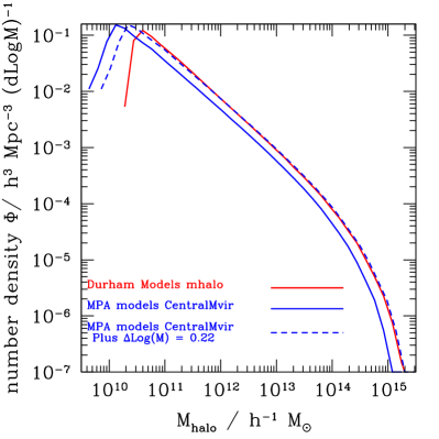
The differences in these definitions of halo mass are apparent in Fig. 1, in which we plot the mass function of dark matter haloes using the Durham and Munich halo mass “labels”. It is immediately clear from this plot that the halo mass labels used by each group do not correspond to a simple particle number returned by a percolation group finder. The absence of a sharp cut-off in the Munich mass function corresponding to the 20 particle limit imposed on the list of FOF groups stored is due to how the virial mass is estimated from the number of particles that the group finder says belong to each halo.
At the present day the mass functions can be brought into remarkably close agreement with one another by rescaling the mass in one of the models by a constant factor. We apply this scaling to the Munich masses so that afterwards, haloes with the same abundance have the same mass444We note that a similar scaling can be performed to match the halo mass functions at different redshifts. However, the scaling does not work quite so well as it does at , and the factor required changes with redshift.. We need to make this rescaling as we plot many of our comparisons as a function of halo mass.
3.2 Galaxy properties
| Density cut 1 | Density cut 2 | Density cut 3 | |||||||
|---|---|---|---|---|---|---|---|---|---|
| Abundance | Mpc-3 | Mpc-3 | Mpc-3 | ||||||
| Model | |||||||||
| Bower et al., 2006 | |||||||||
| Font et al., 2008 | |||||||||
| De Lucia et al., 2007 | |||||||||
| Guo et al., 2011 | |||||||||
| Bertone et al., 2007 | |||||||||
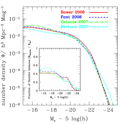
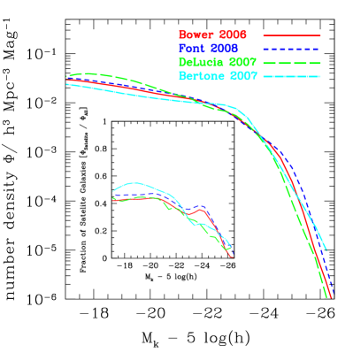
The luminosity function is the most basic description of the galaxy population. As such, reproducing this statistic is a primary goal when setting the parameters of a galaxy formation model.
The present day luminosity functions in the and bands predicted by the models are plotted in Fig. 2. Note that we have added to the magnitudes stored in the Millennium Archive for the Munich models to put them onto the same scale as the Durham models. The agreement between the model predictions is encouraging. To some extent, the model parameters have been selected to reproduce the observed luminosity function, and so one might expect the predictions to agree even better. The models were not necessarily tuned to explicitly match the luminosity functions in these particular bands. The later versions of the Munich models put more emphasis on matching the inferred stellar mass function. Furthermore, other observables are matched at the same time as reproducing the luminosity function data, which may have led to compromises in the quality of the reproduction of the luminosity function. Finally, the parameter values were set by doing comparisons “by eye” between the model predictions and the data. It is not currently possible to provide a definitive list of precisely which datasets were used by the various authors to set the model parameters, or to specify the priorities assigned to the reproduction of different datasets. This should become more transparent with future releases of the models, following the development of statistical approaches to quantify goodness of fit and the weighting of datasets in the parameter setting process (Henriques et al. 2009; Bower et al. 2010; Henriques et al. 2012).
The inset panels in Fig. 2 show the fraction of galaxies that are satellites of the central galaxy within each halo as a function of magnitude. Again the models show similar trends, with just under half of the galaxies being satellites over most of the magnitude range plotted, before this value drops steadily brightwards of . Satellites and centrals are described separately in halo occupation distributions, so this will have implications later on.
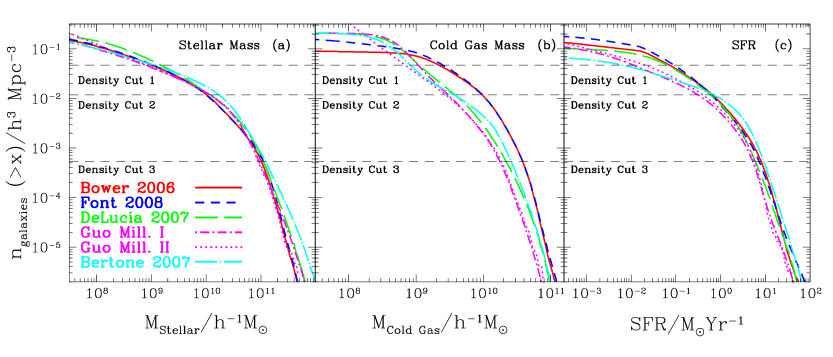
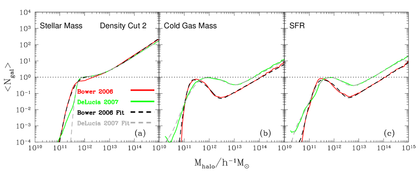
When we study the clustering predicted by the models, we will use samples defined by intrinsic properties: stellar mass, cold gas mass and star formation rate. The cumulative abundance of galaxies ranked by each of these properties in turn is shown in Fig. 3. There is remarkably close agreement between the distributions ranked in terms of stellar mass (left panel of Fig. 3), which is surprising given the differences in the choice of stellar initial mass function in the models, which means that for a given mass of stars made, different amounts of light will be produced, and at least some of the models have been specified to reproduce observed luminosity functions.
The model predictions agree less well when galaxies are ranked in terms of cold gas. The Durham models predict more galaxies for cold gas masses in excess of . This can be traced to less weight being given to fitting the observed gas fractions in spiral galaxies in the Bower2006 and Font2008 models. We note that the new treatment of star formation in the Durham models introduced by Lagos et al. (2011a, b), which distinguishes between atomic and molecular hydrogen in the interstellar medium, gives an excellent match to the observed HI mass function555This model is not included in this paper because, at the time of writing, it was not available in the Millennium Simulation database. The model will be added early in 2013.. The distributions ranked by SFR are more similar to one another than those for cold gas, presumably because in all cases weight was given to matching the observed optical colour distributions of galaxies.
| Model | Stellar | Cold Gas | SFR |
|---|---|---|---|
| mass | mass | ||
| Density Cut 2 | |||
| Bower2006 | 40% | 3% | 3% |
| Font2008 | 42% | 8% | 10% |
| DeLucia2007 | 38% | 6% | 8% |
| Bertone2007 | 37% | 9% | 14% |
| Guo2011 | 41% | 24% | 19% |
| Density Cut 3 | |||
| Bower2006 | 27% | 2% | 1% |
| Font2008 | 26% | 6% | 2% |
| DeLucia2007 | 24% | 2% | 4% |
| Bertone2007 | 27% | 3% | 6% |
| Guo2011 | 26% | 15% | 16% |
To ensure we are making a fair comparison between the models, we define our galaxy samples by number density rather than by a fixed value of a property, such as the stellar mass. Hence, to obtain samples which contain the same number of galaxies, slightly different cuts on a particular property are applied to each model. The cuts used on each property and the number densities of the high, intermediate and low density samples are listed in Table 1. This idea of comparing galaxy catalogues at a fixed number density was applied by Berlind et al. (2003) and Zheng et al. (2005) in their HOD analysis of galaxies output by a gas dynamic simulation and a semi-analytical model. In the Berlind et al. study, the galaxy mass functions output by the two galaxy formation models were very different. Nevertheless, by comparing samples as a fixed abundance, these authors were able to find common features in the HODs. The percentage of galaxies that are satellite galaxies is listed in Table 2.
The finite resolution of the Millennium simulation means that the model predictions are incomplete below some number density. To investigate this we plot the results for the Guo et al. model obtained from the Millennium II simulation (Boylan-Kolchin et al. 2008), which has a halo mass resolution that is 125 times better than that of the Millennium-I run. The comparison between the galaxy catalogues from the Millennium-I and Millennium-II runs shown in Fig. 3 indicates that the Guo et al. model predictions from Millennium-I are robust for stellar masses and star formation rates down to our highest number density cut. The cumulative distributions agree extremely well from the two simulations for stellar mass. In the case of star formation rate, the shapes of the two distributions agree quite well, but with a small displacement. For cold gas, the distributions are different at low masses. For this reason, we omit comparisons corresponding to the first density cut in the case of cold gas and star formation rate, which to some extent is controlled by the cold gas content. Ideally this exercise should be repeated by comparing the Millennium-I and Millennium-II predictions for each model in turn, as the convergence is likely to be model dependent. However, the Millennium-II outputs are not currently available in the database for each model.
Our methodology of matching the halo mass “labels” between models and of comparing samples with, by construction, exactly the same number of galaxies allows us to focus on differences in the way in which the models populate haloes with galaxies.
3.3 Further adjustments to the halo masses in the Munich model
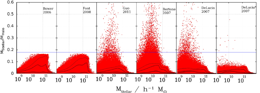
We are almost in a position to compare HODs between models. Before we do this, we first carry out a preliminary investigation of how galaxy properties correlate with halo mass, by plotting the stellar mass to the host halo mass ratio in Fig. 4. This ratio is formed using the mass of the host halo at the present day which is the relevant mass for HODs (rather than the subhalo mass associated with each galaxy, which is used in subhalo abundance matching e.g. Simha et al. 2012). The median ratios of stellar mass to halo mass are similar between the models, as shown by the solid lines in Fig. 4. The extremes of the distribution and the outliers, are, however, different.
The maximum value of the ratio of stellar mass to host halo mass is the universal baryon fraction, since all of the models assume that dark matter haloes initially have this baryonic mass associated with them. This extreme case corresponds to the presence of a single galaxy in the halo with all of the baryons in the form of stars, with no hot gas or cold gas. The first two panels of Fig. 4 show that the Durham models match this expectation with all of the galaxies lying below the limit indicated by the horizontal blue dotted line. Indeed most galaxies are far away from this line, as indicated by the percentile curves, which reflects how inefficient galaxy formation is at turning baryons into stars (Cole et al. 2001; Baugh 2006).
The Munich models, on the other hand, throw up a small number of galaxies (fewer than 1%) in which the stellar mass appears to exceed the universal baryon fraction, in some cases by a substantial factor, becoming comparable to the host halo mass (in fact in a very small number of cases the galaxy stellar masses even exceeds the associated halo mass). Closer inspection of the merger histories reveals that these galaxies, despite being labelled at the present day as central galaxies, reside in haloes that have been tidally stripped in the past. The halo spent one or more snapshots orbiting within a larger halo during which a substantial amount of mass was lost, leading to artificially high stellar mass to halo mass ratios. This scenario does not happen by construction with the Durham algorithm used to build merger trees (see Merson et al. 2012 and Jiang et al., in preparation). The stripping of mass from halos is a physical effect. However, the extent of the mass stripping will be somewhat dependent on the simulation parameters. This ambiguity over the labelling of halo masses will have an impact on the shape of the predicted HOD, particularly at low halo masses.
To enable a fair comparison between the predictions between the Durham and Munich models, we attempted an approximate correction to the Munich halo masses. By examining the galaxy merger trees, we identified galaxies which, at the present day, are labelled as a central galaxy, but whose host halo was once a satellite halo in a more massive structure. We then trace the more massive host halo to the present day and assign this halo mass to the galaxy instead. The galaxy is relabelled as a satellite and is associated with the more massive halo, resulting in the galaxy moving down and across in Fig. 4. We have performed this postprocessing only in the case of the DeLucia2007 model, which we label as DeLucia2007* in the right-most panel of Fig. 4. This procedure affects of the galaxies in the DeLucia2007 model, altering the tail of the distribution of the stellar mass to halo mass ratio, moving the 99% line (but not the 90% line) and greatly reduces the number of galaxies whose stellar mass exceeds the mass of baryons attached to the associated host halo.
4 Results
The main results of the paper are presented in this section, following the preparatory work on the galaxy samples downloaded from the Millennium Archive, as outlined in the previous section. In Section 4.1, we compare the model predictions for samples defined in terms of stellar mass, looking at the HOD and the two-point correlation function. We examine the contribution to the correlation function from satellite and central galaxies, and compare the radial extent of galaxies in common haloes. A similar study is made for samples ranked by cold gas in Section 4.2 and star formation rate in Section 4.3.
4.1 Stellar mass
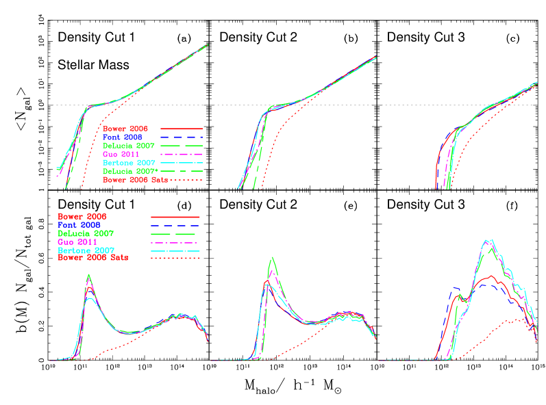
The HODs predicted by the models when galaxies are ranked by their stellar mass are plotted in the top panel of Fig. 5. The agreement between the model predictions for the high density sample is spectacular (left panel of Fig. 5). The Munich models display a slight kink at very low mean numbers of galaxies per halo compared to the Durham models. This is the regime in which only a tiny fraction of haloes, roughly 1 in 1000, contain a galaxy which meets the selection criteria. In the case of DeLucia2007*, where we have applied a further correction to a small fraction of halo masses as described in the previous section, the agreement with the Durham models improves and holds for all masses plotted. Here, a galaxy that was originally a central galaxy in a halo which has been heavily stripped is now treated as a satellite galaxy in a more massive halo.
The predicted HODs are qualitatively similar for the intermediate and low density samples (middle and right panels of Fig. 5). However, in detail the HODs are different, particularly around the halo masses at which central galaxies first start to make it into the samples. Note that in the lowest density sample (corresponding to the most massive galaxies), there is no extended plateau feature corresponding to the situation in which all haloes contain a central galaxy that is included in the sample. There is a knee in the HOD around a halo mass of , corresponding to the halo mass at which one in ten haloes contains a central galaxy which is sufficiently massive to be included in the sample. Satellite galaxies make an appreciable contribution to the HOD long before the mean number of galaxies per halo reaches unity, showing that the canonical HOD model of a step function for centrals which reaches unity, plus a power law for satellites, is a poor description of the model predictions.
The variation in the form of the predicted HOD for different number densities can be explained in terms of the relative importance of AGN feedback which suppresses gas cooling in massive haloes. The highest number density sample (ie. corresponding to the lowest stellar mass cuts in each model) is dominated by galaxies in haloes which are not affected by AGN feedback, since a mean galaxy occupation of unity is reached for haloes of mass .
For the lower density samples (higher stellar masses), the form of the HOD is sensitive to the operation of AGN/radio mode feedback. The suppression of cooling in massive haloes changes the slope and scatter of the stellar mass - halo mass relation (Gonzalez-Perez et al. 2011). With this feedback mode, the most massive galaxies are not necessarily in the most massive haloes. This is particularly true in the case of the Durham models, which show more scatter between stellar mass and halo mass than is displayed by the Munich models (Contreras et al. in prep.). The consumption of cold gas in a starburst when a disk becomes dynamically unstable may also play a role in determining the form of the HOD for cold gas selected samples. Unstable disks are more common in the Durham models than in the Munich models (Parry et al. 2009).
Differences in the HOD curves can seem quite dramatic, particularly at low masses where the HOD makes the transition from zero galaxies per halo, and at high halo masses, where the HOD is in general a power law. However, the HOD does not give the full view of galaxy clustering. It is important to bear in mind that the number density of dark matter haloes and the clustering bias associated with haloes of a given mass also contribute and these quantities change significantly across the mass range plotted in Fig. 5. Following Kim et al. (2009), we show in the bottom panel of Fig. 5 the contribution to the effective bias of the galaxy sample as a function of halo mass, which takes into account the halo mass function and the halo bias. Note that the y-axis in the bottom panels is on a linear scale. The high and intermediate density samples show two distinct peaks in the contribution to the effective bias, with the low mass peak corresponding to central galaxies and the high mass peak to satellite galaxies. For the low density sample (bottom right panel of Fig. 5), the central galaxy peak is much less distinct and satellite galaxies dominate the effective bias.
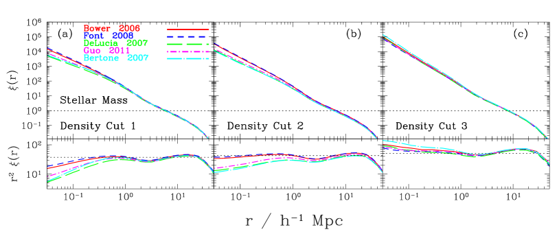
The two-point correlation function of the stellar mass selected samples is plotted in Fig. 6. At larger pair separations (), the correlation functions predicted by the models are remarkably similar, as expected from the similarity in the effective bias plotted in Fig. 5. The variation in the predicted bias, averaged over pair separations of Mpc is less than 10%. At small pair separations, for the lowest density sample, the correlation functions differ by 10-30%. In the case of the intermediate and high density samples, the extremes of the predictions vary by a factor of 2-3, with more clustering predicted in the Durham models than in the Munich models.
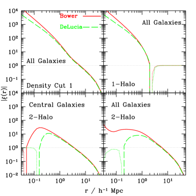
To gain further insight into the correlation functions predicted by the models, we examine the contributions from galaxy pairs in the same halo (the 1-halo term in HOD terminology) and from different halos (the 2-halo term) in Fig. 7, in which we compare the Bower2006 and DeLucia2007 results. The top-left panel confirms that the correlation functions are remarkably close to one another, except for pair separations smaller than Mpc. This difference is dominated by the 1-halo term (top-right panel), which itself is largely determined by satellite-satellite pairs. In the Bower2006 model the 2-halo term makes a small contribution to the amplitude of the correlation function at these pair separations, whereas in the DeLucia2007, centrals contribute no pairs at these scales. This difference can be understood in terms of the DHalos algorithm used to build halo merger histories, which breaks up some FOF haloes into separate objects, allowing centrals to be found closer together than in the Munich models.
After rescaling the halo masses and considering samples with the same number density of galaxies, we find that the Bower2006 and DeLucia2007 models contain very similar numbers of satellite galaxies per halo, as revealed by the close agreement between the HODs plotted in Fig. 5 (see Table 2). This implies that overall, the timescale for galaxies to merge must be similar in the models. Both models use analytical calculations of the time required for a satellite to merge with the central galaxy, based on the dynamical friction timescale (see Lacey & Cole (1993); Cole et al. (2000)). Very similar expressions are used for this timescale, with an adjustable parameter chosen to extend the timescales in both cases to improve the model predictions for the bright end of the galaxy luminosity function. In the Munich models, the satellite orbit is followed as long as the associated subhalo can be resolved, then the time required for the satellite to merge with the central is calculated analytically. In the Durham models, the merger timescale is calculated as soon as the galaxy becomes a satellite, without any consideration as to whether or not the associated subhalo can still be identified.
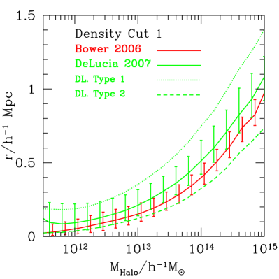
The reason for the enhanced small scale clustering in the Durham model must therefore be due to a difference in the spatial distribution of these satellites within dark matter haloes. Fig. 8 confirms this, showing the median separation between the central galaxy in a halo and its satellites. The median satellite radius is greater in the Munich model than in the Durham model. This is readily understood from the way in which the merger times are calculated. In the Munich model, satellite galaxies whose subhaloes can be resolved do not merge with the central galaxy. In the Durham model, some fraction of galaxies which are associated with an identifiable subhalo will be assumed to have merged, as a result of the purely analytical calculation of the merger time. The spatial distribution of satellites with resolved subhaloes is more extended than the overall distribution of satellites. This is clear from Fig. 8 which shows that Type 1 satellites in the DeLucia2007 model, i.e. those with resolved subhaloes, have a larger median radius than satellites whose subhalo can no longer be identified (Type 2 satellites). There are around three times as many satellites with resolved subhaloes in the DeLucia model compared with the Bower model.
4.2 Cold gas mass
The models considered in this paper track the total mass in cold gas, combining helium and hydrogen, the latter in both its atomic and molecular forms. All of this material is assumed to be available to make stars. With each episode of star formation, some cold gas will be ejected from the ISM and perhaps from the dark matter halo altogether due to supernovae. More recent models make the distinction between molecular and atomic hydrogen using the pressure in the mid-plane of the galactic disk and assume that only the molecular hydrogen is involved in star formation (see for example Lagos et al. 2011b).
The comparison presented in Fig. 3 between the cumulative cold gas mass function predicted in the Guo et al. model in the Millennium-I and Millennium-II simulations suggests that the predictions have not converged for the highest density sample, corresponding to the lowest cut in cold gas mass. Hence we compare the predicted HODs only for the two lower density cuts in Fig. 9, which correspond to higher cold gas masses. There is a range of HOD predictions.
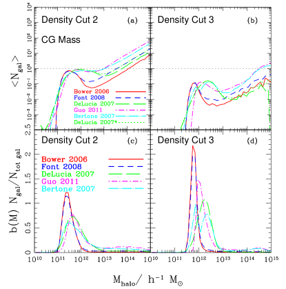
The predicted HOD for central galaxies tends to show a peak rather than a step. This feature is particularly clear in the lowest density sample. This form of the HOD is due to the inclusion of AGN feedback in the models, which suppresses gas cooling in massive haloes (see the plot of cold gas mass versus halo mass in Kim et al. 2011). In the Munich models, the suppression of cooling comes in gradually (Croton et al. 2006), whereas in the Durham models, the suppression is total in haloes in which the AGN feedback is operative (Bower et al. 2006). We present a parametric fit to the form of the HOD of samples selected by cold gas mass in the Appendix, in which we advocate using the nine parameter fit of Geach et al. (2012) to describe the HOD predicted by the models.
Satellites make up a smaller fraction of samples selected by cold gas mass (see Table 2). The satellite HOD is a power-law as it was in the case of samples selected according to their stellar mass, but with a shallower slope (). There is a substantial range in the amplitude of the satellite HODs, which differ by a factor of 5 between the extremes. This is consistent with the variation in the percentage of galaxies in each sample that are satellites, as listed in Table 2. This is due in part to the way in which the model parameters were set. The Bower2006 and Font2008 models overpredict the observed cold gas mass function (Kim et al. 2011). The Font2008 model invokes a revised model for gas cooling in satellites, in which the hot gas attached to the satellite is only partially stripped, with the fraction of material removed depending upon the orbit of the satellite. Hence, gas can still cool onto satellites in the Font et al. model, which explains why the satellite HOD is higher in this model than in Bower et al666We note that the latest version of the Munich model (Guo et al. 2011) includes a similar treatment of gas cooling onto satellites to that introduced by Font et al. However, these authors do not present a plot showing how the model predictions compare with cold gas data, so we cannot comment on the difference between the Guo2011 and Durham models for the cold gas mass function..
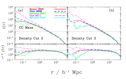
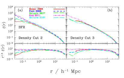
The lower panels of Fig. 9 show that central galaxies dominate the contribution to the bias factor for cold gas selected samples. The peak in these contributions covers a factor of in halo mass for the intermediate density sample and an order of magnitude for the low density sample. This lack of consensus between the model predictions is borne out in the predicted correlation functions of cold gas selected samples plotted in Fig. 10. On the whole, the correlation function for cold gas samples is shallower than that for stellar mass samples, with a slope around rather than , due to the less important role of satellite galaxies in the cold gas samples. There is a spread of a factor of in the clustering amplitude around Mpc and of around an order of magnitude or more at the smallest pair separations plotted.
4.3 Star formation rate
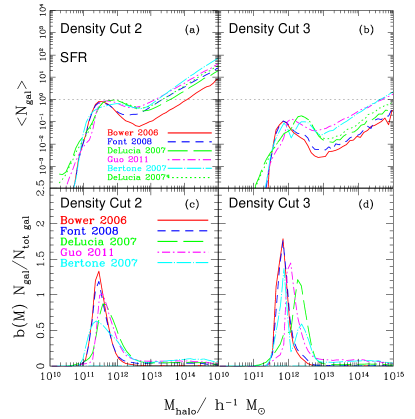
Finally, we repeat the analysis of the previous section using samples ranked by the global star formation rate in the galaxy, which is relevant to observational samples selected by emission line strength or rest-frame UV luminosity. The predicted HODs plotted in Fig. 11 are very similar to those for the cold gas samples plotted in Fig. 9. In the Bower2006 and Font2008 models there is a direct connection between the total cold gas mass and the star formation rate. In the Munich models, only the gas above a surface density threshold is assumed to participate in star formation. The correlation functions plotted in Fig. 12 also show a shallower slope than those obtained for the stellar mass selected samples. The predicted clustering shows a similar spread to that displayed for cold gas selected samples.
5 Conclusions
We have tested the robustness of the predictions of semi-analytical models of galaxy formation for the clustering of galaxies. This project was made possible through the Millennium Simulation database, which allows the outputs of the models to be downloaded and analyzed by the astronomical community.
The models tested were produced by the “Durham” and “Munich” groups, and represent different versions of their “best bet” models when originally published. These codes attempt to model the fate of the baryonic component of the universe. The underlying physics is complex and still poorly understood despite much progress over the past twenty years. Although the two groups developed their approaches starting from White & Frenk (1991), the implementations of the different processes which influence galaxy formation are quite different, as is the emphasis on which observations should be reproduced by the models in order to set the values of the model parameters. The calculations are set in the Millennium N-body simulation of Springel et al. (2005). However, all aspects of galaxy formation modelling beyond the distribution of the dark matter, including the construction of merger histories for halos, are independent.
Given the uncertainty in the modelling of galaxy formation, the availability of model outputs from the same N-body simulation gives us an opportunity to perform a direct comparison of how the models populate halos with galaxies. We have carried out this comparison by looking at the model predictions for the halo occupation distribution (which it should be stressed is a model output) and the two-point correlation function. We compare samples at fixed abundances, high, medium and low, to account for any differences in the distributions of galaxy properties which persist between the model predictions. We also use a common definition of halo mass, again by referring to the abundance of haloes. We look at samples defined by intrinsic properties: stellar mass, cold gas mass and star formation rate.
In the case of samples selected by their stellar mass, the agreement in the predicted HODs is remarkable, particularly as galaxy clustering is in general not one of the observables used to specify the model parameters. The two-halo contributions to the correlation function are the same in different models, which means that, under the conditions of the controlled comparison carried out here, the prediction for the asymptotic galaxy bias is robust.
The one-halo term, i.e. the contribution from pairs in the same dark matter halo, is different. Again, under the conditions of our comparison, there is little difference in the number of satellite galaxies in each halo which implies that the calculation of the timescale required for a galaxy merger to take place is similar in the two sets of models. The difference lies in which galaxies are considered for mergers. In the Durham models, any satellite can merge provided that the dynamical friction timescale is sufficiently short for the merger to have time to take place. In the Munich models, only those satellites which are hosted by subhaloes which can no longer be identified can merge. The radial distribution of subhaloes is more extended than the distribution of dark matter (Angulo et al. 2009), so this naturally leads to larger 1-halo pair separations in the Munich models. It is fair to argue that here the Munich approach is more reasonable, though this depends on how well the subhalo finder works.
Budzynski et al. (2012) compared the radial density profile of galaxies in clusters using a subset of the semi-analytical models considered here, and argued that, for their selection, the Durham models produced longer merger timescales for satellites than in the Munich models, to explain a steeper inner profile. Our conclusion is different, as we argue that the merger timescales are similar but that the effective radial distribution of galaxies is different. This difference in interpretation could be due, however, to the way in which galaxy samples are compiled in both studies.
The agreement between the models is less good when looking at samples selected by cold gas mass and star formation rate. In these cases the models give qualitatively similar predictions which differ in detail. There is a small spread in the asymptotic bias (a factor of ) and a large difference (order of magnitude) in the small scale correlation function. One notable difference from the samples selected by stellar mass is the form of the HOD predicted for cold gas and star formation rate samples. In the latter two cases the HOD for central galaxies has an asymmetrical peak, rather than the worn step function seen for stellar mass samples.
The conclusion of our study is that for some galaxy properties, different models of galaxy formation give encouragingly similar predictions for galaxy clustering. This means that there is some hope of understanding galaxy bias in terms of the implications for galaxy formation physics, and from the point of view of removing it as a systematic in dark energy probes. However, this depends on the sample selection, and for surveys which target emission lines, the current predictions agree less well. Also, the absolute value of the bias predicted by the models may differ if an observational selection is applied to the catalogues, as would be done in a mock catalogue, rather than performing the controlled test we carried out of comparing samples at a fixed number density. It is also important to bear in mind that we have tested how closely the models predict galaxy bias in a single cosmology. In reality, we do not know the true underlying cosmology in the real Universe, and this will further complicate the attempt to extract the underlying clustering of the mass. As the modelling of the gas content and star formation rate in galaxies improves (Lagos et al. 2011b), hopefully the predictions for samples selected by e.g. emission line properties will become more robust.
Acknowledgements
This work would have been much more difficult without the efforts of Gerard Lemson and colleagues at the German Astronomical Virtual Observatory in setting up the Millennium Simulation database in Garching, and John Helly and Lydia Heck in setting up the mirror at Durham. We acknowledge helpful conversations with the participants in the GALFORM lunches in Durham. This work was partially supported by “Centro de Astronomía y Tecnologías Afines” BASAL PFB-06. NP was supported by Fondecyt Regular #1110328. We acknowledge support from the European Commission’s Framework Programme 7, through the Marie Curie International Research Staff Exchange Scheme LACEGAL (PIRSES-GA-2010-269264). PN acknowledges the support of the Royal Society through the award of a University Research Fellowship and the European Research Council, through receipt of a Starting Grant (DEGAS-259586). The calculations for this paper were performed on the ICC Cosmology Machine, which is part of the DiRAC-2 Facility jointly funded by STFC, the Large Facilities Capital Fund of BIS, and Durham University and on the Geryon cluster at the Centro de Astro-Ingenieria at Universidad Católica de Chile.
References
- Angulo et al. (2009) Angulo R. E., Lacey C. G., Baugh C. M., Frenk C. S., 2009, MNRAS, 399, 983
- Balogh et al. (2001) Balogh M. L., Pearce F. R., Bower R. G., Kay S. T., 2001, MNRAS, 326, 1228
- Baugh (2006) Baugh C. M., 2006, Reports on Progress in Physics, 69, 3101
- Benson (2010) Benson A. J., 2010, PhysRep, 495, 33
- Benson et al. (2003) Benson A. J., Bower R. G., Frenk C. S., Lacey C. G., Baugh C. M., Cole S., 2003, ApJ, 599, 38
- Berlind et al. (2003) Berlind A. A. et al., 2003, ApJ, 593, 1
- Bertone et al. (2007) Bertone S., De Lucia G., Thomas P. A., 2007, MNRAS, 379, 1143
- Bower et al. (2006) Bower R. G., Benson A. J., Malbon R., Helly J. C., Frenk C. S., Baugh C. M., Cole S., Lacey C. G., 2006, MNRAS, 370, 645
- Bower et al. (2010) Bower R. G., Vernon I., Goldstein M., Benson A. J., Lacey C. G., Baugh C. M., Cole S., Frenk C. S., 2010, MNRAS, 407, 2017
- Boylan-Kolchin et al. (2008) Boylan-Kolchin M., Ma C.-P., Quataert E., 2008, MNRAS, 383, 93
- Budzynski et al. (2012) Budzynski J. M., Koposov S. E., McCarthy I. G., McGee S. L., Belokurov V., 2012, MNRAS, 423, 104
- Cole et al. (2000) Cole S., Lacey C. G., Baugh C. M., Frenk C. S., 2000, MNRAS, 319, 168
- Cole et al. (2001) Cole S. et al., 2001, MNRAS, 326, 255
- Cooray & Sheth (2002) Cooray A., Sheth R., 2002, PhysRep, 372, 1
- Croton et al. (2006) Croton D. J. et al., 2006, MNRAS, 365, 11
- De Lucia & Blaizot (2007) De Lucia G., Blaizot J., 2007, MNRAS, 375, 2
- De Lucia et al. (2004) De Lucia G., Kauffmann G., White S. D. M., 2004, MNRAS, 349, 1101
- De Lucia et al. (2006) De Lucia G., Springel V., White S. D. M., Croton D., Kauffmann G., 2006, MNRAS, 366, 499
- Font et al. (2008) Font A. S. et al., 2008, MNRAS, 289, 1619
- Geach et al. (2012) Geach J. E., Sobral D., Hickox R. C., Wake D. A., Smail I., Best P. N., Baugh C. M., Stott J. P., 2012, MNRAS, 426, 679
- Gonzalez-Perez et al. (2011) Gonzalez-Perez V., Baugh C. M., Lacey C. G., Kim J.-W., 2011, MNRAS, 417, 517
- Guo et al. (2011) Guo Q. et al., 2011, MNRAS, 413, 101
- Henriques et al. (2012) Henriques B., White S., Thomas P., Angulo R., Guo Q., Lemson G., Springel V., 2012, ArXiv e-prints, arXiv1212.1717
- Henriques et al. (2009) Henriques B. M. B., Thomas P. A., Oliver S., Roseboom I., 2009, MNRAS, 396, 535
- Kim et al. (2011) Kim H.-S., Baugh C. M., Benson A. J., Cole S., Frenk C. S., Lacey C. G., Power C., Schneider M., 2011, MNRAS, 414, 2367
- Kim et al. (2009) Kim H.-S., Baugh C. M., Cole S., Frenk C. S., Benson A. J., 2009, MNRAS, 400, 1527
- Lacey & Cole (1993) Lacey C., Cole S., 1993, MNRAS, 262, 627
- Lagos et al. (2011a) Lagos C. D. P., Baugh C. M., Lacey C. G., Benson A. J., Kim H.-S., Power C., 2011a, MNRAS, 418, 1649
- Lagos et al. (2011b) Lagos C. D. P., Lacey C. G., Baugh C. M., Bower R. G., Benson A. J., 2011b, MNRAS, 416, 1566
- Laureijs et al. (2011) Laureijs R. et al., 2011, ArXiv e-prints, arXiv1110.3193
- McCarthy et al. (2007) McCarthy I. G., Bower R. G., Balogh M. L., 2007, MNRAS, 377, 1457
- Merson et al. (2012) Merson A. I. et al., 2012, MNRAS, 342
- Parry et al. (2009) Parry O. H., Eke V. R., Frenk C. S., 2009, MNRAS, 396, 1972
- Schlegel et al. (2011) Schlegel D. et al., 2011, ArXiv e-prints, arXiv1106.1706
- Simha et al. (2012) Simha V., Weinberg D. H., Davé R., Fardal M., Katz N., Oppenheimer B. D., 2012, MNRAS, 423, 3458
- Springel et al. (2005) Springel V. et al., 2005, Nature, 435, 629
- Springel et al. (2001) Springel V., White S. D. M., Tormen G., Kauffmann G., 2001, MNRAS, 328, 726
- White & Frenk (1991) White S. D. M., Frenk C. S., 1991, ApJ, 379, 52
- Zehavi et al. (2005) Zehavi I. et al., 2005, ApJ, 630, 1
- Zheng et al. (2005) Zheng Z. et al., 2005, ApJ, 633, 791
Appendix A Parametric fits to the HODs predicted by the semi-analytical models
| Model | |||||
|---|---|---|---|---|---|
| Bower2006 | |||||
| DeLucia2007 |
| Model | |||||||||
|---|---|---|---|---|---|---|---|---|---|
| Cold Gas Mass | |||||||||
| Bower2006 | |||||||||
| DeLucia2007 | |||||||||
| SFR | |||||||||
| Bower2006 | |||||||||
| DeLucia2007 |
Semi-analytical galaxy formation models follow the processes which influence the baryonic component of the Universe, in order to predict the number of galaxies hosted by dark matter haloes along with the properties of the galaxies. The HOD is therefore a natural prediction of semi-analytical models. In this appendix, we compare the HODs output by the semi-analytical models with examples of the parametric forms typically used in the HOD analyses of galaxy clustering. Note that we fit the parametric form directly to the HOD output by the model and not to the HOD predictions for the correlation function and galaxy abundance, as is done when comparing HOD models to observations (Cooray & Sheth 2002; Zehavi et al. 2005).
As we remarked in the paper, the form of the HOD predicted by the models is sensitive to the manner in which galaxies are selected. Following the standard practice with HOD fitting, we can separate the model output into contributions from central galaxies and satellites. The largest variations in the model predictions are seen in the HOD of central galaxies when different selections are applied. The central HOD for samples defined by stellar mass is almost a step function, but with a more gradual transition from a mean occupation of zero galaxies per halo to one galaxy per halo. For samples corresponding to high stellar mass galaxies, the predicted central galaxy HOD need not reach unity, even for the most massive haloes. In the case of samples constructed on the basis of star formation rate or cold gas mass, the central HOD is peaked rather than a step. Such a feature would be hard to anticipate but can be readily understood in terms of the physics in the semi-analytical models. The HOD of satellite galaxies is approximately a power law and varies mainly in normalization between different selections.
The first parametrization of the HOD we consider is the five parameter form proposed by Zheng et al. (2005). The HOD is broken up into the contributions from the mean number of satellite galaxies and centrals (i.e. the fraction of halos of a given mass which contain a central galaxy passing the selection if ) per halo, with the overall mean number of galaxies per halo given by . The central galaxy HOD is a rounded step function, with a gradual transition from zero to one central galaxy per halo on average:
| (1) |
Here is the mass of the host dark matter halo, the error function,
| (2) |
is the mass at which the half of the halos have at least one galaxy and is the width in halo mass of the transition from zero to one galaxy per halo. The HOD for satellite galaxies is given by
| (3) |
where is the mass below which a halo can not host a satellite galaxy and is the mass in which a halo contains on average 1 satellite galaxy and is the power-law slope, which usually has a value close to unity.
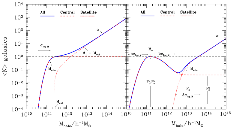
A schematic of the 5-parameter HOD with an explanation of which features the parameters control is given in the left-hand panel of Fig. A1. The best fitting values of the parameters of this HOD model are listed in Table A1 for the intermediate abundance stellar mass selected samples from the Bower2006 and DeLucia2007 models. The predicted HODs and the fits are plotted in Fig. A2.
In the case of samples selected by cold gas mass or SFR, the form of the predicted HOD is very different from that for stellar mass selected samples. The HOD of central galaxies is peaked, as noted by Kim et al. (2011). The five parameter HOD cannot describe this behaviour. Instead, the nine parameter fit advocated by Geach et al. (2012) is more appropriate, with one modification. In this case, the central HOD is now given by
| (4) | |||
where are normalization factors (with values varying between zero and one), is the central value of the Gaussian. The modification we have made is to allow the width of the Gaussian to be different for masses on either side of . The dispersion is for halos with mass and for those with . This allows the best fitting central HOD to be an asymmetric peak. The satellite HOD is given by:
| (5) |
where is the mean number of satellites per halo halo at the “transition” mass , which corresponds roughly to the mass above which the mean number of galaxies per halo is dominated by satellites, represents the width of the transition from zero satellites per halo to the power law, and is the slope of the power-law which gives the mean number of satellites for
A schematic of the 9-parameter HOD, along with an explanation of which features the parameters control is given in the right-hand panel of Fig. A1. The best fitting values of the parameters of this HOD model are listed in Table A2 for the intermediate abundance cold gas mass and star formation rate selected samples from the Bower2006 and DeLucia2007 models. The predicted HODs and the fits are plotted in Fig. A2.