Boltzmann Machines and Denoising Autoencoders
for Image Denoising

KyungHyun Cho
Aalto University School of Science
Department of Information and Computer Science
Espoo, Finland
kyunghyun.cho@aalto.fi

Abstract

Image denoising based on a probabilistic model of local image patches has been employed by various researchers, and recently a deep (denoising) autoencoder has been proposed by Burger et al. (2012) and Xie et al. (2012) as a good model for this. In this paper, we propose that another popular family of models in the field of deep learning, called Boltzmann machines, can perform image denoising as well as, or in certain cases of high level of noise, better than denoising autoencoders. We empirically evaluate the two models on three different sets of images with different types and levels of noise. Throughout the experiments we also examine the effect of the depth of the models. The experiments confirmed our claim and revealed that the performance can be improved by adding more hidden layers, especially when the level of noise is high.

1 Introduction

Numerous approaches based on machine learning have been proposed for image denoising tasks over time. A dominant approach has been to perform denoising based on local statistics over a whole image. For instance, a method denoises each small image patch extracted from a whole noisy image and reconstructs the clean image from the denoised patches. Under this approach, it is possible to use raw pixels of each image patch (see, e.g. Hyvärinen et al., 1999) or the representations in another domain, for instance, in wavelet domain (see, e.g. Portilla et al., 2003).

In the case of using raw pixels, sparse coding has been a method of choice. Hyvärinen et al. (1999) proposed to use independent component analysis (ICA) to estimate a dictionary of sparse elements and compute the sparse code of image patches. Subsequently, a shrinkage nonlinear function is applied to the estimated sparse code elements to suppress those elements with small absolute magnitude. This sparse code elements are used to reconstruct a noise-free image patch. More recently, Elad and Aharon (2006) also showed that sparse overcomplete representation is useful in denoising images. Some researchers claimed that better denoising performance can be achieved by using a variant of sparse coding methods (see, e.g. Shang and Huang, 2005; Lu et al., 2011).

In essence, these approaches build a probabilistic model of natural image patches using a layer of sparse latent variables. The posterior distribution of each noisy patch is either exactly computed or estimated, and the noise-free patch is reconstructed as an expectation of a conditional distribution over the posterior distribution.

Based on this interpretation, some researchers have proposed very recently to utilize a (probabilistic) model that has more than one layers of latent variables for image denoising. Burger et al. (2012) showed that a deep multi-layer perceptron that learns a mapping from a noisy image patch to its corresponding clean version, can perform as good as the state-of-the-art denoising methods. Similarly, Xie et al. (2012) proposed a variant of a stacked denoising autoencoder (Vincent et al., 2010) that is more effective in image denoising. They were also able to show that the denoising approach based on deep neural networks performed as good as, or sometimes better than, the conventional state-of-the-art methods.

Along this line of research, we aim to propose a yet another type of deep neural networks for image denoising, in this paper. A Gaussian-Bernoulli restricted Boltzmann machines (GRBM) (Hinton and Salakhutdinov, 2006) and deep Boltzmann machines (GDBM) (Salakhutdinov and Hinton, 2009; Cho et al., 2011b) are empirically shown to perform well in image denoising, compared to stacked denoising autoencoders. Furthermore, we extensively evaluate the effect of the number of hidden layers of both Boltzmann machine-based deep models and autoencoder-based ones. The empirical evaluation is conducted using different noise types and levels on three different sets of images.

2 Deep Neural Networks

We start by briefly describing Boltzmann machines and denoising autoencoders which have become increasingly popular in the field of machine learning.

2.1 Boltzmann Machines

Originally proposed in 1980s, a Boltzmann machine (BM) (Ackley et al., 1985) and especially its structural constrained version, a restricted Boltzmann machine (RBM) (Smolensky, 1986) have become increasingly important in machine learning since (Hinton and Salakhutdinov, 2006) showed that a powerful deep neural network can be trained easily by stacking RBMs on top of each other. More recently, another variant of a BM, called a deep Boltzmann machine (DBM), has been proposed and shown to outperform other conventional machine learning methods in many tasks (see, e.g. Salakhutdinov and Hinton, 2009).

We first describe a Gaussian-Bernoulli DBM (GDBM) that has $L$ layers of binary hidden units and a single layer of Gaussian visible units. A GDBM is defined by its energy function

	$\displaystyle-E$	$\displaystyle(\mathbf{v},\mathbf{h}\mid{\boldsymbol{\theta}})=\sum_{i}-\frac{(v_{i}-b_{i})^{2}}{2\sigma^{2}}+\sum_{i,j}\frac{v_{i}}{\sigma^{2}}h_{j}^{(1)}w_{i,j}+\sum_{j}h_{j}^{(1)}c_{j}^{(1)}+$
		$\displaystyle\sum_{l=2}^{L}\left(\sum_{j}h_{j}^{(l)}c_{j}^{(l)}+\sum_{j,k}h_{j}^{(l)}h_{k}^{(l+1)}u_{j,k}^{(l)}\right),$		(1)

where $\mathbf{v}=\left[v_{i}\right]_{i=1\dots N_{v}}$ and $\mathbf{h}^{(l)}=\left[h_{j}^{(l)}\right]_{j=1\dots N_{l}}$ are $N_{v}$ Gaussian visible units and $N_{l}$ binary hidden units in the $l$ -th hidden layer. $\mathbf{W}=\left[w_{i,j}\right]$ is the set of weights between the visible neurons and the first layer hidden neurons, while $\mathbf{U}^{(l)}=\left[u_{j,k}^{(l)}\right]$ is the set of weights between the $l$ -th and $l+1$ -th hidden neurons. $\sigma^{2}$ is the shared variance of the conditional distribution of $v_{i}$ given the hidden units.

With the energy function, a GDBM can assign a probability to each state vector $\mathbf{x}=[\mathbf{v};\mathbf{h}^{(1)};\cdots;\mathbf{h}^{(L)}]$ using a Boltzmann distribution:

\displaystyle p(\mathbf{x}\mid{\boldsymbol{\theta}})=\frac{1}{Z({\boldsymbol{\theta}})}\exp\left\{-E(\mathbf{x}\mid{\boldsymbol{\theta}})\right\}.

Based on this property the parameters can be learned by maximizing the log-likelihood $\mathcal{L}=\sum_{n=1}^{N}\log\sum_{\mathbf{h}}p(\mathbf{v}^{(n)},\mathbf{h}\mid{\boldsymbol{\theta}})$ given $N$ training samples $\{\mathbf{v}^{(n)}\}_{n=1,\dots,N}$ , where $\mathbf{h}=\left[\mathbf{h}^{(1)};\cdots;\mathbf{h}^{(L)}\right]$ .

Although the update rules based on the gradients of the log-likelihood function are well defined, it is intractable to exactly compute them. Hence, an approach that uses variational approximation together with Markov chain Monte Carlo (MCMC) sampling was proposed by Salakhutdinov and Hinton (2009).

It has, however, been found that training a GDBM using this approach starting from randomly initialized parameters is not trivial (Salakhutdinov and Hinton, 2009; Desjardins et al., 2012; Cho et al., 2012). Hence, Salakhutdinov and Hinton (2009) and Cho et al. (2012) proposed pretraining algorithms that can initialize the parameters of DBMs. In this paper, we use the pretraining algorithm proposed by Cho et al. (2012).

A Gaussian-Bernoulli RBM (GRBM) is a special case of a GDBM, where the number of hidden layers is restricted to one, $L=1$ . Due to this restriction it is possible to compute the posterior distribution over the hidden units conditioned on the visible units exactly and tractably. The conditional probability of each hidden unit $h_{j}=h_{j}^{(1)}$ is

\displaystyle p(h_{j}=1\mid\mathbf{v},{\boldsymbol{\theta}})=f\left(\sum_{i}w_{ij}\frac{v_{i}}{\sigma^{2}}+c_{j}\right).

(2)

Hence, the positive part of the gradient, that needs to be approximated with variational approach in the case of GDBMs, can be computed exactly and efficiently. Only the negative part, which is computed over the model distribution, still relies on MCMC sampling, or more approximate methods such as contrastive divergence (CD) (Hinton, 2002).

2.2 Denoising Autoencoders

A denoising autoencoder (DAE) is a special form of multi-layer perceptron network with $2L-1$ hidden layers and $L-1$ sets of tied weights. A DAE tries to learn a network that reconstructs an input vector optimally by minimizing the following cost function:

\displaystyle\sum_{n=1}^{N}\left\|\mathbf{W}g^{(1)}\circ\cdots\circ g^{(L-1)}\circ f^{(L-1)}\circ\cdots\circ f^{(1)}\left(\eta(\mathbf{v}^{(n)})\right)-\mathbf{v}^{(n)}\right\|^{2},

(3)

where

\displaystyle f^{(l)}=\phi({\mathbf{W}^{(l)}}^{\top}\mathbf{h}^{(l-1)})\text{ and }g^{(l)}=\phi(\mathbf{W}^{(l)}\mathbf{h}^{(2L-l)})

are encoding and decoding functions for $l$ -th layer with a component-wise nonlinearity function $\phi$ . $\mathbf{W}^{(l)}$ is the weights between the $l$ -th and $l+1$ -th layers and is shared by the encoder and decoder. For notational simplicity, we omit biases to all units.

Unlike an ordinary autoencoder, a DAE explicitly sets some of the components of an input vector randomly to zero during learning via $\eta(\cdot)$ which explicitly adds noise to an input vector. It is usual to combine two different types of noise when using $\eta(\cdot)$ , which are additive isotropic Gaussian noise and masking noise (Vincent et al., 2010). The first type adds a zero-mean Gaussian noise to each input component, while the masking noise sets a set of randomly chosen input components to zeros. Then, the DAE is trained to denoise the corrupted input.

Training a DAE is straightforward using backpropagation algorithm which computes the gradient of the objective function using a chain-rule and dynamic programming. Vincent et al. (2010) proposed that training a deep DAE becomes easier when the weights of a deep DAE are initialized by greedily pretraining each layer of a deep DAE as if it were a single-layer DAE. In the following experiments section, we follow this approach to initialize the weights and subsequently finetune the network with the stochastic backpropagation.

3 Image Denoising

There are a number of ways to perform image denoising. In this paper, we are interested in an approach that relies on local statistics of an image.

As it has been mentioned earlier, a noisy large image can be denoised by denoising small patches of the image and combining them together. Let us define a set of $N$ binary matrices $\mathbf{D}_{n}\in\mathbb{R}^{p\times d}$ that extract a set of small image patches given a large, whole image $\mathbf{x}\in\mathbb{R}^{d}$ , where $d=whc$ is the product of the width $w$ , the height $h$ and the number of color channels $c$ of the image and $p$ is the size of image patches (e.g., $n=64$ if an $8\times 8$ image patch). Then, the denoised image is constructed by

\displaystyle\tilde{\mathbf{x}}=\left(\sum_{n=1}^{N}\mathbf{D}_{n}^{\top}r_{{\boldsymbol{\theta}}}(\mathbf{D}_{n}\mathbf{x})\right)\oslash\left(\sum_{n=1}^{N}\mathbf{D}_{n}^{\top}\mathbf{D}_{n}\mathbf{1}\right),

(4)

where $\oslash$ is a element-wise division and $\mathbf{1}$ is a vector of ones. $r_{{\boldsymbol{\theta}}}(\cdot)$ is an image denoising function, parameterized by ${\boldsymbol{\theta}}$ , that denoises $N$ image patches extracted from the input image $\mathbf{x}$ .

Eq. (4) essentially extracts and denoises all possible image patches from the input image. Then, it combines them by taking an average of those overlapping pixels.

There are several flexibilities in constructing a matrix $\mathbf{D}$ . The most obvious one is the size of an image patch. Although there is no standard approach, many previous attempts tend to use patch sizes as small as $4\times 4$ to $17\times 17$ . Another one, called a stride, is the number of pixels between two consecutive patches. Taking every possible patch is one option, while one may opt to overlapping patches by only a few pixels, which would reduce the computational complexity.

One of the popular choices for $r_{{\boldsymbol{\theta}}}(\cdot)$ has been to construct a probabilistic model with a set of latent variables that describe natural image patches. For instance, sparse coding which is, in essence, a probabilistic model with a single layer of latent variables has been a common choice. Hyvärinen et al. (1999) used ICA and a nonlinear shrinkage function to compute the sparse code of an image patch, while Elad and Aharon (2006) used K-SVD to build a sparse code dictionary.

Under this approach denoising can be considered as a two-step reconstruction. Initially, the posterior distribution over the latent variables is computed, or estimated, given an image patch. Given the estimated posterior distribution, the conditional distribution, or its mean, over the visible units is computed and used as a denoised image patch.

In the following subsections, we describe how $r_{{\boldsymbol{\theta}}}(\cdot)$ can be implemented in the cases of Boltzmann machines and denoising autoencoders.

3.1 Boltzmann machines

We consider a BM with a set of Gaussian visible units $\mathbf{v}$ that correspond to the pixels of an image patch and a set of binary hidden units $\mathbf{h}$ . Then, the goal of denoising can be written as

\displaystyle p(\mathbf{v}\mid\tilde{\mathbf{v}})=\sum_{\mathbf{h}}p(\mathbf{v}\mid\mathbf{h})p(\mathbf{h}\mid\tilde{\mathbf{v}})=\mathbb{E}_{\mathbf{h}\mid\tilde{\mathbf{v}}}\left[p(\mathbf{v}\mid\mathbf{h})\right],

(5)

where $\tilde{\mathbf{v}}$ is a noisy input patch. In other words, we find a mean of the conditional distribution of the visible units with respect to the posterior distribution over the hidden units given the visible units fixed to the corrupted input image patch.

However, since taking the expectation over the posterior distribution is usually not tractable nor exactly computable, it is often easier to approximate the quantity. We approximate the marginal conditional distribution (5) of $\mathbf{v}$ given $\tilde{\mathbf{v}}$ with

\displaystyle p(\mathbf{v}\mid\tilde{\mathbf{v}})

\displaystyle\approx p(\mathbf{v}\mid\mathbf{h})Q(\mathbf{h})=p(\mathbf{v}\mid\mathbf{h}=\boldsymbol{\mu}),

where $\boldsymbol{\mu}=\mathbb{E}_{Q(\mathbf{h})}\left[\mathbf{h}\right]$ and $Q(\mathbf{h})$ is a fully factorial distribution that approximates the posterior $p(\mathbf{h}\mid\tilde{\mathbf{v}})$ . It is usual to use the mean of $\mathbf{v}$ under $p(\mathbf{v}\mid\tilde{\mathbf{v}})$ as the denoised, reconstructed patch.

Following this approach, given a noisy image patch $\tilde{\mathbf{v}}$ a GRBM reconstructs a noise-free patch by

\displaystyle\hat{v}_{i}=\sum_{j=1}^{N_{h}}w_{ij}\mathbb{E}\left[\mathbf{h}\mid\tilde{\mathbf{v}}\right]+b_{i},

where $b_{i}$ is a bias to the $i$ -th visible unit. The conditional distribution over the hidden units can be computed exactly from Eq. (2).

Unlike a GRBM, the posterior distribution of the hidden units of a GDBM is neither tractably computable nor has an analytical form. Salakhutdinov and Hinton (2009) proposed to utilize a variational approximation (Neal and Hinton, 1999) with a fully-factored distribution $Q(\mathbf{h})=\prod_{l=1}^{L}\prod_{j}\mu_{j}^{l}$ , where the variational parameters $\mu_{j}^{(l)}$ ’s can be found by the following simple fixed-point update rule:

\displaystyle\mu_{j}^{(l)}\leftarrow f\left(\sum_{i=1}^{N_{l-1}}\mu_{i}^{(l-1)}w_{ij}^{(l-1)}+\sum_{k=1}^{N_{l+1}}\mu_{k}^{(l+1)}w_{kj}^{(l)}+c_{j}^{(l)}\right),

(6)

where $f(x)=\frac{1}{1+\exp\left\{-x\right\}}$ .

Once the variational parameters are converged, a GDBM reconstructs a noise-free patch by

\displaystyle\hat{v}_{i}=\sum_{j=1}^{N_{l}}w_{ij}\mu_{j}^{(1)}+b_{i}.

The convergence of the variational parameters can take too much time and may not be suitable in practice. Hence, in the experiments, we initialize the variational parameters by feed-forward propagation using the doubled weights (Salakhutdinov and Hinton, 2009) and perform the fixed-point update in Eq. (6) for at most five iterations only. This turned out to be a good enough compromise that least sacrifices the performance while reducing the computational complexity significantly.

3.2 Denoising autoencoders

An encoder part of a DAE can be considered as performing an approximate inference of a fully-factorial posterior distribution of top-layer hidden units, i.e. a bottleneck, given an input image patch (Vincent et al., 2010). Hence, a similar approach to the one taken by BMs can be used for DAEs.

Firstly, the variational parameters $\boldsymbol{\mu}^{(L)}$ of the fully-factorial posterior distribution $Q(\mathbf{h}^{(L)})=\prod_{j}\mu_{j}^{(L)}$ are computed by

\displaystyle\boldsymbol{\mu}^{(L)}=f^{(L-1)}\circ\cdots\circ f^{(1)}\left(\tilde{\mathbf{v}}\right).

Then, the denoised image patch can be reconstructed by the decoder part of the DAE. This can be done simply by propagating the variational parameters through the decoding nonlinearity functions $g^{(l)}$ such that

\displaystyle\hat{\mathbf{v}}=g^{(1)}\circ\cdots\circ g^{(L-1)}\left(\boldsymbol{\mu}^{(L)}\right).

Recently, Burger et al. (2012) and Xie et al. (2012) tried a deep DAE in this manner to perform image denoising. Both of them reported that the denoising performance achieved by DAEs is comparable, or sometimes favorable, to other conventional image denoising methods such as BM3D (Dabov et al., 2007), K-SVD (Portilla et al., 2003) and Bayes Least Squares-Gaussian Scale Mixture (Elad and Aharon, 2006).

4 Experiments

In the experiments, we aim to empirically compare the two dominant approaches of deep learning, namely Boltzmann machines and denoising autoencoders, in image denoising tasks.

There are several questions that are of interest to us:

1.

Does a model with more hidden layers perform better?
2.

How well does a deep model generalize?
3.

Which family of deep neural networks is more suitable, Boltzmann machines or denoising autoencoders?

In order to answer those questions, we vary the depth of the models (the number of hidden layers), the level of noise injection, the type of noise–either white Gaussian additive noise or salt-and-pepper noise, and the size of image patches. Also, as our interest lies in the generalization capability of the models, we use a completely separate data set for training the models and apply the trained models to three distinct sets of images that have very different properties.

4.1 Datasets

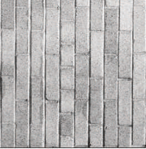
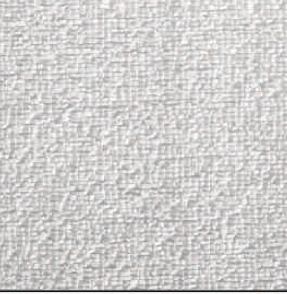
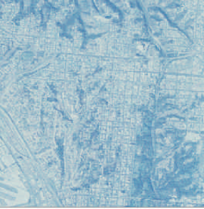
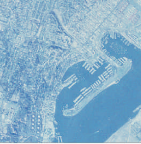
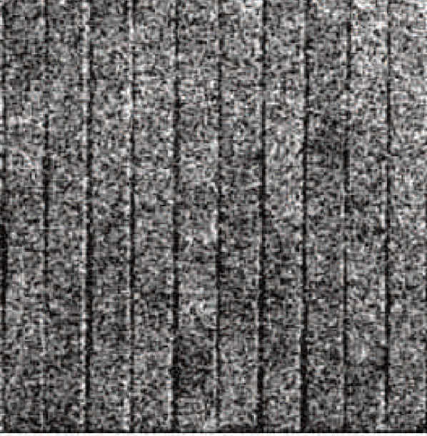
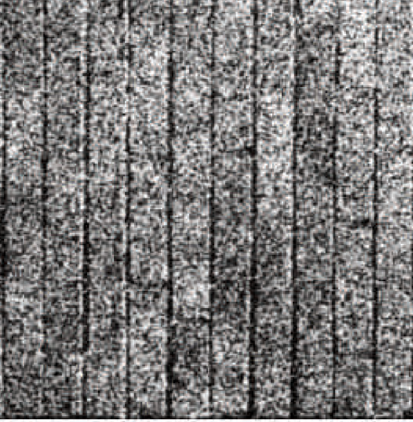
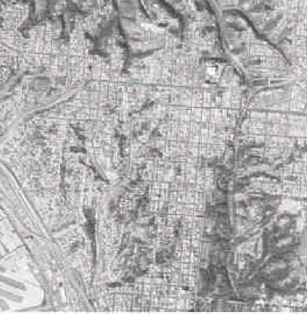
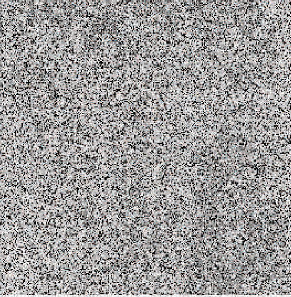
We used three sets of images, textures, aerials and miscellaneous, from the USC-SIPI Image Database¹¹1http://sipi.usc.edu/database/ as test images. Tab. 1 lists the details of the image sets, and Fig. 1 presents six sample images from the test sets.

These datasets are, in terms of contents and properties of images, very different from each other. For instance, most of the images in the texture set have highly repetitive patterns that are not present in the images in the other two sets. Most images in the aerials set have both coarse and fine structures, for example, a lake and a nearby road, at the same time in a single image. Also, the sizes of the images vary quite a lot across the test sets and across the images in each set.

Set	# of all images	# of color images	Min. Size	Max. Size
Textures	64	0	$512\times 512$	$1024\times 1024$
Aerials	38	37	$512\times 512$	$2250\times 2250$
Miscellaneous	44	16	$256\times 256$	$1024\times 1024$

Table 1: Descriptions of the test image sets.

Refer to caption — Figure 1: Sample images from the test image sets

As we are aiming to evaluate the performance of denoising a very general image, we used a large separate data set of natural image patches to train the models. We extracted a set of $100,000$ random image patches of sizes $4\times 4$ , $8\times 8$ and $16\times 16$ from CIFAR-10 dataset (Krizhevsky, 2009). From each image of $50,000$ training samples of the CIFAR-10 dataset, two patches from randomly selected locations have been collected.

We tried denoising only grayscale images. When an image was in an RGB format, we averaged the three channels to make the image grayscale.

4.2 Denoising Settings

We tried three different depth settings for both Boltzmann machines and denoising autoencoders; a single hidden layer, two hidden layers and four hidden layers. The sizes of all hidden layers were set to have the same number of hidden units, which was the constant factor multiplied by the number of pixels in an image patch²²2We used 5 as suggested by Xie et al. (2012)..

We denote Boltzmann machines with one, two and four hidden layers by GRBM, GDBM(2) and GDBM(4), respectively. Denoising autoencoders are denoted by DAE, DAE(2) and DAE(4), respectively. For each model structure, Each model was trained on image patches of sizes $4\times 4$ , $8\times 8$ and $16\times 16$ .

The GRBMs were trained using the enhanced gradient (Cho et al., 2011c) and persistent contrastive divergence (PCD) (Tieleman, 2008). The GDBMs were trained by PCD after initializing the parameters with a two-stage pretraining algorithm (Cho et al., 2012). DAEs were trained by a stochastic backpropagation algorithm, and when there were more than one hidden layers, we pretrained each layer as a single-layer DAE with sparsity target set to $0.1$ (Vincent et al., 2010; Lee et al., 2008).

The details on training procedures are described in Appendix A.

One important difference to the recent work by Xie et al. (2012) and Burger et al. (2012) is that the denoising task we consider in this paper is completely blind. No prior knowledge about target images and the type or level of noise was assumed when training the deep neural networks. In other words, no separate training was done for different types or levels of noise injected to the test images. Unlike this, Xie et al. (2012), for instance, trained a DAE specifically for each noise level by changing $\eta(\cdot)$ accordingly. Furthermore, the Boltzmann machines that we propose here for image denoising, do not require any prior knowledge about the level or type of noise.

Two types of noise have been tested; white Gaussian and salt-and-pepper. White Gaussian noise simply adds zero-mean normal random value with a predefined variance to each image pixel, while salt-and-pepper noise sets a randomly chosen subset of pixels to either black or white. Furthermore, three different noise levels (0.1, 0.2 and 0.4) were tested. In the case of white Gaussian noise, they were used as standard deviations, and in the case of salt-and-pepper noise, they were used as a noise probability.

After noise was injected, each image was preprocessed by pixel-wise adaptive Wiener filtering (see, e.g., Sonka et al., 2007), following the approach of Hyvärinen et al. (1999). The width and height of the pixel neighborhood were chosen to be small enough ( $3\times 3$ ) so that it will not remove too much detail from the input image.

Denoising performance was measured mainly with peak signal-to-noise ratio (PSNR) computed by $-10\log_{10}(\epsilon^{2}),$ where $\epsilon^{2}$ is a mean squared error between an original clean image and the denoised one.

4.3 Results and Analysis

White noise

Salt-and-pepper noise

Aerials

\psfrag{DAE}[Bl][Bl][0.7][0]{DAE}\psfrag{sDAE2}[Bl][Bl][0.7][0]{DAE(2)}\psfrag{sDAE4}[Bl][Bl][0.7][0]{DAE(4)}\psfrag{WienerFilt}[Bl][Bl][0.7][0]{Wiener Filt}\psfrag{GRBM}[Bc][Bc][0.7][0]{GRBM}\psfrag{GDBM2}[Bl][Bl][0.7][0]{GDBM(2)}\psfrag{GDBM4}[Bl][Bl][0.7][0]{GDBM(4)}\psfrag{GRBM}[Bl][Bl][0.7][0]{GRBM}\psfrag{PSNR}[Bc][Bc][0.8][0]{PSNR}\psfrag{Noise Level}[Tc][Tc][0.8][0]{Noise Level}\psfrag{0.1}[Tc][Tc][0.8][0]{$0.1$}\psfrag{0.2}[Tc][Tc][0.8][0]{$0.2$}\psfrag{0.3}[Tc][Tc][0.8][0]{$0.3$}\includegraphics[width=433.62pt]{psnr_white_aerials.eps}

Textures

Misc.

Figure 2: PSNR of grayscale images corrupted by different types and levels of noise. The median PSNRs over the images in each set together.

In Fig. 2, the performances of all the tested models trained on $8\times 8$ image patches are presented³³3Those trained on patches of different sizes showed similar trend, and they are omitted in this paper. .

The most obvious observation is that the deep neural networks, including both DAEs and BMs, did not show improvement over their shallow counterparts in the low-noise regime (0.1). However, the deeper models significantly outperformed their corresponding shallow models as the level of injected noise grew. In other words, the power of the deep models became more evident as the injected level of noise grew.

This is supported further by Tab. 2 which shows the performance of the models in the high noise regime (0.4). In all cases, the deeper models, such as DAE(4), GDBM(2) and GDBM(4), were the best performing models.

Another notable phenomenon is that the GDBMs tend to lag behind the DAEs, and even the GRBM, in the low noise regime, except for the textures set. A possible explanation for this rather poor performance of the GDBMs in the low noise regime is that the approximate inference of the posterior distribution, used in this experiment, might not have been good enough. For instance, more mean-field iterations might have improved the overall performance while dramatically increasing the computational time, which would not allow GDBMs to be of any practical value. The GDBMs, however, outperformed, or performed comparably to, the other models when the level of injected noise was higher.

It should be noticed that the performance depended on the type of the test images. For instance, although the images in the aerials set corrupted with salt-and-pepper noise were best denoised by the DAE with four hidden layers, the GDBMs outperformed the DAE(4) in the case of the textures set. We emphasize here that the deeper neural networks showed less performance variance depending on the type of test images, which suggests better generalization capability of the deeper neural networks.

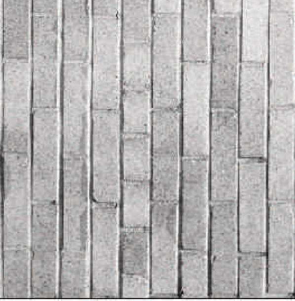
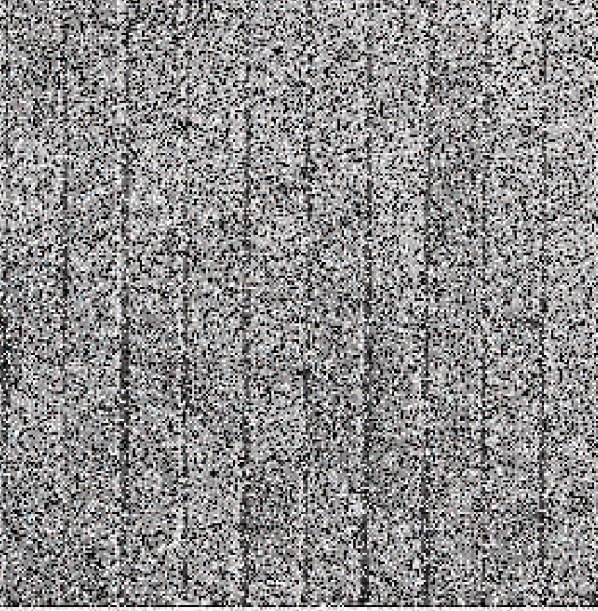
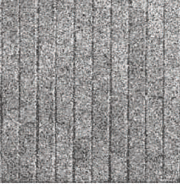
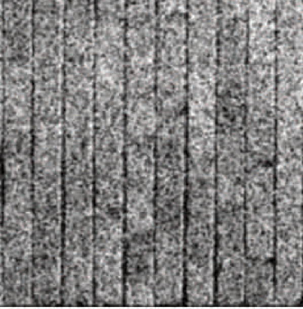
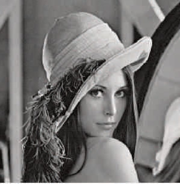
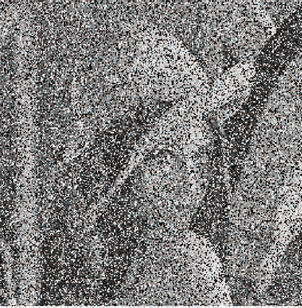
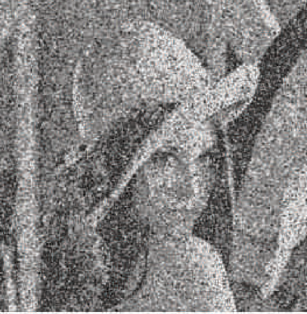
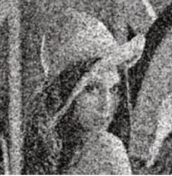
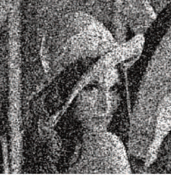
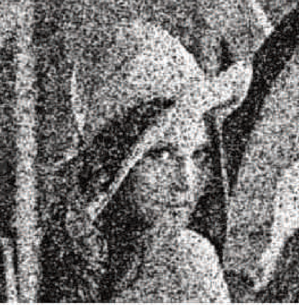
Visual inspection of the denoised images provides some more intuition on the performances of the deep neural networks. In Fig. 3, the denoised images of a sample image from each test image set are displayed. It shows that BMs tend to emphasize the detailed structure of the image, while DAEs, especially ones with more hidden layers, tend to capture the global structure.

Additionally, we tried the same set of experiments using the models trained on a set of $50,000$ random image patches extracted from the Berkeley Segmentation Dataset Martin et al. (2001). In this case, $100$ patches from randomly chosen locations from each of $500$ images were collected to form the training set. We obtained the results similar to those presented in this paper. The results are presented in Appendix B.

Method	Aerials	Textures	Misc.
Wiener	15.7 (0.1)	15.5 (0.6)	15.9 (0.6)
DAE	16.4 (0.2)	16.2 (0.9)	16.6 (0.8)
DAE(2)	17.6 (0.2)	17.1 (1.2)	17.7 (1.1)
DAE(4)	20.8 (0.7)	18.7 (2.8)	20.2 (2.0)
GRBM	19.2 (0.4)	18.0 (1.7)	18.9 (1.5)
GDBM(2)	22.3 (1.4)	18.7 (3.2)	20.1 (2.4)
GDBM(4)	22.1 (1.1)	18.7 (3.0)	20.2 (2.2)

Aerials	Textures	Misc.
16.3 (0.5)	14.9 (1.3)	15.3 (1.5)
17.1 (0.6)	15.7 (1.4)	16.3 (1.7)
18.1 (0.7)	16.4 (1.7)	17.3 (2.0)
20.1 (1.1)	17.2 (2.8)	19.0 (2.7)
18.9 (0.9)	16.6 (2.1)	17.6 (2.2)
20.3 (1.4)	16.5 (3.0)	17.5 (2.6)
20.3 (1.3)	16.6 (2.9)	17.6 (2.5)

(a) White Gaussian Noise

(b) Salt-and-Pepper Noise

Table 2: Performance of the models trained on

4\times 4

image patches when the level of injected noise was 0.4. Standard deviations are shown inside the parentheses, and the best performing models are marked bold.

5 Conclusion

In this paper, we proposed that, in addition to DAEs, Boltzmann machines, GRBMs and GDBMS, can also be used for denoising images. Furthermore, we tried to find empirical evidence supporting the use of deep neural networks in image denoising tasks.

Our experiments suggest the following conclusions for the questions raised earlier:

Does a model with more hidden layers perform better?

In the case of DAEs, the experiments clearly show that more hidden layers do improve performance, especially when the level of noise is high. This does not always apply to BMs, where we found that the GRBMs outperformed, or performed as well as, the GDBMs in few cases. Regardlessly, in the high noise regime, it was always beneficial to have more hidden layers.

How well does a deep model generalize?

The deep neural networks were trained on a completely separate dataset and were applied to three test sets with very different image properties. It turned out that the performance depended on each test set, however, with only small differences. Also, the trend of deeper models performing better could be observed in almost all cases, again especially with high level of noise. This suggests that a well-trained deep neural network can perform blind image denoising, where no prior information about target, noisy images is available, well.

Which family of deep neural networks is more suitable, BMs or DAEs?

The DAE with four hidden layers turned out to be the best performer, in general, beating GDBMs with the same number of hidden layers. However, when the level of noise was high, the Boltzmann machines such as GRBM and GDBM(2) were able to outperform the DAEs, which suggests that Boltzmann machines are more robust to noise.

One noticeable observation was that the GRBM outperformed, in many cases, the DAE with two hidden layers which had twice as many parameter. This potentially suggests that a better inference of approximate posterior distribution over the hidden units might make GDBMs outperform, or comparable to, DAEs with the same number of hidden layers and units. More work will be required in the future to make a definite answer to this question.

Although it is difficult to make any general conclusion from the experiments, it was evident that deep models, regardless of whether they are DAEs or BMs, performed better and were more robust to the level of noise than their more shallow counterparts. In the future, it might be appealing to investigate the possibility of combining multiple deep neural networks with various depths to achieve better denoising performance.

References

Ackley et al. [1985] David H. Ackley, Geoffrey E. Hinton, and Terrence J. Sejnowski. A learning algorithm for Boltzmann machines. Cognitive Science, 9:147–169, 1985.
Burger et al. [2012] H.C. Burger, C.J. Schuler, and S. Harmeling. Image denoising: Can plain neural networks compete with bm3d? In Computer Vision and Pattern Recognition (CVPR), 2012 IEEE Conference on, pages 2392 –2399, june 2012.
Cho et al. [2013] K. Cho, T. Raiko, and A. Ilin. Enhanced gradient for training restricted Boltzmann machines. Neural Computation, 2013.
Cho et al. [2011a] KyungHyun Cho, Alexander Ilin, and Tapani Raiko. Improved learning of Gaussian-Bernoulli restricted Boltzmann machines. In Proc. of the 20th Int. Conf. on Artificial Neural Networks (ICANN 2010), 2011a.
Cho et al. [2011b] KyungHyun Cho, Tapani Raiko, and Alexander Ilin. Gaussian-Bernoulli deep Boltzmann machine. In NIPS 2011 Workshop on Deep Learning and Unsupervised Feature Learning, Sierra Nevada, Spain, December 2011b.
Cho et al. [2011c] KyungHyun Cho, Tapani Raiko, and Alexander Ilin. Enhanced gradient and adaptive learning rate for training restricted Boltzmann machines. In Proc. of the 28th Int. Conf. on Machine Learning (ICML 2011), pages 105–112, New York, NY, USA, June 2011c. ACM.
Cho et al. [2012] KyungHyun Cho, Tapani Raiko, Alexander Ilin, and Juha Karhunen. A Two-Stage Pretraining Algorithm for Deep Boltzmann Machines. In NIPS 2012 Workshop on Deep Learning and Unsupervised Feature Learning, Lake Tahoe, December 2012.
Dabov et al. [2007] Kostadin Dabov, Alessandro Foi, Vladimir Katkovnik, and Karen Egiazarian. Image denoising by sparse 3-D Transform-Domain collaborative filtering. Image Processing, IEEE Transactions on, 16(8):2080–2095, August 2007.
Desjardins et al. [2012] Guillaume Desjardins, Aaron C. Courville, and Yoshua Bengio. On training deep Boltzmann machines. CoRR (Cornell Univ. Computing Research Repository), abs/1203.4416, 2012.
Elad and Aharon [2006] M. Elad and M. Aharon. Image denoising via sparse and redundant representations over learned dictionaries. Image Processing, IEEE Transactions on, 15(12):3736–3745, December 2006.
Hinton and Salakhutdinov [2006] G. Hinton and R. Salakhutdinov. Reducing the dimensionality of data with neural networks. Science, 313(5786):504–507, July 2006.
Hinton [2002] Geoffrey Hinton. Training products of experts by minimizing contrastive divergence. Neural Computation, 14:1771–1800, August 2002.
Hyvärinen et al. [1999] Aapo Hyvärinen, Patrik Hoyer, and Erkki Oja. Image denoising by sparse code shrinkage. In Intelligent Signal Processing. IEEE Press, 1999.
Krizhevsky [2009] A. Krizhevsky. Learning multiple layers of features from tiny images. Technical report, Computer Science Department, University of Toronto, 2009.
Lee et al. [2008] Honglak Lee, Chaitanya Ekanadham, and Andrew Ng. Sparse deep belief net model for visual area V2. pages 873–880, 2008.
Lu et al. [2011] Xiaoqiang Lu, Haoliang Yuan, Pingkun Yan, Luoqing Li, and Xuelong Li. Image denoising via improved sparse coding. In Proceedings of the British Machine Vision Conference, pages 74.1–74.0. BMVA Press, 2011.
Martin et al. [2001] D. Martin, C. Fowlkes, D. Tal, and J. Malik. A database of human segmented natural images and its application to evaluating segmentation algorithms and measuring ecological statistics. In Proc. 8th Int’l Conf. Computer Vision, volume 2, pages 416–423, July 2001.
Neal and Hinton [1999] Radford M. Neal and Geoffrey E. Hinton. Learning in graphical models. chapter A view of the EM algorithm that justifies incremental, sparse, and other variants, pages 355–368. MIT Press, Cambridge, MA, USA, 1999.
Portilla et al. [2003] J. Portilla, V. Strela, M.J. Wainwright, and E.P. Simoncelli. Image denoising using scale mixtures of gaussians in the wavelet domain. Image Processing, IEEE Transactions on, 12(11):1338 – 1351, nov. 2003.
Salakhutdinov [2010] Ruslan Salakhutdinov. Learning deep Boltzmann machines using adaptive MCMC. In Johannes Fürnkranz and Thorsten Joachims, editors, Proc. of the 27th Int. Conf. on Machine Learning (ICML 2010), pages 943–950, Haifa, Israel, June 2010. Omnipress.
Salakhutdinov and Hinton [2009] Ruslan Salakhutdinov and Geoffrey E. Hinton. Deep Boltzmann machines. In Proc. of the Int. Conf. on Artificial Intelligence and Statistics (AISTATS 2009), pages 448–455, 2009.
Shang and Huang [2005] Li Shang and Deshuang Huang. Image denoising using non-negative sparse coding shrinkage algorithm. In Computer Vision and Pattern Recognition, 2005. CVPR 2005. IEEE Computer Society Conference on, volume 1, pages 1017 – 1022 vol. 1, june 2005.
Smolensky [1986] P. Smolensky. Information processing in dynamical systems: foundations of harmony theory. In Parallel distributed processing: explorations in the microstructure of cognition, vol. 1: foundations, pages 194–281. MIT Press, Cambridge, MA, USA, 1986.
Sonka et al. [2007] Milan Sonka, Vaclav Hlavac, and Roger Boyle. Image Processing, Analysis, and Machine Vision. Thomson-Engineering, 2007. ISBN 049508252X.
Tieleman [2008] Tijmen Tieleman. Training restricted Boltzmann machines using approximations to the likelihood gradient. ICML ’08. ACM, New York, NY, USA, 2008.
Vincent et al. [2010] Pascal Vincent, Hugo Larochelle, Isabelle Lajoie, Yoshua Bengio, and Pierre-Antoine Manzagol. Stacked denoising autoencoders: Learning useful representations in a deep network with a local denoising criterion. Journal of Machine Learning Research, 11:3371–3408, December 2010.
Xie et al. [2012] Junyuan Xie, Linli Xu, and Enhong Chen. Image denoising and inpainting with deep neural networks. In P. Bartlett, F.C.N. Pereira, C.J.C. Burges, L. Bottou, and K.Q. Weinberger, editors, Advances in Neural Information Processing Systems 25, pages 350–358. 2012.

Appendix A Training Procedures: Details

Here, we describe the procedures used for training the deep neural networks in the experiments.

A.1 Data Preprocessing

Prior to training a model, we normalized each pixel of the training set such that, across all the training samples, the mean and variance of each pixel are $0$ and $1$ .

The original mean and variance were discarded after training. During test, we computed the mean and variance of all image patches from each test image and used them instead.

A.2 Denoising Autoencoders

A single-layer DAE was trained by the stochastic gradient descent for 200 epochs. A minibatch of size 128 was used at each update, and a single epoch was equivalent to one cycle over all training samples.

The initial learning rate was set to $\eta_{0}=0.05$ and was decreased over training according to the following schedule:

\displaystyle\eta_{t}=\frac{\eta_{0}}{1+\frac{t}{5000}}.

In order to encourage the sparsity of the hidden units, we used the following regularization term

\displaystyle-\lambda\sum_{n=1}^{N}\sum_{j=1}^{q}\left(\rho-\phi\left(\sum_{i=1}^{p}v_{i}^{(n)}w_{ij}+c_{j}\right)\right)^{2},

where $\lambda=0.1$ , $\rho=0.1$ and $p$ and $q$ are respectively the numbers of visible and hidden units. $\phi$ is a sigmoid function.

Before computing the gradient at each update, we added a white Gaussian noise of standard deviation $0.1$ to all components of an input sample and forced randomly chosen 20% of input units to zeros.

The weights of a deep DAE was first initialized by layer-wise pretraining. During the pretraining, each layer was trained as if it were a single-layer DAE, following the same procedure described above, except that no white Gaussian noise was added for the layers other than the first one.

After pretraining, we trained the deep DAE with the stochastic backpropagation algorithm for 200 epochs using minibatches of size 128. The initial learning rate was chosen to be $\eta_{0}=0.01$ and the learning rate was annealed according to

\displaystyle\eta_{t}=\frac{\eta_{0}}{1+\frac{t}{5000}}.

For each denoising autoencoder regardless of its depth, we used a tied set of weights for the encoder and decoder.

A.3 Restricted Boltzmann Machines

We used the modified energy function of a Gaussian-Bernoulli RBM (GRBM) proposed by Cho et al. [2011a], however, with a single $\sigma^{2}$ shared across all the visible units. Each GRBM was trained for 200 epochs, and each update was performed using a minibatch of size 128.

A learning rate was automatically selected by the adaptive learning rate [Cho et al., 2011a] with the initial learning rate and the upper-bound fixed to $0.001$ and $0.001$ , respectively. After 180 epochs, we decreased the learning rate according to

\eta\leftarrow\frac{\eta}{t},

where $t$ denotes the number of updates counted after 180 epochs of training.

A persistent contrastive divergence (PCD) [Tieleman, 2008] was used, and at each update, a single Gibbs step was taken for the model samples. Together with PCD, we used the enhanced gradient [Cho et al., 2013], instead of the standard gradient, at each update.

A.4 Deep Boltzmann Machines

We used the two-stage pretraining algorithm [Cho et al., 2012] to initialize the parameters of each DBM. The pretraining algorithm consists of two separate stages.

We utilized the already trained single-layer and two-layer DAEs to compute the activations of the hidden units in the even-numbered hidden layers of GDBMs. No separate, further training was done for those DAEs in the first stage.

In the second stage, the model was trained as an RBM using the coupled adaptive simulated tempering [CAST, Salakhutdinov, 2010] with the base inverse temperature set of $0.9$ and $50$ intermediate chains between the base and model distributions. At least 50 updates were required to make a swap between the slow and fast samples.

The initial learning rate was set to $\eta_{0}=0.01$ and the learning rate was annealed according to

\eta_{t}=\frac{\eta_{0}}{1+\frac{t}{5000}}.

Again, the modified form of an energy function [Cho et al., 2011b] was used with a shared variance $\sigma^{2}$ for all the visible units. However, in this case, we did not use the enhanced gradient.

After pretraining, the GDBMs were further finetuned using the stochastic gradient method together with the variational approximation [Salakhutdinov and Hinton, 2009]. The CAST was again used with the same hyperparameters. The initial learning rate was set to $0.0005$ and the learning rate was decreased according to the same schedule used during the second stage.

Appendix B Result Using a Training Set From Berkeley Segmentation Dataset

Fig. 4 shows the result obtained by the models trained on the training set constructed from the Berkeley Segmentation Dataset. Although we see some minor differences, the overall trend is observed to be similar to that from the experiment in the main text (see Fig. 2).

Especially in the high-noise regime, the models with more hidden layers tend to outperform those with only one or two hidden layers. This agrees well with what we have observed with the models trained on the training set constructed from the CIFAR-10 dataset.