Fitting Methods for Baryon Acoustic Oscillations in the Lyman- Forest Fluctuations in BOSS Data Release 9
Abstract
We describe fitting methods developed to analyze fluctuations in the Lyman- forest and measure the parameters of baryon acoustic oscillations (BAO). We apply our methods to BOSS Data Release 9. Our method is based on models of the three-dimensional correlation function in physical coordinate space, and includes the effects of redshift-space distortions, anisotropic non-linear broadening, and broadband distortions. We allow for independent scale factors along and perpendicular to the line of sight to minimize the dependence on our assumed fiducial cosmology and to obtain separate measurements of the BAO angular and relative velocity scales. Our fitting software and the input files needed to reproduce our main BOSS Data Release 9 results are publicly available.
1 Introduction
The surprising discovery [1, 2] of accelerating expansion in the current universe reveals that either some form of dark energy is driving the expansion or else that our theory of gravity is incomplete on the largest scales (see reference [3] for a recent review). The length scale of baryon acoustic oscillations (BAO) imprinted at the moment of baryon-photon decoupling provides a standard ruler that has been well measured in the temperature anisotropies of the cosmic microwave background [4, 5] (CMB) and in the number-density fluctuations of galaxies at [6, 7, 8, 9, 10, 11, 12, 13, 14, 15, 16, 17, 18, 19, 20, 21, 22, 23, 24]. The Baryon Oscillation Spectroscopic Survey [25] (BOSS) of the third generation of the Sloan Digital Sky Survey [26] (SDSS-III) recently announced its ninth data release [27] (DR9), including an unprecedented number of high-redshift quasar spectra. The BAO feature is imprinted in the correlated fluctuations of intergalactic Lyman- absorption of the light from these quasars, enabling us to measure the BAO standard ruler at redshifts , during the predicted era of matter-dominated deceleration.
An optimal extraction of the BAO signal from a large sample of Lyman- forest pixels requires new fitting techniques beyond those previously developed to fit the large-scale clustering of galaxies [28]. For example, the non-uniform sampling of the absorption field, large expected redshift-space distortions, and relatively large depth suggest that estimates of the correlation function or power spectrum should be fit to three-dimensional models (rather than low-order multipoles at fixed redshift) expressed directly in terms of the physical absorption wavelengths and angular separations between lines of sight. We describe here new fitting techniques developed specifically for a near-optimal analysis of the DR9 correlation-function estimates described in a companion paper [29], and highlight the challenges and lessons learned. We are also making our fit input files and fitting code publicly available as a companion to this paper, so that readers may reproduce the main results presented here and in ref. [29].
The outline of our paper is as follows. In Section 2 we define our constituent models for linear theory with redshift-space distortions, non-linear effects, and redshift evolution. We also describe our parametrizations of possible deviations between our assumed fiducial cosmology111We assume a flat CDM universe with , , , and throughout. and the cosmology preferred by our data, and of broadband distortion of our correlation-function estimate introduced by analysis systematics. Finally, we introduce two data-reduction techniques using interpolated models. In Section 3, we describe the DR9 fitting inputs which consist of correlation-function estimates on a three-dimensional physical coordinate grid, accompanied by an initial estimate of their covariance in a block diagonal form that reduces the number of non-zero elements from K to K. Next, we describe a novel method for internally validating and refining our initial covariance estimate, necessitated by a lack of available simulated mock statistics. In Section 4, we present our results on the fitting method and what it teaches us about the BOSS DR9 Lyman- forest dataset. We discuss the expected parameter sensitivities and relative contributions from different regions of the three-dimensional separation space, and present model-independent data reduction results. Cosmological fitting results for DR9 are presented in the companion paper ref. [29]. We conclude in Section 5 with a discussion of the main lessons learned and our plans for future development. Appendix A provides details on public access to our fit inputs and fitting code.
2 Models and Parameters
We model a measurement of the correlation function
| (2.1) |
where the ensemble averages are taken over realizations of a (possibly biased) tracer of the large-scale distribution of matter in redshift space , with defined via222We use the notation and .
| (2.2) |
for some fiducial cosmology with Hubble function . The model combines a cosmological prediction with a parametrization of possible multiplicative and additive broadband distortions introduced by the analysis method.
2.1 Physical Coordinates
The physical coordinates for a pair of pixels measured in the absorption spectra of two quasars are the separation angle between the quasar lines of sight ( if the pixels are taken from the same quasar’s spectrum) and the observed absorption wavelengths and . We convert the observed wavelengths to a relative velocity for the absorption systems333This definition is not identical to the Doppler velocity that an observer at one absorber would measure for the other absorber, but does agree to second order in the wavelength ratio. [30]
| (2.3) |
and an average absorption redshift
| (2.4) |
where Å is the rest wavelength of the Lyman- transition which determines pixel redshifts . We calculate the corresponding co-moving separations along () and perpendicular to () the line of sight as
| (2.5) | ||||
| (2.6) |
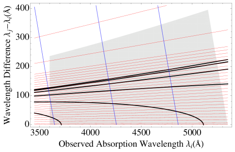
where and are the co-moving line of sight and angular distance functions, respectively, for the assumed fidicual cosmology . We introduce separate scale factors and in Section 2.2.4 to allow for small discrepancies between the true cosmology and our assumed fiducial model. Fig 1 shows that the BOSS blue camera wavelength limit of Å limits pixel pairs contributing to a BAO peak feature near 110 Mpc/h to arcmin. Similarly, the BOSS redshift coverage limits the BAO peak to and observed wavelength differences Å.
2.2 Cosmological Models
We build the cosmological model starting from an isotropic linear power spectrum prediction at some reference redshift , then embed this prediction in redshift space (we use tildes to denote linear-theory predictions without any redshift space distortions). In the general case of a plane-parallel redshift-space distortion we have [31]:
| (2.7) |
with
| (2.8) |
where is the Legendre polynomial, is the spherical Bessel function, and are the multipoles of the redshift-distorted power spectrum with :
| (2.9) |
Specializing to linear theory and the distant observer approximation [32], the infinite series of eqn. (2.7) is truncated at , with
| (2.10) |
and
| (2.11) |
where and are the tracer bias and redshift-space distortion parameter at redshift , respectively. We can therefore write
| (2.12) |
in terms of the undistorted linear-theory multipoles
| (2.13) |
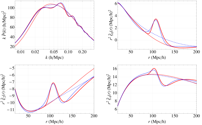
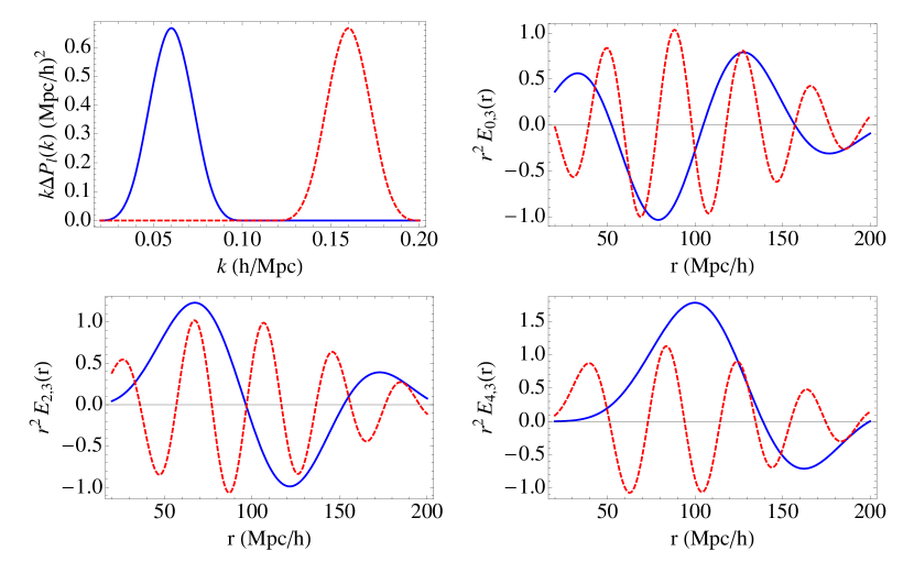
Figure 2 shows examples of the linear models we use for Lyman- fitting in this paper, calculated with . Note that the undistorted multipoles are not independent since they derive from the same underlying power spectrum via eqn. (2.13). Explicitly, we find that and can be calculated directly from specified on an interval via (we have dropped here for clarity):
| (2.14) | ||||
where is an arbitrarily chosen scale and the influence of scales beyond is fully specified by the constants of integration .
2.2.1 Peak Decomposition
We expect a Lyman- analysis to distort the measured broadband shape of the correlation function, so our goal is to only use information from the localized peak near Mpc/h to measure BAO parameters. To achieve this goal, it is useful to decompose into separate “peak” and “smooth” (or “no-wiggles”) components. Following ref. [34], we can isolate the oscillations in a multiplicative term of the effective baryon transfer function (see equation (16) in ref. [34]), which leads to a rather complicated decomposition for the correlation function. Instead, we adopt the unphysical but more tractable decomposition
| (2.15) |
with the understanding that this model is only valid when using parameter values that are sufficiently close to their nominal values to recover a physically plausible .
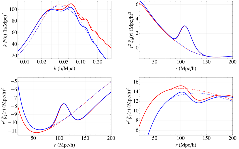
Figure 2 shows the smooth and corresponding correlation multipoles suggested in ref. [34]: the oscillations are effectively removed, but the corresponding “peak” feature, defined as the difference between the full and “no-wiggles” models, is not well localized in any of the multipoles, with deviations from the dashed curves extending far from the peak. To remedy this problem, we construct an alternate peak model that is explicitly localized, but only for a single linear combination of multipoles (or, equivalently, a single value of ) because the integrals in eqn. (2.14) effectively spread the peak to all scales above and/or below (depending on the choice of ) for other linear combinations. Our CAMB “sideband” smooth model is constructed as follows: we first isolate a localized peak in the CAMB prediction [33] of Figure 2 by simultaneously fitting the regions 50–86 and 150–190 Mpc/h of the monopole to the form
| (2.16) |
Next, we replace with in the region 86–150 Mpc/h to obtain . We then calculate and using eqn. (2.14) with at . Finally, we calculate
| (2.17) |
The resulting CAMB “sideband” smooth model is shown in Figure 2.
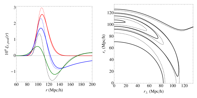
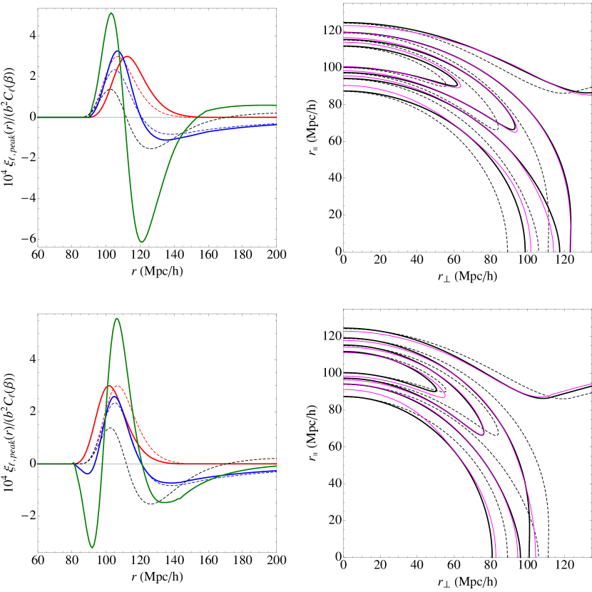
By construction, our CAMB peak multipoles are exactly zero below 86 Mpc/h, but the peak spreads to large scales for , as required by eqn. (2.14). Note that although it would be possible to specify independent localized peaks for each multipole, this is unphysical (within the framework of ref. [32]) and does not, in general, reproduce the evolution of the peak shape in with implied by the constraint of a single underlying , as illustrated in Figure 3. For example, the constrained evolution leads to a percent-level shift in the peak position as a function of shown in Figure 4 for the two models used here. Note that this shift is essentially the same for both models, despite the rather different peak shapes shown in Figure 3.


2.2.2 Nonlinear Effects
The expected effects of non-linear structure growth on the BAO feature can be modeled with an anisotropic Gaussian roll-off of the linear power spectrum [35]:
| (2.18) |
where
| (2.19) |
In general, this approach breaks the decomposition, eqn. (2.10), of into separate - and -dependent factors and requires that the integrals of eqns. (2.8)–(2.9) be re-evaluated for each value of . However, since we expect Mpc/h, compared with an expected peak full-width half-maximum of Mpc/h, we can approximate for :
| (2.20) |
with
| (2.21) |
and
| (2.22) |
This approximation effectively models anisotropic broadening using different amounts of isotropic broadening for each multipole. The resulting correlation function multipoles , calculated with eqn. (2.8), can then be substituted in eqn. (2.12).
Taking a fiducial value of , we calculate , , and . At a redshift , we expect Mpc/h and Mpc/h, so that Mpc/h, Mpc/h, and Mpc/h. Figure 5 compares the resulting approximate models with exact calculations for a range of values. Note that we are neglecting the non-zero even multipoles that are introduced by anisotropic non-linear broadening with this approximation, but Fig 5 shows that most of the BAO peak feature has already been smoothed out by . We also neglect any redshift evolution of the non-linear broadening parameters, since this evolution would be a second order effect on what is already a small correction to the linear theory for the purposes of measuring the BAO feature.
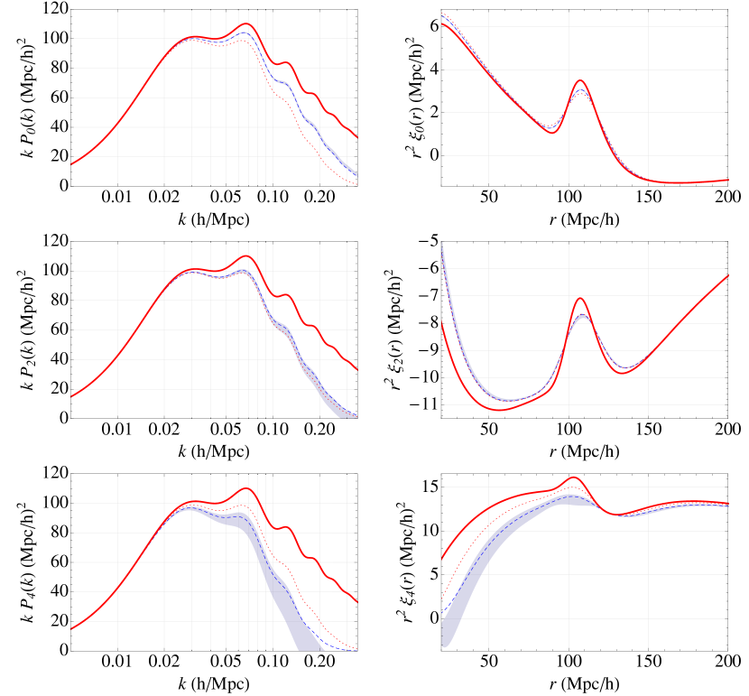
In order to achieve a self-consistent decomposition of each correlation-function multipole into peak + smooth components with non-linear broadening effects included, we first broaden each by to obtain . Broadening by in this context implies
| (2.23) |
which transforms to
| (2.24) |
where is the normalized one-dimensional Gaussian
| (2.25) |
Note that when , we recover the expected convolution
| (2.26) |
to a good approximation. Figure 6 shows the broadened multipole peaks based on our linear CAMB templates. To derive the corresponding smooth templates, we either use the linear smooth templates, or else we calculate non-linear smooth templates by subtracting the broadened peak templates from the broadened multipoles:
| (2.27) |
In the first case, we are only applying non-linear broadening to the peak feature, which introduces an unphysical distinction between peak and smooth components. In the second case we are broadening the full correlation function, which removes the distinction but applies unphysical filtering of small scale structure. A better model is probably somewhere in between so we consider both alternatives, and expect that any extracted peak parameters will not depend on this choice. Figure 7 compares both approaches.
2.2.3 Redshift Evolution
In general, we model the redshift evolution of a parameter for near in terms of two parameters and via
| (2.28) |
We apply this evolution to the parameters and , introduced above, and to the BAO scale parameters , and introduced below. Given a covariance matrix for the parameters and ,
| (2.29) |
the variance of with is given by
| (2.30) |
where
| (2.31) |
is the Jacobian. The error on is smallest at
| (2.32) |
with
| (2.33) |
2.2.4 Scale Factors
When fitting our model to data, we allow for an overall relative normalization factor as well as a general coordinate transform, and , that allows for possible small differences444In case there is evidence for large differences, the analysis should be repeated with a fidicual cosmology that better matches the data. between the fiducial and actual cosmologies:
| (2.34) |
We consider two options for the cosmological broadband : we either apply the same transform as for the peak (), or else we keep it fixed () so that only the peak is transformed. Neither approach is exact when considering variations of the cosmological parameters around our fidicual model, but we find that decoupling the peak from the cosmological broadband () better localizes the separations contributing to a BAO measurement to the peak region (compare Figs. 16 and 19), so is preferred when broadband distortion is not fully under control. The corresponding -space transforms are defined by
| (2.35) |
Including a -dependence in the coordinate transform also enables us to study the constraining power of our data separately along and transverse to the line of sight. Similarly, a -dependence allows us to determine the redshift at which our results are best measured using eqn. (2.32).
For our baseline isotropic model, we use
| (2.36) | ||||
For our baseline anisotropic model, we decouple the line-of-sight () and transverse () scales using
| (2.37) | ||||
with
| (2.38) |
When the parameters of this anisotropic model are determined by measuring the physical coordinate separation scales and corresponding to the comoving BAO scale at some redshift , related by
| (2.39) | ||||
| (2.40) |
then the expected best fit values of and satisfy
| (2.41) | ||||
| (2.42) |
where is the comoving BAO scale predicted by the assumed fiducial cosmology. Combining these results, the best-fit anisotropic scale factors measure
| (2.43) |
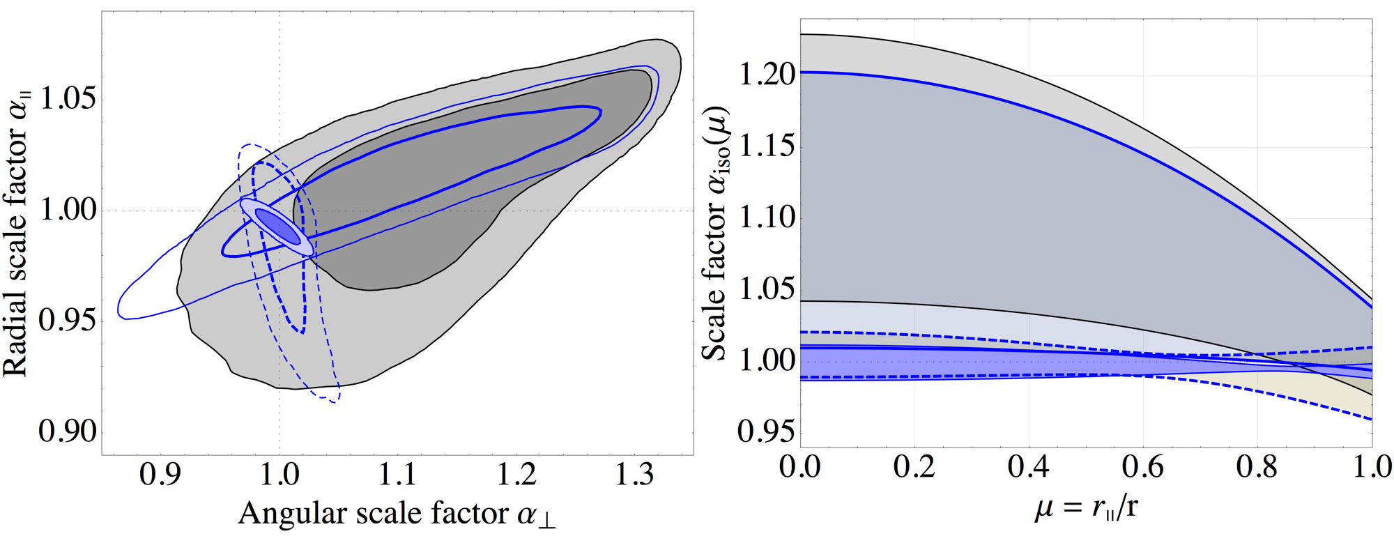
The distributions of these ratios predicted at by WMAP9 [4] observations of the CMB are shown in Figure 8.
We can evaluate a transformed correlation function in the original coordinates using eqn. (2.12) (with -dependencies omitted for clarity)
| (2.44) | ||||
The corresponding multipoles in the original coordinates are then given by
| (2.45) | ||||
| (2.46) |
In the case of isotropic distortion, we can simply replace with in the multipoles obtained with eqn. (2.13). However, anisotropic distortions mix multipoles and lead to more complicated expressions. For small and arbitrary , we have
| (2.47) |
and corresponding transforms
| (2.48) | |||||
Using these approximations, and
| (2.49) |
we obtain distorted multipoles:
| (2.50) |
where
| (2.51) | ||||
| (2.52) |
We find the following non-zero coefficients, to first order in :
| (2.53) | |||
| (2.54) | |||
| (2.55) | |||
| (2.56) |
Note that an term must be included in order to match eqn. (2.46) to first order in , but is numerically negligible. On the other hand, second-derivative terms in the Taylor expansion 2.49 are formally but are numerically significant when
| (2.57) |
which is guaranteed to occur at the peak of the BAO feature and at the transition to a rising smooth broadband below the peak. Figure 9 shows examples of anisotropic coordinate transforms based on eqns. (2.44) and (2.50). Note that eqn. (2.50) is only exact when () and grows less accurate when moving away from the diagonal, while eqn. (2.44) is exact and therefore preferred when fitting for the anisotropic scale parameters.
2.3 Broadband Distortion Models
A Lyman- analysis measures the correlation function
| (2.58) |
for the overdensity proxy
| (2.59) |
in pixels measured at rest absorption wavelengths , where
| (2.60) |
is the transmitted flux fraction, relative to the sky flux level and normalized to an assumed quasar continuum flux level , and is an assumed mean transmission fraction at .
To investigate possible sources of broadband distortion, write
| (2.61) | ||||
where tilde quantities are true values, and are (zero-mean) noise sources, accounts for any wavelength-dependent residual sky-subtraction bias (as observed in DR9), and describes the continuum modeling error that, in general, depends on the full vector of pixel measurements
| (2.62) |
Combining eqns. (2.60) and (2.61), we find:
| (2.63) | ||||
with
| (2.64) |
where we have assumed that . Averaging over noise and cosmic realizations, we find:
| (2.65) |
where
| (2.66) |
is the undistorted cosmological correlation function we seek to measure, describes the effects of any discrepancy between the assumed and true mean transmitted flux fraction via
| (2.67) |
is a multiplicative distortion of the true correlation function
| (2.68) |
and is an additive distortion
| (2.69) |
where we have used and assumed that , , and are mutually uncorrelated.
Equation (2.65) demonstrates that, in general, the measured correlation function can be systematically distorted by multiplicative and additive effects. The actual correlation function used for fitting is a weighted sum of pixels in bins of . Any multiplicative distortion is due to a mismatch between the assumed and the true mean transmitted flux for pixels at the same wavelength , whereas additive distortion is due to correlated continuum fit errors.
We model broadband distortion using the following parametrization that combines the multiplicative () and additive () effects described above:
| (2.70) |
with ( represents either or )
| (2.71) |
where, nominally, Mpc/h and , and
| (2.72) |
The integers , , and determine the number of free parameters, and we normally restrict to even values. The multipoles of the distorted correlation function are given by (arguments of are suppressed for clarity):
| (2.73) | ||||
| (2.74) | ||||
| (2.75) |
with distortion multipoles given by
| (2.76) |
For the purposes of fitting DR9, we chose six different parameter configurations for broadband distortion, as summarized in Table 1 and plotted in Figure 10.
| Name | ||||||
|---|---|---|---|---|---|---|
| BB1 | - | - | - | 0,1,2 | 0,2,4 | 0 |
| BB2 | - | - | - | -2,-1,0 | 0,2,4 | 0 |
| BB3 | - | - | - | 0,1,2 | 0,2 | 0,1 |
| BB4 | 0,1,2 | 0,2,4 | 0 | - | - | - |
| BB5 | 0,1,2 | 0,2 | 0,1 | - | - | - |
| BB6 | 0,1 | 0,2,4 | 0 | 0,1 | 0,2,4 | 0 |
2.4 Interpolated Models
For the purposes of visualization and studying non-cosmological signatures in data, it is useful to fit using simple interpolated models with minimal assumptions. We describe here two such models: the first treats the correlation multipoles as (possibly independent) arbitrary interpolations through fixed arbitrary values of the separation, and the second treats corrections to a smoothed power spectrum as (possibly independent) arbitrary interpolations through equally spaced wave numbers covering a limited band.
For our first model, we pick fixed values of the separation and model the -weighted correlation multipoles as:
| (2.77) |
where is an -th order interpolation through the points evaluated at separation and referenced to the redshift . Comparing with eqn. (2.10), we write
| (2.78) |
so that
| (2.79) |
when is purely cosmological.
For our second model, we interpolate over a fixed band of -space and therefore require some assumption about the power outside this band in order to predict -space correlations. We adopt the following form for the multipoles of the power spectrum:
| (2.80) |
where is a smoothed fiducial power spectrum, without any BAO features, modulated by functions that are zero outside some interval , both referenced to . The correlation multipoles corresponding to eqn. (2.80) are obtained via eqn. (2.8):
| (2.81) |
with
| (2.82) |
We parameterize the -weighted modulation as a linear combination of -th order B-spline functions :
| (2.83) |
with uniformly spaced knots at:
| (2.84) |
Using the property that is only non-zero for , we can write
| (2.85) |
where
| (2.86) |
with
| (2.87) |
can be solved analytically in terms of trigonometric functions and the sine integral. Figure 11 shows examples of for cubic () B splines.
3 Fitting Method
We fit the parameterized models of described above to estimates of the correlation function specified on a 3D grid of physical coordinates (see Section 2.1), with
| (3.1) | ||||
| (3.2) |
Our nominal coordinate grid consists of 28 unequally spaced points in covering (see Figs. 1 and 12), 18 equally spaced points in spanning – arcminutes, and three redshift values (2, 2.5, 3), for a total of grid points. Each set of correlation-function estimates is accompanied by estimated covariances
| (3.3) |
for each physical coordinate pair and . In the following, we use the notation to refer to a vector of correlation function estimates , and write for the corresponding covariance matrix. See ref. [29] for details on the estimates and obtained from BOSS DR9 and accompanying simulated mock data that we use below. Appendix A provides instructions for downloading these estimates as well as the software necessary to reproduce the main results provided here and in ref. [29]. We define a standard chi-square in terms of a parameter vector and theory prediction as
| (3.4) |
3.1 SDSS-III Data Release 9 Inputs
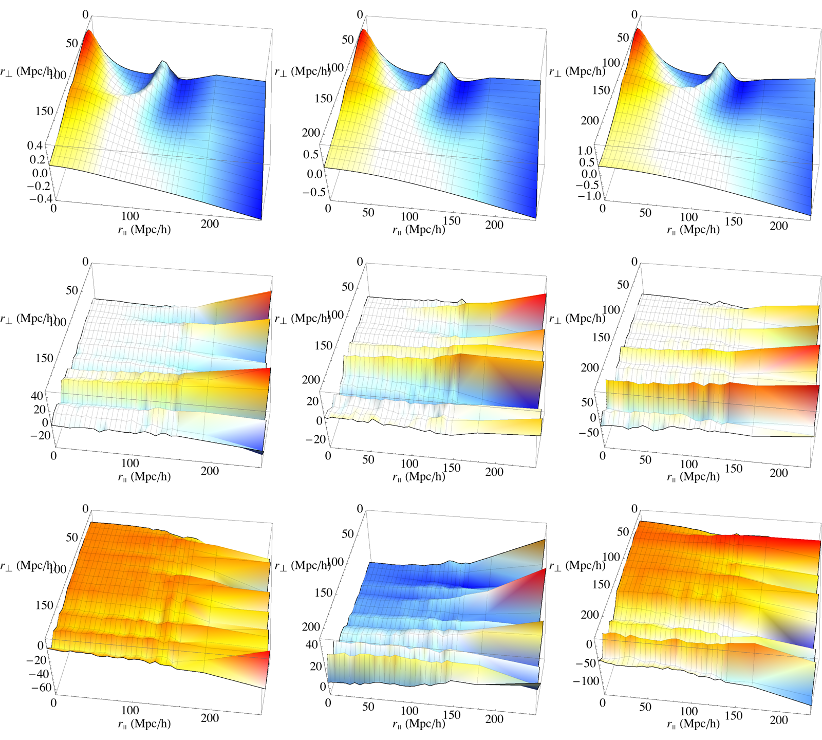
Figure 12 compares the data vectors for theory, simulated BOSS DR9 data, and actual BOSS DR9 data. The signal is visually obscured in the data by large-amplitude modes at fixed separation angles . However, these modes have negligible impact on our ability to measure BAO parameters since they have very small weights (by construction) in the covariance matrix (see Figure 13). The value of provides a rough measure of the overall (i.e., not BAO specific) signal to noise ratio of a sample. We find values of -8.5 and -8.3 for data and mocks, respectively, with , which indicates that the errors in our simulated data are about 30% larger than in real data. The signal to noise ratio is largest at , with errors about 40% larger at and three times larger at .
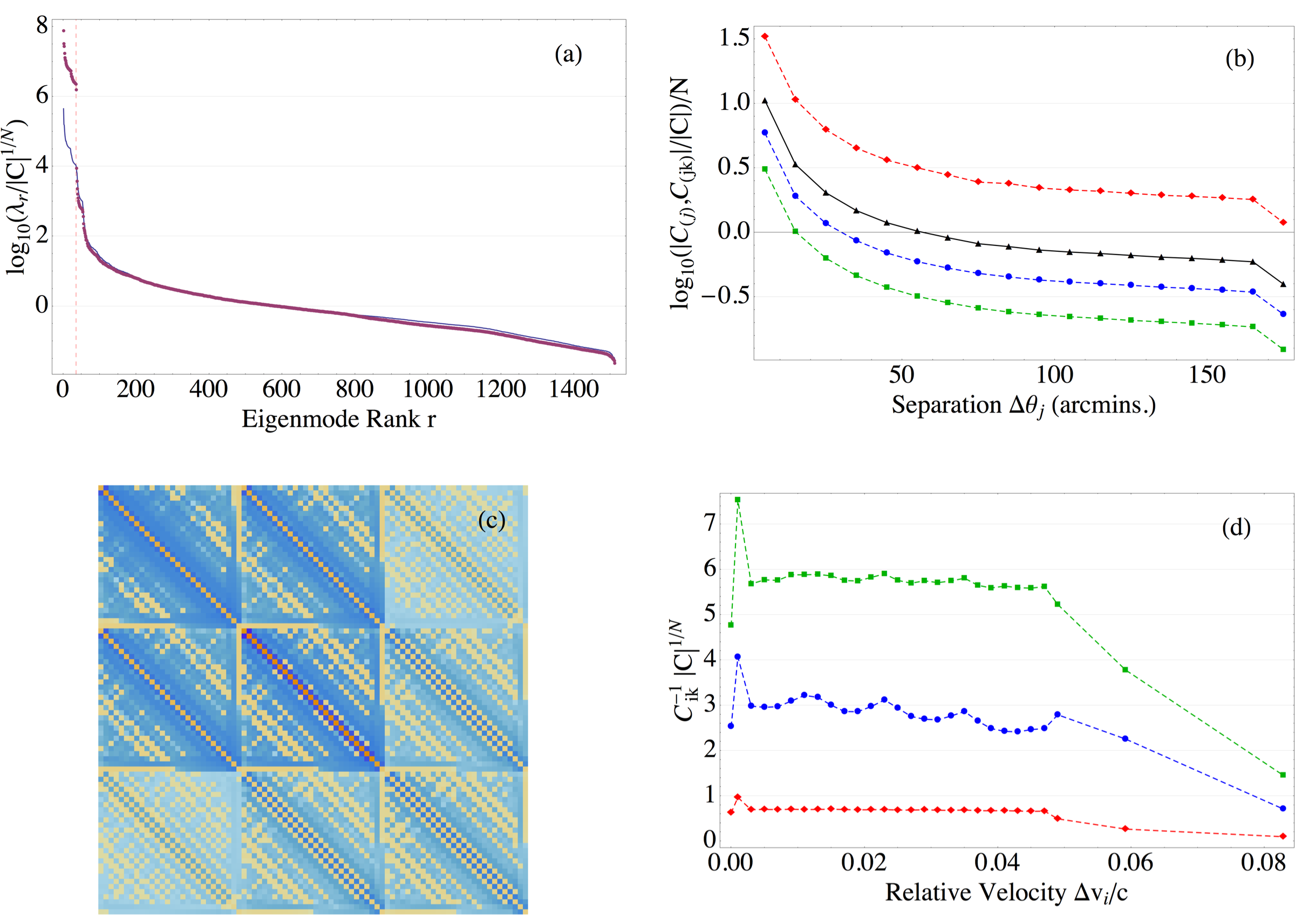
Figure 13 shows the structure of our covariance estimates, which is essentially the same for simulation and data after accounting for the % normalization difference. The first 36 eigenmodes have artificially large eigenvalues (see Figure 13a) due to the template marginalization procedure described in ref. [29], which accounts for the largest-amplitude modes visible in Figure 12. We expect correlation function estimates to be uncorrelated between different separation angles and therefore impose this constraint on our estimated inverse covariance matrix reducing both and to a block diagonal form consisting of 18 sub-matrices, and , with dimensions . Each of these submatrices has the same structure, shown in Figure 13c for , but a different normalization, or , depending on its separation (solid curve in Figure 13b). Each of the three sub-matrices on the diagonal, corresponding to a fixed separation and redshift , also have the same structure with normalizations shown as the dashed curves in Figure 13b. Values of the inverse covariance along the diagonal are roughly independent of and only depend on via the factor , as plotted in Figure 13d where the decreasing values at large correspond to increasing errors due to limited statistics.
Our correlation function estimates are actually provided as a set of quasi-independent data vectors and covariance matrices , corresponding to angular partition of the BOSS survey footprint into individual observing plates [29]. For fits to DR9, we have plates. We perform a weighted combination of observations, assumed to be independent, to obtain the final and used for fitting
| (3.5) |
The effective signal to noise ratio of individual observations spans about an order of magnitude (see Figure 14) due to varying observing conditions, so it is important that observations are correctly weighted in the combination. However, an overall normalization error in the estimated covariances still leads to a correctly weighted combination, even if the individual have different structures.
3.2 Internal Covariance Tests and Refinement
We exploit the large number of observations available to perform some internal cross checks on the individual and obtain improved estimates, as described below. First, we compare each observation to the combined observations using the chi-square statistic
| (3.6) |
where is the expected covariance of
| (3.7) |
and we have assumed that each is a Gaussian realization of some common true correlation function with additional noise sampled from
| (3.8) |
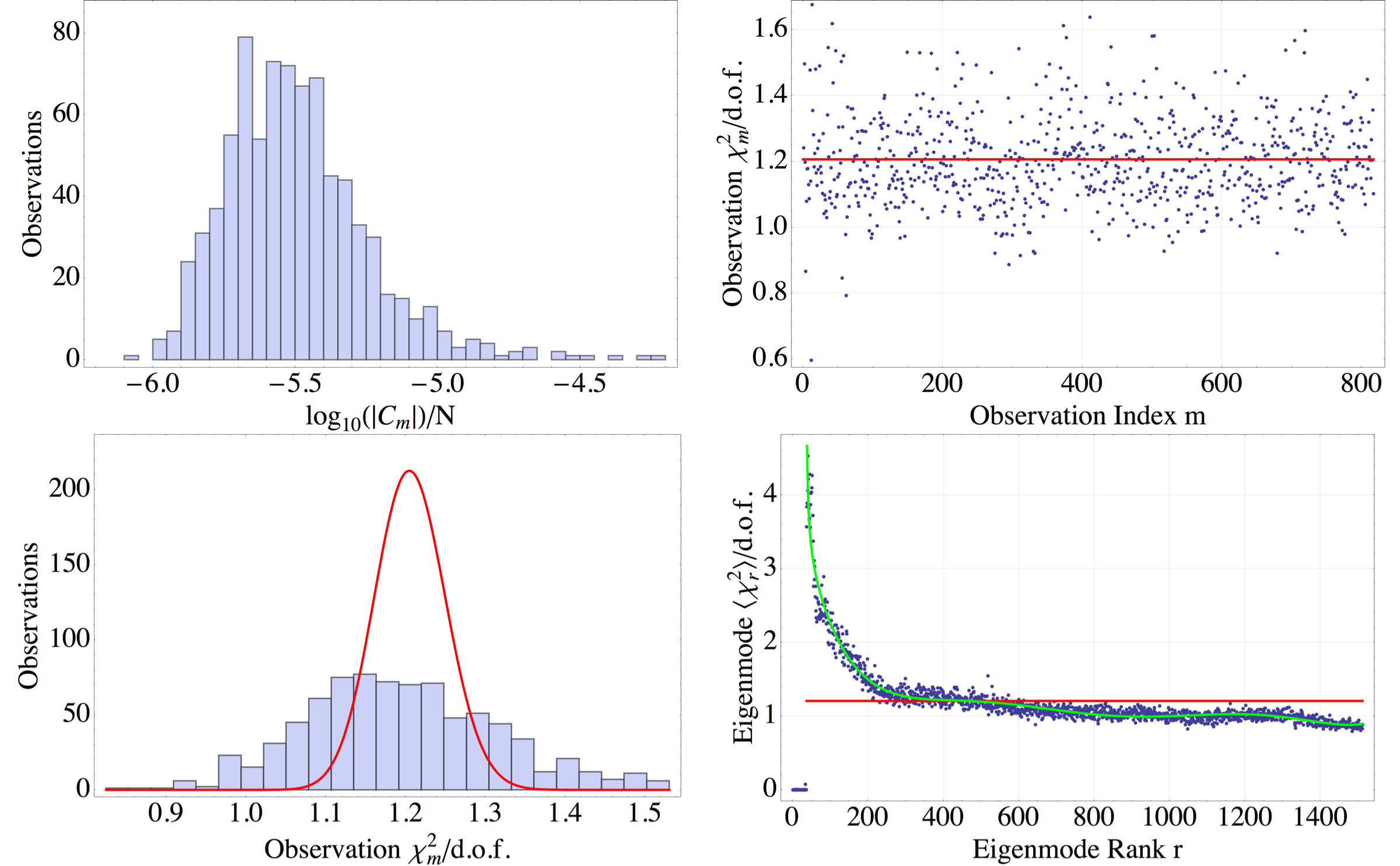
Figure 14 shows that, on average, our covariance estimates underestimate the actual variance seen in the data vectors by about 20%, but that this factor is independent of when the observation was taken. We then search for a correlation between the degree of underestimation and the amount of predicted variance by diagonalizing each
| (3.9) |
where is a diagonal matrix of the eigenvalues ranked in increasing size (larger predicted variance)
| (3.10) |
and is a matrix whose columns are the corresponding eigenvectors of . We can then rewrite as
| (3.11) |
where
| (3.12) |
and are the components of in the eigenvector basis for
| (3.13) |
Each should be chi-square distributed with one degree of freedom (if our assumptions of Gaussianity are valid) so we use their mean over the observations as a function of eigenvalue rank
| (3.14) |
to provide another internal test, where we expect for an eigenmode whose variance is correctly estimated. The results show (see Figure 14) that most of the 20% underestimation is due to the first eigenmodes with the largest predicted variances (but not including the 36 modes with artificially large variance mentioned above, which appear here with very small values of ).
We can partially correct for the deviations with eigenvalue rank shown in Figure 14 by independently rescaling each eigenmode of by . This procedure is not exact, however, since is derived from rather than (but we always have ) and because each generally has different eigenvectors (but we expect similar eigenvectors since the differ primarily in their normalizations). The results of this rescaling procedure are shown in Figure 15 and demonstrate that all eigenmodes now have internally consistent fluctuations and covariance estimates . Two caveats to this procedure are that we do not rescale the 36 previously marginalized modes and that we impose the expected block-diagonal structure on the rescaled , eliminating any off-diagonal contributions introduced by numerical round-off errors. Note that the distribution of the statistic has improved somewhat, compared with the Gaussian expectation, after rescaling. Finally, we combine the rescaled using eqn. (3.5) to obtain the final and used for the fits described below (and in Figs. 12 and 13).

We use bootstrap sampling in two different ways in our analysis. First, we boostrap our 817 estimates of the data vector to obtain an estimate of their combined covariance that is independent of the , as a cross-check of our combination using eqn. (3.5). With and , This approach is only feasible because of the block-diagonal structure of : we effectively bootstrap the elements of each block independently using 817 sub-vectors of length 84. We compare fit results obtained with the calculated combination and the corresponding bootstrap estimate of to check the validity of our calculated .
The second type of bootstrap analysis we perform is to fit a large number of bootstrap samples and then compare the resulting distributions of best-fit parameter values with the parabolic errors calculated from the likelihood surface of the combined fit using and . To the extent that the errors in our fit parameters are not Gaussian, we expect some discrepancy and then prefer the bootstrap estimates. Since our observations span an order of magnitude in weights , a sampling with replacement generally yields a set of observations whose combined covariance does not match the combined covariance of all observations. Therefore, some care is required in assigning the total covariance used to fit each bootstrap sample since, although we ignore the resulting fit errors, we still require a correct relative weighting over the physical coordinate grid in eqn. (3.4).
We generalize the combination method of eqn. (3.5) for bootstrap sampling to
| (3.15) |
where is the number of repetitions of observation and is the bootstrap sample size (usually ). The resulting is not the covariance of since it incorrectly reduces the variance for double-counted observations. Instead, the correct covariance to use is
| (3.16) |
with
| (3.17) |
Note that eqn. (3.15) reduces to eqn. (3.5) when each , so that each sample is either not used, (if ), or used exactly once, . In the limit that all are identical, we find
| (3.18) |
where is the chi-squared that would be obtained using instead of in eqn. (3.4). In the usual case of , we find a ratio .
Before performing fits, we generally apply some final cuts to select a subset of the three-dimensional grid points. Cuts can either be in physical or (using the fiducial cosmology) comoving coordinates. We implement cuts by first combining all observations using eqn. (3.5), without cuts, and then eliminating elements from the final data vector , as well as the corresponding rows and columns of . Note that the resulting is different from what we would have obtained by eliminating rows and columns from directly. Our nominal final cuts on physical coordinates are and arcminutes. We also cut on the co-moving separation Mpc/h. After all final cuts, the size of our data vector is reduced from to 341 () + 310 () + 290 () = 941.
4 Results
In this section, we present results related to the fitting methods and what they reveal about the BOSS DR9 Lyman- forest sample. Cosmological fit results derived from the same sample are presented in the companion paper ref. [29].
4.1 Parameter Sensitivities
In order to quantify and visualize how a dataset constrains each parameter , it is instructive to plot the vector
| (4.1) |
where is the partial derivative of the theory prediction at some point in parameter space , and represents the Hadamard (entrywise) product. The sum of the resulting components is the Fisher information for parameter [36] that specifies the expected maximum-likelihood error (in an ensemble-average sense) when all other parameter values are known
| (4.2) |
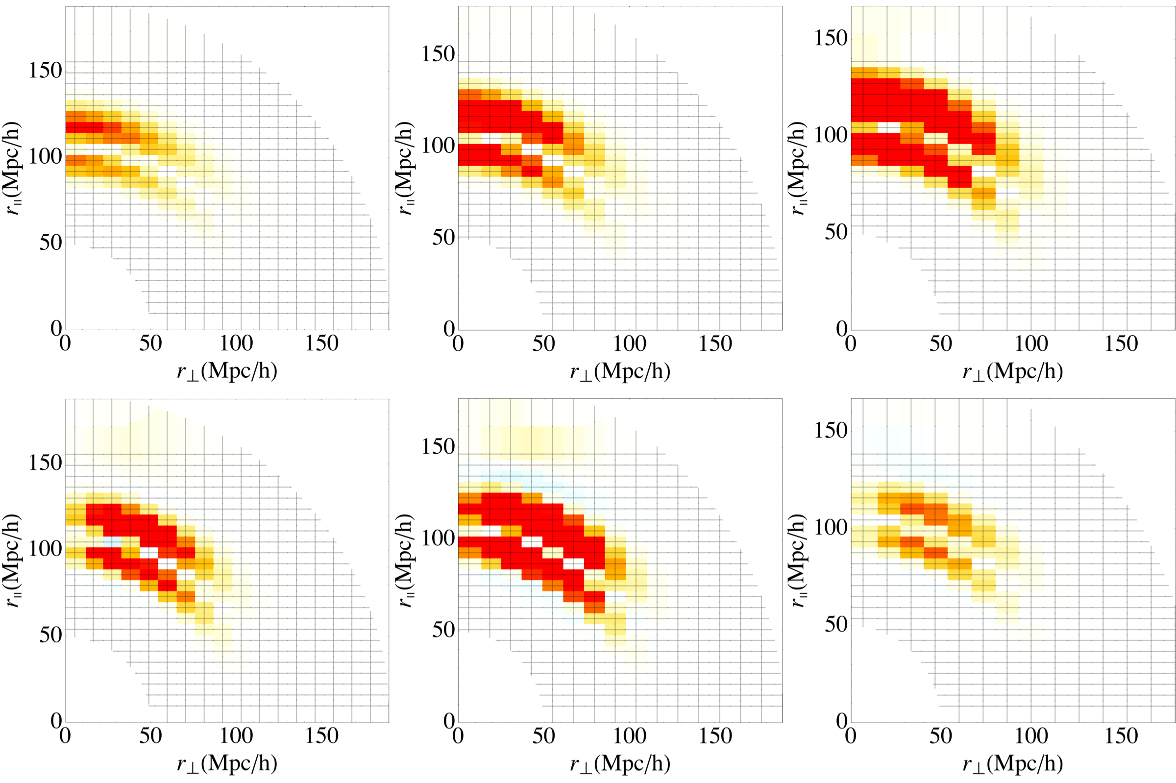
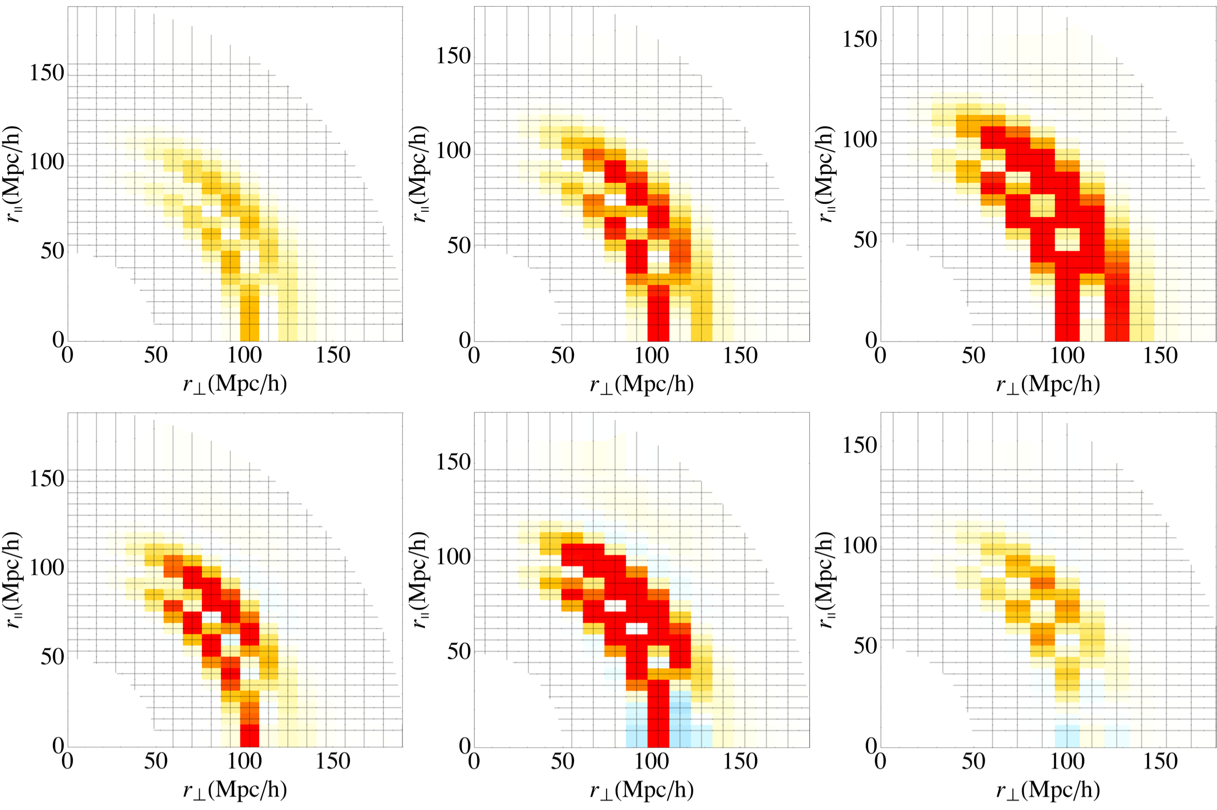
The theory derivatives encode the parameter sensitivity inherent to the model while the covariance encodes the performance of a particular analysis method. The quantity is plotted for our baseline fit to BOSS DR9 for the isotropic scale parameter in Figure 16 and for the anisotropic scale parameters in Figures 17 () and 18 ().
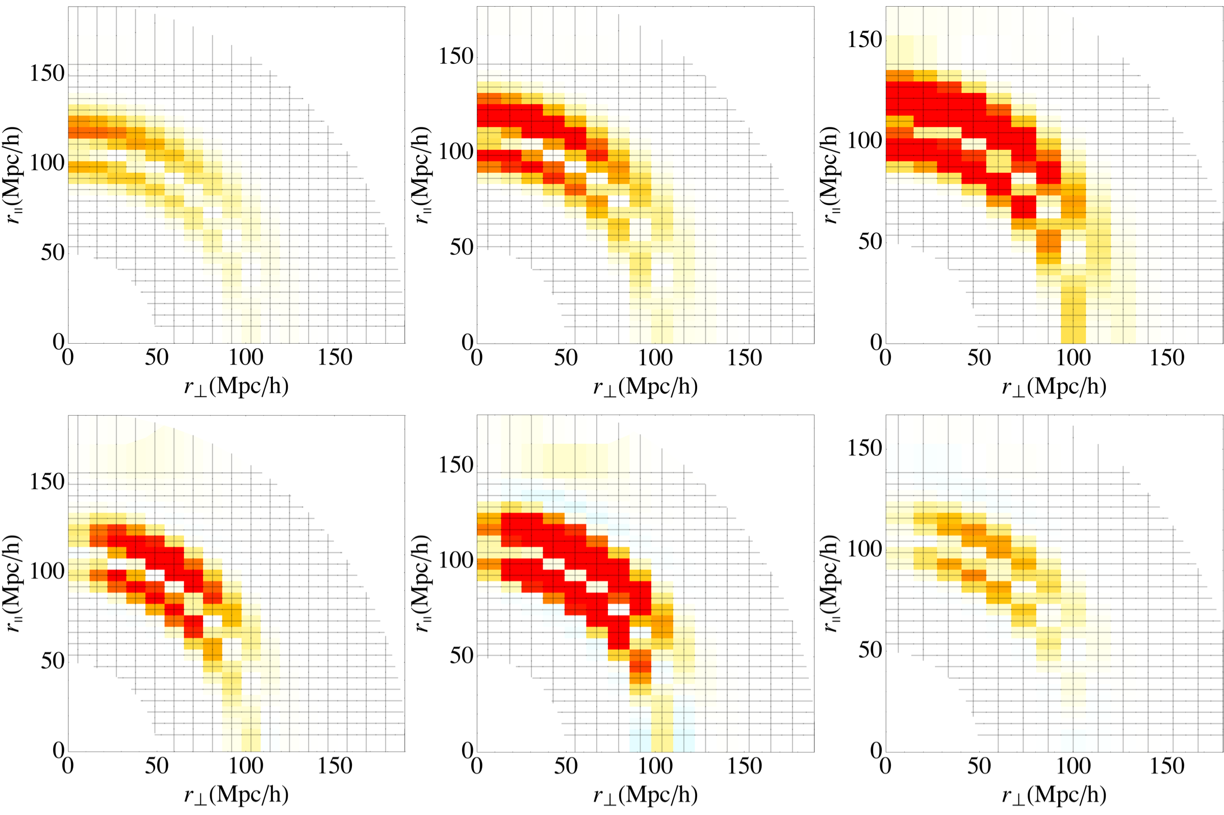
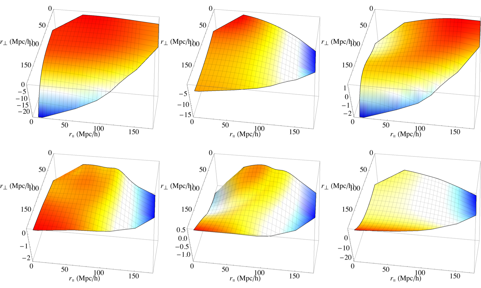
The top row of Figure 16 uses to isolate the intrinsic model sensitivity, resulting in a Fisher error prediction of , with inverse-variance contributions of 12%, 28%, 60% from 2, 2.5, 3, respectively, due to the observed large increase in tracer bias with redshift governed by the parameter . Information on the BAO scale comes predominantly from the forward direction due to the large observed value of the redshift-distortion parameter , and is concentrated on two rings in co-moving separation on either side of the BAO peak, where the theory is most sensitive to the peak position. When the combined covariance is taken into account, the Fisher error prediction increases slightly to , and the region of peak sensitivity moves from to , mostly due to the trend shown in Figure 13(b). Intermediate redshifts now dominate the statistical power due to the distribution of forest pixel redshifts, with inverse-variance contributions of 29%, 61%, 10% from 2, 2.5, 3, respectively.
When floating the scales parallel and perpendicular to the line of sight, the Fisher predicted errors are 0.024 (0.021) and 0.050 (0.047) for the combined analysis covariance (using ). Note that our actual covariance actually reduces the expected error on , relative to , because of the decreasing errors with separation angle shown in Figure 13b. The peak predicted sensitivities are for and for .
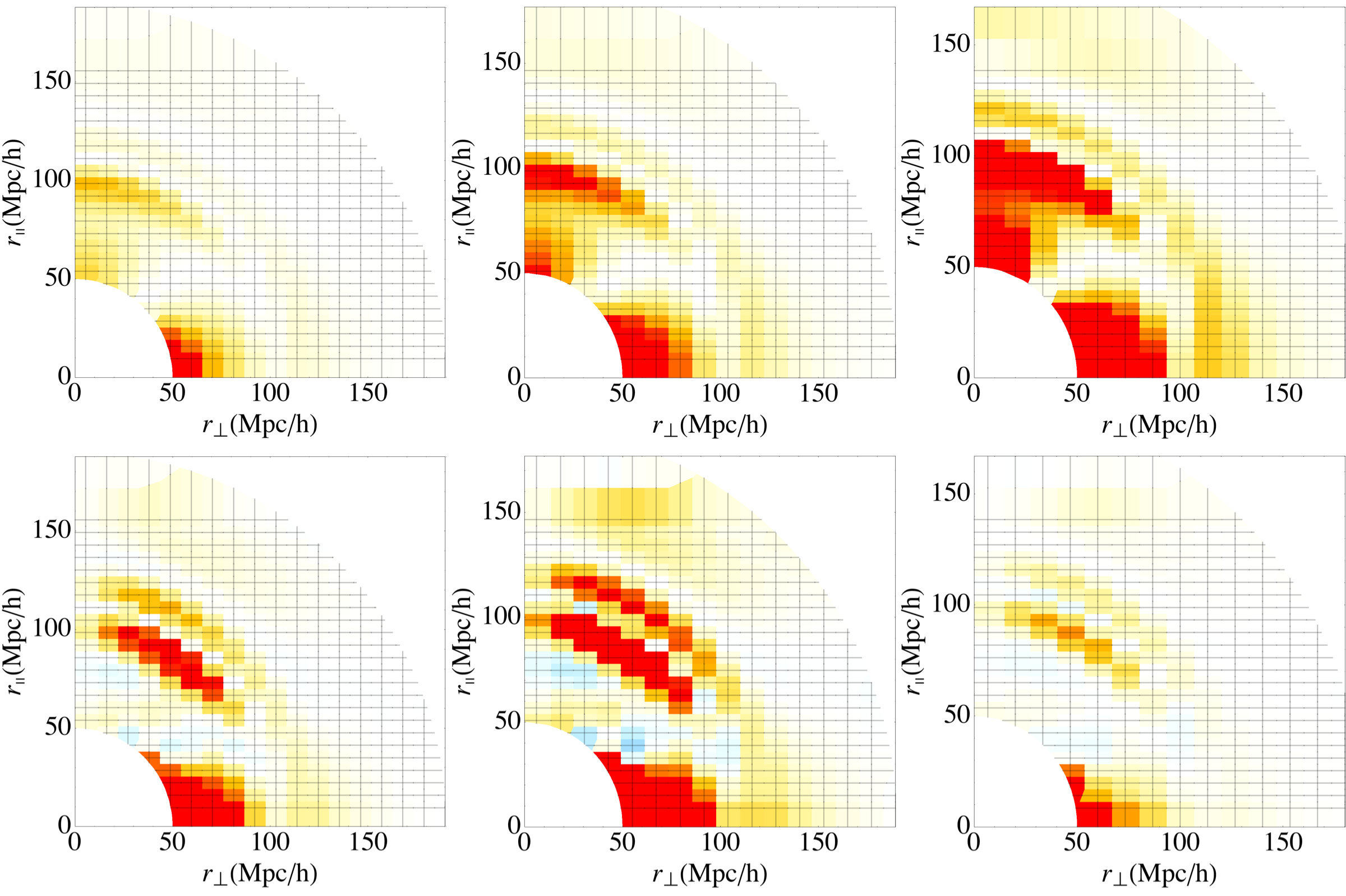
The results above were obtained with in eqn. (2.34), so that scale factors are applied only to the peak position and not the cosmological broadband. If, instead, we use , the resulting Fisher components for an isotropic fit are shown in Figure 19, resulting in a smaller predicted error of (0.013) for the combined analysis covariance (using ). Comparing with Figure 16, we conclude that a fit using coupled transforms obtains a smaller error (when all other parameter values are fixed) by using information outside of the peak region. However, this benefit is offset by a larger dependence on the broadband distortion model, and the final errors are comparable when marginalizing over distortion parameters. For fits to DR9, we prefer to localize the BAO scale measurement to the peak region and minimize our dependence on the distortion model. With larger data samples and improved analyses, we expect to have better control of distortion effects and this choice should be revisited.
4.2 Data Reductions
The 1512 fit inputs already represent a substantial reduction of data from the millions of Lyman- forest pixel pairs from which they are derived, while preserving essentially all of the cosmologically relevant information. We can take this process one step further using the interpolated models of Section 2.4 to reduce down to estimates of multipoles of the correlation function or power spectrum. There are two main challenges in this process: first, the input has large correlated errors that will propagate through and, second, the input is expected to include some broadband distortion that prevents direct comparison of reduced data with theory. Therefore, we first test our data reductions on a mock dataset based on our fiducial cosmology and with the same covariance as data, but no distortion, and then compare these to the corresponding results obtained from data.
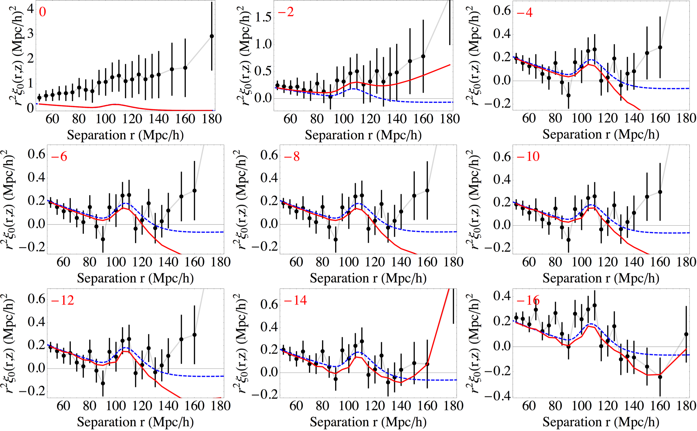
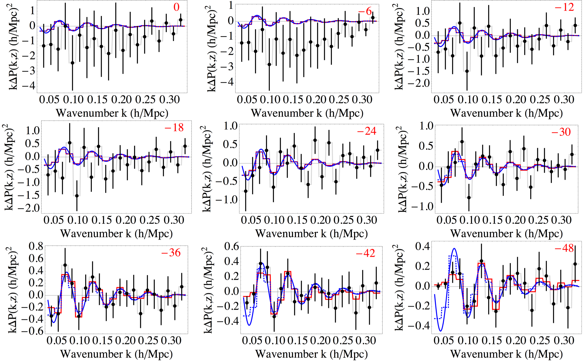
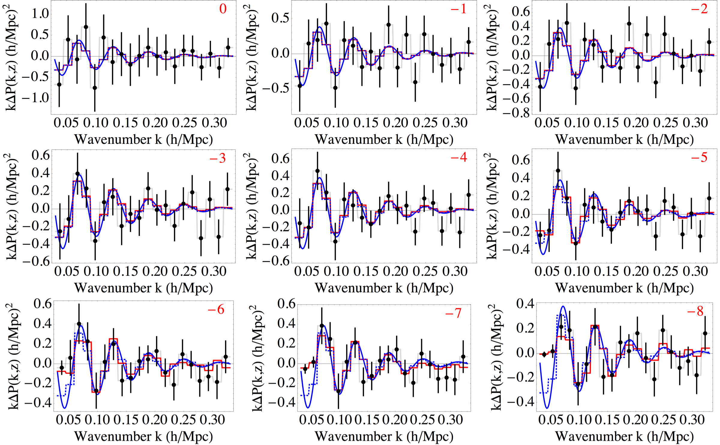
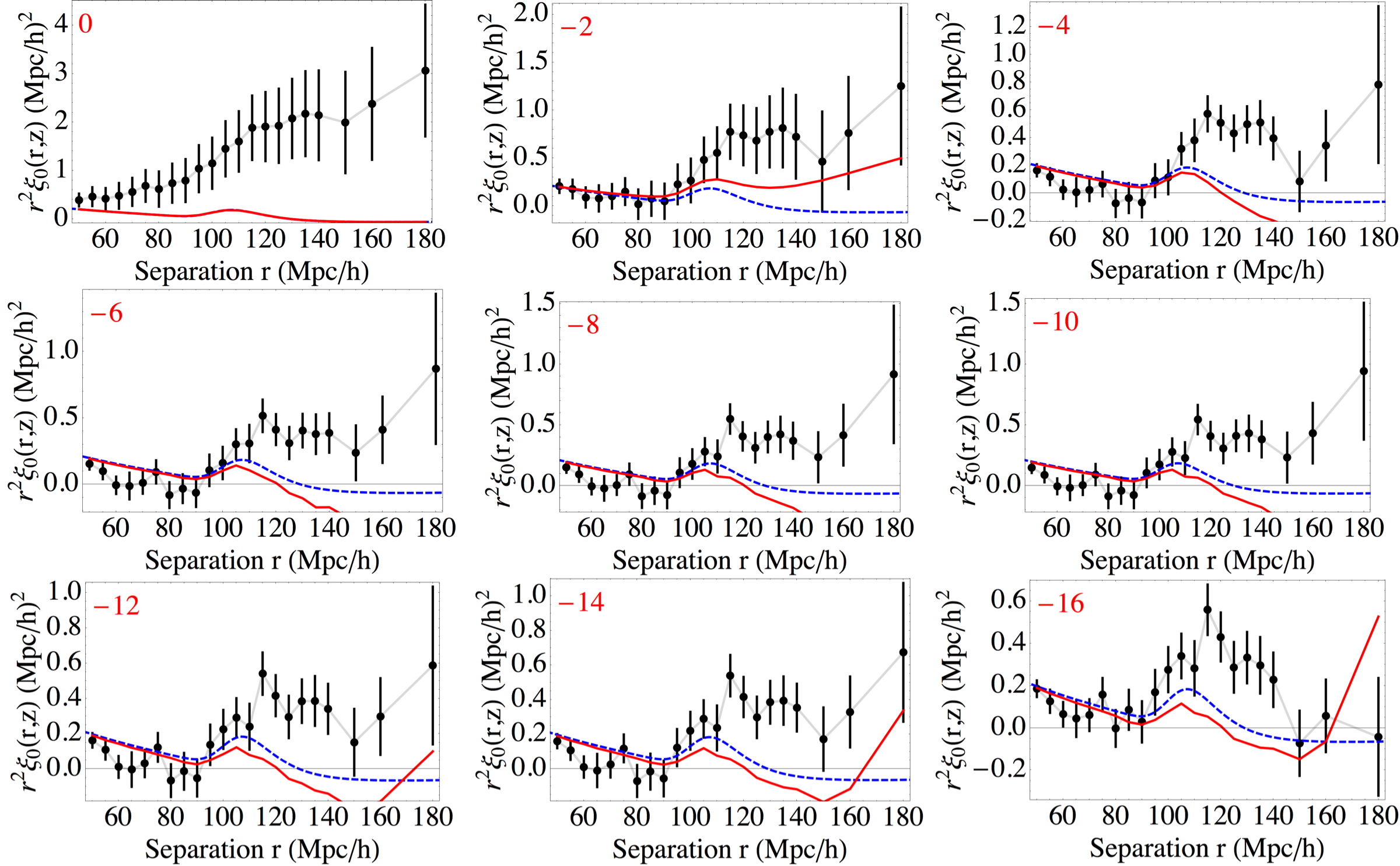
We use three different types of model-independent fits for data reduction. The first fit estimates the -weighted correlation function multipoles at as a linear interpolation between 22 co-moving separations (5–140 in steps of 5, followed by 150, 160, and 180 Mpc/h) using eqn. (2.77), for a total reduction from 1512 to 66 values. The second fit estimates the -weighted power spectrum multipoles at as a set 20 of equally spaced band powers covering –0.33 h/Mpc with h/Mpc, using eqn. (2.80) with 0-th order B-splines, for a total reduction from 1512 to 60 values. Our final model assumes that the multipoles are identical except for the normalization factor eqn. (2.78), which is expected to be a good approximation if broadband distortion is either small or else experiences similar redshift-space distortion as the linear theory, and results in 20 final values. In all of our data reduction fits, we assume , , and , and our results are normalized using . We have made the results of these data reductions publicly available (see Appendix A).
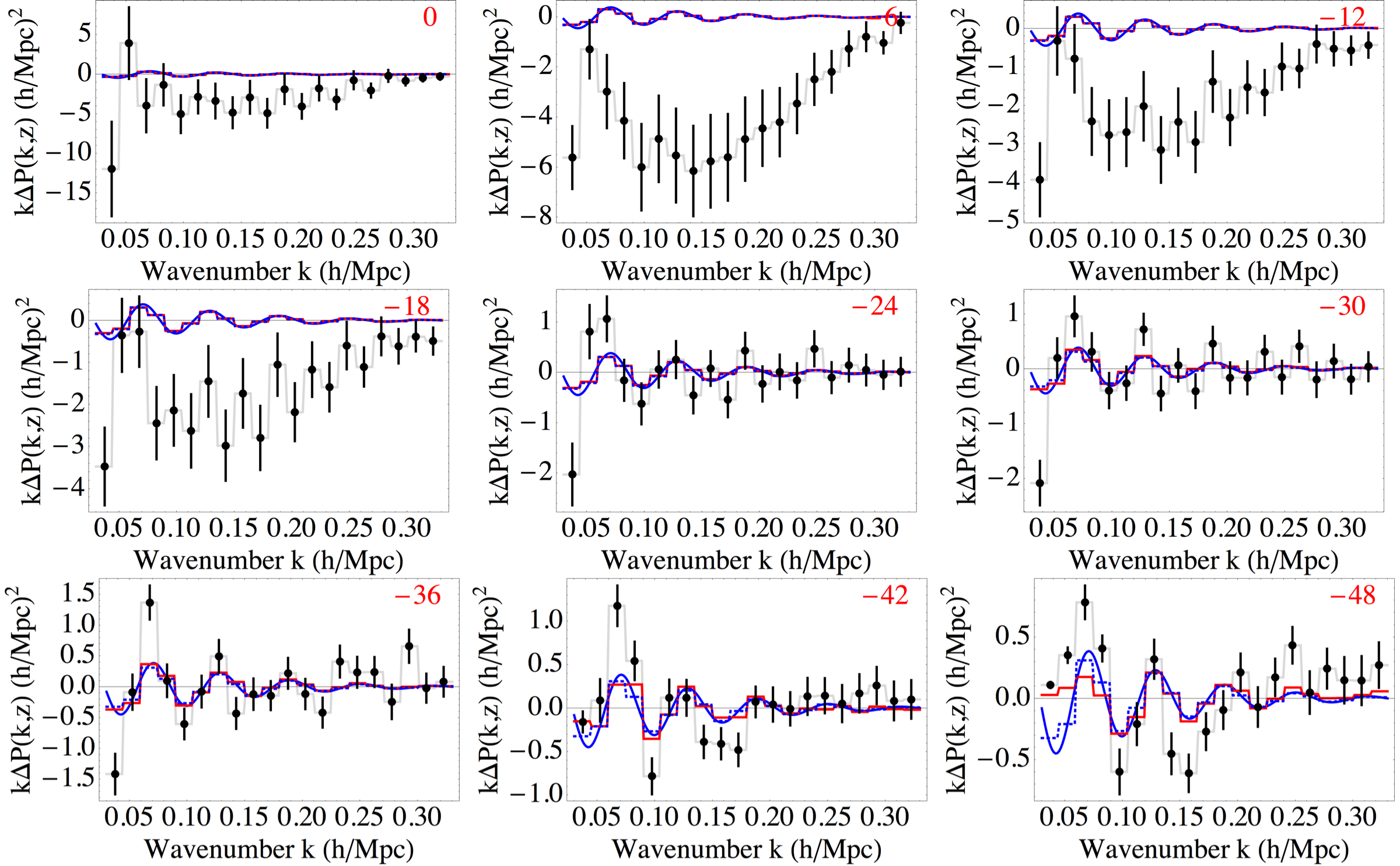
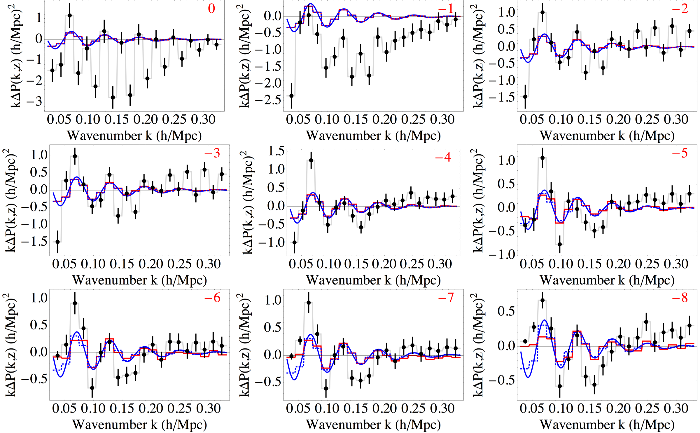
Figure 20 shows the ranked eigenvalues of the parameter covariance matrices for fits to data and the un-distorted mock dataset, and demonstrates that the data and mock have essentially the same parameter covariance structure. For the purposes of visualization, it is helpful to project out the largest eigenmodes of the parameter covariance matrix, which eliminates the largest sources of correlated errors but can also introduce a projection distortion of the reduced data (in addition to any distortion from the analysis method). The optimum number of modes to project out is a balance between minimizing correlated errors and minimizing projection distortion effects. Figs. 21–23 show the results of projecting different numbers of eigenvalues on the monopole of our un-distorted mock, and allows us to identify an appropriate number of modes to filter for each data reduction fit: -14, -36, and -6, respectively.

Figs. 24–26 show the same reductions as Figs. 21–23, but applied to data instead of un-distorted mocks. Comparing these, we conclude that the projection distortion effects are similar for each reduction. We also note that the analysis introduces significant broadband distortion that is most apparent (especially with the weighting) as a broad excess above 110 Mpc/h in the correlation-function monopole (Figure 21 with 14 modes projected out). Since this broadband distortion corresponds to low- modes, the data reductions are relatively immune to it. Instead, they show an enhancement of the BAO oscillation signal relative to the fiducial model. Further study with additional data is needed to determine if this excess is a fortunate statistical fluctuation or if perhaps the signal is larger than expected.
5 Discussion
In this paper we have described a near-optimal method for fitting correlations observed in the Lyman- forest of high-redshift quasars to measure the properties of the baryon acoustic oscillation feature. We also explore the properties of the BOSS DR9 correlation estimates described in ref. [29], and provide the code and input files necessary to reproduce our main results.
Comparing with the Lyman- fitting methods used in ref. [24], where correlations are modeled in the monopole and quadrupole at a single mean redshift, we have developed a fully three-dimensional fitting technique and included the effects of anisotropic non-linear broadening. These developments do not yield a significant improvement in the cosmological constraints that are possible with DR9, but provide more flexibility to study and quantify systematics and allow direct study the redshift evolution of parameters such as and , and to accurately determine the effective redshift of our cosmological constraints.
The challenge of a three-dimensional analysis is that the resulting large covariance matrix is difficult to estimate and validate, especially with the limited number of mocks available for the DR9 Lyman- forest. However, we have developed a novel method for internally testing and refining our large covariance matrix, as described in Section 3.2. The resulting covariance matrix still has large correlations that visually obscure the BAO signal but have little impact on our ability to measure its properties. We describe data reductions that retain most of the cosmologically relevant information and show how the expected features are visually revealed when large eigenmodes are projected out.
In building models suitable for a three-dimensional analysis, we find that care is needed to isolate the BAO feature in the correlation function and describe an alternative to the “no-wiggles” approach of ref. [34] that is better suited for this purpose. When considering the line of sight () and transverse () scale factors independently, we find that a first-order treatment is numerically inaccurate near the BAO peak, and identify the important second-order terms. We introduce anisotropic non-linear broadening using an approximation that is valid for a large range of . We also use a highly flexible parametrization of both multiplicative and additive broadband distortions to accomodate the expected systematics of the correlation-function estimates due to effects such as a biased continuum estimate. Finally, we demonstrate that information on the BAO feature in the Lyman- forest arises primarily along the line of sight, as expected due to the large redshift-space distortion, but that the contributions from and can still be independently measured.
The first measurements of baryon acoustic oscillations in the Lyman- forest [24, 29] provide a new confirmation of our basic picture of cosmological evolution dominated by dark energy, but do not yet significantly constrain the parameters of the simplest cosmological models. With the SDSS-III high-redshift quasar sample expected to triple the DR9 statistics over the next 18 months, that situation is likely to change and will require near-optimal fitting methods and a flexible framework for careful study of systematics.
Acknowledgments
Funding for SDSS-III has been provided by the Alfred P. Sloan Foundation, the Participating Institutions, the National Science Foundation, and the U.S. Department of Energy Office of Science. The SDSS-III web site is http://www.sdss3.org/.
SDSS-III is managed by the Astrophysical Research Consortium for the Participating Institutions of the SDSS-III Collaboration including the University of Arizona, the Brazilian Participation Group, Brookhaven National Laboratory, University of Cambridge, Carnegie Mellon University, University of Florida, the French Participation Group, the German Participation Group, Harvard University, the Instituto de Astrofisica de Canarias, the Michigan State/Notre Dame/JINA Participation Group, Johns Hopkins University, Lawrence Berkeley National Laboratory, Max Planck Institute for Astrophysics, Max Planck Institute for Extraterrestrial Physics, New Mexico State University, New York University, Ohio State University, Pennsylvania State University, University of Portsmouth, Princeton University, the Spanish Participation Group, University of Tokyo, University of Utah, Vanderbilt University, University of Virginia, University of Washington, and Yale University.
References
- [1] A. G. Riess, A. V. Filippenko, P. Challis, A. Clocchiatti, A. Diercks, P. M. Garnavich, R. L. Gilliland, C. J. Hogan, S. Jha, R. P. Kirshner, B. Leibundgut, M. M. Phillips, D. Reiss, B. P. Schmidt, R. A. Schommer, R. C. Smith, J. Spyromilio, C. Stubbs, N. B. Suntzeff, and J. Tonry, Observational Evidence from Supernovae for an Accelerating Universe and a Cosmological Constant, AJ 116 (Sept., 1998) 1009–1038, [astro-ph/].
- [2] S. Perlmutter, G. Aldering, G. Goldhaber, R. A. Knop, P. Nugent, P. G. Castro, S. Deustua, S. Fabbro, A. Goobar, D. E. Groom, I. M. Hook, A. G. Kim, M. Y. Kim, J. C. Lee, N. J. Nunes, R. Pain, C. R. Pennypacker, R. Quimby, C. Lidman, R. S. Ellis, M. Irwin, R. G. McMahon, P. Ruiz-Lapuente, N. Walton, B. Schaefer, B. J. Boyle, A. V. Filippenko, T. Matheson, A. S. Fruchter, N. Panagia, H. J. M. Newberg, W. J. Couch, and The Supernova Cosmology Project, Measurements of Omega and Lambda from 42 High-Redshift Supernovae, ApJ 517 (June, 1999) 565–586, [astro-ph/].
- [3] D. H. Weinberg, M. J. Mortonson, D. J. Eisenstein, C. Hirata, A. G. Riess, and E. Rozo, Observational Probes of Cosmic Acceleration, ArXiv e-prints (Jan., 2012) [arXiv:1201.2434].
- [4] E. Komatsu, K. M. Smith, J. Dunkley, C. L. Bennett, B. Gold, G. Hinshaw, N. Jarosik, D. Larson, M. R. Nolta, L. Page, D. N. Spergel, M. Halpern, R. S. Hill, A. Kogut, M. Limon, S. S. Meyer, N. Odegard, G. S. Tucker, J. L. Weiland, E. Wollack, and E. L. Wright, Seven-year Wilkinson Microwave Anisotropy Probe (WMAP) Observations: Cosmological Interpretation, ApJS 192 (Feb., 2011) 18, [arXiv:1001.4538].
- [5] e. Hinshaw, G. F., Nine-year Wilkinson Microwave Anisotropy Probe (WMAP) Observations: Cosmological Results, ApJS (2012) [arXiv:1212.5226].
- [6] W. J. Percival, C. M. Baugh, J. Bland-Hawthorn, T. Bridges, R. Cannon, S. Cole, M. Colless, C. Collins, W. Couch, G. Dalton, R. De Propris, S. P. Driver, G. Efstathiou, R. S. Ellis, C. S. Frenk, K. Glazebrook, C. Jackson, O. Lahav, I. Lewis, S. Lumsden, S. Maddox, S. Moody, P. Norberg, J. A. Peacock, B. A. Peterson, W. Sutherland, and K. Taylor, The 2dF Galaxy Redshift Survey: the power spectrum and the matter content of the Universe, MNRAS 327 (Nov., 2001) 1297–1306.
- [7] C. J. Miller, R. C. Nichol, and D. J. Batuski, Possible Detection of Baryonic Fluctuations in the Large-Scale Structure Power Spectrum, ApJ 555 (July, 2001) 68–73, [astro-ph/].
- [8] D. J. Eisenstein, I. Zehavi, D. W. Hogg, R. Scoccimarro, M. R. Blanton, R. C. Nichol, R. Scranton, H.-J. Seo, M. Tegmark, Z. Zheng, S. F. Anderson, J. Annis, N. Bahcall, J. Brinkmann, S. Burles, F. J. Castander, A. Connolly, I. Csabai, M. Doi, M. Fukugita, J. A. Frieman, K. Glazebrook, J. E. Gunn, J. S. Hendry, G. Hennessy, Z. Ivezić, S. Kent, G. R. Knapp, H. Lin, Y.-S. Loh, R. H. Lupton, B. Margon, T. A. McKay, A. Meiksin, J. A. Munn, A. Pope, M. W. Richmond, D. Schlegel, D. P. Schneider, K. Shimasaku, C. Stoughton, M. A. Strauss, M. SubbaRao, A. S. Szalay, I. Szapudi, D. L. Tucker, B. Yanny, and D. G. York, Detection of the Baryon Acoustic Peak in the Large-Scale Correlation Function of SDSS Luminous Red Galaxies, ApJ 633 (Nov., 2005) 560–574.
- [9] S. Cole, W. J. Percival, J. A. Peacock, P. Norberg, C. M. Baugh, C. S. Frenk, I. Baldry, J. Bland-Hawthorn, T. Bridges, R. Cannon, M. Colless, C. Collins, W. Couch, N. J. G. Cross, G. Dalton, V. R. Eke, R. De Propris, S. P. Driver, G. Efstathiou, R. S. Ellis, K. Glazebrook, C. Jackson, A. Jenkins, O. Lahav, I. Lewis, S. Lumsden, S. Maddox, D. Madgwick, B. A. Peterson, W. Sutherland, and K. Taylor, The 2dF Galaxy Redshift Survey: power-spectrum analysis of the final data set and cosmological implications, MNRAS 362 (Sept., 2005) 505–534, [astro-ph/].
- [10] G. Hütsi, Power spectrum of the SDSS luminous red galaxies: constraints on cosmological parameters, A&A 459 (Nov., 2006) 375–389, [astro-ph/].
- [11] N. Padmanabhan, D. J. Schlegel, U. Seljak, A. Makarov, N. A. Bahcall, M. R. Blanton, J. Brinkmann, D. J. Eisenstein, D. P. Finkbeiner, J. E. Gunn, D. W. Hogg, Ž. Ivezić, G. R. Knapp, J. Loveday, R. H. Lupton, R. C. Nichol, D. P. Schneider, M. A. Strauss, M. Tegmark, and D. G. York, The clustering of luminous red galaxies in the Sloan Digital Sky Survey imaging data, MNRAS 378 (July, 2007) 852–872, [astro-ph/].
- [12] C. Blake, A. Collister, S. Bridle, and O. Lahav, Cosmological baryonic and matter densities from 600000 SDSS luminous red galaxies with photometric redshifts, MNRAS 374 (Feb., 2007) 1527–1548, [astro-ph/].
- [13] W. J. Percival, S. Cole, D. J. Eisenstein, R. C. Nichol, J. A. Peacock, A. C. Pope, and A. S. Szalay, Measuring the Baryon Acoustic Oscillation scale using the Sloan Digital Sky Survey and 2dF Galaxy Redshift Survey, MNRAS 381 (Nov., 2007) 1053–1066, [arXiv:0705.3323].
- [14] T. Okumura, T. Matsubara, D. J. Eisenstein, I. Kayo, C. Hikage, A. S. Szalay, and D. P. Schneider, Large-Scale Anisotropic Correlation Function of SDSS Luminous Red Galaxies, ApJ 676 (Apr., 2008) 889–898, [arXiv:0711.3640].
- [15] E. Gaztañaga, A. Cabré, and L. Hui, Clustering of luminous red galaxies - IV. Baryon acoustic peak in the line-of-sight direction and a direct measurement of H(z), MNRAS 399 (Nov., 2009) 1663–1680, [arXiv:0807.3551].
- [16] E. A. Kazin, M. R. Blanton, R. Scoccimarro, C. K. McBride, A. A. Berlind, N. A. Bahcall, J. Brinkmann, P. Czarapata, J. A. Frieman, S. M. Kent, D. P. Schneider, and A. S. Szalay, The Baryonic Acoustic Feature and Large-Scale Clustering in the Sloan Digital Sky Survey Luminous Red Galaxy Sample, ApJ 710 (Feb., 2010) 1444–1461, [arXiv:0908.2598].
- [17] W. J. Percival, B. A. Reid, D. J. Eisenstein, N. A. Bahcall, T. Budavari, J. A. Frieman, M. Fukugita, J. E. Gunn, Ž. Ivezić, G. R. Knapp, R. G. Kron, J. Loveday, R. H. Lupton, T. A. McKay, A. Meiksin, R. C. Nichol, A. C. Pope, D. J. Schlegel, D. P. Schneider, D. N. Spergel, C. Stoughton, M. A. Strauss, A. S. Szalay, M. Tegmark, M. S. Vogeley, D. H. Weinberg, D. G. York, and I. Zehavi, Baryon acoustic oscillations in the Sloan Digital Sky Survey Data Release 7 galaxy sample, MNRAS 401 (Feb., 2010) 2148–2168, [arXiv:0907.1660].
- [18] B. A. Reid, W. J. Percival, D. J. Eisenstein, L. Verde, D. N. Spergel, R. A. Skibba, N. A. Bahcall, T. Budavari, J. A. Frieman, M. Fukugita, J. R. Gott, J. E. Gunn, Ž. Ivezić, G. R. Knapp, R. G. Kron, R. H. Lupton, T. A. McKay, A. Meiksin, R. C. Nichol, A. C. Pope, D. J. Schlegel, D. P. Schneider, C. Stoughton, M. A. Strauss, A. S. Szalay, M. Tegmark, M. S. Vogeley, D. H. Weinberg, D. G. York, and I. Zehavi, Cosmological constraints from the clustering of the Sloan Digital Sky Survey DR7 luminous red galaxies, MNRAS 404 (May, 2010) 60–85, [arXiv:0907.1659].
- [19] C. Blake, E. A. Kazin, F. Beutler, T. M. Davis, D. Parkinson, S. Brough, M. Colless, C. Contreras, W. Couch, S. Croom, D. Croton, M. J. Drinkwater, K. Forster, D. Gilbank, M. Gladders, K. Glazebrook, B. Jelliffe, R. J. Jurek, I.-H. Li, B. Madore, D. C. Martin, K. Pimbblet, G. B. Poole, M. Pracy, R. Sharp, E. Wisnioski, D. Woods, T. K. Wyder, and H. K. C. Yee, The WiggleZ Dark Energy Survey: mapping the distance-redshift relation with baryon acoustic oscillations, MNRAS 418 (Dec., 2011) 1707–1724, [arXiv:1108.2635].
- [20] F. Beutler, C. Blake, M. Colless, D. H. Jones, L. Staveley-Smith, L. Campbell, Q. Parker, W. Saunders, and F. Watson, The 6dF Galaxy Survey: baryon acoustic oscillations and the local Hubble constant, MNRAS 416 (Oct., 2011) 3017–3032, [arXiv:1106.3366].
- [21] H.-J. Seo, S. Ho, M. White, A. J. Cuesta, A. J. Ross, S. Saito, B. Reid, N. Padmanabhan, W. J. Percival, R. de Putter, D. J. Schlegel, D. J. Eisenstein, X. Xu, D. P. Schneider, R. Skibba, L. Verde, R. C. Nichol, D. Bizyaev, H. Brewington, J. Brinkmann, L. A. Nicolaci da Costa, J. R. Gott, III, E. Malanushenko, V. Malanushenko, D. Oravetz, N. Palanque-Delabrouille, K. Pan, F. Prada, N. P. Ross, A. Simmons, F. de Simoni, A. Shelden, S. Snedden, and I. Zehavi, Acoustic Scale from the Angular Power Spectra of SDSS-III DR8 Photometric Luminous Galaxies, ApJ 761 (Dec., 2012) 13, [arXiv:1201.2172].
- [22] N. Padmanabhan, X. Xu, D. J. Eisenstein, R. Scalzo, A. J. Cuesta, K. T. Mehta, and E. Kazin, A 2% Distance to z=0.35 by Reconstructing Baryon Acoustic Oscillations - I : Methods and Application to the Sloan Digital Sky Survey, ArXiv e-prints (Jan., 2012) [arXiv:1202.0090].
- [23] L. Anderson, E. Aubourg, S. Bailey, D. Bizyaev, M. Blanton, A. S. Bolton, J. Brinkmann, J. R. Brownstein, A. Burden, A. J. Cuesta, L. N. A. da Costa, K. S. Dawson, R. de Putter, D. J. Eisenstein, J. E. Gunn, H. Guo, J.-C. Hamilton, P. Harding, S. Ho, K. Honscheid, E. Kazin, D. Kirkby, J.-P. Kneib, A. Labatie, C. Loomis, R. H. Lupton, E. Malanushenko, V. Malanushenko, R. Mandelbaum, M. Manera, C. Maraston, C. K. McBride, K. T. Mehta, O. Mena, F. Montesano, D. Muna, R. C. Nichol, S. E. Nuza, M. D. Olmstead, D. Oravetz, N. Padmanabhan, N. Palanque-Delabrouille, K. Pan, J. Parejko, I. Paris, W. J. Percival, P. Petitjean, F. Prada, B. Reid, N. A. Roe, A. J. Ross, N. P. Ross, L. Samushia, A. G. Sanchez, D. J. S. D. P. Schneider, C. G. Scoccola, H.-J. Seo, E. S. Sheldon, A. Simmons, R. A. Skibba, M. A. Strauss, M. E. C. Swanson, D. Thomas, J. L. Tinker, R. Tojeiro, M. Vargas Magana, L. Verde, C. Wagner, D. A. Wake, B. A. Weaver, D. H. Weinberg, M. White, X. Xu, C. Yeche, I. Zehavi, and G.-B. Zhao, The clustering of galaxies in the SDSS-III Baryon Oscillation Spectroscopic Survey: Baryon Acoustic Oscillations in the Data Release 9 Spectroscopic Galaxy Sample, ArXiv e-prints (Mar., 2012) [arXiv:1203.6594].
- [24] N. G. Busca, T. Delubac, J. Rich, S. Bailey, A. Font-Ribera, D. Kirkby, J.-M. Le Goff, M. M. Pieri, A. Slosar, É. Aubourg, J. E. Bautista, D. Bizyaev, M. Blomqvist, A. S. Bolton, J. Bovy, H. Brewington, A. Borde, J. Brinkmann, B. Carithers, R. A. C. Croft, K. S. Dawson, G. Ebelke, D. J. Eisenstein, J.-C. Hamilton, S. Ho, D. W. Hogg, K. Honscheid, K.-G. Lee, B. Lundgren, E. Malanushenko, V. Malanushenko, D. Margala, C. Maraston, K. Mehta, J. Miralda-Escudé, A. D. Myers, R. C. Nichol, P. Noterdaeme, M. D. Olmstead, D. Oravetz, N. Palanque-Delabrouille, K. Pan, I. Pâris, W. J. Percival, P. Petitjean, N. A. Roe, E. Rollinde, N. P. Ross, G. Rossi, D. J. Schlegel, D. P. Schneider, A. Shelden, E. S. Sheldon, A. Simmons, S. Snedden, J. L. Tinker, M. Viel, B. A. Weaver, D. H. Weinberg, M. White, C. Yèche, D. G. York, and G.-B. Zhao, Baryon Acoustic Oscillations in the Ly- forest of BOSS quasars, ArXiv e-prints (Nov., 2012) [arXiv:1211.2616].
- [25] K. S. Dawson, D. J. Schlegel, C. P. Ahn, S. F. Anderson, É. Aubourg, S. Bailey, R. H. Barkhouser, J. E. Bautista, A. Beifiori, A. A. Berlind, V. Bhardwaj, D. Bizyaev, C. H. Blake, M. R. Blanton, M. Blomqvist, A. S. Bolton, A. Borde, J. Bovy, W. N. Brandt, H. Brewington, J. Brinkmann, P. J. Brown, J. R. Brownstein, K. Bundy, N. G. Busca, W. Carithers, A. R. Carnero, M. A. Carr, Y. Chen, J. Comparat, N. Connolly, F. Cope, R. A. C. Croft, A. J. Cuesta, L. N. da Costa, J. R. A. Davenport, T. Delubac, R. de Putter, S. Dhital, A. Ealet, G. L. Ebelke, D. J. Eisenstein, S. Escoffier, X. Fan, N. Filiz Ak, H. Finley, A. Font-Ribera, R. Génova-Santos, J. E. Gunn, H. Guo, D. Haggard, P. B. Hall, J.-C. Hamilton, B. Harris, D. W. Harris, S. Ho, D. W. Hogg, D. Holder, K. Honscheid, J. Huehnerhoff, B. Jordan, W. P. Jordan, G. Kauffmann, E. A. Kazin, D. Kirkby, M. A. Klaene, J.-P. Kneib, J.-M. Le Goff, K.-G. Lee, D. C. Long, C. P. Loomis, B. Lundgren, R. H. Lupton, M. A. G. Maia, M. Makler, E. Malanushenko, V. Malanushenko, R. Mandelbaum, M. Manera, C. Maraston, D. Margala, K. L. Masters, C. K. McBride, P. McDonald, I. D. McGreer, R. G. McMahon, O. Mena, J. Miralda-Escudé, A. D. Montero-Dorta, F. Montesano, D. Muna, A. D. Myers, T. Naugle, R. C. Nichol, P. Noterdaeme, S. E. Nuza, M. D. Olmstead, A. Oravetz, D. J. Oravetz, R. Owen, N. Padmanabhan, N. Palanque-Delabrouille, K. Pan, J. K. Parejko, I. Pâris, W. J. Percival, I. Pérez-Fournon, I. Pérez-Ràfols, P. Petitjean, R. Pfaffenberger, J. Pforr, M. M. Pieri, F. Prada, A. M. Price-Whelan, M. J. Raddick, R. Rebolo, J. Rich, G. T. Richards, C. M. Rockosi, N. A. Roe, A. J. Ross, N. P. Ross, G. Rossi, J. A. Rubiño-Martin, L. Samushia, A. G. Sánchez, C. Sayres, S. J. Schmidt, D. P. Schneider, C. G. Scóccola, H.-J. Seo, A. Shelden, E. Sheldon, Y. Shen, Y. Shu, A. Slosar, S. A. Smee, S. A. Snedden, F. Stauffer, O. Steele, M. A. Strauss, A. Streblyanska, N. Suzuki, M. E. C. Swanson, T. Tal, M. Tanaka, D. Thomas, J. L. Tinker, R. Tojeiro, C. A. Tremonti, M. Vargas Magaña, L. Verde, M. Viel, D. A. Wake, M. Watson, B. A. Weaver, D. H. Weinberg, B. J. Weiner, A. A. West, M. White, W. M. Wood-Vasey, C. Yeche, I. Zehavi, G.-B. Zhao, and Z. Zheng, The Baryon Oscillation Spectroscopic Survey of SDSS-III, AJ 145 (Jan., 2013) 10, [arXiv:1208.0022].
- [26] D. J. Eisenstein, D. H. Weinberg, E. Agol, H. Aihara, C. Allende Prieto, S. F. Anderson, J. A. Arns, É. Aubourg, S. Bailey, E. Balbinot, and et al., SDSS-III: Massive Spectroscopic Surveys of the Distant Universe, the Milky Way, and Extra-Solar Planetary Systems, AJ 142 (Sept., 2011) 72–+, [arXiv:1101.1529].
- [27] C. P. Ahn, R. Alexandroff, C. Allende Prieto, S. F. Anderson, T. Anderton, B. H. Andrews, É. Aubourg, S. Bailey, E. Balbinot, R. Barnes, and et al., The Ninth Data Release of the Sloan Digital Sky Survey: First Spectroscopic Data from the SDSS-III Baryon Oscillation Spectroscopic Survey, ApJS 203 (Dec., 2012) 21, [arXiv:1207.7137].
- [28] X. Xu, N. Padmanabhan, D. J. Eisenstein, K. T. Mehta, and A. J. Cuesta, A 2% Distance to z=0.35 by Reconstructing Baryon Acoustic Oscillations - II: Fitting Techniques, ArXiv e-prints (Jan., 2012) [arXiv:1202.0091].
- [29] A. Slosar, V. Irsic, D. Kirkby, and Others, Measurement of the Baryon Acoustic Oscillations in the Lyman- Forest Fluctuations in BOSS Data Release 9, 13XXXX.
- [30] P. McDonald, U. Seljak, S. Burles, D. J. Schlegel, D. H. Weinberg, R. Cen, D. Shih, J. Schaye, D. P. Schneider, N. A. Bahcall, J. W. Briggs, J. Brinkmann, R. J. Brunner, M. Fukugita, J. E. Gunn, Ž. Ivezić, S. Kent, R. H. Lupton, and D. E. Vanden Berk, The Ly Forest Power Spectrum from the Sloan Digital Sky Survey, ApJS 163 (Mar., 2006) 80–109, [astro-ph/].
- [31] A. J. S. Hamilton, Linear Redshift Distortions: a Review, in The Evolving Universe (D. Hamilton, ed.), vol. 231 of Astrophysics and Space Science Library, pp. 185–+, 1998. astro-ph/.
- [32] N. Kaiser, Clustering in real space and in redshift space, MNRAS 227 (July, 1987) 1–21.
- [33] A. Lewis, A. Challinor, and A. Lasenby, Efficient Computation of Cosmic Microwave Background Anisotropies in Closed Friedmann-Robertson-Walker Models, ApJ 538 (Aug., 2000) 473–476.
- [34] D. J. Eisenstein and W. Hu, Baryonic Features in the Matter Transfer Function, ApJ 496 (Mar., 1998) 605+.
- [35] D. J. Eisenstein, H.-J. Seo, and M. White, On the Robustness of the Acoustic Scale in the Low-Redshift Clustering of Matter, ApJ 664 (Aug., 2007) 660–674, [astro-ph/].
- [36] M. Tegmark, A. N. Taylor, and A. F. Heavens, Karhunen-Loeve Eigenvalue Problems in Cosmology: How Should We Tackle Large Data Sets?, ApJ 480 (May, 1997) 22+.
- [37] F. James and M. Roos, Minuit: A System for Function Minimization and Analysis of the Parameter Errors and Correlations, Comput.Phys.Commun. 10 (1975) 343–367.
Appendix A Public Access to Data and Code
The software used to generate the results in this paper and ref. [29] are publicly available at http://github.com/baofit/. We also provide instructions to install and run the software, together with the BOSS DR9 correlation-function estimates and configuration files necessary to reproduce our main results, at http://darkmatter.ps.uci.edu/baofit/. The software is written in C++ and uses MINUIT [37] for likelihood minimization. Data and configuration files are in plain text format.